Sparse estimation of large covariance matrices via a nested Lasso penalty

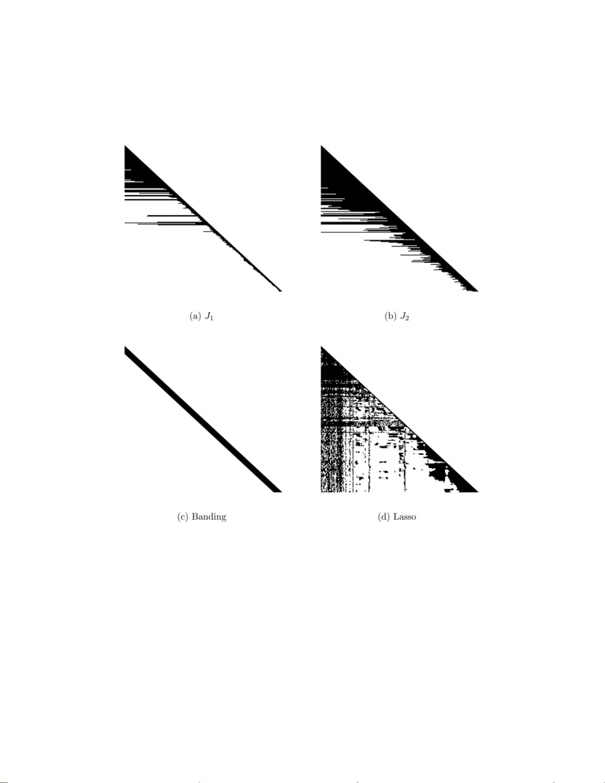
The Annals of Applie d Statistics 2008, V ol. 2, No. 1, 245–26 3 DOI: 10.1214 /07-A OAS139 c  Institute of Mathematical Statistics , 2008 SP ARSE ESTIMA TION OF LAR GE CO V ARIANCE MA TRICES VIA A NESTED LASSO PENAL TY By Eliza vet a Levina, 1 Adam R othman and Ji Zhu 2 University of Michigan The pap er proposes a new co v ariance estimator for large co v ari- ance matrices w hen the v ariables hav e a natural ordering. U sing the Cholesky decomposition of the inv erse, w e imp ose a banded structure on the Cholesky facto r, and select the bandwidth adaptively for each ro w of the Cholesky factor, using a nov el p enalty w e call nested Lasso. This structure has more flexibility than regular banding, but, u nlike regular Lasso applied to the entries of the Cholesky factor, results in a sparse estimator for the inv erse of the co v ariance matrix. An it- erativ e algorithm for solving the optimization problem is d eveloped. The estimator i s compared to a num b er of other cov ariance estima- tors and is shown to do b est, b oth in simulatio ns and on a real data example. Simulations sh ow that the margin by whic h the estimator outp erforms its comp etitors t ends to increase with dimension. 1. Introduction. Estimating co v ariance matrices has alw a ys b een an im- p ortan t p art of m u ltiv ariate an alysis, and estimating large co v ariance ma- trices (where the d imension of the d ata p is comparable to or larger than the sample size n ) has gained p articular atten tion recen tly , since high- dimensional data are so common in mo d ern applicatio ns (gene arrays, fMRI, sp ectroscopic imaging, and man y others). There are many statistical meth- o ds that require an estimate of a cov ariance matrix. They include princi- pal comp onent analysis (PCA), linear and quadr atic d iscriminan t analysis (LD A and QDA ) for classification, regression for m ultiv ariate norm al data, inference ab out fun ctions of the means of the comp onen ts (e.g., ab out the mean resp onse curv e in longitudinal studies), and analysis of ind ep endence and conditional indep enden ce r elatio nships b et w een comp onen ts in graph i- cal mo dels. Note that in man y of these applications (LD A, regression, con- ditional indep end en ce analysis) it is not the p opu lation co v ariance Σ itself Received Marc h 2007; revised S eptember 2007. 1 Supp orted in part by NSF Gran t D MS-05-05424 and NSA Grant MSPF-04Y-120. 2 Supp orted in part by NSF Gran ts DMS- 05-05432 and D MS-07-05532 . Key wor ds and phr ases. Co v ariance matrix, h igh dimension lo w sample size, large p small n , Lasso, sparsit y , Cholesky decomp osition. This is a n electronic repr in t of the o r iginal article published by the Institute of Ma thematical Statistics in The Annals of Applie d Statistics , 2008, V ol. 2, No. 1 , 245–26 3 . This r eprint differs from the origina l in pagination and typogra phic detail. 1 2 E. LEVIN A, A. ROTHMAN AND J. ZH U that needs estimating, but its in v ers e Σ − 1 , also known as the precision or concen tration matrix. When p is s m all, an estimate of one of these matrices can easily b e inv erted to obtain an estimate of the other one; but when p is large, inv ersion is problematic, an d it ma y make more sense to estimate the needed matrix directly . It has long b een kno wn that the sample co v ariance matrix is an extremely noisy estimator of the p opu lation co v ariance matrix when p is large, although it is alwa ys unbia sed [ Dempster ( 1972 )]. There is a fair amount of theoreti- cal work on eigen v alues of sample co v ariance matrices of Gaussian data [see Johnstone ( 200 1 ) for a review] th at sh ows that un less p/n → 0, the eigenv al- ues of the sample co v ariance matrix are more s p read out than the p opu lation eigen v alues, ev en asymptotical ly . Consequen tly , man y alternativ e estimators of the co v ariance ha v e b een p r op osed. Regularizing large co v ariance matrices by Steinian shrink age has b een prop osed early on, and is achiev ed b y either shrinking the eigen v alues of the sample co v ariance matrix [ Haff ( 1980 ); Dey and Sr iniv asan ( 1985 )] or replacing the sample cov ariance w ith its linear com bination with the iden- tit y matrix [ Ledoit and W olf ( 2003 )]. A linear com bination of the samp le co v ariance and the iden tit y matrix has also b een used in some applications— for example, as original motiv ation f or rid ge regression [ Ho erl and Kennard ( 1970 )] and in regularized discrimin ant analysis [ F riedman ( 1989 )]. These approac hes d o not affect the eigen ve ctors of the co v ariance, only the eigen- v alues, and it has b een sho w n that the samp le eigen v ectors are also not consisten t when p is large [ Johnstone and L u ( 200 7 )]. Hence, shrink age esti- mators ma y not do w ell for P C A. I n the conte xt of a factor analysis mo del, F an et al. ( 2008 ) develo p ed high-dimensional estimators for b oth the cov ari- ance and its inv erse. Another general approac h is to regularize the sample co v ariance or its in verse by making it sparse, u sually by setting some of the off-diagonal elemen ts to 0. A n u m b er of metho d s exist that are particularly useful when comp onen ts ha ve a natural ordering, f or example, f or longitudinal d ata, where the n eed for imp osing a structure on th e cov ariance h as long b een recognized [see Diggle and V erbyla ( 1998 ) for a r eview of the longitudinal data literature]. Such stru ctur e often implies that v ariables far apart in this ordering are only weakly correlated. Banding or tap ering the co v ariance matrix in this conte xt h as b een pr op osed by Bic k el and Levina ( 2004 ) and F urrer and Bengtsson ( 2007 ). Bic ke l and Levina ( 2007 ) show ed consistency of banded estimato rs un d er mild conditions as long as (log p ) /n → 0, for b oth band ing the co v ariance matrix and the Cholesky factor of the in v erse discussed b elo w. They also pr op osed a cross-v alidation approac h for selecting the band width. Sparsit y in the inv erse is particularly usefu l in graphical mo dels, since zero es in the inv erse imply a graph structure. Banerjee et al. ( 2006 ) and SP A R SE ESTIMA TION OF LARGE CO V ARI A NCE MA TRICES 3 Y uan and Lin ( 2007 ), usin g differen t semi-defin ite programming algo rithms, b oth ac hiev e sparsit y b y p enalizing the normal lik eliho o d with an L 1 p enalt y imp osed dir ectly on the elemen ts of the in v erse. T h is approac h is compu- tationall y v ery in tensiv e and do es not scale w ell with dimension, but it is in v ariant und er v ariable p ermutati ons. When a natural ordering of the v ariables is a v ailable, sp arsit y in the in- v erse is usually in tro duced via the mo d ified Cholesky decomp osition [ P our ahmadi ( 1999 )], Σ − 1 = T ⊤ D − 1 T . Here T is a low er triangular matrix with ones on the diagonal, D is a di- agonal m atrix, and the elemen ts b elo w diagonal in the i th ro w of T can b e in terp reted as regression co efficien ts of the i th comp onent on its predeces- sors; the element s of D giv e the corresp onding prediction v ariances. Sev eral approac h es to in tro d ucing zeros in the Cholesky factor T ha v e b een pr op osed. While they are not inv ariant to p ermutatio ns of v ariables and are thus most natural wh en v ariables are ordered, they do introduce sh r ink- age, and in some cases, sparsit y , in to the estimator. W u and Pourahmadi ( 2003 ) p rop ose a k -diagonal (band ed) estimator, which is obtained by smo oth- ing along the first k su b-diagonals of T , and sett ing the rest to 0. Th e n um b er k is c h osen via an AIC p enalt y on the normal lik eliho o d of the data. The re- sulting estimate of th e in verse is also k -banded. W u and P ourahmadi ( 200 3 ) sho wed elemen t-wise consistency of their estimator (although that is a p rop- ert y sh ared by the sample co v ariance matrix), and Bic k el and Levina ( 2007 ) sho wed that b anding the Cholesky factor p ro duces a consistent estimator in the matrix L 2 norm under wea k conditions on the co v ariance matrix, the most general theoretical result on band ing a v ailable to date. Huang et al. ( 2006 ) prop osed adding an L 1 p enalt y on the elemen ts of T to the nor- mal lik eliho o d, w hic h leads to Lasso-t yp e shrink age of the co efficien ts in T , and introd uces zeros in T which can b e p laced in arbitrary lo cations. This approac h is m ore flexible than band in g, but th e resu lting estimate of the in verse ma y not h av e any zeros at all, hence, the sparsit y is lost. No con- sistency results are a v ailable for this m etho d . A related Ba yesia n approac h [ Smith and Kohn ( 2002 )] in tro duces zeros in the Cholesky factor via a hier- arc hical pr ior, while W ong et al. ( 2003 ) use a pr ior that allo ws elemen ts of the inv erse itself to b e zero. Our approac h, whic h we will call adaptive b anding in contras t to regular banding, also relies on the Ch olesky decomp osition and a natural ordering of the v ariables. By introducing a no vel nested Lasso p enalt y on the co- efficien ts of r egressions that form the m atrix T , we select the b est mo del that regresses the j th v ariable on its k closest p redecessors, but, u nlik e in simple banding, we allo w k = k j to d ep end on j . Th e resulting structure of 4 E. LEVIN A, A. ROTHMAN AND J. ZH U Fig. 1. The plac ement of zer os in the Cholesky facto r T : (a) Banding; (b) L asso p enalty of Huang et al.; (c) A daptive b anding. the Cholesky f actor is illustrated in Figure 1 (c). It is ob viously more flexible than banding, and hence, sh ould pro duce a b etter estimate of the co v ariance b y b eing b etter able to adap t to the data. Unlik e the Lasso of Huang et al. ( 2006 ), adaptive banding preserves sparsit y in the resulting estimate of the in verse, sin ce the matrix T is still banded, with the o ve rall k = max j k j . W e sho w that adaptiv e band in g, in addition to preserving sparsit y , outp erform s the estimator of Huang et al. ( 2006 ) in s im u lations and on r eal d ata. One ma y also reasonably exp ect that as long as the p enalt y tun ing parameter is selecte d appropriately , the theoretica l consistency r esults established f or banding in Bic k el and Levina ( 2007 ) w ill h old for adaptive band ing as well . The rest of the pap er is organized as follo ws: Section 2 su mmarizes the p enalized estimation app roac h in general, and p resen ts the nested Lasso p enalt y and the adaptiv e b anding algorithm, with a detailed discus sion of optimizatio n issues. Section 3 presen ts numerica l results for adaptiv e band- ing an d a num b er of other metho ds, for simulate d data and a r eal example. Section 4 concludes with d iscussion. 2. Metho ds for p enalized estimation of the C holesky factor. F or the sak e of completeness, w e start from a brief summ ary of the formal deriv ation of the Cholesky decomp osition of Σ − 1 . S upp ose we hav e a rand om ve ctor X = ( X 1 , . . . , X p ) ⊤ , with mean 0 and co v ariance Σ . Let X 1 = ε 1 and, for j > 1, let X j = j − 1 X l =1 φ j l X l + ε j , (1) where φ j l are th e co efficient s of the b est linear predictor of X j from X 1 , . . . , X j − 1 and σ 2 j = V ar( ε j ) the corresp onding residual v ariance. L et Φ b e the lo wer tri- angular matrix with j th row cont aining the co efficient s φ j l , l = 1 , . . . , j − 1, SP A R SE ESTIMA TION OF LARGE CO V ARI A NCE MA TRICES 5 of the j th r egression ( 1 ). Note that Φ has zeros on th e diagonal. Let ε = ( ε 1 , . . . , ε p ) ⊤ , and let D = diag( σ 2 j ) b e a diagonal m atrix with σ 2 j on the diagonal. Rewriting ( 1 ) in matrix form give s ε = ( I − Φ) X , (2) where I is the identit y matrix. It follo ws from standard regression theory that the residuals are uncorrelated, so taking co v ariance of b oth sides of ( 2 ) giv es D = ( I − Φ)Σ( I − Φ) ⊤ . Letting T = I − Φ , we can now wr ite do w n the mo dified Cholesky d ecom- p ositions of Σ and Σ − 1 : Σ = T − 1 D ( T − 1 ) ⊤ , Σ − 1 = T ⊤ D − 1 T . (3) Note that the only assumption on X was mean 0 ; normalit y is n ot requ ir ed to derive the Cholesky d ecomp ositi on. The natur al question is h o w to estimate the m atrices T and D from data. Th e standard r egression estimates can b e compu ted as long as p ≤ n , but in h igh-dimensional situations one exp ects to d o b ett er b y r egularizing the co efficien ts in T in some wa y , for the same reasons one ac hiev es b etter prediction from regularized regression [ Hastie et al. ( 2001 )]. If p > n , the regression p r oblem b ecomes singu lar, and some r egularizati on is necessary for the estimator to b e w ell defined. 2.1. A daptive b anding with a neste d L asso p e nalty. The method s pr o- p osed b y Huang et al. ( 2006 ) and W u and P ourahmadi ( 2003 ) b oth assume the data x i , i = 1 , . . . , n , are samp led from a normal distribution N ( 0 , Σ ) and use the normal lik eliho o d as the loss function. As the deriv ation ab o v e sho w s, the normalit y assump tion is n ot n ecessary for estimating co v ariance using the Cholesky d ecomp osition. W e start, ho w ever, with the normal lik eli- ho o d as the loss fu nction and demons trate ho w a new p enalt y can b e applied to pro d uce an adaptiv ely b anded estimator. The negativ e log-lik eliho o d of the data, up to a constan t, is giv en by ℓ (Σ , x 1 , . . . , x n ) = n log | Σ | + n X i =1 x ⊤ i Σ − 1 x i (4) = n log | D | + n X i =1 x ⊤ i T ⊤ D − 1 T x i . The negativ e log-lik eliho o d can b e decomp osed into ℓ (Σ , x 1 , . . . , x n ) = p X j =1 ℓ j ( σ j , φ j , x 1 , . . . , x n ) , 6 E. LEVIN A, A. ROTHMAN AND J. ZH U where ℓ j ( σ j , φ j , x 1 , . . . , x n ) = n log σ 2 j + n X i =1 1 σ 2 j x ij − j − 1 X l =1 φ j l x il ! 2 . (5) Minimizing ( 4 ) is equiv alen t to minimizing eac h of the fu nctions ℓ j in ( 5 ), whic h is in turn equiv alen t to compu ting the b est least squares fit for eac h of the r egressions ( 1 ). W u and Pourahmadi ( 2003 ) suggested using an AIC or BIC p enalt y to se- lect a common order for the regressions ( 1 ). They also subsequent ly smo oth the sub-diagonals of T , and their metho d’s p erformance d ep ends on the exact c h oice of th e sm o other and the selection of the smo othing parame- ters as m uc h as on the choic e of ord er. This make s a direct comparison to Huang et al. ( 2006 ) and our o wn metho d difficult. Bic k el and Levina ( 2007 ) prop osed a cross-v alidation m etho d for selecting the common ord er for the regressions, and we will u s e their metho d for all the (nonadaptive ) band ing results b elo w. Huang et al. ( 2006 ) p rop osed adding a p enalt y to ( 4 ) and m inimizing ℓ (Σ , x 1 , . . . , x n ) + λ p X j =2 P ( φ j ) , (6) where the p enalt y P on the ent ries of φ j = ( φ j 1 , . . . , φ j,j − 1 ) is P ( φ j ) = k φ j k d d , (7) and k · k d is the L d v ector norm w ith d = 1 or 2. The L 2 p enalt y ( d = 2 ) do es n ot r esu lt in a sp arse estimate of the co v ariance, so w e w ill n ot fo cu s on it here. The L 1 p enalt y ( d = 1 ), that is, the L asso p enalt y [ Tibshirani ( 1996 )], results in zeros irregularly placed in T a s shown in Figure 1 (b), whic h also do es not pr o duce a spars e estimate of Σ − 1 . Again, minimizing ( 6 ) is equiv alen t to separately minimizing ℓ j ( σ j , φ j , x 1 , . . . , x n ) + λP ( φ j ) , (8) with P ( φ 1 ) = 0. W e prop ose replacing the L 1 p enalt y λ P j − 1 l =1 | φ j l | with a new ne ste d Lasso p enalt y , J 0 ( φ j ) = λ  | φ j,j − 1 | + | φ j,j − 2 | | φ j,j − 1 | + | φ j,j − 3 | | φ j,j − 2 | + · · · + | φ j, 1 | | φ j, 2 |  , (9) where we define 0 / 0 = 0 . Th e effect of this p enalt y is that if the l th v ariable is not included in the j th regression ( φ j l = 0), then all the s u bsequent v ariables ( l − 1 through 1) are also excluded, since giving them nonzero co efficien ts w ould result in an infinite p enalt y . Hence, the j th r egression only uses k j ≤ SP A R SE ESTIMA TION OF LARGE CO V ARI A NCE MA TRICES 7 j − 1 closest predecessors of the j th co ordinate, and eac h regression h as a differen t order k j . The scaling of coefficients in ( 9 ) could b e an issu e: the sole co efficient φ j,j − 1 and the r atios | φ j,t | | φ j,t +1 | can, in prin ciple, b e on differen t scales, and p enalizing them with the same tuning p arameter λ ma y not b e appropriate. In s ituations where the data ha v e natural ordering, the v ariables are often measuremen ts of the same quantit y o ve r time (or o ver some other index, e.g., spatial lo cation or sp ectral w a vele ngth), so b oth the individual co efficien ts φ j,t and their ratios are on the order of 1; if v ariables are rescaled, in th is con text they w ould all b e rescale d at the same time (e.g., con v erting b et w een differen t units). Ho wev er, the nested L asso p enalt y is of indep endent inte rest and ma y b e used in other con texts, f or example, for group v ariable selec tion. T o address the scaling issu e in general, we prop ose t wo easy mo d ifi cations of the p enalt y ( 9 ): J 1 ( φ j ) = λ  | φ j,j − 1 | | ˆ φ ∗ j,j − 1 | + | φ j,j − 2 | | φ j,j − 1 | + | φ j,j − 3 | | φ j,j − 2 | + · · · + | φ j, 1 | | φ j, 2 |  , (10) J 2 ( φ j ) = λ 1 j − 1 X t =1 | φ j,t | + λ 2 j − 2 X t =1 | φ j,t | | φ j,t +1 | , (11) where ˆ φ ∗ j,j − 1 is the coefficient from regressing X j on X j − 1 alone . The ad- v an tage of the first p enalt y , J 1 , is that it still requires only one tuning parameter λ ; the disadv an tage is th e ad ho c use of the regression co efficient ˆ φ ∗ j,j − 1 , whic h m ay not b e close to ˆ φ j,j − 1 , but w e can reasonably hop e is on the same scale. T he second p enalt y , J 2 , do es n ot require this extra regres- sion co efficient, bu t it d o es r equire selection of t wo tuning parameters. It turns out, h o wev er, that, in p ractice, the v alue of λ 2 is not as imp ortan t as that of λ 1 , as the ratio term will b e infinite wheneve r a coefficient in th e denominator is sh runk to 0. In pr actice, on b oth simulat ions and real data, w e hav e n ot found m uc h difference b et w een the three versions J 0 , J 1 , and J 2 , although in general J 1 tends to b e b etter than J 0 , and J 2 b etter than J 1 . In wh at follo w s, we will write J for the three nested p enaltie s J 0 , J 1 and J 2 if any one of them can b e su bstituted. Adaptiv e banding for co v ariance estimation: 1. F or j = 1, ˆ σ 2 1 = V ar ( X 1 ). 2. F or eac h j = 2 , . . . , p , let ( ˆ σ j , ˆ φ j ) = arg min σ j ,φ j ℓ j ( σ j , φ j , x 1 , . . . , x n ) + J ( φ j ) . (12) 3. Compu te ˆ Σ − 1 according to ( 3 ); let ˆ Σ = ( ˆ Σ − 1 ) − 1 . 8 E. LEVIN A, A. ROTHMAN AND J. ZH U 2.2. The algorith m. Th e minimization of ( 12 ) is a non trivial problem, since the p enaltie s J are not conv ex. W e dev elop ed an iterativ e pro cedur e for this minimization, wh ic h we foun d to w ork w ell and con v erge quic kly in practice. The algorithm requires an initial estimate of the co efficien ts φ j . In the case p < n , one could initialize w ith co efficien ts ˆ φ j fitted without a p enalt y , whic h are giv en by the usual least squares estimates from regressing X j on X j − 1 , . . . , X 1 . If p > n , ho w ev er, these are not d efined. Instead, we in i- tialize with ˆ φ (0) j t = ˆ φ ∗ j t , wh ich are found by r egressing X j on X t alone, for t = 1 , . . . , j − 1. Then w e iterate b et w een steps 1 and 2 until con verge nce. Step 1. Giv en ˆ φ ( k ) j , solv e for ˆ σ ( k ) j (the r esidual sum of squares is giv en in closed form ): ( ˆ σ ( k ) j ) 2 = 1 n n X i =1 x ij − j − 1 X t =1 ˆ φ ( k ) j t x it ! 2 . Step 2. Giv en ˆ φ ( k ) j and ˆ σ ( k ) j , solv e for ˆ φ ( k +1) j . Here we u se th e follo win g standard lo cal quadratic approximat ion [also used b y F an and L i ( 2001 ) and Huang et al. ( 2006 ), among others]: | φ ( k +1) j t | ≈ ( φ ( k +1) j t ) 2 2 | φ ( k ) j t | + | φ ( k ) j t | 2 . (13) This appro ximation, together with substituting the p revious v alues φ ( k ) j t in the denominator of the ratios in the p enalt y , con verts the minimization int o a ridge (quadratic) p roblem, which can b e s olv ed in closed f orm. F or example, for the J 2 p enalt y , we s olv e ˆ φ ( k +1) j = arg min φ j 1 ( ˆ σ ( k ) j ) 2 n X i =1 x ij − j − 1 X t =1 φ j t x it ! 2 + λ 1 j − 1 X t =1 φ 2 j t 2 | ˆ φ ( k ) j t | + λ 2 j − 2 X t =1 φ 2 j t 2 | ˆ φ ( k ) j t | · | ˆ φ ( k ) j,t +1 | . F or numerical stabilit y , we threshold the abs olute v alue of eve ry estimate at 10 − 10 o ver different iterations, and at the end of the iterations, set all estimates equal to 10 − 10 to zero. The app ro ximation for J 0 and J 1 p enalties is analogous. The function we are min imizing in ( 12 ) is not con vex, there- fore, there is n o guaran tee of findin g the global m in im u m. Ho wev er, in the sim u lations we ha v e tried, w here we kno w the un derlying truth (see Section 3.1 for details), w e ha v e not encount ered any problems with spurious local minima with the c h oice of starting v alues describ ed ab ov e. SP A R SE ESTIMA TION OF LARGE CO V ARI A NCE MA TRICES 9 Another approac h in Step 2 ab ov e is to use the “sho oting” s trategy [ F u ( 1998 ); F riedm an et al. ( 2007 )]. That is, we sequentia lly solve for φ j t : for eac h t = 1 , . . . , j − 1, we fix σ j and φ − j t = ( φ j 1 , . . . , φ j,t − 1 , φ j,t +1 , . . . , φ j,j − 1 ) ⊤ at their most recent estimates and minimize ( 12 ) o ver φ j t , and iterate until con verge nce. Since eac h minimization o v er φ j t in volv es only one parameter and the ob jectiv e fu nction is p iecewise conv ex, the computation is trivial. Also, since at eac h iteration the v alue of th e ob jectiv e fun ction decreases, con verge nce is guarantee d. In our exp erience, these t wo ap p roac hes, the lo cal quadratic approximat ion and the sh o oting strategy , do not differ m u c h in terms of th e computational cost and the solutions they offer. The algorithm also requires selecting the tuning p arameter λ , or, in the case of J 2 , tw o tu n ing parameters λ 1 and λ 2 . W e selected tuning p arameters on a v alidation set whic h we set aside from the original training data; alter- nativ ely , 5-fold cross-v alidation can b e u sed. As discussed ab o v e, we found that the v alue of λ 2 in J 2 is not as imp ortan t; ho wev er, in all examples in this pap er the computational burd en wa s small enough to optimize o ver b oth parameters. 3. Numerical results. In this section we compare adaptiv e banding to other metho ds of regularizing the inv erse. Our primary comparison is w ith the Lasso m etho d of Huang et al. ( 2006 ) and with nonadaptiv e banding of Bic k el and Levina ( 200 7 ); these metho ds are closest to ours and also pro vide a sp arse estimate of the Cholesky factor. As a b enchmark, w e also include the shrink age estimator of Ledoit and W olf ( 2003 ), whic h do es not dep end on the ord er of v ariables. 3.1. Simulation data. Sim ulations we re carried out for three different co v ariance m o dels. The first one h as a tri-diagonal Ch olesky factor and , hence, a tri-diagonal inv erse: Σ 1 : φ j,j − 1 = 0 . 8; φ j,j ′ = 0 , j ′ < j − 1; σ 2 j = 0 . 01 . The second one has entries of the Cholesky factor exp onen tially deca ying as one mo ves a wa y from the diagonal. Its in v erse is not sparse, b ut instead has many small en tries: Σ 2 : φ j,j ′ = 0 . 5 | j − j ′ | , j ′ < j ; σ 2 j = 0 . 01 . Both these mo dels were considered by Huang et al. ( 2006 ), and similar mo dels w ere also considered by Bic k el and Levina ( 2007 ). In b oth Σ 1 and Σ 2 , all the ro ws ha ve the same structure, w hic h fav ors regular nonadaptiv e banding. 10 E. LEVIN A, A. ROTHMAN AND J. ZH U T o test the abilit y of our algorithm to adapt, w e also considered the follo wing structure: Σ 3 : k j ∼ U (1 , ⌈ j / 2 ⌉ ); φ j,j ′ = 0 . 5 , k j ≤ j ′ ≤ j − 1; φ j,j ′ = 0 , j ′ < k j ; σ 2 j = 0 . 01 . Here U ( k 1 , k 2 ) denotes an integ er selected at random from all in tegers from k 1 to k 2 . F or mo d erate v alues of p , this stru cture is stable, and this is w hat w e generate for p = 30 in the simulatio ns b elo w. F or larger p , some realizations can generate a p oorly conditioned true co v ariance matrix, wh ic h is n ot a problem in principle, b ut mak es computing p erformance measures a wkw ard. T o av oid this p r oblem, we divided the v ariables for p = 100 and p = 200 into 3 and 6 indep endent blo c ks, resp ectiv ely , and generate d a random structure from the mo del describ ed ab o v e for eac h of the b lo c ks. W e will r efer to all these mo dels as Σ 3 . The stru cture of Σ 3 should b enefit more f rom adaptiv e banding. F or eac h of the co v ariance mo dels, w e generated n = 100 training observ a- tions, along w ith a separate set of 100 v alidation observ ations. W e considered three different v alues of p : 30 , 100 and 200, and t wo differen t distributions: normal and multiv ariate t w ith 3 degrees of freedom, to test the b eha v- ior of the estimator on hea vy-tailed data. The estimators w ere computed on the training data, with tuning parameters for all metho ds selected b y maximizing the lik eliho o d on the v alidation data. Using these v alues of the tuning parameters, w e then compu ted the estimated co v ariance matrix on the training data and compared it to the true co v ariance matrix. There are m an y criteria one can u se to ev aluate co v ariance matrix esti- mation, for example, any one of the matrix n orms can b e calculated for the difference ( L 1 , L 2 , L ∞ , or F r ob enius n orm). Th ere is n o general agreemen t on which loss to us e in whic h situation. Here we us e the Kullbac k–Leibler loss f or the concen tration matrix, whic h was used in Y uan and Lin ( 2007 ). The Kullback– Leibler loss is d efined as follo ws: ∆ KL ( Σ , ˆ Σ ) = tr( ˆ Σ − 1 Σ ) − ln | ˆ Σ − 1 Σ | − p. (14) Another p opular loss is the entro p y loss for the co v ariance matrix, whic h was used b y Huang et al. ( 2006 ). T h e en tropy loss is the same as the Kullbac k– Leibler loss except the roles of the co v ariance m atrix and its inv erse are switc hed. The entrop y loss can b e derived from the Wishart likel iho o d [ Anderson ( 1958 )]. While one do es not expect ma jor disagree men ts b et w een th ese losses, the en trop y loss is a more appr opriate measure if the co v ariance matrix itself is the primary ob ject of int erest (as in PC A, e.g.), and the Kullbac k–Leibler loss is a more d irect measure of the estimate of th e con- cen tration matrix. Both these losses are not normalized by dimens ion and SP A R SE ESTIMA TION OF LARGE CO V ARI A NCE MA TRICES 11 therefore cannot b e compared dir ectly for different p ’s. W e ha ve also tried matrix norms and the so-calle d quadratic loss f r om Huang et al. ( 2006 ) and found that, while there is no p erfect agreemen t b et we en results ev ery time, qualitativ ely they are quite similar. T he main conclusions we dra w from comparing estimators usin g the Kullbac k–Leibler loss w ould b e the same if an y other loss had b een used. The results for th e normal d ata and the three mo d els are sum marized in T able 1 , whic h giv es the a verag e losses and the corresp onding standard errors ov er 50 replications. T he NA v alues for the sample app ear when the matrix is singular. The J 0 p enalt y has b een omitted b eca use it is dominated b y J 1 and J 2 . In general, w e see that banding and adaptiv e bandin g p erform b ett er on all three mo d els than the sample, Ledoit–W olf ’s estimato r and Lasso. On Σ 1 and Σ 2 , as exp ected, b anding and adaptive band in g are v ery similar (par- ticularly once standard errors are take n in to acco unt) ; but on Σ 3 , adaptiv e banding do es b etter, and the larger p , the bigger the difference. Also, f or normal data th e J 2 p enalt y alw a ys d ominates J 1 , though they are qu ite close. T o test the b eha vior of the metho ds with h eavy- tailed d ata, w e also p er- formed simulati ons for the same three co v ariance mo dels u nder the multi- v ariate t 3 distribution (the hea viest-tail t distribution with fi nite v ariance). T able 1 Multivariate normal simulations for mo dels Σ 1 (b ande d Cholesky f actor), Σ 2 (nonsp arse Cholesky factor with elements de c aying exp onential ly as one moves away fr om the diagonal) and Σ 3 (sp arse Cholesky f actor with variable length r ows). The Kul l b ack–L eibler losses (me ans and, i n p ar entheses, standar d err ors for the me ans over 50 r eplic ations) ar e r ep orte d f or sample c ovarianc e, the shrinkage estimator of L e doit and Wolf ( 2003 ), the L asso metho d of Huang et al. ( 2006 ), the nonadaptive b anding metho d of Bickel and L evina ( 2007 ), and our adaptive b anding wi th p enalties J 1 and J 2 p Sample Ledoit–W olf Lasso J 1 J 2 Banding Σ 1 30 8.3 8(0.14) 3.59(0.04 ) 1 . 26(0 . 04) 0 . 79(0 . 02) 0 . 64(0 . 02) 0 . 63(0 . 0 2) 100 NA 29.33(0 .12) 6 . 91(0 . 11) 2 . 68(0 . 04) 2 . 21(0 . 03) 2 . 21(0 . 03) 200 NA 90.86(0 .19) 14 . 57(0 . 13 ) 5 . 10(0 . 06 ) 4 . 35(0 . 05 ) 4 . 34(0 . 05 ) Σ 2 30 8.3 8(0.14) 3.59(0.02 ) 2 . 81(0 . 04) 1 . 42(0 . 03) 1 . 32(0 . 02) 1 . 29(0 . 0 3) 100 NA 18.16(0 .02) 16 . 12(0 . 09 ) 5 . 01(0 . 07 ) 4 . 68(0 . 06 ) 4 . 55(0 . 05 ) 200 NA 40.34(0 .02) 32 . 84(0 . 11 ) 9 . 88(0 . 06 ) 9 . 28(0 . 06 ) 8 . 95(0 . 06 ) Σ 3 30 8.6 8(0.12) 171. 31(1.00) 4 . 62(0 . 07) 3 . 2 6(0 . 05) 3 . 1 4(0 . 06) 3 . 82(0 . 05) 100 NA 945.65 (2.15) 35 . 60(0 . 7 1) 11 . 82(0 . 13 ) 11 . 24(0 . 12) 14 . 34 (0 . 09) 200 NA 193 8.32(3.0 4) 11 8 . 84(1 . 54) 23 . 3 0(0 . 17) 22 . 70(0 . 16) 29 . 50(0 . 14) 12 E. LEVIN A, A. ROTHMAN AND J. ZH U These resu lts are giv en in T able 2 . All metho ds p erform worse than they do for normal data, but band ing and adaptiv e banding still do b ette r than other metho ds. Because the standard errors are larger, it is hard er to establish a uniform winner among J 1 , J 2 and b anding, but generally these results are consisten t with results obtained for normal data. Finally , w e n ote that the differences b et w een estimators are amplified with gro wing dimen s ion p : while the patterns remain the same for all three v alues of p considered (30, 100 and 200), quant itativ ely the improv emen t of adaptiv e banding o ver the Ledoit–W olf estimator and Lasso is the largest at p = 200, and is exp ected to b e ev en more f or higher dimens ions. Since one adv an tage of adaptiv e b anding as compared to Lasso is p re- serving sparsit y in the in v erse itself, w e also compared p ercent ages of true zeros b oth in the Cholesky factor and in the inv erse that were estimated as zeros, for the mo d els Σ 1 and Σ 3 ( Σ 2 is not sp arse). The r esults are sho wn in T able 3 . While for the easier case of Σ 1 all metho ds do a reasonable job of finding zeros in the Cholesky facto r, Lasso loses them in the in verse, whereas b oth kin d s of banding do not. T his effect is even more apparen t on the more c hallenging case of Σ 3 . T o gain add itional insight in to the sp arsit y of structures pro duced by the differen t metho ds, we also sho w heatmap plots of the p ercen tage of times eac h en try of the Cholesky factor (Figure 2 ) and th e inv erse itself (Figure 3 ) w ere estimated as zeros. It is clear that only adaptive band ing reflects the true und erlying structure. Ov erall, the simula tions show that th e adaptiv e b anding ac hieve s the goals that it was designed for: it h as m ore flexibilit y than banding, and therefore is b etter able to capture the und erlying sparse structure, but, u nlik e the T able 2 Multivariate t 3 simulations for mo dels Σ 1 , Σ 2 , Σ 3 . Descriptions for the entries ar e the same as those in T able 1 p Sample L edoit–W olf Lasso J 1 J 2 Banding Σ 1 30 30.33(0 .65) 9 . 22(0 . 65) 7 . 60(0 . 74) 4 . 32(0 . 21) 3.6 8(0.19) 4.22(0. 60) 100 NA 58 . 24(2 . 61) 38 . 99(1 . 44) 15 . 58(0 . 78 ) 13.85(0 .72) 13.74(0 .72) 200 NA 139 . 21(3 . 0 2) 111 . 62(2 . 73 ) 31 . 45(1 . 80) 28 .22(1.71 ) 27.95(1.70 ) Σ 2 30 30.33(0 .65) 6 . 20(0 . 15) 8 . 44(0 . 20) 5 . 91(0 . 24) 5.2 1(0.22) 5.23(0. 24) 100 NA 24 . 37(0 . 67) 31 . 92(0 . 83) 21 . 76(0 . 76 ) 18.87(0 .71) 19.33(0 .85) 200 NA 50 . 40(1 . 41) 64 . 28(1 . 98) 44 . 58(2 . 00 ) 38.46(1 .75) 39.81(1 .98) Σ 3 30 30.77(0 .74) 199 . 73(4 . 32) 14 . 48(0 . 40) 11 . 47(0 . 4 4) 11.57(0 .47) 11.69(0 .39) 100 NA 1061 . 54(12 . 62) 82 . 05(1 . 4 7) 43 . 38(1 . 14) 4 5.01(1.1 3) 42.78(1.0 4) 200 NA 2182 . 54(21 . 29) 182 . 82(9 . 51) 87 . 5(2 . 75) 9 1.25(2.7 9) 85.65(2.4 9) SP A R SE ESTIMA TION OF LARGE CO V ARI A NCE MA TRICES 13 T able 3 Per c entage of true zer os in the Cholesky factor and in the inverse estimate d as zer os for multivariate normal data, for mo dels Σ 1 and Σ 3 (me ans and, in p ar entheses, standar d err ors for the me ans over 50 r eplic ations) Zeros in the Cholesky factor (%) Zeros in Σ − 1 (%) p Lasso J 1 J 2 Banding Las so J 1 J 2 Banding Σ 1 30 70 . 5(0 . 4) 9 4 . 5(0 . 3 ) 96 . 3(0 . 4 ) 100(0) 3 1.4(0.8) 94.5(0.3) 96.3(0. 4) 100(0) 100 92 . 7(0 . 1) 98 . 6(0 . 04) 99 . 1(0 . 1 ) 100(0) 76.4(0.5) 98.6(0.3) 99.1(0.0 4) 100(0) 200 93 . 7(0 . 06) 99 . 3(0 . 01 ) 99 . 5(0 . 04) 100(0) 69.9(0.4) 99.3(0.0 1) 99.5(0.04) 100(0) Σ 3 30 55 . 6(1 . 5) 8 3 . 2(0 . 5 ) 80 . 9(0 . 7 ) 72.1(0. 9) 10.2(0. 7) 75.3(0.9) 70.4(1.5) 73.1(0.7) 100 88 . 3(0 . 1) 94 . 9(0 . 1) 9 4 . 9(0 . 1) 9 2.8(0.2 ) 55.1(0.5) 92.3(0.3) 92.3(0.2) 93.5(0.2) 200 92 . 4(0 . 1) 97 . 6(0 . 04) 97 . 7(0 . 0 4) 96.7(0.1) 84.4(0.9) 96.6(0.1) 96.7(0.1 ) 97.1(0. 1) Fig. 2. He atmap plots of p er c entage of zer os at e ach l o c ation in the inverse (out of 50 r eplic ations) f or Σ 3 , p = 30 . Bl ack r epr esents 100%, white 0%. Lasso, it h as the abilit y to p reserv e the sparsity in the inv erse as well as in the Ch olesky factor. 14 E. LEVIN A, A. ROTHMAN AND J. ZH U Fig. 3. He atmap plots of p er c entage of zer os at e ach l o c ation in the inverse (out of 50 r eplic ations) f or Σ 3 , p = 30 . Bl ack r epr esents 100%, white 0%. 3.2. Pr ostate c anc e r data. In th is section w e consider an application to a prostate cancer dataset [ Adam et al. ( 2002 )]. T he current standard screening approac h for prostate cancer is a serum test for a p rostate-specific anti gen. Ho wev er, the accuracy is far from satisfactory [ P ann ek and P artin ( 1998 ) and Dja v an et al. ( 1999 )], and it is b eliev ed that a com bination or a p anel of biomarke rs will b e r equired to impr o ve the d etection of prostate can- cer [ Stamey et al. ( 2002 )]. Recent adv ances in h igh-throughput mass sp ec- troscop y ha v e allo wed one to sim ultaneously resolv e and analyze thousands of proteins. In protein mass sp ectrosco p y , we observe , for eac h blo o d seru m sample i , the int ensit y x ij for many time-of-fligh t v alues. Time of flight is related to the mass o ver c h arge ratio m/z of the constituen t pr oteins in the blo o d. The full dataset we consider [ Adam et al. ( 2002 )] consists of 157 health y patien ts and 167 with pr ostate cancer. Th e goal is to discriminate b et w een the tw o groups. F ollo wing the original researc hers, w e ignored m/z - sites b elo w 2000 , where c hemical artifacts can o ccur. T o smo oth the in tensit y profile, w e a vera ge the d ata in consecutiv e blo cks of 10, giving a total of 218 sites. Thus, eac h obs erv ation x = ( x 1 , . . . , x 218 ) consists of an in tensit y p r o- file of length 218, with a kno wn class (cancer or noncancer) mem b ership. The pr ostate cancer dataset we consider comes with pr e-sp ecified training SP A R SE ESTIMA TION OF LARGE CO V ARI A NCE MA TRICES 15 ( n = 216) and test sets ( N = 108). Figure 4 displa ys the mean in tensities for “cancer” and “n oncancer” from the training d ata. W e consider the linear discriminan t metho d (LD A) and the qu adratic discriminan t metho d (QD A). The linear and qu ad r atic d iscriminan t analysis assume the class-conditional d en s it y of x in class k is normal N ( µ k , Σ k ). The LD A arises in the sp ecial case when one assum es that the classes ha ve a common co v ariance matrix Σ k = Σ , ∀ k . If the Σ k are not assumed to b e equal, w e then get Q DA. The linear and quadratic d iscriminan t scores are as follo w s: LD A : δ k ( x ) = x ⊤ ˆ Σ − 1 ˆ µ k − 1 2 ˆ µ ⊤ k ˆ Σ − 1 ˆ µ k + log ˆ π k , QD A : δ k ( x ) = − 1 2 log | ˆ Σ k | − 1 2 ( x − ˆ µ k ) ⊤ ˆ Σ − 1 k ( x − ˆ µ k ) + log ˆ π k , where ˆ π k = n k /n is the pr op ortion of the num b er of class- k observ ations in the training data, and the classification rule is giv en by arg max k δ k ( x ). Detail ed information on LDA and QDA can b e found in Mardia et al. ( 1979 ). Using the training data, we estimate ˆ µ k = 1 n k X i ∈ class k x i and estimate ˆ Σ − 1 or ˆ Σ − 1 k using five different metho d s: the shrink age to ward the iden tit y estimator of Ledoit and W olf ( 2003 ), band ing the C h olesky fac- tor, the Lasso estimator, and our adaptiv e banding metho d; w e also include the Naiv e Ba y es metho d as a b enc hmark, s ince it corresp onds to LD A w ith the co v ariance m atrix estimated by a diagonal matrix. T uning parameters in different metho d s are c hosen via fiv e-fold cross-v alidation based on the training data. Mean vect ors and co v ariance matrices were estimated on the training data and p lugged into the classification rule, whic h w as then ap- plied to the test data. Note that for this d ataset p is greater than n , hence, Fig. 4. The me an intensity for “ c anc er ” and “ nonc anc er ” fr om the tr aining data. 16 E. LEVIN A, A. ROTHMAN AND J. ZH U the sample co v ariance matrix is not inv ertible and cannot b e used in LD A or QDA. The results as measur ed by the test set classificatio n error are su mma- rized in T ab le 4 . F or this particular dataset, w e can see that o v erall the QD A p erforms muc h worse than the LD A, so we fo cus on the results of the L DA. The Naiv e Ba y es metho d , whic h assumes indep endence among v ariables, has the wo rst p erformance. Banding (with a common bandwid th) and the Lasso metho d p erform similarly and b etter than the Naiv e Ba y es metho d . Our adaptiv e banding metho d p erf orms the b est, with either the J 1 or the J 2 p enalt y . T o gain more insigh t ab out the sparsit y stru ctures of differen t estimators, w e p lot the stru ctures of the estimated Cholesky factors and the corresp onding ˆ Σ − 1 of d ifferen t metho d s in Figures 5 and 6 (blac k represents nonzero, and wh ite represents zero). Based on the differences in the clas- sification p erformance, these plots imply that the Lasso metho d may hav e included man y unimp ortan t elemen ts in ˆ Σ − 1 (estimating zeros as nonze- ros), while the band ing metho d ma y h a ve missed some imp ortan t elemen ts (estimating nonzeros as zeros). T he estimate d C h olesky factors and the cor- resp ondin g ˆ Σ − 1 ’s from the adaptiv e b anding metho d ( J 1 and J 2 ) repr esent an in teresting structure: the in tensities at higher m/z -v alues are more or less conditionally indep end ent, while the in tensities at lo we r m/z -v alues show a “blo c k-diagonal” stru cture. W e note that in the abov e analysis we used likel iho o d on the cross- v alidatio n data as the criterion for selecting tun ing p arameters. As an al- ternativ e, w e also considered using the classification error as the selectio n criterion. T he results from the t w o selectio n criteria are similar. F or simplic- it y of exp osition, w e only pr esen ted r esults from using the like liho o d as the selectio n criterion. Finally , we n ote that Adam et al. ( 2002 ) rep orted an error rate around 5% for a four-class ve rsion of this problem, u sing a p eak fin ding pr o ce- dure follo w ed by a decision tree algorithm. Ho w ev er, w e hav e had d iffi- cult y replicating their r esu lts, ev en when using their extracted p eaks. In Tibshirani et al. ( 2005 ) the follo wing classification errors w ere rep orted f or other metho ds applied to the t w o-class dataset we used here: 30 for Nearest Shrun k en Cen troids [ Tibshirani et al. ( 2003 )], and 16 for b oth L asso and fused Lasso [ Tibshirani et al. ( 2005 )]. Ho wev er, note that these authors did not apply blo c k smo othing. T able 4 T est err ors (out of 108 samples) on the pr ostate c anc er dataset Metho d Naive Ba yes Ledoit & W olf Bandi ng Lasso J 1 J 2 T est error (LDA) 32 16 16 18 11 12 T est error (QDA) 32 51 46 49 31 29 SP A R SE ESTIMA TION OF LARGE CO V ARI A NCE MA TRICES 17 Fig. 5. Structur e of Cholesky factors estimate d for the pr ostate data. White c orr esp onds to zer o, black to nonzer o. 4. Su mmary and discuss ion. W e hav e p resen ted a new co v ariance esti- mator for ord ered v ariables with a band ed structure, whic h, by selecting the bandwidth adaptiv ely for eac h r o w of the Cholesky factor, ac hieve s more flexibilit y than regular b anding b ut still p reserv es s parsit y in the inv erse. Adaptiv e banding is ac h iev ed using a no v el nested Lasso p en alt y , whic h tak es into accoun t the ordering structure among th e v ariables. The estima- tor has b een sho w n to do we ll b oth in simulati ons and a real data exam- ple. Zhao et al. ( 2006 ) prop osed a r elated p enalt y , the comp osite absolute p enalt y (CAP), for hand ling hierarc h ical structures in v ariables. Ho wev er, 18 E. LEVIN A, A. ROTHMAN AND J. ZH U Fig. 6. Structur e of the inve rse c ovarianc e matrix estimate d for the pr ostate data. White c orr esp onds to zer o, black to nonzer o. Zhao et al. ( 2006 ) only considered a h ierarch y with t wo leve ls, while, in our setting, there are essentia lly p − 1 hierarc hical lev els; hence, it is not clear ho w to directly apply CAP without dramatically increasing the num b er of tuning parameters. The theoretica l prop erties of the estimator are a sub ject f or fu ture w ork. The nested Lasso p enalt y is n ot conv ex in the parameters; it is like ly that the theory devel op ed b y F an and Li ( 2001 ) for nonconv ex p enalized m axi- m u m lik eliho o d estimation can b e extended to co ver the nested Lasso (it is not directly applicable since our p enalt y cannot b e decomp osed into a su m SP A R SE ESTIMA TION OF LARGE CO V ARI A NCE MA TRICES 19 of identic al p enalties on the ind ividual co efficient s). Ho wev er, that theory w as devel op ed only for the case of fixed p , n → ∞ , and the more r elev ant analysis for estimation of large co v ariance matrices w ould b e und er the as- sumption p → ∞ , n → ∞ , with p growing at a rate equal to or p ossibly faster than that of n , as was done for the b anded estimator by Bic k el and Levina ( 2007 ). Another in teresting q u estion for f u ture work is extending this idea to estimators inv ariable under v ariable p erm u tations. Ac kn o wledgment s. W e thank the Editor, Mic hael Stein, and tw o referees for their feedbac k whic h led us to improv e the pap er, particularly the d ata section. W e also thank Jianqing F an, Xiaoli Meng an d Bin Y u for helpful commen ts. REFERENCES Adam, B., Qu, Y ., Da vis, J., W ard, M., Clements, M. , C azares, L. , Sem mes, O., Schellhammer, P., Y asui, Y., Feng, Z. and Wright, G. (2002). Serum protein fingerprinting coupled with a pattern-matc hing algorithm distinguishes prostate cancer from b enign prostate hyp erplasia and health y men. Canc er R ese ar ch 62 3609–3614. Anderson, T. W. (1958). An Intr o duction to Multivariate Statistic al Analysis . Wiley , New Y ork. MR009158 8 Banerjee, O., d’ Aspremont, A. and El Ghao ui, L. (2006). Sparse cov ariance selection via robust maximum lik elihoo d estimation. In Pr o c e e dings of IC ML . Bickel, P. J. and Levi na, E. (2004 ). Some theory for Fisher’s linear discriminan t func- tion, “naiv e Ba yes,” and some alternatives when there are man y more v ariables th an observ ations. Bernoul li 10 989–1010. MR210804 0 Bickel, P. J. and Levina, E. (2007). Regularized estimation of large cov ariance matrices. An n. Statist. T o app ear. Dempster, A. (1 972). Cov ariance selection. Biometrics 28 157–175. Dey, D. K. and Srini v asan, C. (1985). Estimation of a cov ariance matrix u nder Stein’s loss. Ann. Statist. 13 158 1–1591 . MR08115 11 Diggle, P. and Verbyla, A . (199 8). Nonparametric estimation of cov ariance structure in longitudinal data. Biometrics 54 401–41 5. Dja v a n, B., Zlott a, A., Kra tzik, C., Remzi, M., Seitz, C., Sch ulman, C. and Marberger, M. (1999). Psa , psa density , p sa density of transitio n zone, free/total psa ratio, and psa velocity for early detection of prostate cancer in men with serum psa 2.5 to 4.0 ng/ml. Ur olo gy 54 517–52 2. F an, J., F an, Y. and L v, J. (2008). H igh d imensional cov ariance matrix estimation using a factor mo del. J. Ec onometrics. T o app ear. F an, J. and Li, R. (2001). V ariable selection via nonconca ve p enalized likelihoo d and its oracle prop erties. J. Amer. Stat ist. Asso c. 96 1348–136 0. MR194658 1 Friedman, J. (1989). Regularized discrimi nant analysis. J. Amer. Statist. Asso c. 84 165 – 175. MR099967 5 Friedman, J., Hastie, T., H ¨ ofling, H. G. and Tibshirani , R. (2007). P athw ise co or- dinate optimization. Ann. Appl. St atist. 1 302–3 32. Fu, W. (1998). Penal ized regressions: The bridge vers us the lasso. J. Comput. Gr aph. Statist. 7 397 –416. MR164671 0 20 E. LEVIN A, A. ROTHMAN AND J. ZH U Furrer, R . and Be ngtsson, T. (2007). Estimation of h igh-dimensional prior and p os- terior cov ariance matrices in Kalman filter v ariants. J. Multivariate Anal. 98 227–2 55. MR230175 1 Haff, L. R. (1980). Empirical Bay es estimation of the multiv ariate n ormal cov ariance matrix. Ann. Statist. 8 586–597. MR056872 2 Hastie, T., Ti bshirani, R. and Frie dman, J. (2001). The Elements of Statistic al L e arn- ing . Sp ringer, Berlin. MR1851606 Hoerl, A. E. and Kennard, R. W. (1970). Ridge regression: Biased estimation for nonorthogonal problems. T e chnometrics 12 55–67. Huang, J., Liu, N., Pourahmadi, M. and Li u, L. (2006). Cov ariance matrix selection and estimation via p en alised normal lik elihoo d. Biometrika 93 85–98. MR227774 2 Johnstone, I. M. (2001). On the distribution of the largest eigen v alue in principal com- p onents analysis. Ann. Statist . 29 295–327 . MR186396 1 Johnstone, I. M . and Lu, A. Y. (2007). Sparse principal comp onents analysis. J. A mer. Statist. Asso c. T o app ear. Ledoit, O. and Wo lf, M . (2003). A w ell-conditioned estimator for large-dimensional co v ariance matrices. J. Mul tivariate A nal. 88 365–411. MR202633 9 Mardia, K. V., Kent, J. T. and Bibby, J. M. (1979). Multivariate A nalysis . Academic Press, New Y ork. MR0560319 P annek, J. and P ar tin, A. (1998). The role of psa and p ercent free psa for staging and prognosis pred iction in clinically localized prostate cancer. Semi n. Ur ol. Onc ol. 16 100–10 5. Pourahmadi, M. (1999 ). Join t mean-cov ariance mo dels with applications to longitudinal data: Unconstrained parameterisation. Biometrika 86 677–69 0. MR172378 6 Smith, M. and Kohn, R. (2002 ). Pars imonious co v ariance matrix estimation for longitu- dinal data. J. Amer. Sta tist. Asso c. 97 1141–11 53. MR195126 6 St amey, T., Johnstone, I., McNeal, J., Lu, A. and Yemoto, C . (2002). Preoper- ativ e serum p rostate sp ecific antig en levels betw een 2 and 22 ng/ml correlate p o orly with p ost-radical prostatectomy cancer morphology: Prostate sp ecific antigen cure rates app ear constant b etw een 2 and 9 ng/ml. J. Ur ol. 167 103–111. Tibshirani, R. (1996). Regression shrink age and selection via the lasso. J. R oy. Statist. So c. Ser. B 58 267–288. MR137924 2 Tibshirani, R., Hastie, T., Nara simhan, B. and Chu, G. (2003). Class prediction by n earest shrunken centroids, with applications to DNA microarra ys. Statist. Sci. 18 104–11 7. MR199706 7 Tibshirani, R., Saunders, M., Ro sset, S ., Zh u, J. and Kni ght, K. ( 2005). Sparsit y and smo othness via the fused lasso. J. R oy. Sta tist. So c. Ser. B 67 91 –108. MR213664 1 Wo ng, F., Car ter, C. and Ko hn, R. (2003). Efficient estimation of co v ariance selecti on models. Biometrika 90 809–830 . MR2024759 Wu, W. B. a nd Pourahmad i, M. (2003). Nonparametric estimation of large cov ariance matrices of longitudinal data. Biometrika 90 831–844. MR202476 0 Yuan, M. and Lin, Y. (2007). Mod el selection and estimation in the Gaussian graphical model. Biometrika 94 19–35. Zhao , P., Rocha, G. and Y u, B. (2006). Group ed and h ierarc h ical mo del selection through comp osite absolute p en alties. T echnical Rep ort 703, Dep t. Statistics, UC Berk eley . SP A R SE ESTIMA TION OF LARGE CO V ARI A NCE MA TRICES 21 E. Levina A. R othman J. Zhu Dep ar tmen t of St a tistics University of Michigan Ann Arbor, Michigan 48109–1107 USA E-mail: elevina@umic h.edu a jr othma@umic h. edu jizhu@umic h.edu