Local Polynomial Estimation for Sensitivity Analysis on Models With Correlated Inputs

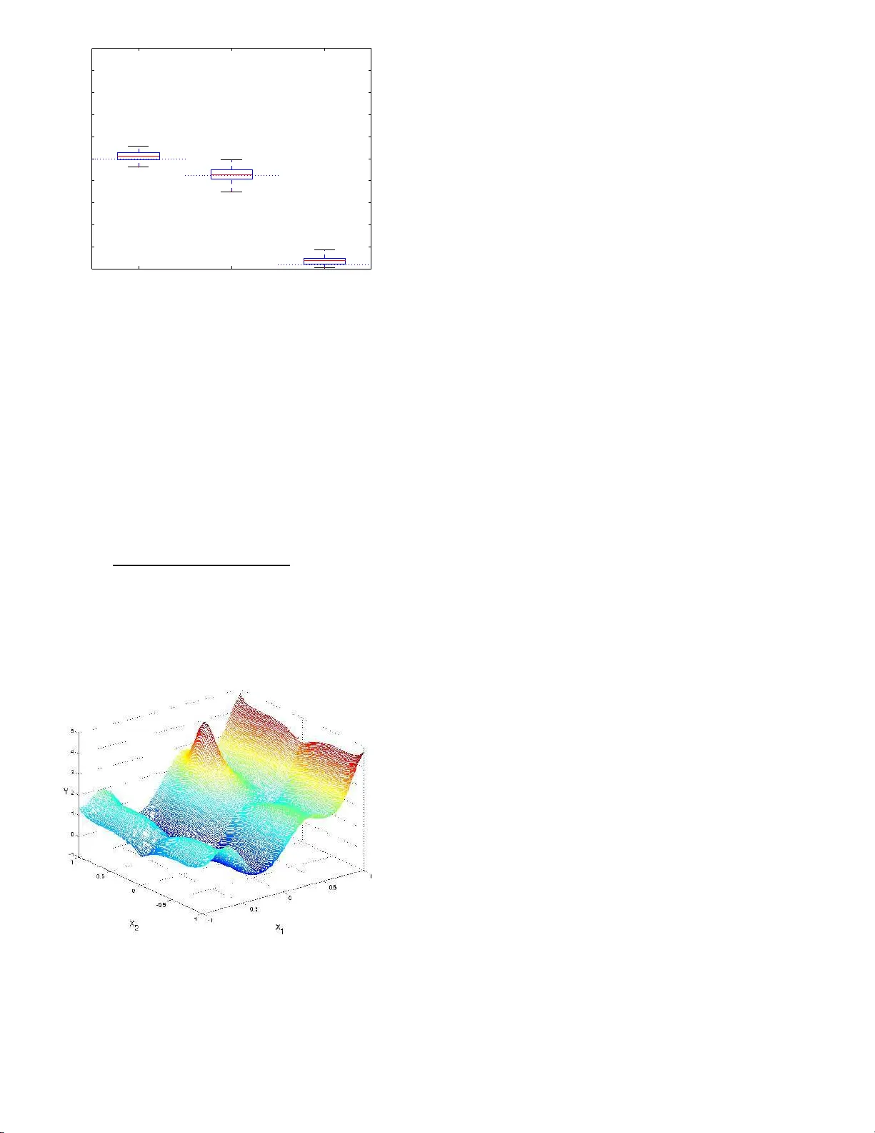
Lo cal P olynomia l Estimatio n for Sensitiv it y Analys is on Mo dels With Correlated Inputs Sebastien D A VE I GA (1) , (2) , F rancois W AHL (1) , F a brice GAMBOA (2) (1) : IFP-Lyon, F rance (2) : Institut de Mathematiques, T oulo use, F ranc e Abstract Sensitivity indices when the in puts of a mo del are not indep endent are estimated by lo cal p olynomial techniques. Tw o original estimators b ased on local p olynomial smo others are prop osed. Both hav e go o d theoretical p rop erties which are exh ibited and also illustrated th rough analytical examples. They are used t o carry out a sensitivity analysis on a real case of a kinetic mo del with correlated parameters. KEY WORDS: Nonp arametric regression; Global sensitivit y indices; Conditional moments estimation. Ac hiev ing b etter knowledge o f refining pro cesses usually re- quires to build a kinetic mo del predicting the output comp o- nent s pro duced in a un it given the input comp onents intro- duced (the “ feed”) a nd the op erating co nditions. Suc h a mo del is based on the choice of a r eaction mechanism dep ending on v a rious para meters ( e.g. kinetic constants). But the complexity of the mechanism, the v ariability of the b ehavior of ca talysts when they are use d and the difficult y of obser v ations and exp er - imen ts imply that most often these pa rameters ca nnot b e in- ferred from theo retical considera tions and need to b e estimated through practical exp eriments. This es timation pro cedure leads to consider them uncertain and this uncertaint y spreads on the mo del predictions. This can b e highly problematic in real sit- uations. It is then esse ntial to quant ify this uncer taint y and to study the influence of parameters v aria tions on the mo del outputs through uncertaint y and sensitivity a nalysis. During the last decades muc h effort in mathematica l analy- sis of ph y sical pro cesses has fo cused o n mo deling a nd reaso ning with uncertaint y and sensitivity . Model calibratio n and v ali- dation are examples wher e sensitivity a nd uncertaint y a nalysis hav e bec ome essential inv estig ative scien tific to ols. Roughly sp eaking, uncer taint y analy sis refers to t he inheren t v aria tions of a mo del ( e.g. a mo deled physical pro ces s) and is helpful in finding the relation betw e e n some v ariability o r pr obability distribution on input para meter s a nd the v a riability and prob- ability distribution o f outputs, while s ensitivity ana lysis inv es - tigates the effects of v arying a mo del input o n the outputs a nd ascertains how muc h a mo del depends on each or s ome of its inputs. Over the years several mathematica l and computer-a ssisted metho ds have been developed to car ry out glo bal sensitivity analysis and the r eader may refer to the b o ok of Sa ltelli, Chan & Sco tt (200 0) for a wide and tho r ough re view. Amongst these metho ds a par ticula r p opular clas s is the one co mp osed by “v ariance-ba sed” metho ds which is detailed b elow. Let us con- sider a mathematical mo del given by Y = η ( X ) (1) where η : R d → R is the mo deling function, Y ∈ R repr esents the output or prediction of the mo del a nd X = ( X 1 , ..., X d ) is the d -dimensional rea l vector o f the input factors or parame- ters. The vector of input parameter s is treated a s a r andom vector, which implies that the output is also a ra ndom v ar iable. In v ar iance-base d metho ds, we ar e in ter ested in explaining the v a riance V ar( Y ) thro ug h the v ariations o f the X i , i = 1 , ..., d and w e deco mp o se V a r( Y ) as follows : V a r( Y ) = V a r( E ( Y | X i )) + E (V ar ( Y | X i )) for all i = 1 , ..., d wher e E ( Y | X i ) and V ar( Y | X i ) are r esp ec- tively the conditiona l exp ectation and v ariance of Y given X i . The imp ortance of X i on the v ariance o f Y is linked to ho w well E ( Y | X i ) fits Y and can then b e mea sured by the first or- der sen s it ivity index S i = V a r( E ( Y | X i )) V a r( Y ) also called c orr elation r atio . W e can also introduce s ensitivity indices of higher order s to ta ke in to account input int e r actions. F o r example, the se c ond or der sensitivity index for X i and X j is S ij = V a r( E ( Y | X i , X j )) − V a r( E ( Y | X i )) − V a r( E ( Y | X j )) V a r( Y ) , and so on for other orders, see Saltelli et al. (200 0) for details. In the case o f indep endent inputs, tw o techniques, Sob ol (Sob o l’ 1993 ) and F AST (Cukier , F ortuin, Sh uler , Petschek & Schaibly 197 3) are the most p opular methods for estimating 1 the S i indices. Althoug h p owerful and computationa lly effi- cient, these metho ds rely on the assumption o f indep e ndent inputs which is hard to hold in many practica l cases fo r ki- netic mo dels. Nevertheless, three origina l metho ds, origina ted by Ratto, T arantola & Saltelli (200 1), Jacques , Lav erg ne & De- victor (2004) a nd Oakle y & O’Haga n (2004), try to deal with this pr oblem. The firs t o ne sets out to calculate the s e nsitivity indices by us ing a replicated latin hypercub e s ampling, but this approach r equires a la rge amount of mo del ev aluations to reach an acce ptable precision. The second one is based on the idea of building new se ns itivity indices which generalize the o rig- inal o nes by tak ing into account blo ck of correlatio ns among the inputs. This metho d is how ever useles s when many input factors are corre lated. The las t a pproach is that of Oakley & O’Hagan (20 04) and rely up on the idea of approximating the function η in mo del (1) by a so -called ’kr iging’ res po nse surface (Sant ner , Williams & Notz 2 003) and o f computing analyti- cal expr essions of the sensitivity indices base d on the results of the krig ing appr oximation. How ever app ealing a nd a ccurate, these analytical expres sions inv o lve multidimensional int e g rals that are only tractable when the conditional densities of the input fa c tors are known and ea sy to integrate. If this is not the case the mult idimensio nal in teg rals must b e approximated nu mer ically , but at high computatio nal cost. W e then prop o se a new wa y of estimating sensitivity indice s throug h an interme- diate technique in the s e nse that it is ba s ed on a sample from the joint densit y of the inputs and the output like Ra tto et a l. (2001) but also on a no nparametric r egress ion mo del like Oak- ley & O’Hagan (200 4). This approach does not requir e as many mo del ev a luations as Ratto et al. (20 01) and do es not r equire to approximate mult idimensio nal integrals as Oakle y & O’Haga n (2004) in the genera l case. In this pa p er to deal with co rrelated inputs we consider a new metho d bas ed on lo cal p olynomial approximations for con- ditional moments (see the work of F an & Gijbels (19 96) and F a n, Gijbels, Hu & Huang (1996) on co nditional exp ectatio n and the pap ers o f F an & Y a o (199 8 ) and Rupp ert, W and, Holst & Hˆssjer (1997 ) o n the conditional v ariance). Given the form of the se ns itivity indices, lo cal po lynomial regr e ssion can b e used to estimate them. This appro a ch no t only allows to com- pute a sens itivity index through an easy black-b ox pr o cedure but also reaches a go od precis ion. The pap er is o rganize d as follows. In Sectio n 1 we r e view the metho ds o f Ratto et a l. (200 1), Ja cques et al. (200 4) and Oakley & O’Hag an (2004 ) and discuss their merits and draw- backs. In Section 2 w e prop ose and study tw o new estimator s for sensitivity indices relying o n lo cal p olynomial metho ds. In Section 3 we present bo th ana ly tical and practical ex amples. In Section 4 we finally give some conclusions and dir ections for future resear ch. 1. MODELS WITH CORRELA TED INPUTS When the inputs are indep endent, Sob ol show ed that the sum of the sensitivity indices of all orders is e q ual to 1, due to a n or- thogonal decomp ositio n of the function η (Sob o l’ 1993 ). Indeed sensitivity indices naturally aris e from this functional ANOV A decomp osition. Nevertheless, when the inputs are cor related, this prop erty do es not hold anymore beca use such a decomp o- sition ca n not be done without tak ing into account the join t distribution o f the inputs. If one decides to e s timate sens itivity indices under the indep endence hypo thesis although it do es not hold, results a nd c o nsequently int er pretation can be higly mis- leading, s e e the first exa mple o f Sec tio n 3.1. But we can s till consider the initial ANOV A deco mp o sition a nd work with the original sensitivity indices without igno ring the correlatio n, and when quantifying the first order sensitivity index o f a particular input factor a part of the sensitivity of all the other input fac- tors correla ted with it is also taken in to account. Thus the s ame information is considered s everal times. Interpretation of s en- sitivity indices when the inputs are no t indep endent b ecomes problematic. Howev er, the input factors b eing indep endent or not, the firs t- order sensitivity index s till p o ints out which factor (if fixe d) will mo stly r educe the v ar iance of the output. Thus, if the goa l of the pra ctitioner is to conduct a ’F actor s P riori- tisation’ (Saltelli, T ara ntola, Camp olo ngo & Ratto 2004 ), i.e. ident ifying the facto r that one should fix to achiev e the gre a test reduction in the uncertaint y of the o utput, first-or der sensitivity indices remain the mea sure of imp or tance to study , s ee Saltelli et al. (2004). Co ns idering that this go al is co mmo n for pra c- titioners, being able to compute first-order sensitivity indices when the inputs are no lo nger indep endent is an interesting challenge. Beyond this problem o f interpretation, cor relation also makes the computational metho ds F AST and Sob ol unusable as they hav e b een designed for the independent case. T o get ov er these difficulties, it is fir st pos s ible to build ’new’ sensitivity indices that would g eneralize the origina l ones a nd match their prop erties, allowing interpretation. This is the idea of multidi- mensional sensitivity ana ly sis of Jac q ues (J a cques et al. 2 004) detailed in the next s ection. Se c o ndly , Ratto et al. (2001 ) tried to co ntin ue o n working with the o riginal sensitivity indices and to compute them as descr ib ed in Section 1.3 , even if they do not give clues for interpretation. The authors gener ate replicated latin hyperc ub e s a mples to approximate conditional densities. Finally , O akley & O’Hagan (20 0 4) s ug gest to a pproach the function η in mo del (1) by a kriging resp onse sur face which a l- lows to get analytical ex pr essions o f sensitivity indices thr ough m ultidimensio nal in teg rals. 1.1 Multidimensional Sensitivity Analys is T o define multidimensional sensitivity indices, Jac ques et a l. (2004) sug gest to split X into p vectors U j , j = 1 , ..., p , each of size k j such that U j is indep endent from U l for 1 ≤ j, l ≤ p , j 6 = l : X = ( X 1 , ..., X d ) = ( X 1 , ..., X k 1 | {z } U 1 , X k 1 +1 , ..., X k 1 + k 2 | {z } U 2 , ... ..., X k 1 + k 2 + ... + k p − 1 +1 , ..., X k 1 + k 2 + ... + k p | {z } U p ) where k 1 + k 2 + .... + k p = d . F o r example, if X = ( X 1 , X 2 , X 3 ) where X 1 is indep endent of X 2 and X 3 but X 2 and X 3 are correla ted, we set U 1 = X 1 and U 2 = ( X 2 , X 3 ). Thu s they build fi rst or der multidimensional sensitivity in- dic es using the U j vectors : 2 S j = V a r( E ( Y | U j )) V a r( Y ) = V a r( E ( Y | X k 1 + k 2 + ... + k j − 1 +1 , ..., X k 1 + k 2 + ... + k j )) V a r( Y ) for j = 1 , ..., p . Remark that if the inputs are indep endent, these sensitivity indices have the sa me expre s sion as in cla ssi- cal sensitivity a nalysis. Finally , it is p oss ible to compute thes e indices by Monte-Carlo estimations. Nevertheless, this metho d has a main drawback hard to ov erco me. If a ll the inputs are correlated, the U j vectors cannot be defined (except the trivial case U 1 = X ) and interpretation is not p os sible. The problem remains the same if to o many inputs ar e dep endent b ecause this situation leads to consider very few multidimensional indices . Mor eov er, identifying a set of co rrelated v ariables U j with high sensitivity index do es not allow to p oint up whether this is due to one particula r input of the set as we cannot differentiate a mong them. W e will illus- trate this phenomenon in the seco nd e x ample of Section 3.1 . 1.2 Correla tion-Ratios Wit h Known Conditional Density F unctio ns The estimator introduced by Ratto et a l. (2001 ) was first dis- cussed in McK ay (1996) and is based on samples fro m the con- ditional density functions o f Y g iven X i , i = 1 , ..., d . Let ( X j ) j =1 ,...,n be an i.i.d sample o f size n from the distri- bution of the vector X . ( X j i ) j =1 ,...,n is then an i.i.d. sample of size n fr om the distr ibution o f the input fac tor X i . F o r each realization X j i of this sample, let ( Y j k i ) k =1 ,..., r be a n i.i.d. s am- ple o f size r from the conditional density function of Y given X i = X j i and define the sa mple mea ns Y j i = 1 r r X k =1 Y j k i Y i = 1 n n X j =1 Y j i . Note that Y j i and 1 r P r k =1 ( Y j k i − Y j i ) 2 resp ectively e stimate the co nditional ex p e ctation E ( Y | X i = X j i ) and the conditio na l v a riance V ar( Y | X i = X j i ), while Y i estimates E ( Y ). Using these moments estimators the numerator of the firs t order sensitivity index S i , V ar( E ( Y | X i )), ca n be estimated by the empirical estimator 1 n n X j =1 ( Y j i − Y i ) 2 . Similarly the denominator o f S i , V ar( Y ), is estimated by 1 n n X j =1 1 r r X k =1 ( Y j k i − Y i ) 2 . The estimator of the first order sensitivity index S i of the input factor X i , i = 1 , ..., d is then defined a s ˆ S i = S S B S S T where S S B = r n X j =1 ( Y j i − Y i ) 2 and S S T = n X j =1 r X k =1 ( Y j k i − Y i ) 2 . T o compute these indices and to gene r ate the sa mples needed, Ratto uses tw o different metho ds : pure Monte-Carlo s ampling and a single replicated Latin Hyp erCub e (r - LHS) sampling. It is c rucial to note, how ever, that these tw o methods r equire a huge a mount of mo del ev aluations to reach a go o d precisio n and ca n only b e used fo r ca ses where mo del runs have very low computational cost. 1.3 Bay esian Sens itivit y Analysis The idea of Oakley & O ’Hagan (2004) is to see the function η ( · ) as a n unknown smo oth function and to formulate a prio r dis- tribution for it. More precise ly , it is mo deled as the realiza tion of a Gaussian stationa ry random field with g iven mean and co - v a riance functions. Then, g iven a set of o f v alues y i = η ( x i ), we can derive the po sterior distribution of η ( · ) b y classical Bay esian consideratio ns. The prior distribution of η ( x ) is a Gaus sian s ta- tionary field : η ( x ) = h ( x ) t β + Z ( x ) conditionally on β and σ 2 , wher e h ( · ) is a vector of q known regres s ion functions and Z ( X ) is a Gaussian stationary random field with z ero mean a nd cov ariance function σ 2 c ( x , x ′ ). The vector h ( · ) and the corr elation function c ( · , · ) a r e to b e chosen in order to inco r p orate some informatio n abo ut how the o utput resp onds to the inputs and ab out the amount of smoo thness we r e quire on the output r e s p ectively . W e refer the re ader to Santner et al. (2 003) a nd to Kennedy & O ’Ha gan (20 01) for a detailed discussio n on these choices. The second sta ge prior concerns the conjugate prio r form for β and σ 2 , which is chosen to b e a normal in verse gamma distribution. Now a ssuming we observe a set y of n v a lues of y i = η ( x i ), we can derive that the p oster ior distr ibution of η ( · ) given these data is a Student distribution, see Oakley & O’Haga n (20 0 4) for details. Using this p osterio r distribution, sensitivity indices can b e co m- puted analytica lly through multidimensional in tegr als inv olving functions of the observ atio ns and the conditiona l distributions of the input fa c tors only . The main adv antage of this Bay esia n approach is that the mo de l is only ev aluated to calcula te the quantities a b ove, i.e. to ’fit’ the resp onse surfac e . Once this is done the estimation of sensitivity indices just inv o lves the conditional distributions of the input fac to rs. When the num- ber of mo del runs is fixed, this metho d clear ly reduces the standard er rors of the estimated se nsitivity indices obtained by Monte-Carlo metho ds such as Sobo l (when the input factors are indep e ndent ) and ca n still b e used when the input factor s are not indepe ndent . How ever, the m ultidimensiona l integrals leading to the com- putation of the sensitivity indices , if no t tractable analytically , need to b e es timated. Let us descr ib e mo r e pa rticularly one 3 of the es timators prop osed in Oa kley & O’Hag an (2 0 04). W e keep the author s notations and denote b y E ∗ the exp ectations defined with resp ect to the p osterior distribution o f η ( · ). The nu mer ator o f the first-order sens itivit y index of Y with resp ect to X 1 is estimated by E ∗ (V ar( E ( Y | X 1 ))) = E ∗ ( E ( E ( Y | X 1 ) 2 )) − E ∗ ( E ( Y ) 2 ) and one of the quan tities inv olved in the computation of E ∗ ( E ( E ( Y | X 1 ) 2 )) is for example U 1 = Z R d − 1 Z R d − 1 Z R c ( x , x ∗ ) d F − 1 | 1 ( x − 1 | x 1 ) d F − 1 | 1 ( x ′ − 1 | x 1 ) d F 1 ( x 1 ) where F − 1 | 1 is the margina l distribution o f X − 1 (subv ector of X c o ntaining a ll element s except X 1 ) given X 1 , F 1 is the marginal dis tribution of X 1 and x ∗ denotes the vector with ele- men ts made up o f x 1 and x ′ − 1 in the same wa y as x is co mp o sed of x 1 and x − 1 . If the co nditional distribution F − 1 | 1 is not a n- alytically known, we first nee d to es timate it with a sample of the joint distribution F . Many metho ds hav e b een develop ed to do so, let us just ment io n for example kernel techniques. But in general in high dimension the data is very sparsely distributed and it is difficult to g et an accura te appr oximation of condi- tional distributions since the so- c a lled cur se of dimensionality arises. F or instance the b est p ossible MSE r a te with kernel techn iq ues is n − 4 / (4+ d ) which b ecomes worse a s d gets larger . Moreov e r , even if we could get a go o d appr oximation of F − 1 | 1 , still r e mains the problem of ev aluating the multidimensional int eg rals. Indeed the dimensio na lity of these integrals can reach 2 d − 1 as in the expressio n of U 1 ab ov e. Since these int eg rals can not in general b e separated in to unidimensiona l int eg rals, approximating them with a sufficent accura cy is not an obvious mathematica l problem. Deterministic schemes ca n not rea sonably b e cons ider ed, and with Mo nte-Carlo or q uasi Monte-Carlo sampling (O wen 20 05) thousa nds (or millio ns) of draws are requir ed to g et a reaso nable accura cy . With unknown densities, even if conceptually , sampling rather than a na lytical integration in the Oakle y and O’Haga n approach seems reaso nable, the results could be highly af- fected b y the curse of dimensionality . Let us mention that P r. O’Hagan has public do main softw are carr ying o ut this analysis . How ever it do es not yet allow to consider dep endent inputs. 2. NEW ESTIMA TION METHODOLOG Y Our appro ach is to estimate the conditiona l moments E ( Y | X i = X j i ) and V ar ( Y | X i = X j i ) with an intermediate metho d b e- t ween the o ne of Ratto et al. (20 01) and Oa kley & O’Hag an (2004). W e firs t us e a sample ( X i , Y i ) to estimate the co ndi- tional moments with nonpar ametric to ols (provided they ar e smo oth functions of the input facto rs). Then, w e compute sensitivity indices by using ano ther sa mple of the input factors only (and thus no more mo del r uns are needed). While O akley & O ’Hagan (200 4 ) approximate the function η ( X ) in R d , we approximate it marginally , i.e. w e approximate the conditiona l exp ectations E ( η ( X ) | X i ) in R . This approa ch a llows to ov er- come the multidimensional integration problem of the Bayesian sensitivity analys is . T o simplify the nota tions, unt il Sec tio n 2.4 ( X, Y ) will stand for a biv aria te rando m vector ( i.e. X is unidimen- sional). A s the v arianc e may b e decomp osed as V ar( Y ) = V a r( E ( Y | X )) + E (V ar ( Y | X )), the index we wish to estimate can be written S = V a r( E ( Y | X )) V a r( Y ) or S = 1 − E (V ar ( Y | X )) V a r( Y ) . (2) These expr essions cle a rly give tw o wa ys of es timating S : the issue is to be able to estimate V ar( E ( Y | X )) or alternatively E (V ar ( Y | X )), o bviously by estimating first the conditio na l mo- men ts E ( Y | X = x ) and V ar ( Y | X = x ) ( x ∈ R ). I n b o th cases the denominato r term V ar( Y ) can be easily estimated. T o ap- proximate the conditional moments, we prop ose to use lo cal po lynomial r egress io n. This highly sta tistical efficien t to ol is easy to apprehend as it is close to the weigh ted least-squa res approach in r egress ion problems. Only basic res ults will b e pr e- sented here, for a detailed picture of the sub ject the interested reader is referred to F an & Gijb els (199 6). 2.1 F o rmulation of the Estimato rs Let ( X i , Y i ) i =1 ,...,n be a tw o-dimensio nal i.i.d. sample of a real random v ec tor ( X , Y ). Assuming that X and Y are sq uare in- tegrable we may write an hetero skedastic re g ressio n mo del of Y i on X i , exhibiting the conditional exp ectation and v a riance, as Y i = m ( X i ) + σ ( X i ) ǫ i , i = 1 , . . . , n where m ( x ) = E ( Y | X = x ) a nd σ 2 ( x ) = V ar ( Y | X = x ) ( x ∈ R ) are the co nditional moments a nd the err o rs ǫ 1 , . . . , ǫ n are indep e ndent random v ariables sa tis fying E ( ǫ i | X i ) = 0 and V a r( ǫ i | X i ) = 1. Usua lly ǫ i and X i are assumed to b e inde- pendent although this is not the case in o ur work. Note that results for corr elated erro rs hav e b een recently dev elo p ed (Vilar- F er n´ andez & F rancisco- F ern´ andez (2002) for the autor egress ive case fo r example). L o cal p olynomial fitting consists in approx- imating lo c al ly the regr e ssion function m by a p -th o rder po ly- nomial m ( z ) ≈ p X j =0 β j ( z − x ) j for z in a neighbor ho o d of x . This p olynomial is then fitted to the obser v ations ( X i , Y i ) by solving the weight e d least-squar es problem min β n X i =1  Y i − p X j =0 β j ( X i − x ) j  2 K 1  X i − x h 1  (3) where K 1 ( . ) denotes a kernel function and h 1 is a smo oth- ing parameter (or b andwidth ). In this case, if ˆ β ( x ) = ( ˆ β 0 ( x ) , ..., ˆ β p ( x )) T denotes the minimizer of (3) we have ˆ m ( x ) = ˆ β 0 ( x ) , while the ν -th deriv ative of m ( x ) is e s timated via the relation ˆ β ν ( x ) = ˆ m ( ν ) ( x ) ν ! , 4 see F an & Gijbels (1996) for more details. As it will b e dis- cussed later, the s mo othing parameter h 1 is chosen to bala nce bias and v ariance of the estimator. Fina lly , remar k that the particular case p = 0 (consta nt fit) leads to the well-kno wn Nadar aya-Watson estimator ˆ m N W ( x ) of the conditional exp ec- tation, given explic itly by ˆ m N W ( x ) = n X i =1 Y i K  X i − x h  n X i =1 K  X i − x h  , see W a nd & Jo ne s (1994 ). Estimation of the conditional v ar ia nce is less straightfor- ward. If the regressio n function m was known, the prob- lem o f estimating σ 2 ( . ) would b e rega rded as a local p oly- nomial regr ession of r 2 i on X i with r 2 i = ( Y i − m ( X i )) 2 , as E ( r 2 | X = x ) = σ 2 ( x ) with r 2 = ( Y − m ( X )) 2 . But in practice, m is unknown. A natural approach is to substitute m ( . ) by its estimate ˆ m ( . ) de fined a s ab ove a nd to g et the the r esidual- b ase d estimator ˆ σ 2 ( x ) by s olving as previously the weigh ted least-squar es problem min γ n X i =1  ˆ r 2 i − q X j =1 γ j ( X i − x ) j  2 K 2  X i − x h 2  (4) where ˆ r 2 i = ( Y i − ˆ m ( X i )) 2 , K 2 ( . ) is a kernel and h 2 a smo othing parameter. Note that the kernel K 2 ( . ) is not neces sarily chosen to b e equal to the kernel K 1 ( . ). The n ˆ σ 2 ( x ) = ˆ γ 0 ( x ) where ˆ γ ( x ) = ( ˆ γ 0 ( x ) , ..., ˆ γ q ( x )) is the minimizer o f (4). As pre- viously , the smo othing parameter h 2 has to b e chosen to ba lance bias and v ariance of the estimator , see F a n & Y ao (1998 ). Going back over the equa lities in (2), the la s t step is to es- timate the qua ntit ies V a r( E ( Y | X )) and E (V ar( Y | X )) b y using the lo ca l p olynomia l estimators for the conditional moments defined r ight ab ove. T o do this let us as s ume we have an- other i.i.d. s ample ( ˜ X j ) j =1 ,...,n ′ with sa me distribution a s X . If the functions m ( . ) and σ 2 ( . ) were known, we could estimate V a r( E ( Y | X )) = V ar( m ( X )) and E (V ar( Y | X )) = E ( σ 2 ( X )) with the classica l empirica l momen ts 1 n ′ − 1 n ′ X j =1  m ( ˜ X j ) − ¯ m  2 and 1 n ′ n ′ X j =1 σ 2 ( ˜ X j ) where ¯ m = 1 n ′ n ′ X j =1 m ( ˜ X j ). As m ( . ) and σ 2 ( . ) are unknown, the main idea is to r e place them b y their lo cal po lynomial es tima- tors which leads to cons ider ˆ T 1 = 1 n ′ − 1 n ′ X j =1  ˆ m ( ˜ X j ) − ˆ ¯ m  2 and ˆ T 2 = 1 n ′ n ′ X j =1 ˆ σ 2 ( ˜ X j ) where ˆ ¯ m = 1 n ′ n ′ X j =1 ˆ m ( ˜ X j ) and ˆ m ( . ) and ˆ σ 2 ( . ) are the lo cal p oly- nomial estimato r s of m ( . ) a nd σ 2 ( . ) introduced ab ove. It is impo rtant to note that we nee d tw o samples, the first one ( X i , Y i ) i =1 ,...,n to compute ˆ m ( . ) and ˆ σ 2 ( . ) a nd the second one ( ˜ X j ) j =1 ,...,n ′ to finally compute the empirical e s timators ˆ T 1 and ˆ T 2 . 2.2 Bandwidth and Orders Selection The selection of the smo othing parameters h 1 and h 2 and to a lesser extent of the p olynomials o rders p a nd q ca n b e crucia l to get the least mean squared err or (MSE) o f the es timators ˆ T 1 and ˆ T 2 . Classically the MSE co nsists of a bias term plus a v aria nce term and so is minimized by finding a compromise betw e e n bia s and v ariance. Concerning this choice, the reader is r eferred to F an et al. (1996), F an & Y ao (199 8) or Rupp ert (1 9 97). Most of the meth- o ds sugges ted by these authors rely upon a s ymptotic arg uments and their efficiency for finite sample ca ses is not clear. In prac- tice cross -v alidation metho ds can b e used for the finite sample case (Jones, Marro n & Shea ther 199 6), but in the examples of Section 3 we will use the empirica l-bias bandwidth selecto r (EBBS) of Rupp e r t which app ears to b e efficient on simulated data. EBB S is based o n estimating the MSE empirica lly and not with an asymptotic expr ession. The choice of the p olyno- mials order s is mo re s ub jectiv e. Concerning the estima tio n of the conditional exp ectatio n, F a n & Gijb els (1996) r ecommend to use a ν + 1 or ν + 3 th-order p olynomia l to estimate the ν th- deriv ative of m ( x ), following theor etical consider ations on the asymptotic bia s o f ˆ m ( x ) on the b oundar y . W e would then be lead to take p = 1 or p = 3 to es timate the 0th-de r iv ative m ( x ). But Rupp ert, W and & Car r oll (200 3) sugges t that this conclu- sion sho uld be balanced by simulation studies a nd stress that p = 2 often outp erforms p = 1 and p = 3. The only common conclusion is tha t lo ca l linear regr ession ( p = 1) is usually sup e- rior to kernel regres sion (Nadaraya-W atso n estimator obtained with p = 0). This is the reason why we will only consider a nd study lo cal linear regr ession for m ( x ) in the next theor etical and practical sections. The choice is s till difficult when es tima ting the co nditional v ariance as we hav e to choose p and q simul- taneously . One more time, the authors are not una nimous : F a n & Y ao (199 8 ) recommend the case p = 1 , q = 1 whereas Rupper t et al. (1997) suggest p = 2 , q = 1 or p = 3 , q = 1 . How ever on the simulations we hav e carrie d out, the choice of p = 1 , q = 1 is ade q uate and sa tisfactory in terms of precision. This is the reason why w e hav e decided to consider only the case p = 1 , q = 1 for bo th theoretical and practica l results. 2.3 Theoretical Prop er ties of the Estimators The prop erties of ˆ T 1 and ˆ T 2 strongly dep end o n the asymp- totic results on the bias and v ariance of the lo c a l linear esti- mators ˆ m ( . ) and ˆ σ 2 ( . ). W e o nly g ive here tw o main results, all assumptions ( A 0 , ..., A 4 , B 0 , ..., B 4 , C 0 ) and pro ofs are given in app endix for re adability . E X and V ar X stand for the co nditional exp ectation and v a riance given the predictors X = ( X 1 , ..., X n ). The expression o P ( ϕ ( h )) is equal to ϕ ( h ) o P (1) for a given func- tion ϕ . Her e o P (1) is the standar d notation for a sequence of random v ar iables that conv erg es to zero in pro ba bility . Theorem 1 Under assumptions (A 0)-(A4) and (C0), the es- timator ˆ T 1 is asymptotic al ly u nbiase d. Mor e pr e cisely 5 E X ( ˆ T 1 ) = V ar ( E ( Y | X )) + M 1 h 2 1 + M 2 nh 1 + o P ( h 2 1 ) . wher e M 1 and M 2 ar e c onst ants given in app endix. R emark 1. It would be interesting to calculate the v ar iance of this e stimator, but it would re quire the expr essions of the third and fourth moments of the lo cal linear estimato r ˆ m ( . ) (see the app endix). This is not a n obvious proble m and to the bes t of our k nowledge it has not been addressed in the liter - ature. It is b eyond the scop e of the present paper but it is an interesting problem for future research. Nev ertheless , the v a riance ca n b e estima ted on practical c ases thro ugh b o otstra p metho ds for example (Efron & Tibshirani 1994 ). Theorem 2 Under assumptions (B0)-(B4) and (C0), the es- timator ˆ T 2 is c onsistent. Mor e pr e cisely E X ( ˆ T 2 ) = E ( V ar ( Y | X )) + V 1 h 2 2 + o P ( h 2 1 + h 2 2 ) and V ar X ( ˆ T 2 ) = 1 n ′  E ( V ar ( Y | X ) 2 ) + V 2 h 2 2 + V 3 h 2 1 + V 4 nh 2 + o P  h 2 1 + h 2 2 + 1 √ nh 2  wher e V 1 , V 2 , V 3 and V 4 ar e c onst ants given in app endix. 2.4 Application to Sensitivity Analy sis Let us come back to the mo del (1), where X is mult idimen- sional. The goa l is to get an estimate of S i for i = 1 , . . . , d by using one of the t wo es timators ˆ T 1 and ˆ T 2 . W e need t wo sa mples to compute ea ch of them, i.e. a sample ( X k i , Y k ) k =1 ,..., n to esti- mate ˆ m ( . ) a nd ˆ σ 2 ( . ) and a sample ( ˜ X l i ) l =1 ,...,n ′ to get ˆ T 1 and ˆ T 2 where ( X k i ) k =1 ,..., n and ( ˜ X l i ) l =1 ,...,n ′ are samples from the joint distribution of the d -dimensional input factors X = ( X i ) i =1 ,...,d and ( Y k ) k =1 ,..., n a sample of the output Y . Note that the mo del is run just for the first sample a nd not for the seco nd one. Three situations can ar ise : 1. Sampling fro m the joint distribution of X has lo w computational cost a nd running the mo del to co mpute ( Y k ) k =1 ,...,n is cheap. This is the ideal situa tion. In- deed in this case the tw o s amples ( X k i , Y k ) k =1 ,..., n and ( ˜ X l i ) l =1 ,...,n ′ can b e g e ne r ated independently and b e as large as required ; 2. Sampling fr om the join t distribution of X has low com- putational cost but mo del ev aluatio ns hav e not. In this case (also po inted o ut by Oakley & O’Hagan (20 0 4)) a mo derate-size d sample ( X k i , Y k ) k =1 ,...,n is used in order to fit the co nditional mo ments. How ever to c ompute ˆ T 1 and ˆ T 2 we can then us e a sample ( ˜ X l i ) l =1 ,...,n ′ of larg e size ; 3. Sampling from the joint distribution of X has high co mpu- tational cost. This case can ar ise in practice for e x ample when the input factors are obtained throug h a pro cedure based on exp erimental data and optimizatio n r o utines. W e then have an initial sample ( X j ) j =1 ,...,N of limited size N that we wish to use for the tw o steps o f the esti- mation. The first idea is to split it and to use the firs t part to get the s ample ( X k i , Y k ) k =1 ,..., n and the second one to get ( ˜ X l i ) l =1 ,...,n ′ . The drawbac k of this metho d clear ly arises if N is very small. Another wa y to tackle the pr o b- lem is to use the well-kno wn leave-one-out idea pro cedure which gives b etter a pproximation than data splitting. As sugg ested by the Asso c ia te Editor a nother p o ssible metho d could be to use the sa mple of size N to esti- mate the conditional moments and to estimate also the marginal densities of each input using for insta nce a non- parametric density estimator . One could then use these density estimates to get the sample ( ˜ X l i ) l =1 ,...,n ′ . The clear disadv ant a ge o f this pro cedure is that it may bias the fina l estimators. So me simulation r uns not r ep o rted here for la ck of space show that such a pro cedur e leads to less efficient estimates pro bably due to the lar ge bias pro duced by nonpa rametric metho ds. The la st situatio n obviously le ads to the less accur ate ap- proximations of firs t-order sensitivity indices. How ever in g en- eral, litterature and r esults o n sensitivity analy sis assume tha t, if not a nalytically k nown, the joint distribution of the input fac- tors can at least b e generated at low computatio nal cost. This is the r e ason why we will only describ e here the pro cedure for estimating fir st-order sensitivity indices in ca se 1 or 2. W e now assume tha t we have tw o samples ( X k i ) k =1 ,..., n and ( ˜ X l i ) l =1 ,...,n ′ obtained by one of the metho ds desc r ib ed right ab ov e. The estimatio n pro cedure fo r S i = V a r( E ( Y | X i )) V a r( Y ) is the follow- ing : Step 1 : Co mpute the o utput sample ( Y k ) k =1 ,..., n by run- ning the mo del at ( X k ) k =1 ,..., n Step 2 : Compute ˆ σ 2 Y , the cla ssical un bia sed estimator of the v ar iance V a r( Y ) ˆ σ 2 Y = 1 n − 1 n X k =1  Y k − ¯ Y  2 Step 3 : Use the s a mple ( X k i , Y k ) k =1 ,..., n to obtain ˆ m ( ˜ X l i ) for l = 1 , . . . , n ′ and ˆ m ( X k i ) for k = 1 , . . . , n using the smo oth- ing parameter h 1 given by EBBS Step 4 : Compute square d r esiduals ˆ r k = ( Y k − ˆ m ( X k i )) 2 for k = 1 , . . . , n and a pply the smo othing pa rameter h 2 obtained by EBBS to compute ˆ σ 2 ( ˜ X l i ) for l = 1 , . . . , n ′ Step 5 : Compute ˆ T 1 with ˆ m ( ˜ X l i ) for l = 1 , . . . , n ′ from Step 3 and compute ˆ T 2 with ˆ σ 2 ( ˜ X l i ) for l = 1 , . . . , n ′ from Step 4 Step 6 : The estimates of S i are then ˆ S (1) i = ˆ T 1 ˆ σ 2 Y and ˆ S (2) i = 1 − ˆ T 2 ˆ σ 2 Y . (5) 6 T o o btain all the first-o rder sens itivity indices, rep e a t the pro cedure from Step 3 to Step 6 for i = 1 , ..., d . R emark 2. Given the theoretical prop erties o f ˆ T 1 and ˆ T 2 and more precis e ly their non-par a metric co nv ergenc e rate, we can also exp ec t a nonpara metric co nv ergence rate for ˆ S (1) and ˆ S (2) . R emark 3. In pra ctice, our simulations show that n o f the order o f 1 00 and n ′ around 20 00 ar e enough for accurate es ti- mation of the sensitivity indices. 3. EXAMPLES In all the following examples we us e the t wo estimators ˆ S (1) and ˆ S (2) defined in (5). As mentioned in Sectio n 2.2, the condi- tional ex p e ctation is estimated her e with lo ca l linea r r e gressio n ( p = 1) and the conditional v ar iance with p = 1 and q = 1, the bandwidths b eing selected by the estimated-bias metho d of Rupper t (1997 ). 3.1 Analytical Exa mples In this s ection, we car ry out tw o different co mparisons in or der to study our tw o estimators from a numerical p oint o f view. The first mo del has b een chosen to underline their pr ecision in correla ted cases when F AST a nd Sob ol metho ds are no longer efficient and when J acques’ approa ch for multidimensional sen- sitivity analys is is limited. W e als o show how in terpr etation with s e ns itivity indices o btained by neglecting corr elation can be false. The second one is an example illustrating the p erfor- mance of our estimator s with resp ect to the metho d of O akley and O’Haga n in a tw o- dimensional setting. In the first analytical example, we s tudy the mo del Y = X 1 + X 2 + X 3 where ( X 1 , X 2 , X 3 ) is a three-dimens ional norma l vector with mean 0 and cov aria nce matrix Γ =   1 0 0 0 1 ρσ 0 ρσ σ 2   where ρ is the corr elation of X 2 and X 3 and σ > 0 is the stan- dard dev iation o f X 3 . The first order sensitivity indices can b e ev aluated analytica lly : S 1 = 1 2 + σ 2 + 2 ρσ S 2 = (1 + ρσ ) 2 2 + σ 2 + 2 ρσ S 3 = ( σ + ρ ) 2 2 + σ 2 + 2 ρσ The first crucial remar k to be done in this case is that we must take int o account corr elations to e s timate sensitivity indices if we wan t a se rious in vestigation of this mo del. Indeed, let us consider the case where σ = 1 . 2 and ρ = − 0 . 8. W e then hav e S 1 = 0 . 65 79 , S 2 = 0 . 00 11 , S 3 = 0 . 1053 , indicating that X 1 should b e the input to b e fix e d to reach the higher v aria nce r eduction o n Y . But if one neglects the corr e - lation, by computing for insta nc e these indices with the F AST metho d, i.e. working with a thr ee-dimensional no r mal vector with mean 0 and c ov ariance matrix I instead of Γ, one would estimate S 0 1 = 0 . 29 07 , S 0 2 = 0 . 2907 , S 0 3 = 0 . 4186 where S 0 stands for the sensitivity indices when ρ = 0. These results indicate that X 3 should b e fixed to mostly reduce the v a riance of Y , which is absolutely wrong a s the calculations ab ov e hav e shown. This simple exa mple highlights the da n- ger o f neg lecting the corr elations b etw een the inputs and the impo rtance to take them in to co nsideration when computing sensitivity indices. Otherwise, applying Jac q ues’ idea to X 1 and the couple ( X 2 , X 3 ), we also get the e x pression of the firs t order multi- dimensional sensitivity index S { 2 , 3 } = 1 + σ 2 + 2 ρσ 2 + σ 2 + 2 ρσ Cho osing ρ = − 0 . 2 and σ = 0 . 4, w e hav e S 1 = S { 2 , 3 } = 0 . 5 , S 2 = 0 . 42 32 , S 3 = 0 . 02 If w e interpret these indices as suggested by Ja cques’ multidi- mensional sens itivity analysis , the o nly conclusio n we can give is that the couple ( X 2 , X 3 ) has the s ame impo rtance as X 1 . Indeed S { 2 , 3 } = S 1 . But a c tua lly the high v alue of S { 2 , 3 } comes from X 2 as s hown by the exa ct calcula tions a b ove, which im- plies that the information on S { 2 , 3 } alone is not sufficient. But with our metho d, w e can estimate a ll the first or der sensitivity indices : ˆ S (1) 1 = 0 . 48 95 , ˆ S (1) 2 = 0 . 42 50 , ˆ S (1) 3 = 0 . 0234 ˆ S (2) 1 = 0 . 50 81 , ˆ S (2) 2 = 0 . 43 68 , ˆ S (2) 3 = 0 . 0361 for an average up on 1 00 simulations with n = 5 0 and n ′ = 100 0. W e display in Figur e 1 the b oxplots corr e sp onding to the distri- bution of the sensitivity indices on these 100 simulations with the es tima to r ˆ T 2 . B e c ause o f the mathematical complexity men- tioned b efore for the computatio n of the v aria nce of ˆ T 1 , we ar e not able to recommend one estimator over the other one from a theo retical p oint o f view. B ut in practice, we hav e obs erved that the v ariance of ˆ T 2 is at leas t compar able to the v ariance of ˆ T 1 , and sometimes low er. Nervertheless, the computatio n o f ˆ T 2 is more difficult as illustra ted in Section 2.4. 7 1 2 3 0 0.1 0.2 0.3 0.4 0.5 0.6 0.7 0.8 0.9 1 Sensitivity index Input factor Figur e 1. Boxplot of the estimate d sensitivity i ndic es ( ˆ S (2) ) f or the thr e e-factor additive mo del, 100 simulations. Dot li nes ar e the true values . Computing S 2 and S 3 with our metho d, even if b oth o f them take into account c o rrela tio ns, allows to confir m the ex - pec ted r esult : all the v ariability comes from X 2 , and not fr o m X 3 . This simple example then brings out the limitation of the m ultidimensio nal appro ach. In the second analytical example we conside r the mo del Y = 0 . 2 exp( X 1 − 3) + 2 . 2 | X 2 | + 1 . 3 X 6 2 − 2 X 2 2 − 0 . 5 X 4 2 − 0 . 5 X 4 1 + 2 . 5 X 2 1 + 0 . 7 X 3 1 + 3 (8 X 1 − 2) 2 + (5 X 2 − 3) 2 + 1 + sin(5 X 1 ) cos(3 X 2 1 ) where X 1 and X 2 are independent random v ar iables unifor mly distributed o n [ − 1 , 1]. Such a mo del is routinely used at Insti- tut F r ancais du Petrole to compar e different res po nse surface metho dologies as it pr e s ents a p ea k and v alleys. The function is plotted in Figur e 2. Figur e 2. F unction pr op ose d in mo del 2 . In this case, the sensitivity indices a re S 1 = 0 . 93 75 and S 2 = 0 . 0625 W e considered a 6 × 6 regular grid on [0 , 1 ] 2 and used it to estimate the p o s terior distribution in the metho d o f Oakley and O’Hagan and to es timate the conditiona l moments in o ur metho d. Then, we c alculated analytically the m ultidimensional int eg rals in the Bayesian appro ach while using a sample o f size 5000 to compute ˆ S (2) i for i = 1 , 2. The B ayesian appro a ch leads to ˆ S 1 = 0 . 90 38 and ˆ S 2 = 0 . 09 61 while the lo cal p o lynomial technique g ives ˆ S (2) 1 = 0 . 9127 and ˆ S (2) 2 = 0 . 04 52 . W e can see on this example that the results obtained with b oth metho ds ar e compar able. How ever o n this simple ca se the mul- tidimensional integrals were analytica lly computed, which co uld not b e the case in a non- indepe ndent setting. If no t, a numerical int eg ration, if feasible, would lea d to le s s a ccurate approxima- tions as discussed in Section 1.3. 3.2 Practica l Example fro m Chemical Field : Isomeriz a tion of the Normal Butane The iso merization of the no rmal butane, i.e. mole c ules with four carb o n a toms, is a chemical pro cess aiming at tra nsforming normal butane (nC4) int o iso-butane (iC4) in order to obta in a higher o ctane num b e r, favored by iC. A s implified reaction mechanism has b een used : nC4 ← → iC4 (1) 2 iC4 − → C3+C5 (3) nC4 + iC4 − → C3+C5 (4 ) where reac tion (1) is the main re versible reaction c o nv erting the normal butane into iso- butane. Reactions (3) and (4) are se c- ondary a nd irreversible rea ctions which pr o duce propane (C3) and a lump of normal and iso-p entane (C5), par affins with three and five ca rb on a toms. The mo del linked to this pro cess ca n be written as Y = η ( c , θ ) where - Y is the 3 -dimensional result vector (mole fr actions of the comp onents nC4, iC4, C3 and C5 ; note that their sum is 1), - c is the vector c o ntaining the op er ating conditions (pres- sure, temper ature,...) and the mole frac tion o f the input co m- po nents (nC4 and iC4, this is ca lled the fe e d ), - θ = ( θ i ) i =1 ,..., 8 is the 8-dimensiona l random vector of the parameters of the re a ctions (pre-e xp onential fa ctors, activ ation energies, adsorption constants,...), - f is the function mo deling the chemical reactor in which the r eaction takes pla ce. It is ev aluated throug h the res olution of an ordinar y differential equatio ns system which can not b e analytically solved and is calculated numerically . The first step here is to get the dis tribution of θ which is unknown. How ever, it is pos sible to use the e x p e rience and the knowledge of chemical eng ineers to suggest a reasonable a pprox- imation of this distributio n. Class ically , we assume that θ has a m ultiv aria te Gaussian distribution with mean ze r o (once the 8 parameters are centered). Concerning the co r relation ma trix, it is built with exp er ts and with the help of b o otstra p sim ulatio ns and is given by : Γ = 2 6 6 6 6 6 6 6 6 6 4 1 0 . 43 0 . 09 0 . 29 0 . 55 0 . 66 0 . 10 − 0 . 01 0 . 43 1 − 0 . 54 0 . 11 0 . 37 0 . 25 0 . 51 − 0 . 48 0 . 09 − 0 . 54 1 − 0 . 02 0 . 20 0 . 02 − 0 . 40 0 . 73 0 . 29 0 . 11 − 0 . 02 1 − 0 . 41 − 0 . 07 − 0 . 22 0 . 01 0 . 55 0 . 37 0 . 20 − 0 . 41 1 0 . 43 0 . 31 0 0 . 66 0 . 25 0 . 02 − 0 . 07 0 . 43 1 0 . 17 − 0 . 11 0 . 10 0 . 51 − 0 . 40 − 0 . 22 0 . 31 0 . 17 1 − 0 . 61 − 0 . 01 − 0 . 48 0 . 73 0 . 01 0 − 0 . 11 − 0 . 61 1 3 7 7 7 7 7 7 7 7 7 5 In order to compute s e ns itivity indices, we genera te a sample of size n = 5 000 fro m this distribution. Here we wish to estimate, for a given op era ting conditions and feed vector c , the sensitivity indices o f the outputs with res p e c t to the input factors in θ , i.e. S j i = V a r( E ( Y j | θ i )) V a r( Y j ) for j = 1 , ..., 3 and i = 1 , ..., 8 . Actually , o ur goa l is to iden tify on which factor we should make the effort of reducing the un- certaint y , by carrying out new exper iments. This factor should be chosen in o rder to reduce as m uch as p o ssible the uncertaint y of the outputs. W e consider tw o par ticular vectors c 1 and c 2 containing the same op era ting c o nditions but a different feed ( c 1 : nC4=1 and iC4=0, c 2 : iC4= 1 a nd nC4=0 ). W e hav e dr awn fo r ea ch vector c i , i = 1 , 2 a sample of siz e n from Y b y Monte-Carlo simulations, i.e. by computing Y j = η ( c i , θ j ) for j = 1 , ..., n . Thu s we have a sample from ( Y , θ ) for each par ticula r c 1 and c 2 . F or insta nc e , the estimates of the sensitivity indices o f the third output C3+C5 with the ˆ T 1 estimator are g iven in Figure 4. Filled bars corres p o nd to c 1 and empt y bars to c 2 . Note that the estimates given by the ˆ T 2 estimator are simi- lar. These re sults highlight the b ehavior of the C3+ C5 o utput when the feed changes. Indeed when we only use nC4 in the feed ( c 1 ) the pro duction of C3+ C5 is mainly linked to the pro duction of iC4 by rea ction (1). This is confirmed by the impo rtance of par ameters 1 and 6 in Figure 4 which are the parameters inv olved in rea ction (1). When the feed only con- tains iC4 ( c 2 ), the first rea c tio n is no long er dominating fo r the pr o duction of C3+C5, now mainly linked to r eaction (3). Parameters 4 and 2 that a re the mo st imp ortant in Figur e 4 for c 2 are connected to r e a ction (3). W e can thus conclude tha t the results c o nfirm the ex p ec ted b e havior of the C3+C5 output. 0 0.1 0.2 0.3 0.4 0.5 Parameters Sensitivity index θ 1 θ 2 θ 3 θ 4 θ 5 θ 6 θ 7 θ 8 Figur e 4. Sensitivity indic es of the C3+C5 output i n the isomer- ization mo del for the p articular c onditions c 1 (fil l e d b ars) and c 2 (empty b ars) . W e could obviously study the se ns itivity indices for the other outputs, and for other op erating conditions. Such a study has bee n carried o ut and showed that the mos t influent pa r ameters depe nd on the op er ating conditions a nd the feed. But it a lso underlined that each parameter of the mo del has an influence on at least one output for a t leas t one op erating c ondition. In this ca se these sensitiv ity indices es timates enlighten the fact that all the para meters ar e potentially imp or tant. A discussio n with c hemical engineers would then b e necessar y in order to ident ify which o utputs ar e most critica l for their g oals (control- ling for instance the first output iC4 which is strongly linked to the o ctane rate) and would thu s help us to choose which input parameters deserve most attention. 4. DISCUSSION AND CONCLUSION The estimation metho d prop osed in this pap er is an efficient wa y to carry out sens itivity ana ly sis by c omputing firs t o rder sensitivity indices when the inputs ar e no t indep endent. The use of lo cal p olynomia l e s timators is the key po int of the es- timation pr o cedure. It guarantees s ome in ter esting theoretical prop erties and ensur es go o d qualities to the estimators we hav e int r o duced. Beyond these theoretical r esults, practica l exam- ples also show a g o o d precision for a rather low computation time. Obviously , higher precision requir es higher calcula tio n time a nd the user has the p ossibility to adapt the estimators, by fixing some h yp er -parameter v alues such as p olynomials or- ders. The main adv antage o f our e s timators is obviously that they only ma ke the assumption tha t the marg inals are smo oth and then requir e less mo del r uns than clas s ical sampling metho ds . Comparing with the Bayesian approach of O akley & O’Hagan (2004), our metho d has the sa me philosophy as it uses mo del runs to fit a resp onse surface under smo o thness assumptions, but we av o id its numerical integration issue in hig h dimension. Moreov e r our approach is app ealing for pr actioners in the sens e that they can s e e it as a black-b ox routine, as ea ch step o f the pro cedure is data- driven once the user ha s g iven the tw o sam- ples needed for the estimation. Finally , we think that a practitio ner willing to carry out a sensitivity analysis sho uld combine different a pproach to get the most acc ur ate result, for example computing the indices with the metho d we in tr o duce her and the one o f Oak ley and O’Hagan. Indeed these tw o metho ds ar e no t concurrent but complementary . F uture work will also b e bas e d on building mult i- o utputs sensitivity indices through mu ltiv ar ia te nonpar ametric reg res- sion techniques. A CKNO WLEDG MENTS W e thank P rofessor Anestis An to nia dis for very helpful discus- sions. W e a lso thank the referees and asso cia te editor for very useful suggestio ns. 9 APPENDIX : PR OOF S O F THEOREMS A.1 Assumptions W e list b elow a ll the as s umptions we use in the developmen t of our pro ofs. Note that the ba ndwidths h 1 and h 2 are by definition p ositive rea l n umber s . (A0) As n → ∞ , h 1 → 0 and nh 1 → ∞ ; (A1) The kernel K ( . ) is a bounded symmetric and contin u- ous density function with finite 7 th moment ; (A2) f X ( x ) > 0 and ¨ f X ( . ) is b ounded in a neighborho od of x where f X ( . ) denotes the mar g inal dens ity function of X ; (A3) ... m ( . ) exists a nd is co nt inuous in a neighbor ho o d o f x ; (A4) σ 2 ( . ) ha s a bounded third deriv ative in a neighborho o d of x and ¨ m ( x ) 6 = 0 ; (B0) As n → ∞ , h i → 0 and lim inf nh 4 i > 0 for i = 1 , 2 ; (B1) The kernel K ( . ) is a symmetric density function with a b ounded supp ort in R . F urther, | K ( x 1 ) − K ( x 2 ) | ≤ c | x 1 − x 2 | for x 1 , x 2 ∈ R ; (B2) The marginal dens ity function f X ( . ) satisfies f X ( x ) > 0 and | f X ( x 1 ) − f X ( x 2 ) | ≤ c | x 1 − x 2 | for x 1 , x 2 ∈ R ; (B3) E ( Y 4 ) < ∞ ; (B4) σ 2 ( x ) > 0 a nd the function E ( Y k | X = . ) is contin uous at x for k = 3 , 4 . F urther , ... m ( . ) and ... σ 2 ( . ) are uniformly con- tin uo us on an op en set containing the po int x ; (C0) f X ( . ) has compact supp or t [ a , b ] Assumptions (A0) and (B0) are standar d ones in kernel esti- mation theor y . So me classica l considera tio ns on MSE or MISE (Mean Integrated Squa r ed Erro r) lead to theo r etical optimal constant bandwidths of orde r n − 1 / 5 . Assumptions (A1) and (B1) are directly satisfied by com- monly used kernel functions. W e can note that they requir e a kernel with b o unded supp or t, but this is only a technical assumption for bre v ity of pr o ofs. F or exa mple, the Gaussian kernel can b e used. The assumption f X ( x ) > 0 in (A2) and (B2) s imply ensures that the exp erimental design is rich enough. The fact that (A2) also requires ¨ f X ( . ) to b e b ounded in a neighborho o d of x is nat- ural. T he Lipschitz condition o n f in (B2) is directly satisfied if f is sufficient ly regular and with compact supp ort. Assumptions (A3), (A4), (B3) a nd (B4) are natural and ensure sufficient reg ularity to the conditional moments. Assumption (C0) is made to make the presentation easier. It can b e relax ed b y mea ns of the conv entional tr uncation tech- niques used in r eal ca ses (Mack & Silverman (1982 )). Never- theless in practice, the input factors considered in sensitivity analysis are b ounded and so hav e de ns ities with co mpact sup- po rt. A.2 Pro of of Theorem 1 This theorem is a direct co nsequence o f the a symptotic behavior of the bias and v ariance in lo cal linear reg ression. Under as sumptions (A0)-(A4), F an et al. (199 6) established that fo r a given kernel K ( . ) E X ( ˆ m ( x )) = m ( x ) + 1 2 µ 2 ¨ m ( x ) h 2 1 + o P ( h 2 1 ) (6) and V a r X ( ˆ m ( x )) = ν 0 σ 2 ( x ) f X ( x ) nh 1 + o P ( h 2 1 ) (7) where µ k = Z u k K ( u ) du and ν k = Z u k K 2 ( u ) du . Now as the estimator ˆ T 1 is ˆ T 1 = 1 n ′ − 1 n ′ X j =1  ˆ m ( ˜ X j ) − ˆ ¯ m  2 we can write ˆ T 1 = 1 n ′ − 1 n ′ X j =1 ( Z j − ¯ Z ) 2 where ( Z j ) j =1 ,...,n ′ := ( ˆ m ( ˜ X j )) j =1 ,...,n ′ and ¯ Z = 1 n ′ n ′ X j =1 Z j . By conditioning on the pr edictors X , the s ample ( Z j | X ) j =1 ,...,n ′ is an i.i.d. sa mple distributed a s Z 1 | X and the conditiona l bias of ˆ T 1 can then b e obtained thro ugh the clas sical formula for the empirical estimator of the v ariance : E X ( ˆ T 1 ) = V ar X ( Z 1 ) = E X ( Z 2 1 ) − E X ( Z 1 ) 2 . Note that we can also compute its v ariance V a r X ( ˆ T 1 ) = 1 n ′  E X (( Z 1 − E X ( Z 1 )) 4 ) − n ′ − 3 n ′ − 1 (V ar X ( Z 1 )) 2  even though we do not use this result here (see Remark 1.). As ˜ X is indep endent of X and Y , we write E X ( Z 2 1 ) = Z E X ( ˆ m ( x ) 2 ) f ˜ X ( x ) dx = Z  V a r X ( ˆ m ( x )) + E X ( ˆ m ( x )) 2  f X ( x ) dx. Considering assumptions (A3), (A4) and (C0) we then get us - ing (6 ) and (7 ), in a similar wa y a s for the s tandard MISE ev aluation, E X ( Z 2 1 ) = Z m ( x ) 2 f X ( x ) dx + ν 0 nh 1 Z σ 2 ( x ) dx + µ 2 h 2 1 Z m ( x ) ¨ m ( x ) f X ( x ) dx + o P ( h 2 1 ) and b y the sa me arguments we als o hav e E X ( Z 1 ) = Z m ( x ) f X ( x ) dx + 1 2 µ 2 h 2 1 Z ¨ m ( x ) f X ( x ) dx + o P ( h 2 1 ) , 10 which finally leads to E X ( ˆ T 1 ) = E X ( Z 2 1 ) − E X ( Z 1 ) 2 = V ar ( E ( Y | X )) + µ 2 h 2 1  Z m ( x ) ¨ m ( x ) f X ( x ) dx −  Z m ( x ) f X ( x ) dx   Z ¨ m ( x ) f X ( x ) dx  + ν 0 nh 1 Z σ 2 ( x ) dx + o P ( h 2 1 ) = V ar ( E ( Y | X )) + M 1 h 2 1 + M 2 nh 1 + o P ( h 2 1 ) where M 1 = µ 2  Z m ( x ) ¨ m ( x ) f X ( x ) dx −  Z m ( x ) f X ( x ) dx   Z ¨ m ( x ) f X ( x ) dx  and M 2 = ν 0 Z σ 2 ( x ) dx. A.3 Pro of of Theor em 2 Similarly we first recall asymptotic results for the residual-based estimator of the conditional v ariance . Under assumptions (B0)-(B4) F an & Y ao (1 9 98) show ed that E X ( ˆ σ 2 ( x )) = σ 2 ( x ) + 1 2 µ 2 ¨ σ 2 ( x ) h 2 2 + o P ( h 2 1 + h 2 2 ) and V a r X ( ˆ σ 2 ( x )) = ν 0 σ 4 ( x ) λ 2 ( x ) f X ( x ) nh 2 + o P  1 √ nh 2  where λ 2 ( x ) = E (( ǫ 2 − 1 ) 2 | X = x ) a nd µ 2 and ν 0 are as defined ab ov e. The e s timator ˆ T 2 can be written as ˆ T 2 = 1 n ′ n ′ X j =1 U j where ( U j ) j =1 ,...,n ′ := ( ˆ σ 2 ( ˜ X j )) j =1 ,... ,n ′ . As in the pro of of The- orem 1, we then g e t the conditional bias and v ariance of ˆ T 2 : E X ( ˆ T 2 ) = E X ( U 1 ) and V a r X ( ˆ T 2 ) = 1 n ′ V a r X ( U 1 ) . As ˜ X is indep endent of X and Y , we hav e E X ( U 1 ) = Z E X ( ˆ σ 2 ( x )) f ˜ X ( x ) dx. Considering assumptions (B4) and (C0) as in the pro of of The- orem 1 we then g e t E X ( ˆ T 2 ) = E (V ar ( Y | X )) + 1 2 µ 2 h 2 2 Z ¨ σ 2 ( x ) f X ( x ) dx + o P ( h 2 1 + h 2 2 ) = E (V a r( Y | X )) + V 1 h 2 2 + o P ( h 2 1 + h 2 2 ) where V 1 = 1 2 µ 2 Z ¨ σ 2 ( x ) f X ( x ) dx and using the same arguments V a r X ( ˆ T 2 ) = 1 n ′  E (V ar ( Y | X ) 2 ) + µ 2 h 2 2 Z σ 2 ( x ) ¨ σ 2 ( x ) f X ( x ) dx − µ 2 h 2 1  Z ¨ σ 2 ( x ) f X ( x ) dx   Z σ 2 ( x ) f X ( x ) dx  + ν 0 nh 2 Z σ 4 ( x ) λ 2 ( x ) dx + o P  h 2 1 + h 2 2 + 1 √ nh 2  = 1 n ′  E (V ar ( Y | X ) 2 ) + V 2 h 2 2 + V 3 h 2 1 + V 4 nh 2 + o P  h 2 1 + h 2 2 + 1 √ nh 2  where V 2 = µ 2 Z σ 2 ( x ) ¨ σ 2 ( x ) f X ( x ) dx, V 3 = − µ 2  Z ¨ σ 2 ( x ) f X ( x ) dx   Z σ 2 ( x ) f X ( x ) dx  , V 4 = ν 0 Z σ 4 ( x ) λ 2 ( x ) dx. REFERENCES Cukier, R., F or tuin, C., Shuler, K ., Petsc hek, A. & Sc ha ibly , J. (19 73), ‘Study of the sensitivity of co upled rea ction sys- tems to uncerta inties in rate co efficients. I Theory’, The Journal of Chemic al Physics 59 , 3873– 3 878. Efron, B. & Tibshir a ni, R. J. (199 4), An Int ro duction to the Bo ots t r ap , New Y ork: Chapman and Hall/CRC. F a n, J. & Gijb els, I. (199 6), L o c al Polynomia l Mo del ling and its Applic ations , London: Chapman and Hall. F a n, J., Gijbels, I., Hu, T.- C. & Huang , L.-S. (19 96), ‘An asymptotic study of v ariable bandwidth selection for lo- cal po lynomial regr ession’, St atistic a S inic a 6 , 113–1 27. F a n, J. & Y ao, Q. (199 8), ‘Efficient estimatio n of co nditio nal v a riance functions in sto chastic regression’, Biometrika 85 , 645–6 60. Jacques, J ., Lavergne, C. & Devictor, N. (20 04), Sensitivit y analysis in pre s ence of mo del uncerta int y and corr elated inputs, in ‘Pro c eedings o f SAMO2004’. Jones, M., Mar r on, J. & Sheather, S. (199 6), ‘A brief sur vey of bandwidth selection for density estimation’, Journal of the Ameri c an S t atistic al A sso ciation 9 1 , 401 –407 . 11 Kennedy , M. & O’Haga n, A. (2001), ‘Bay es ian ca libr ation of computer mo dels (with discussio n)’, Journal of the R oyal Statistic al So ciety Series B 63 , 425–4 64. Mack, Y. & Silverman, B. (1982 ), ‘W eak and strong uniform consistency of kernel regress ion estimates’, Z. Wahrsch. V erw.Gebiete 61 , 4 05–4 1 5. McKay , M. (1 996), ‘V aria nce-based metho ds for assessing un- certaint y impo rtance in NUREG-11 50 analyses’, LA-UR - 96-2695 pp. 1–27 . Oakley , J. & O’Haga n, A. (2004), ‘P robabilistic sensitivity anal- ysis of complex mo dels : a bayesian a pproach’, J ournal of the R oyal Statistic al So ciety S eries B 6 6 , 751 –769 . Owen, A. B. (2005), Multidimensional v ar ia tion for quasi-monte carlo, in ‘F an, J. a nd Li, G., editor s, International Confer- ence on Statistics in honour o f Pr ofessor K ai-T ai F ang’s 65th birthday .’. Ratto, M., T ar antola, S. & Saltelli, A. (2001), Estimation of im- po rtance indicators for corr e lated inputs, in ‘Pr o ceedings of ESREL20 01’. Rupper t, D. (1997), ‘Empirica l-bias bandwidths for lo cal poly - nomial nonpara metric regres s ion and density estimation’, Journal of the Americ an Statistic al Asso ciation 92 , 104 9– 1062. Rupper t, D., W and, M. & Car r oll, R. (200 3 ), Semip ar ametric R e gr ession , Ca mbridge: Cambridge Universit y P r ess. Rupper t, D., W and, M., Holst, U. & Hˆss jer, O. (1997), ‘L o cal po lynomial v ariance function estimation’, T e chnometrics 39 , 262–2 73. Saltelli, A., Chan, K . & Scott, E. M. (20 00), Sensitivity Analy- sis , Chichester: Wiley Serie s in Pro bability and Statistics. Saltelli, A., T arantola, S., Camp olongo , F. & Ratto, M. (2004 ), Sensitivity Analy sis in Pr actic e , Chichester: Wiley . Santner, T. J., Williams, B. J. & Notz, W. I. (2003 ), The D e- sign and Analysis of Computer Exp eriments , New Y o rk: Springer V er lag. Sob ol’, I. (1 993), ‘Sensitivity estimates for nonlinea r mathemat- ical mo dels’, MMCE 1 , 407 – 414. Vilar-F ern´ andez, J. & F r ancisco- F ern´ andez, M. (200 2), ‘Lo cal po lynomial regressio n smoo thers with AR-err or structure’, TEST 11 , 439–46 4. W a nd, M. & Jo ne s , M. (1994), Kernel Smo othing , London: Chapman and Hall. 12