The adjusted Viterbi training for hidden Markov models

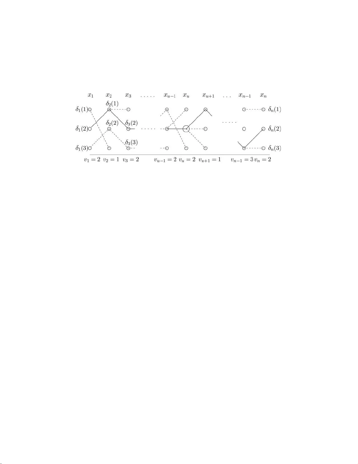
Bernoul li 14 (1), 2008, 180–206 DOI: 10.315 0/07-BEJ 105 The adjusted Viterbi training for hidden Mark o v mo dels J ¨ URI LEMBER 1 and ALEXEY K OLOYDENK O 2 1 T art u University, Liivi 2-50 7, T artu 50409 , Estonia. E-mail: jyril@ut.e e 2 Division of St atistics, University of Nott ingham, Nottingham NG7 2RD, UK. E-mail: alexey.koloydenko @nottingham.ac.uk The EM pr o c e dur e is a principal to ol for parameter estimation in the hidden Mark ov mo dels. How ever, applications replace EM by Viterbi extr action , or tr ai ning (VT). V T is computationally less intensiv e, more stable and has more of an in tu itiv e app eal, but VT estimati on is biased and does n ot satisfy the follo wing ﬁxe d p oint pr op erty . Hyp othetically , giv en an inﬁnitely large sample and initializ ed to th e true parameters, VT will generally mov e aw ay from the initial v alues. W e prop ose adjuste d Viterbi tr aining (V A), a new method to restore the ﬁxed p oin t prop erty and thus alleviate t he ov erall imprecision of the VT estimato rs, whil e preserving the computatio nal adv antages of the baseline VT algorithm. Simulations elsewhere ha ve shown th at V A appreciably impro ves th e precision of estimation in b oth th e sp ecial case of mixture mo dels and more general HMMs. H ow ever, being en tirely analytic, the V A correction relies on inﬁnite Viterbi alignments and associated limiting probability distributions. Wh ile explicit in the mixture case, the existence of these limiting measures is not ob v ious for more general HMMs. This p aper pro ves that under certain mild conditions, t h e required limiting d istri butions fo r general HMMs do exist. Keywor ds: Baum–W elc h; bias; computational eﬃciency; consis tency; EM; hidden Marko v models; maxim um likel ihoo d; parameter estimatio n; Viterbi extraction; Viterbi training 1. In tro duction Hidden Ma r k ov mo dels (HMMs) hav e b een called “ one of the most successful statistical mo delling ideas that ha ve [emerged] in the last forty years” [ 8 ]. Since their classica l application to digital comm unication in 1960s (see further references in [ 8 ]), HMMs ha ve had a deﬁning impact on the mainstream technologies of speech recognition [ 18 , 1 9 , 20 , 32 , 35 , 38 , 40 , 41 , 46 , 47 , 48 ] and, more recently , bioinformatics [ 11 , 12 , 25 ]. Natural language [ 21 , 36 ], imag e [ 30 ] and more g eneral spatial [ 17 ] mo dels are only a few of the n umerous other a pplications o f HMMs. Applications of HMMs inev ita bly face the problem of parameter estimation. Let us consider estimation of para meters of a ﬁnite-state hidden Mar k ov mo del (HMM) giv e n observ ations x 1: n = x 1 , . . . , x n on X 1: ∞ = X 1 , X 2 , . . . , the observ able pro cess of the HMM, This is an electronic reprint of the original article published by the ISI/BS in Bernoul l i , 2008, V ol. 14, No. 1, 180– 206 . This reprint diﬀers from the original in pagination and typographic detail. 1350-7265 c  2008 ISI/BS The adjuste d Viterbi tr aining for hid den Marko v mo dels 181 up to time n . F or any real application, X i can b e a ssumed to take on v alues in X = R D for some suitable D . Let Y 1: ∞ = Y 1 , Y 2 , . . . , the hidden la y er of the HMM, b e a (tim e- homogeneous) Marko v chain (MC) with state space S = { 1 , . . . , K } , tra nsition matrix P = ( p ij ) and initial distribution π = π P . T o every state l ∈ S , there c o rresp onds an emission distr ibution P l ( θ l ) with dens ity f l that is known up to the par ametrization f l ( x ; θ l ), θ l ∈ Θ l , where Θ l are ra ther general domains in R d . When Y k , k ≥ 1 , is in state l , an observ a tion x k on X k is emitted according to P l ( θ l ) a nd independent of ev er ything else. The Y 1: ∞ pro cess is also called a r e gime [ 31 ]. The maximum likeliho o d (ML) a p- proach has b ecome standard for estimation of ψ = ( P , θ ), the HMM parameters, where θ = ( θ 1 , θ 2 , . . . , θ K ). In part, this has b een due to the w ell-known theoretical prop erties of (lo cal) c onsistency a nd asymptotic normality generally enjoy ed by the ML estimators (MLE). Perhaps a mor e signiﬁcant reason for the widespread u se o f the ML approach has been the av ailability of the EM algorithm with its computationally eﬃcien t imple- men tation kno wn as the Baum–Welch o r simply Baum , o r forwar d–b ackwa r d algorithm [ 1 , 2 , 8 , 14 , 20 , 39 , 40 ]. Since EM can, in practice, b e slo w o r co mputationally exp ensiv e, it is commonly re- placed by V iterbi ext r action , or t r aining (VT), also known as the Baum–Viterbi algo- rithm. VT app ears to hav e b een in tro duced in [ 19 ] by F. J elinek and his colleagues at IBM in the con text o f spe e c h r ecognition, in which it has b een used extensiv ely e ver since [ 14 , 18 , 32 , 35 , 40 , 41 , 4 6 , 47 , 48 ]. Its computational stability (i.e., ra pid exit) and in tuitiv e app e a l [ 14 ] hav e also made VT p opular in natural language mo deling [ 36 ], im- age analysis [ 30 ] and bioinformatics [ 4 , 11 , 13 , 25 , 37 ]. VT is also related to constrained vector quan tization [ 10 ]. The main idea o f the metho d is to replace the computationa lly costly exp ectation (E-s tep) of the E M algorithm with an appropria te maximiza tion step that generally req uires less intensiv e computer op erations (otherwise, the t wo algorithms scale as K 2 n ). In sp eech recognition, e s sen tially the same training pro cedure was also describ ed b y L. Rabiner et al. in [ 22 , 41 ] (see a lso [ 39 , 40 ]) as a v aria tion o f the Lloyd al- gorithm used in v ector quantization. In that context, VT has gained the name se gmental K-me ans [ 14 , 22 ]. The analogy with vector quantization is esp ecially pro nounced when the underlying c ha in is triv ia lized to i.i.d. v aria bles, th us pro ducing a n i.i.d. sample from a mixture distribution. F or such mixture mo dels, VT was also describ ed b y R. Gray et al. in [ 10 ], where the training a lgorithm was consider ed in the vector quantization context under the name entr opy c onstr aine d ve ctor quantization (ECVQ) . A b etter-known name for VT in the mixture case is classiﬁc ation EM (CEM) [ 9 , 15 ], s tr essing tha t instead of the mixture likelihoo d, CE M maximizes the classiﬁc ation likel iho o d [ 4 , 9 , 15 , 33 ]. VT- CEM was also pa rticularly suitable for the ear ly eﬀo r ts in image segmen tation [ 44 , 4 5 ]. Also, for the uniform mixture of Gaussians with a common cov ariance matrix of the fo rm σ 2 I (where I is the K × K identit y matrix) and unknown σ , VT, or CEM, is equiv alent to the k- m e ans clus t ering [ 9 , 10 , 15 , 43 ]. 1.1. VT estimation and relev ance of V A to real applications The VT algorithm for estimation o f ψ can be describ ed as follows. Start with some initial v alues ψ (0) = ( P (0) , θ (0) ) a nd (use the Viterbi algorithm to) ﬁnd a realization of 182 J. L emb er and A. Koloydenko Y 1: n that maximizes the lik eliho o d of the given observ a tions. An y suc h n -tuple of states is called a Viterbi , or for c e d, alignment . An alignment partitions the orig inal sample x 1: n in to subsamples corresp onding to distinct states. If reg arded as an i.i.d. sample from P l ( θ l ), the subsample corres ponding to state l gives rise to ˆ µ n l , the maximum likelihoo d estimate (MLE) of θ l , l ∈ S . At step m + 1 , these estimates replace θ ( m ) . The transition probabilities are s imilarly estimated (by MLE) from the curr en t alignment . The up dated parameters ψ ( m +1) are s ubse quen tly used to obta in a new alignmen t, and so on. It can be sho wn that, in gener al, ψ ( m ) conv erg es (to some ψ ∗ ( x 1: n , ψ (0) )) in ﬁnitely man y steps m [ 22 ]; also, it is usually m uch faster than the Baum algorithm. Note that when each f l is modelled a s a mixture, which is common in audio and visual processing , VT can be applied at b oth stages of this mo del – ﬁrs t, in its genera l form (i.e., as with f l general) a nd then in its CEM fo r m to learn each individual f l . Alternatively , the orig inal HMM ca n, from the very b eginning, be replaced b y the equiv alent o ne with hidden states ( l , s ( l )), where s ( l ) indicates the (sub)component of f l . VT can then also be applied to this new HMM as, for exa mple, has b een done in the Philips sp eec h recognition sys tem [ 35 ]. Despite its attractiveness, VT can be challenged, a s its estimator s are gener a lly biased and not consisten t. This has been noted, at leas t in the case of mixtures, since [ 4 ], with a sp eciﬁc caveat issued in [ 49 ]. Sim ula tions in [ 27 ] and [ 24 ] illustrate apprecia ble biases in VT estimation in the i.i.d. and more general HMM settings, resp ectively . A t the same time, these facts are not surprising. Indeed, unlik e EM, whic h increases the likelihoo d of ψ giv en x 1: n , VT increases the join t likelihoo d of the (hidden) state sequence y 1: n and the pa rameters ψ , g iv en x 1: n . According to [ 34 ], under certain conditions, the diﬀerence betw een the t wo o b jectiv e functions v anishes as D , the dimension o f the emission X i , grows suﬃciently large relative to log( K ), whic h can b e r e alistic in isolate d wor d r e c o gni- tion [ 34 ]. How ever, as later clariﬁed in [ 14 ], this do es not imply closeness o f the parameter estimates obtained by EM and VT (unless the algorithms are initialized identically) since bo th p erform a loca l, rather than global, optimization. Certainly , unbiasedness a nd consistency a re neither necessar y nor suﬃcien t for a pro- cedure to perform w ell in applications [ 45 ]. How ever, there are indications that some applications, such as se gment-b ase d sp e e ch r e c o gnition [ 46 ], do prefer the standar d, that is, EM- t yp e, likelihoo d maximization. Also , [ 46 ] notes that c onventional sp e e ch r e c o gniz- ers would prefer the ‘smoo ther conv erge nce ’ of ψ ( m ) under EM, presuma bly over the more a brupt, greedy convergence of ψ ( m ) under VT. A t the same time, it app ears that in complex en vir onmen ts, VT can be appreciably simpler to implemen t than EM [ 46 ]. Hence, it appear s to b e sensible to combine the simplicity of VT’s implementation with the desirable pr operties of EM. Indeed, there are v ar iations of VT that use mo r e than one bes t a lignmen t or several per turbations of the b est a lig nmen t [ 36 ]. V A, our type of adjusted VT, is of a diﬀerent nature as it improv es the estimation precision b y means of analytic calculations and do es not compute more than one optimal alignmen t per iteration. Moreov er, w e suggest that in vestigating suc h alternatives to VT and E M for real applications is now adays m uch more appealing than ev er befor e, thanks to the abundance of vir tually inﬁnite and freely av a ilable streams of a udio and video (e.g., r e a l-time broadcasting) as w ell as biological data. Actually , practitioners hav e already realized this by shifting from entirely The adjuste d Viterbi tr aining for hid den Marko v mo dels 183 supe r vised to semi- and unsup ervised modes of training [ 50 ]. One na ¨ ıve realization of these ideas is to simply use the estimates obtained from a lab eled s ample (i.e., with y 1: n known) as the initial guess ψ (0) for a further unsupe r vised retraining. A mo re dedicated application w ould be mo del adaptation , wherein the mo del ψ (0) (initially trained in any mo de) may need to be adapted to a new environmen t (e.g., spea k er ) diﬀering fro m the original one mos tly , or only , b y the emission parameters. Applicabilit y of our adjusted VT for mixture mo dels and situations when the transition probabilities ar e either known or nuisance is further discussed in Section 2.3 . Finally , simulations in [ 27 ] a nd [ 24 ] clea rly show that V A, our metho d of adjusting VT, does signiﬁcantly impro ve the precision o f VT estimation. In those experiments, the V A e s timates ar e always compara ble to the E M estimates, while the V A algorithm is only margina lly mor e in tensive than the baseline VT algorithm. 1.2. The adjusted Viterbi tr ain ing a nd c ontribution of t his w ork Is it p ossible to adjust VT in an analytic w ay in order to enjoy b o th the desirable prop- erties of VT (f ast c on vergence of ψ ( m ) , ov er all computational feasibilit y , simplicity of implemen tation and an ov erall in tuitive app eal) a nd more consistent estimation? En- suring that an algorithm ha s the true p ar ameters as its asymptotic al ly ﬁxe d p oint turns out to b e piv otal in constructing such adjusted estimators. Eviden tly , this ﬁxed p oint prop ert y holds for EM, but not for VT. Namely , for a suﬃcien tly large sample, the EM algorithm ‘r ecognizes’ and ‘conﬁrms’ the true par ameters. In cont rast to this, an itera- tion of VT generally disturbs the correc t v alues noticeably . In [ 27 ], w e hav e prop osed to mo dify VT in or der to make the true par a meters an asymptotically ﬁxed p oin t o f V A, the resulting algorithm. In or der to understand V A, it is crucial to understand the as ympt otic b ehaviors of ˆ µ n l and ˆ p n ij , the maximum likeliho od estimators based on the Viterbi alignment. Since the alignment depends on ψ (0) , the initial v alues of the par ameters (and on the tie-breaking rule, which is ignor e d for the time b eing), so do ˆ µ n l ( ψ (0) , X 1: n ) and ˆ p n ij ( ψ (0) , X 1: n ). Note that, for ψ to b e asymptotically ﬁxed by an estimation algor ithm, it means that if ψ = ( P , θ ) are the true par a meters and are used to compute the alignment, then ˆ µ n l ( ψ , X 1: n ) − → n →∞ θ l a.s. ∀ l ∈ S ; ˆ p n ij ( ψ , X 1: n ) − → n →∞ p ij a.s. ∀ ( i, j ) ∈ S 2 . (1.1) The reason why VT does not enjo y th e desir ed ﬁxed point property is that ( 1.1 ) need not ho ld in g eneral [ 4 , 49 ]. Hence, in order to restor e the ab ov e ﬁxed p oin t pro perty in VT, we need to v er ify that the sequences in ( 1.1 ) converge almo st surely and, provided they do, exhibit their limits. This pap er essen tially accomplishes these tasks. Namely , we show that (under certain mild conditions) the e mpirical measur es ˆ P n l ( ψ , X 1: n ) ob- tained via the Viterbi alignmen t do con verge w eakly to a cer tain limiting probabilit y measure Q l ( ψ ) ( 2.5 ) a nd that, in general, Q l ( ψ ) 6 = P l ( θ l ). In [ 24 ], we have s hown that under general conditions on the densities f l ( x ; θ l ) (and, for Θ l , closed subsets of R d ), the 184 J. L emb er and A. Koloydenko ab o ve con v ergence ˆ P n l ( ψ , X 1: n ) ⇒ n →∞ Q l ( ψ ) a.s. (properly int ro duced in ( 2.5 )) implies conv erg ence of ˆ µ n l , that is, ˆ µ n l ( ψ , X 1: n ) − → n →∞ µ l ( ψ ) a.s., where µ l ( ψ ) def = arg max θ ′ l ∈ Θ l Z ln f l ( x ; θ ′ l ) Q l (d x ; ψ ) . (1.2) Since, in general, Q l ( ψ ) 6 = P l ( θ l ), clea rly µ l ( ψ ) need not equal arg max θ ′ l R ln f l ( x ; θ ′ l ) × P l (d x ; θ l ). In order to obtain the above results, in Section 4 , w e extend Viterbi alignmen ts, or paths, ad inﬁnitum. Namely , considering (ﬁnite) Viterbi alignments with tie-brea king rules of a sp ecial kind, we prove the exis tence of a decoding v : X ∞ → S ∞ such that, for almost every realization x 1: ∞ , the f ollowing property holds: for every m ∈ N , there exists a n n = n ( x 1: ∞ , m ) ∈ N , n > m , s uc h that the co deword v ( x 1: ∞ ) and the Vit erbi alignment based on x 1: n agree up to time m . T o emphasize the dependence of v on ψ , we will write v ( x 1: ∞ ; ψ ). It can then also b e shown that when ψ are the true parameters, the proces s V def = v ( X 1: n ; ψ ) is r egenerative. In particular, for any i , j ∈ S, there exists q ij ( ψ ) ≥ 0 suc h that P j q ij ( ψ ) = 1 for every i ∈ S and ˆ p n ij ( ψ ; X 1: n ) a . s . − → n →∞ q ij ( ψ ) . (1.3) Again, in general, p ij 6 = q ij ( ψ ). Reduction of the biases µ l ( ψ ) − θ l and q ij ( ψ ) − p ij is the main feature of the adjusted Viterbi training. 1.3. Previous r elated w ork W e are not aw a r e of any sys tematic tr e a tmen t of asymptotic reduction of the bias in VT estimation (without compromising the adv antages of the VT algorithm over Baum– W elch) preceding [ 27 ]. In [ 23 ], how ever, a sequential version o f VT (‘the segmen ta l K- means algor ithm’) is sugges ted, which can allegedly reduce the estimation bias asymptot- ically . The suggested mo diﬁca tion a ppears substantially diﬀerent from our adjustmen t, although we ha ve b een unable to ev aluate the algo r ithm of [ 23 ] thoro ughly due to the lack of detail in its descr iption in [ 23 ] or anywhere else to date. Moreov er, to the b est of our knowledge, there has be e n no systematic study of asymp- totic prop erties of the Viterbi alignments to date b esides certain attempts made by Kogan in [ 23 ] in the con text o f the sequential v ersion of VT (see ab ov e) and, more recentl y , by Calieb e and R¨ osler in [ 7 ] a nd Calieb e in [ 5 ]. Both gro ups ha ve g iv en thorough treatments of certain s pecial cases, mostly K = 2, but this, as w e explain below, is to o sp ecial. Impo rtan tly , it was recognized in [ 23 ] that under certain conditions, longer Viterbi alignments can be obtained piecewise. Roug hly , the end-p oints of the pieces and the (random) times o f their occur rence were termed ‘special columns’ and ‘most informa tiv e stopping times’, resp ectiv ely . In [ 5 , 7 ], related notions of ‘meeting states’ and ‘meeting times’ are used. Independently of [ 5 , 7 , 23 ], we hav e built our theory on the notion of no des (roughly , observ ations emitted from the ‘special columns’; see Section 3.1 ) and the The adjuste d Viterbi tr aining for hid den Marko v mo dels 185 stopping times of their o ccurrence. If deﬁned to b e indep enden t of a particular global tie-breaking rule, the meeting times of [ 5 ] w o uld corresp ond to ‘strong no des’ of order 0, a particular type of nodes. More impo rtan tly , ev en o ur (general) no des, which are essentially equiv alen t to the sp ecial columns of [ 23 ] and ‘path cross ing s’ o f [ 5 , 7 ], are not suﬃciently gener al in the sense that HMMs with ap erio dic a nd irreducible Markov chains need not necessarily have specia l columns, or no des, inﬁnitely often almost surely, despite the claim to the contrary made in Theorem 2 of [ 23 ] (stated without pro of a nd implicitly cited in [ 14 ]). F or a counterexample, w e refer to E xample 3 .11 in [ 26 ], a downloadable preprint of this pap er. Appropr iate s uﬃcien t conditions to guar an tee the desired prop ert y hav e also b een given in [ 26 ] for the ﬁrst time. Implicitly , the alignmen t pro cess in [ 23 ] was r ecognized as regenerative with resp ect to the ‘most informative stopping times’. The limiting alignment proces s of [ 5 ] is alrea dy explicitly shown to b e reg enerativ e. Regenerativity with resp ect to (the times of ) no des is also essential for our purpose of exhibiting the limiting measur es Q l ( ψ ) ( 2.5 ) and q ij ( ψ ) ( 1.3 ). Conv erg ence of the Viterbi paths w as , to the b est of o ur knowl edge, ﬁrst ser iously considered in [ 5 , 7 ], where the existence of inﬁnite a lignmen ts for certain special cases, such as K = 2 and some HMMs with additiv e white Gaussian noise, was also prov en. While innov a tiv e, the main r e s ult of [ 7 ] (Theorem 2) makes several restrictive ass umptions preven ting its ex tension b ey ond the K = 2 case. As its by-pro duct, this work extends some, and cor rects other, results of [ 5 , 7 ]. This is explained in detail in the appropriate paragr aphs of Sections 3.1 – 3.3 and Section 4 . Also, note that our g oal of exhibiting Q l ( ψ ) and q ij ( ψ ) extends b ey o nd solely deﬁni ng inﬁnite Viterbi alignmen ts (the main goal of [ 7 ]). 1.4. Organization of the rest of the paper First, in Section 2 , we pro perly in tro duce the ba seline a nd adjusted Viterbi training pro- cedures (Section 2 .2 ) for HMMs. In Section 2.3 , the adjusted Viterbi training is discussed in the context of the following tw o imp ortant v ariations on the main situation: the regime parameters are known or nuisance. Mo re g eneral is sues of implementation are discussed in Section 2.4 . Sections 2.3 and 2 .4 can be skipp ed without interruption of th e main presentation. Recall that our ultimate goal has b een asymptotic reduction of the bias in VT estima- tion for a s genera l a class of HMMs as pos s ible. The main goal of this paper , howev er, is to prov e the existence of the limiting measures Q l ( ψ ) ( 2.5 ) and q ij ( ψ ) ( 1.3 ) that un- derpin our a pproach to achieving the ultimate goa l. A signiﬁcan t eﬀort has been made to achiev e this accurately and under as non-restrictive conditions as p ossible. This is the main reas o n why we ca nnot directly reuse the to ols us e d by o thers ([ 5 , 7 , 23 ]). As w e reit- erate further in Section 3 , the asymptotic b ehavior o f the Viterbi alignment is not trivial and do es require sp e c ial to ols. Th us, no des and b arriers , our main to ols, are presen ted in Sections 3.1 and 3.3 , respe ctiv ely . In Sectio n 3.2 , we explain o ur piecewise construction of the pr op er Viterbi alignments. This is s till at the level of individual rea lizations of the HMM pro cess. In Section 3.3 , barriers, on the other hand, extend our construction for 186 J. L emb er and A. Koloydenko almost ev ery realization o f the HMM pro cess. This is the essence of Lemmas 3.1 and 3.2 , the ﬁrst of the t wo main re s ults of this paper. In Section 4 , we deﬁne V 1: ∞ , the pr op er inﬁnite alignment pr o c ess . Fina lly , in the s ame section w e prov e the existence o f the mea- sures Q l ( ψ ) and q ij ( ψ ), our second main result, using r e g enerativit y of the aug mented pro cess ( V 1: ∞ , X 1: ∞ ) (Theorem 4.1 and Corollar y 4.1 ). Exhibiting the measures Q l ( ψ ) under v er y general conditions has nece s sitated several rather technical constructions, mainly used to prov e Lemmas 3.1 and 3 .2 . Due to spatial limitations, they a re no t given her e, but rather app ear in [ 26 ]. 2. The adjusted V ite rbi training 2.1. The mo del Recall that Y 1: ∞ takes v alues in S = { 1 , . . . , K } and has transition matrix P . Let Y 1: ∞ be irreducible and aper iodic, hence a unique π = π P exists. Let the emission distrib utions P l ( θ l ), l ∈ S , be deﬁned on ( X , B ), where X a nd B are a separable metric space and the corresp onding Borel σ -algebra, resp ectiv ely . Let f l be the densit y of P l ( θ l ) with resp ect to a s uitable r eference meas ure λ o n ( X , B ). Deﬁnition 2.1. The sto chastic pr o c ess X is a hidden Markov mo del if ther e is a (me a- sur able) function h such that, for e ach n , X n = h ( Y n , e n ) , wh er e e 1 , e 2 , . . . ar e i. i.d. and indep endent of Y . (2.1) Hence, the emission distribution P l ( θ l ) is the distribution o f h ( l , e n ). The distribution of X is completely determined b y the regime para meters P and the emission distributions P l ( θ l ), l ∈ S . The proces s X is also α - mixing and, therefor e, erg odic [ 14 , 16 , 29 ]. 2.2. Viterbi alignmen t and training Let Λ( y 1: n ; x 1: n , ψ ) = P ( Y 1: n = y 1: n ) n Y i =1 f y i ( x i ; θ y i ) , where P ( Y 1: n = y 1: n ) = π y 1 n Y i =2 p y i − 1 y i , be the lik eliho o d functions of the y 1: n , treated as parameter s . Given x 1: n , let V ( x 1: n ; ψ ) be the set o f all maxim um-likeliho o d estimates of y 1: n . These estimates, or paths, ar e eﬃcient ly obtained b y the Viterbi algorithm and are called the Viterbi alignments . The non-uniqueness of the alignmen ts causes substantial technical incon veniences. In Section 3.2 , we specify unique v ( x 1: n ; ψ ) ∈ V ( x 1: n ; ψ ) for every n ∈ N and x 1: n ∈ X n (and every ψ ) in a consistent manner that is suitable to prov e the existence o f Q l ( ψ ). Meanwhile, the uniqueness o f v ( x 1: n ; ψ ) is an assumption. VT estimation of ψ is deﬁned formally as follows (where I A is the indicator function o f set A ): The adjuste d Viterbi tr aining for hid den Marko v mo dels 187 (1) choo se initial v alues for the parameters ψ ( k ) = ( P ( k ) , θ ( k ) ), k = 0 ; (2) given ψ ( k ) , curren t parameters, o bta in the alignment v ( k ) = v ( x 1: n ; ψ ( k ) ); (3) up date the regime parameters P ( k +1) def = ( ˆ p n ij ) as given b y ˆ p n ij def =      P n − 1 m =1 I { i } ( v ( k ) m ) I { j } ( v ( k ) m +1 ) P n − 1 m =1 I { i } ( v ( k ) m ) , if n − 1 X m =1 I { i } ( v ( k ) m ) > 0 , P ( k ) ij , otherwise, i, j ∈ S ; (2.2) (4) as s ign x m , m = 1 , 2 , . . . , n , to class v ( k ) m and, equiv alently , deﬁne empirica l measures ˆ P n l ( A ; ψ ( k ) , x 1: n ) def = P n m =1 I A ×{ l } ( x m , v ( k ) m ) P n m =1 I { l } ( v ( k ) m ) , A ∈ B , l ∈ S ; (2.3) (5) for each cla ss l ∈ S , obtain ˆ µ n l ( ψ ( k ) , x 1: n ), MLE of θ l , given by ˆ µ n l ( ψ , x 1: n ) def = arg max θ ′ l ∈ Θ l Z ln f l ( x ; θ ′ l ) ˆ P n l (d x ; ψ, x 1: n ) (2.4) and for all l ∈ S , let θ ( k +1) l def =      ˆ µ n l ( ψ ( k ) , x 1: n ) , if K X m =1 I { l } ( v ( x 1: n ; ψ ( k ) ) m ) > 0, θ ( k ) l , otherwise. T o b etter interpret VT, suppo s e that, at some step k , ψ ( k ) = ψ , th us v ( k ) is obtained using the true par ameters. Let y 1: n be the actual hidden realization of Y 1: n . The training ‘pretends’ that the a lignmen t v ( k ) is p erfect, that is, that v ( k ) = y 1: n . If the a lig nmen t were indeed perfect, then the empirical measures ˆ P n l , l ∈ S , would b e obtained fro m the i.i.d. samples gener a ted from P l ( θ l ) a nd the MLE ˆ µ n l ( ψ , X 1: n ) would b e natura l estimators to use. Under these assumptions, ˆ P n l ( ψ , X 1: n ) ⇒ P l ( θ l ) a s n → ∞ a.s. and, pro vided that { f l ( · ; θ l ) : θ l ∈ Θ l } is a P l -Glivenk o– C a n telli class and Θ l is equipp ed with a suitable metric, we would have lim n →∞ ˆ µ n l ( ψ , X 1: n ) = θ l a.s. Hence, if n is suﬃcien tly large, then ˆ P n l ( ψ , X 1: n ) ≈ P l ( θ l ) and θ ( k +1) l = ˆ µ n l ( ψ , x 1: n ) ≈ θ l = θ ( k ) l for every l ∈ S . Similar ly , if the alignment is per fect, then lim n →∞ ˆ p n ij ( ψ , X 1: n ) = P ( Y 2 = j | Y 1 = i ) = p ij , a.s . Th us, for the per fect alignment, ψ ( k +1) = ( P ( k +1) , θ ( k +1) ) ≈ ( P ( k ) , θ ( k ) ) = ψ ( k ) = ψ , that is, ψ w ould be (approximately) a ﬁxed point of the training algor ithm. Certainly , the alignmen t, in general, is not p erfect, even when it is co mputed with the true parameters. In particular , the e mpir ic a l measur es ˆ P n l ( ψ , X 1: n ) can be rather far from those based on i.i.d. samples from P l ( θ l ). Hence, we hav e no rea son to expect that lim n →∞ ˆ µ n l ( ψ , X 1: n ) = θ l a.s. and lim n →∞ ˆ p n ij ( ψ , X 1: n ) = p ij a.s. Moreover, we do not even kno w wheth er the sequences of empirica l measures ˆ P n l ( ψ , X 1: n ), or MLE estimators ˆ µ n l ( ψ , X 1: n ) and ˆ p n ij ( ψ , X 1: n ), conv erg e almost surely at all. 188 J. L emb er and A. Koloydenko As stated in Theorem 4.1 , under certain mild conditions, there exist pr obabilit y mea- sures Q l ( ψ ), l ∈ S , such that ˆ P n l ( ψ , X 1: n ) = ⇒ n →∞ Q l ( ψ ) a.s. (2.5) F ro m the pro of of Theorem 4.1 , it also follows (Corollary 4.1 ) that for every i ∈ S , there exist probabilities q i 1 , . . . , q iK such that ( 1.3 ) holds. In general, µ l ( ψ ) 6 = θ l and q ij ( ψ ) 6 = p ij . In o rder to reduce the biases θ l − µ l ( ψ ) and p ij − q ij ( ψ ), w e ha v e pr o posed the adj uste d Viterbi t ra ining . Na mely , suppos e that ( 1.2 ) and ( 1.3 ) hold and consider the mappings ψ 7→ µ l ( ψ ) , ψ 7→ q ij ( ψ ) , l, i, j = 1 , . . . , K. (2.6) The functions in ( 2.6 ) do not depend on x 1: n , hence the following corrections are w ell deﬁned: ∆ l ( ψ ) def = θ l − µ l ( ψ ) , R ij ( ψ ) def = p ij − q ij ( ψ ) , l , i, j = 1 , . . . , K. (2.7) Based on ( 2.7 ), the adjuste d Viterbi tr aining re pla ces VT steps (3) a nd (5) as given below: (3) for every i, j ∈ S , upda te the matrix P ( k +1) def = ( p ( k +1) ij ) accor ding to p ( k +1) ij def = ˆ p n ij + R ij ( ψ ( k ) ); (2.8) (5) for all l ∈ S , let θ ( k +1) l def = ∆ l ( ψ ( k ) ) +      ˆ µ n l ( ψ ( k ) , x 1: n ) , if K X m =1 I { l } ( v m ) > 0 , θ ( k ) l , otherwise. Provided n is suﬃciently lar ge, V A, as desired, has the true par a meters ψ as its (ap- proximately) ﬁxed p oin t. Indeed, supp ose that ψ ( k ) = ψ . F rom ( 1.2 ), ˆ µ n l ( ψ ( k ) , x 1: n ) = ˆ µ n l ( ψ , x 1: n ) ≈ µ l ( ψ ) = µ l ( ψ ( k ) ) for all l ∈ S . Similarly , fro m ( 1.3 ), ˆ p n ij ( ψ ( k ) , x 1: n ) = ˆ p n ij ( ψ , x 1: n ) ≈ q ij ( ψ ) = q ij ( ψ ( k ) ) for all i, j ∈ S . Thus, θ ( k +1) l = ˆ µ n l ( ψ , x 1: n ) + ∆ l ( ψ ) ≈ µ l ( ψ ) + ∆ l ( ψ ) = θ l = θ ( k ) , l ∈ S, (2.9) p ( k +1) ij = ˆ p n ij ( ψ , x 1: n ) + R ij ( ψ ) ≈ q ij ( ψ ) + R ij ( ψ ) = p ij = p ( k ) ij , i, j ∈ S. (2.10) Hence, ψ ( k +1) = ( P ( k +1) , θ ( k +1) ) ≈ ( P ( k ) , θ ( k ) ) = ψ ( k ) . Example 1 (Mixtur es). Let X 1 , X 2 , . . . b e i.i.d. a nd follow a mixture distribution with densit y P K l =1 π l f l ( x ; θ l ) a nd (positive) mixing weigh ts π l . Such a sequence is an HMM with transition probabilities p ij = π j for all i, j ∈ S . In this specia l case, the a lignmen t The adjuste d Viterbi tr aining for hid den Marko v mo dels 189 and the measures Q l are eas y to exhibit. Indeed, for any set of para meters ψ = ( π, θ ), the alignmen t v ( x 1: n ; ψ ) can b e obtained v ia a generalized V or onoi p artition S ( ψ ) = { S 1 ( ψ ) , . . . , S K ( ψ ) } , where S 1 ( ψ ) = { x ∈ X : π 1 f 1 ( x ; θ 1 ) ≥ π j f j ( x ; θ j ) , ∀ j ∈ S } , (2.11) S l ( ψ ) = { x ∈ X : π l f l ( x ; θ l ) ≥ π j f j ( x ; θ j ) , ∀ j ∈ S }\ l − 1 [ k =1 S k ( ψ ) , l = 2 , . . . , K. (2.12) Now, the alignment ca n be deﬁned p oin twi se as follows: v ( x 1: n ; ψ ) = ( v ( x 1 ; ψ ), . . . , v ( x n ; ψ )), where v ( x ; ψ ) = P K k =1 k I S k ( ψ ) ( x ), which returns l if and only if x ∈ S l ( ψ ). The conv ergence ( 2.5 ) no w follo ws immediately from the strong law of larg e n umbers. Indeed, if ψ are the true parameters and if the alignment is obtained based on ψ , then the SLL N immediately gives ˆ P n l ( ψ ) ⇒ Q l ( ψ ) almost surely , with densities q l ( x ; ψ ) of Q l ( ψ ) ∝ f ( x ; ψ ) I S l ( ψ ) = ( P K k =1 π k f k ( x ; θ k )) I S l ( ψ ) , l = 1 , 2 , . . . , K. Hence, the limit of the class-conditiona l MLE ˆ µ n l is giv en b y µ l ( ψ ) = a rg max θ ′ l ∈ Θ l Z S l ( ψ ) ln f l ( x ; θ ′ l ) K X k =1 π k f k ( x ; θ k ) ! λ (d x ) , (2.13) which , dep ending on the mo del, can diﬀer from θ l signiﬁcantly ([ 24 , 27 ]). Also, ( 1.3 ) follows easily in this case (see [ 27 ] for further details). Namely , note that ˆ π n l ( ψ , X 1: n ) a . s . − → n →∞ q l ( ψ ) = K X k =1 π k Z S l ( ψ ) f k ( x ; θ k ) λ (d x ) . (2.14) Thu s, in the sp ecial case of mixtures, the adjustmen ts ∆ l and R l are r elativ e ly easy to obtain and the adjusted Viterbi t raining is e a sy to implemen t. The sim ula tions in [ 27 ] hav e lar g ely supported the theory , demonstrating b oth the computational adv antage of V A o ver EM and the increased precision of V A relative to VT. 2.3. V A for ‘independen t t r ain ing’ Some a pplications, suc h as lar ge vocabulary sp eech recog nition systems [ 35 ], ﬁx the regime para meters exogenously . With the appropriate simpliﬁcations, th e baseline and adjusted Viterbi training pro cedures, as well as the E M alg orithm, immediately apply in such situations. In fact, in [ 24 , 2 7 ], V A is discussed pr imarily in this simpliﬁed cont ext. It ca n then b e arg ued tha t, when the regime par a meters a re known, V A is unnecessar y as MLI , the maximum likelihoo d estimation under the indepe ndence assumption (whic h can also b e called indep endent t r aining ), applies. L et us discuss this issue in more detail. According to [ 31 ], MLI estimates the emission parameters (and possibly π when P is unknown and not of interest) o f general (erg odic) HMMs pretending that Y 1 , Y 2 , . . . , ar e independent, that is , the entire HMM follo ws a mixture mo del. This is app ealing since 190 J. L emb er and A. Koloydenko the marg inal distribution o f the emissio ns of a n y HMM (with a stationar y regime) is in- deed the mixture with density P k π k f k ( · ; θ k ). Thus, MLI is an instance of the maximu m pseudo-likeli ho o d (MPL) based on the ab ov e mixture appr o x imation. The MLI– MPL es - timators for the emission parameters are (lo cally) consistent [ 31 , 42 ] and c a n also be delivered by EM (for mixtures ). Similarly to the genera l ca se, when computational re- sources do matter, VT (for mixtures) can also be used instead o f EM in this ca se. As in the general cas e, Baum–W elc h and VT scale identically , but their co mmon computational complexity is now K n , as oppo sed to K 2 n . The compar ativ e computational p erformances of Ba um– W elch and VT for mixtures and in the general ca se are also similar (the Baum algorithm involv es more in tensive o perations). A t the sa me time, as Example 1 in Sec- tion 2.2 ab o ve shows, the VT estimators are still not consistent and, in particular, the correction ∆ l = θ l − µ l ( ψ ), with µ l ( ψ ) as in ( 2.13 ), ca n b e signiﬁcant. Let us ma k e ano ther p oint. L e t θ be ﬁxed and let ∆ l and ∆ ∗ l be the co rrections obtained with and without the independence a ssumption ( p ij = π j , i, j ∈ S ), resp e c tively . The following intuitiv e fact has b een shown in [ 24 ] by sim ulation: ∆ ∗ l ≤ ∆ l and the diﬀerence ∆ l − ∆ ∗ l widens as the dep endence in P beco mes stronger. This suggests that there is more to gain b y adjusting VT for mixtures tow ar d MPL-MLI than b y adjusting VT fo r the actual HMM tow ar d the true MLE. Th us, if one is in teres ted in a co mputationally eﬃcient approximation to (the Ba um implementation o f ) MPL–MLI, the adjusted Viterbi training for mixtures is a sensible alternative to the baseline Viterbi training for mixtures. Also, note that V A for mixture models was studied in [ 27 ], where, in addition to the theoretical demonstration of the VT bias, it was also shown by simulations that this bias could be signiﬁc antly reduced b y V A. Impo rtan tly , in the mixture case, the V A corr ections are often g iv en explicitly , which s impliﬁes the implementation o f the algor ithm. The independent training a pproach is a lso a natural choice when the underlying regime is a gener al ergo dic pro cess (not necessar ily Marko v) with an (unknown) stationary distribution π . Even when not of direct in ter e st, π can a nd needs to b e es timated. Again, if computational eﬃciency is an issue, V A for mixtures with unknown weigh ts is an alternative to the Baum algorithm (for mixtures with unkno wn w eights). Note that in this case, the co r rections R l = π l − q l ( ψ ), with q l ( ψ ) as in ( 2.14 ), should be used in addition to the ∆ l corrections. Simu lations in [ 27 ] sho wed a clear adv a n tag e of using bo th adjustments R l and ∆ l for mixture models with unknown π . In particular, V A was, as usual, both supe r ior to VT and only slightl y inferior to E M, in precision. Remark ably , taking few steps to sta bilize, V A also o utperformed VT in total run time. 2.4. Implemen tation T o implemen t V A in pr a ctice, explicit expres sions for Q l ( ψ ) (or µ l ( ψ )) a nd q ij ( ψ ) are desirable. In general, ho wev er, these functions ca n b e v ery diﬃcult to compute with high precision. A t the same time, as w a s just p oin ted out in Section 2.3 ab o ve, the co rrections ∆ l and R l are easy to obtain for a broad class of mixture models including the mo st commonly used mixtures of Gaussians with equal and known cov ariances. Other deta ils of V A implementation ha ve been addres sed in [ 27 ] and [ 24 ] for mixture and mor e genera l The adjuste d Viterbi tr aining for hid den Marko v mo dels 191 mo dels, respectively . F o r one example, [ 24 ] discusses the sto chastic al ly adj uste d Viterbi tr aining , an eﬃcien t implementation of V A for general HMMs when the co rrections can- not b e obtained analytically . Although sim ulatio ns do require extra computations, the ov era ll complexity of the sto c hastically adjusted VT can still b e considera bly lower than that of Baum–W elch. Certainly , this requires further in vestigation. Other pr actical issues are also a sub ject of con tin uing in vestigation. 3. Inﬁnite Viterbi alignmen t The idea of the adjusted Viterbi training is based o n, ﬁrstly , the o bserv ation that the maximum likelihoo d path (the Viterbi alig nmen t) diﬀers substantially from the underly- ing Mar k ov chain and, secondly , that these diﬀerences need to b e acco un ted for in o rder for the ov er all HMM-based inference to be accurate. Our adjusted Viterbi training need not b e the only metho d to co r rect the training pro cess fo r these diﬀerences. How ever, any such metho d must inevitably apprecia te the asymptotic proper ties o f both th e Viterbi alignment and the subsamples of the emissions as classiﬁed by the alignment. After all, it is these features that determine the pr operties of the VT estimators in genera l and the asymptotic bias of VT in particular. Even disreg arding the non-uniqueness o f the Viterbi a lignmen t v ( x 1: n ) (dependence on ψ is temp orarily s uppressed), the asymptotic b ehavior of v ( X 1: n ) is no t trivial since the ( n + 1 )th o bserv ation can in principle ch ange the entire alignment bas e d o n x 1: n . Namely , let v ( x 1: n ) and v ( x 1: n +1 ) be the alignments based on x 1: n and x 1: n +1 , respec tiv ely . It might happen with p ositiv e probability that v ( x 1: n ) i 6 = v ( x 1: n +1 ) i for every i = 1 , . . . , n . A t the same time, the fact that the alignment ch anges inﬁnitely often makes it diﬃcult to deﬁne a meaningful inﬁnite alignmen t pr ocess . F or most HMM s, howev er, there is a po sitiv e proba bility of observing x 1: n such that, regardless of the v alue of the ( n + 1)th o bs e r v ation (provided n is suﬃciently lar ge), the alignments v ( x 1: n ) and v ( x 1: n +1 ) agree fo r a suﬃcien tly long time u ≤ n . Consequently , reg a rdless of wha t happens in the future, the ﬁrst u elemen ts of the alignment remain constant. Pr o vided that there is an increasing unbounded sequence u i ( u < u 1 < u 2 < · · · ) such that the alignment up to u i remains constant , inﬁnite alignments can then b e deﬁned. The observ ation that for most commonly used HMMs, a t ypica l realizatio n x 1: ∞ has inﬁnitely many u i is the basis of our further analysis. Consider the follo wing simple mo del that g ua ran tees almo st every x 1: ∞ to ha ve in- ﬁnitely ma n y u i ’s and provides an insight into a signiﬁcant ly mor e general scenario. Let state 1 ∈ S and ev ent A ∈ B be suc h that P 1 ( A ) > 0, while P l ( A ) = 0 for l = 2 , . . . , K . Thu s, any obs erv ation x u ∈ A is almost surely g e ner ated under Y u = 1 and we say that x u indic ates its state . Consider n to b e the ter minal time and note tha t any p ositive like- liho od pa th, including v ( x 1: n ), the maxim um likelihoo d one, must go through the state 1 at time u . This allows us to split the Viterbi alignmen t into v 1 and v 2 , an alignment from time 1 thro ugh time u a nd an alignmen t from time u throug h time n , r e s pectively . Namely , v 1 and v 2 maximize Λ( y 1: u ; x 1: u ) and Λ( y u : n ; x u : n ), the respective lik eliho o ds. By concatenating v 1 with v 2 2: n − u +1 (removing the ov erlapping v 2 1 = 1 ), we obtain v ( x 1: n ) 192 J. L emb er and A. Koloydenko that maximizes Λ( y 1: n ; x 1: n ). Clearly , a n y additional observ ations x n +1: m do not change the fact th at x u indicates its state. Hence, for any extension o f x 1: n , the ﬁrst pa rt of the alig nmen t is alwa y s v 1 . Thus, any obser v a tion that indicates its state also ﬁxes the beg inning of the a lignmen t. Since o ur HMM is a stationar y pro cess that has a p osi- tiv e pro babilit y o f generating state-indicating observ ations, there will be inﬁnitely many such observ a tio ns almost surely. (The ov erla p v 2 1 = 1 is sur ely a nuisance since v 2 2: n − u +1 maximizes Λ( y u +1: n ; x u +1: n ) with the initial distribution π r eplaced by ( p 1 j ) j ∈ S .) 3.1. No des The ab o ve example is rather exceptional and w e next deﬁne nodes to generalize the idea of state-indicating observ ations. First, consider the sc or es δ u ( l ) def = max y 1: u − 1 ∈ S u − 1 Λ(( y 1: u − 1 , l ); x 1: u ) , (3.1) deﬁned for all u ≥ 1, x 1: u ∈ X u and states l in S . Th us, δ u ( l ) is the maximum of the lik e- liho od of the paths terminating at u in s ta te l . Note that δ 1 ( l ) = π l f l ( x 1 ). The recursion δ u +1 ( j ) = max l ∈ S ( δ u ( l ) p lj ) f j ( x u +1 ) for all u ≥ 1 and j ∈ S (3.2 ) helps to verify that V ( x 1: n ), the set of all the Viterbi alignmen ts, can be written as follows: V ( x 1: n ) = { v ∈ S n : ∀ i ∈ S, δ n ( v n ) ≥ δ n ( i ) and ∀ u : 1 ≤ u < n, v u ∈ t ( u, v u +1 ) } , (3.3) where t ( u, j ) def = { l ∈ S : ∀ i ∈ S δ u ( l ) p lj ≥ δ u ( i ) p ij } for ev er y u = 1 , . . . , n. Thu s, using ( 3.2 ), the Viterbi algorithm in its forward pass calculates δ u ( i ), i = 1 , . . . , K , u = 1 , . . . , n , and stores maximizers l ∈ t ( u, j ) (with some tie- br eaking rule) to yield δ u +1 ( j ) = δ u ( l ) p lj f j ( x u +1 ). The ﬁnal alignment can then b e found by backtrac king as follows: v n ∈ arg ma x i ∈ S δ n ( i ), v u ∈ t ( u, v u +1 ), u = n − 1 , . . . , 1. Deﬁnition 3.1. Given x 1: u , the ﬁ rst u ob servations, the observa tion x u is said t o b e an l -no de (of or der 0) if δ u ( l ) p lj ≥ δ u ( i ) p ij for al l i, j ∈ S. (3.4) We also say that x u is a n o de (of or der 0) if it is an l -no de for some l ∈ S . We say t hat x u is a str ong no de if the ine qualities in ( 3.4 ) ar e strict for every i, j ∈ S , i 6 = l . Deﬁnition 3.2 b elow gener alizes this one by including no des of p ositive or ders. Clearly , if x u is an l -no de, then l ∈ t ( u, j ) for all j ∈ S (see Figure 1 ). Consequently , if x 1: u is such that x u is an l -no de, then there ex ists v ( x 1: n ) ∈ V ( x 1: n ) with v ( x 1: n ) u = l , The adjuste d Viterbi tr aining for hid den Marko v mo dels 193 Figure 1. An example of th e Viterbi algorithm in action. The so lid line co rrespond s to the ﬁnal alignmen t v ( x 1: n ). The dashed li nks are of the form ( k , l ) − ( k + 1 , j ) with l ∈ t ( k , j ) and are not part of the ﬁn al alignmen t. F or example, (1 , 3)–(2 , 2) is because 3 ∈ t (1 , 2), 2 ∈ t (2 , 3). The observ ation x u is a 2 -node since we ha ve 2 ∈ t ( u, j ) for every j ∈ S . Also, note th at v ( x 1: u ) is ﬁxe d , that is, v ( x 1: u ) = v ( x 1: n ) 1: u . which guarantees (the existence of ) a ﬁxed alignmen t up un til u . If the node is strong, then a ll the Viterbi alignmen ts must coale s ce at u . Thus, the c o ncept of strong no des circumv ents the incon veniences caused b y the non-uniqueness. Namely , re g ardless of how the ties ar e bro k en, every alignment is fo rced in to l at u and any tie-br eaking rule would suﬃce for the pur pose of o btaining the ﬁxed alig nmen ts. How ever tempting, strong nodes , unlik e the genera l o nes, are quite restrictiv e. Indeed, suppose our model allo w s for A with P 1 ( A ) > 0 and P l ( A ) = 0, for l = 2 , . . . , K . Hence, for almost every x u ∈ A , we hav e δ u (1) > 0 and δ u ( i ) = 0 for every i ∈ S , i 6 = 1 . Thus, ( 3.4 ) ho lds and x u is a 1-no de. If, in addition, p 1 j > 0 for ev e ry j ∈ S , then for every i, j ∈ S , i 6 = 1 , the left-hand side of ( 3.4 ) is p ositiv e, wherea s the right-hand s ide is 0, ma king x u a strong node. If, how ever, there is a j suc h that p 1 j = 0 , whic h can ea sily ha ppen if K > 2, then for this j , b oth sides are 0 and x u is no longer strong. The concept of no des (including higher o rder no des to be deﬁned b elow) is ess e n tially the same as ‘crossing Viterbi paths’ of [ 7 ] or ‘meeting times/states’ [ 5 ], where the existence of s trong nodes is pro ved implicitly . The ab ove w or ks assume that the entries of P , the transition matrix, ar e p ositiv e, w hich excludes our previous example of x u being a no de and not a strong no de. Using the concept o f no des, let us brieﬂy analyze the r esults of these works. In [ 7 ], there are tw o main theorems. In terms of nodes, Theorem 1 of [ 7 ] sta tes the follo wing. L et j 0 ∈ S b e a r e cu rre nt state. L et i 0 ∈ S b e such that for al l i, j, k ∈ S , i 6 = i 0 , P j 0 ( { x ∈ X : p j i 0 f i 0 ( x ) p i 0 k > p j i f i ( x ) p ik } ) > 0 . (3.5) Then, almost every r e alizatio n of HMM has inﬁnitely many n o des. Up to notation, the condition ( 3.5 ) ab ov e is stated as it app ears in [ 7 ]. How ever, this theor em is pr o ved in [ 7 ] under the following str o nger co ndition ( 3.6 ) (in [ 6 ], the a uthors of [ 7 ] have re c e ntly conﬁrmed this to b e a misprin t): P j 0 ( { x ∈ X : p j i 0 f i 0 ( x ) p i 0 k > p j i f i ( x ) p ik ∀ i, j, k ∈ S, i 6 = i 0 } ) > 0 . (3.6) 194 J. L emb er and A. Koloydenko T o see how signiﬁcant ly this alteration w ea k ens the theorem, let A ⊂ X b e the set as in ( 3.6 ) and let us ﬁrst sho w that an y x u ∈ A is a strong i 0 -no de. Indeed, ﬁx i ∈ S, i 6 = i 0 . There then exists j (depending on i ) suc h tha t δ u ( i ) = δ u − 1 ( j ) p j i f i ( x u ) . Next, for every k , δ u ( i ) p ik = δ u − 1 ( j ) p j i f i ( x u ) p ik and th us δ u ( i ) p ik < δ u − 1 ( j ) p j i 0 f i 0 ( x u ) p i o k ≤ max j δ u − 1 ( j ) p j i 0 f i o ( x u ) p i 0 k = δ u ( i 0 ) p i 0 k . Thu s, ( 3.6 ) implies that ev ery obser v ation from A is a stro ng no de. Since j 0 is re c ur ren t and A has a p ositive P j 0 -probability , clearly there are almost surely inﬁnitely man y such no des. The existence of A satisfying ( 3.6 ), how ever, a ppears to be more o f an exception than a rule. Note that ( 3.6 ) do es not hold if P contains a 0 in e very row or in every column. Another impo rtan t exa mple o f HMMs for which A satisfying ( 3.6 ) need not exist is the HMM with additiv e white Gaussian noise (Exa mple 1 of [ 5 , 7 ]). In f act, it is stated in [ 7 ] that the assumption of their Theorem 1 is sa tisﬁed for this mo del independently of the tr ansition matrix. In [ 6 ], the authors of [ 5 , 7 ] ha ve recently conﬁrmed accidental omissions of the in tended positivity condition, which, from the example below, can b e seen to b e crucial for Theo rem 1 of [ 7 ], as well as Theorems 3 and 6 o f [ 5 ]. Also, note that the follo wing example do es not r equire that P contain z e r os in every row or column and is hence substan tially diﬀerent from the exa mple giv en above. Thus, let K = 3 and let p 13 = 0 b e the only zero entry of P . This already rules out ( 3.6 ) for i 0 = 1 and i 0 = 3 . F ollowing [ 7 ], in the additiv e white Gaussian noise mo del, the emission density f i is univ ariate normal with mean i = 1 , 2 , 3 and v ariance 1. Let x be such that p j 2 f 2 ( x ) p 2 k > p j i f i ( x ) p ik ∀ i, j, k ∈ S, i 6 = 2 . In particular, with j = 2, p 22 f 2 ( x ) p 23 > p 23 f 3 ( x ) p 33 and p 22 f 2 ( x ) p 21 > p 21 f 1 ( x ) p 11 . Hence, f 2 ( x ) f 3 ( x ) > p 33 p 22 , f 2 ( x ) f 1 ( x ) > p 11 p 22 . (3.7) Since p 11 and p 33 are both p ositiv e, one can easily ﬁnd p 22 > 0 suﬃciently sma ll for ( 3.7 ) to fail, implying that i 0 6 = 2 . Ther e fore, ( 3.6 ) , the (cor r ected) hypothesis of Theo r em 1 of [ 7 ], which is also the hypo thesis of Theorem 3 of [ 5 ], need not hold for the HMM with the additiv e Gaussian noise a nd P ge ner al. W e next extend the notion of no des (Deﬁnition 3.1 ) to acc o un t for the fact that a general ergo dic P can hav e a zero in every row, in which case no des of o rder 0 need not exist. Indeed, supp ose that x 1: u is suc h that δ u ( i ) > 0 for every i ∈ S . In this case, ( 3.4 ) implies that p lj > 0 for ev e ry j ∈ S (the l th row of P must b e positive) and ( 3.4 ) is equiv alent to δ u ( l ) ≥ max i (max k ( p ik p lk ) δ u ( i )) . First, w e intro duce p ( r ) ij ( u ), the maxim um likelihoo d of the paths connecting states i and j at times u a nd u + r , respectively . Th us, for each u ≥ 1 and r ≥ 1 , let p ( r ) ij ( u ) def = max q 1: r ∈ S r p iq 1 f q 1 ( x u +1 ) p q 1 q 2 f q 2 ( x u +2 ) p q 2 q 3 · · · p q r − 1 q r f q r ( x u + r ) p q r j . The adjuste d Viterbi tr aining for hid den Marko v mo dels 195 Figure 2. x u is a 2nd order 2-no de, x u − 1 is a 3rd-order 3-no de. Any alignmen t v ( x 1: n ) has v ( x 1: n ) u = 2. Also, note that p ( r ) ij ( u ) = max q ∈ S p ( r − 1) iq ( u ) f q ( x u + r ) p qj , where p (0) ij ( u ) def = p ij , u ≥ 1. Re- cursion ( 3.2 ) then generalizes as follo ws: for all r > u ≥ 1, for eac h j ∈ S , δ u +1 ( j ) = max i ∈ S ( δ u − r ( i ) p ( r ) ij ( u − r )) f j ( x u +1 ) . Deﬁnition 3.2. L et 1 ≤ r < n , 1 ≤ u ≤ n − r and let l ∈ S . Given x 1: u + r , the ﬁrst u + r observations, x u is said to b e an l - no de o f o rder r if δ u ( l ) p ( r ) lj ( u ) ≥ δ u ( i ) p ( r ) ij ( u ) for al l i, j ∈ S . (3.8) x u is said to b e an r th- order no de if it is an r th-or der l -no de for some l ∈ S . x u is said to b e a strong no de of order r if the ine qualities in ( 3.8 ) ar e strict for every i, j ∈ S , i 6 = l . Note that any r th-order no de is also a no de of order r ′ for a n y in teg e r r ≤ r ′ < n and thus, by the o rder of a node, w e will mean the minimal such r . Also, note that for K = 2, a node o f an y order is a no de of order 0. Hence, positive order no des only emerge for K ≥ 3 . If x u is an l -node o f or der r , then r egardless of wha t the obser v ations after x u + r are, x u remains an l -node of order r . Mor eo ver, it follows from a decompo sition of V ( x 1: n ) similar to that o f ( 3.3 ) that there exists v ( x 1: n ) ∈ V ( x 1: n ) such that v ( x 1: n ) u = l . The diﬀerence b et ween no des (of order 0 ) and no des of po sitiv e o rder r is that for v ( x 1: n ) u = l to hold, u needs to be at lea st r steps before n ( n > u + r ). Otherwise, for m such that u < m ≤ u + r , it migh t happ en that no a lignmen t v ( x 1: m ) ∈ V ( x 1: m ) satisﬁes v ( x 1: m ) u = l . The role of higher or der no des is similar to that of nodes. Namely , provided a prop er tie-breaking rule is given the existence of a higher order no de x u ensures the existence of a ﬁxed alignmen t up to u . At the sa me time, allo wing no des of higher orders remov es the p ositivity restriction on rows o f P . Although implicit (and deﬁned relative to a ﬁxed and global t ie-breaking rule), nodes of orders p ossibly higher than 0 are also a main to ol in [ 5 , 7 ]. Sp eciﬁcally , statemen ts K ′ and K ′′ , underpinning the main results of [ 7 ], ar e interpreted in terms o f no des as follows. K ′ : almost every r e alization of an HMM has inﬁn itely many (variable or der) no des. (The no de orders r 1 , r 2 , . . . in K ′ can dep e nd on the realization x 1: ∞ and hence need not b e 196 J. L emb er and A. Koloydenko almost s urely b ounded.) K ′′ : a lmost every r e alizatio n of an HMM ha s inﬁnitely many no des of or der 0. (Thus, K ′ implies K ′′ and for K = 2, K ′ is equiv alent to K ′′ .) Lemmas 3.1 and 3.2 b elo w give signiﬁcantly stro nger results, whic h a ls o allow for an algorithmic construction of inﬁnit e piecewise alignments. 3.2. Piecewise a lignmen t Let x 1: n be suc h that x u i is an l i -no de of order r , 1 ≤ i ≤ k , for some k < n and as- sume that u k + r < n and u i +1 > u i + r for all i = 1 , 2 , . . . , k − 1. Suc h no des are said to be sep ar ate d . It follo ws fr o m the deﬁnition of no des that there exists a Viterbi align- men t v 1: n ∈ V ( x 1: n ) such that v u i = l i for ev er y i = 1 ≤ k . Indeed, Deﬁnition 3.2 imme- diately implies the existence of a Viterbi alignmen t v ′ 1: n ∈ V ( x 1: n ) with v ′ u k = l k . The same deﬁnition and optimalit y of backtracking b y the Viterbi alg orithm imply that ( w 1: u k − 1 + r , v ′ u k − 1 + r +1: n ) ∈ V ( x 1: n ) for some preﬁx w 1: u k − 1 + r with w u k − 1 = l k − 1 . Con- tin uing in this manner down to no de x u 1 , w e exhibit v 1: n with v u i = l i , i = 1 , 2 , . . . , k . Let us discuss the assumption u i +1 > u i + r , i = 1 , 2 , . . . , k − 1. The fact that x u i is an r th-order l i -no de guara n tees that when backtracking from u i + r down to u i , ties ca n be broken in such a w ay that, regardless of the v alues of x u + r +1: n and how ties a r e bro k en in be tw een n and u i + r , the alignment go es through l i at u i . At the same time, segment u i , . . . , u i + r is ‘delicate’, that is, unless x u i is a strong node, breaking ties arbitrar ily on u i , . . . , u i + r can result in v ( x 1: n ) u i 6 = l i . Hence, when neither x u i nor x u i +1 is strong and u i +1 ≤ u i + r , breaking ties in fav or of x u i can r esult in v u i +1 6 = l i +1 . Note that such a pathological situation is imp ossible if r = 0 and might be rare in practice for r > 0 . Finally , note that this assumption is not restrictive s ince it is alwa ys p ossible to choose from an y sequence o f no des a subsequence o f no des that are s eparated. T o formalize the piecewise construction in tro duced above, let W l ( x 1: n ) = { v ∈ S n : v n = l , Λ( v ; x 1: n ) ≥ Λ( w ; x 1: n ) ∀ w ∈ S n : w n = l } , V l ( x 1: n ) = { v ∈ V ( x 1: n ) : v n = l } , for all n ≥ 1 , l ∈ S and x 1: n ∈ X n , be the sets of maximizers of the co ns tr ained lik eliho o d and the subset of maximizers of the (unconstrained) likelihoo d, re s pectively , all elements of whic h go through l at u . Note that, unlik e W l ( x 1: n ), V l ( x 1: n ) mig h t be empt y . It can be shown that V l ( x 1: n ) 6 = ∅ implies that V l ( x 1: n ) = W l ( x 1: n ). Also , let the subscript ( l ) stand for using ( p li ) i ∈ S as the initial distribution in place of π . Thus, the sets V ( l ) ( x 1: n ) and W m ( l ) ( x 1: n ), m ∈ S , will also be used. The piecewise construction can be formulated as follows. Suppos e th at there exist l 1 , . . . , l k ∈ S and u 1 , . . . , u k ≥ 1 , r 1 , . . . , r k ≥ 0 with u 1 + r 1 < u 2 + r 2 < · · · < u k + r k < n such that x u i is an l i -no de of order r i for every i ≤ k . There then exists an alignment v ( x 1: n ) = ( v 1 , . . . , v k +1 ) ∈ V ( x 1: n ), where v 1 ∈ W l 1 ( x 1: u 1 ), v i ∈ W l i ( l i − 1 ) ( x u i − 1 +1: u i ) , 2 ≤ i ≤ k , and v k +1 ∈ V ( l k ) ( x u k +1: n ) . (3.9) The adjuste d Viterbi tr aining for hid den Marko v mo dels 197 Moreov er, for every i = 1 , 2 , . . . , k , w ( i ) def = ( v 1 , . . . , v i ) ∈ V l i ( x 1: u i ). Thus, when a node is observed at time u k , the a lignmen t up to u k beco mes ﬁxed, yielding natur a l extensio ns of ﬁnite alignmen ts for n → ∞ . Besides providing the to ol for the asymptotic analysis, the piecewise constr uction is als o of co mputational signiﬁcance. Indeed, note that once x u 1 has b een recognized to b e a no de and w (1) has been constructed, the memory allo cated for storing x 1: u 1 and t ( u, j ) (see ( 3.3 )) for u ≤ u 1 and j ∈ S is no longer needed a nd can be free d. Thu s, if x 1: ∞ has inﬁnitely man y no des { x u k } k ≥ 1 that are separated, then v ( x 1: ∞ ), an inﬁnite pie c ewise alignment b ase d on the no de times { u k ( x 1: ∞ ) } k ≥ 1 can b e deﬁned as fol- lows. If the sets W l i ( l i − 1 ) ( x u i − 1 +1: u i ), i ≥ 2 , as w ell as W l 1 ( x 1: u 1 ) are sing letons, then ( 3.9 ) immediately deﬁnes a unique inﬁnit e alignment v ( x 1: ∞ ) = ( v 1 ( x 1: u 1 ) , v 2 ( x u 1 +1: u 2 ) , . . . ). Otherwise, ties m ust b e broken. In or der for our inﬁnite alignmen t process to b e re- generative, a natural consistency condition must be imposed on r ules to select uni que v ( x 1: n ) fr o m W l 1 ( x 1: u 1 ) × W l 2 ( l 1 ) ( x u 1 +1: u 2 ) × · · · × W l k ( l k − 1 ) ( x u k − 1 +1: u k ) × V ( l k ) ( x u k +1: n ). Resulting inﬁnit e alignments, as well a s deco ding v : X ∞ → S ∞ based on such align- men ts, will be called pr op er . This co ndition is, per haps, best understo o d b y the fol- lowing example. Suppo se, for some x 1:5 ∈ X 5 , that W 1 (1) ( x 1:5 ) = { 12211 , 11 211 } and suppo se that the tie is broken in fav o r o f 11211 . Now, whenever W 1 ( l ) ( x ′ 1:4 ) contains { 1221 , 1121 } , we naturally require that 1221 no t be selected. In particular, we break the tie in W 1 (1) ( x 1:4 ) = { 1221 , 11 21 } by selecting 112 1. Subsequently , 112 is selected from W 2 (1) ( x 1:3 ) = { 122 , 112 } , and so on. It can be shown that a decoding by piecewise align- men t ( 3.9 ) with ties broken in fa vor of min (or max) under the reverse lexicographic ordering of S n , n ∈ N , is a proper deco ding. Example 2 (Mixtur es r evisite d). Consider the mixture mo del a s in Example 1 . In this case, an observ ation x u is an l -node if and only if δ u ( l ) ≥ δ u ( i ) for every i ∈ S . In particular, this impl ies that every observ a tion is an l -no de (of order 0) for some l ∈ S . Recursion ( 3.2 ) can then be written for any u ≥ 2 and i ∈ S as δ u ( i ) = max j ∈ S δ u − 1 ( j ) π i f i ( x u ) = cπ i f i ( x u ), where c do es not depend on i . Hence, x u is an l - no de if and o nly if π l f l ( x u ) ≥ π i f i ( x u ) fo r all i ∈ S . Therefore, the alignmen t c a n be obtained component-wise: v ( x 1: n ) = ( v ( x 1 ) , . . . , v ( x n )) , where v ( x ) = arg max i ∈ S π i f i ( x ) . (3.10) Clearly , the alignment is prop er if the ties in ( 3.10 ) ar e broken c o nsisten tly , that is, if v ( x ) is indeed a well-deﬁned function of x . Example 2 helps to understand the necessit y of breaking ties consistently . If our s o le goal were to c o nstruct inﬁnite a lignmen ts, then any piecewise (not nec e s sarily prope r) alignment would suﬃce. How ever, the existence of Q l ( ψ ), l ∈ S , requires more. Indeed, suppo se that the right-hand side of ( 3.10 ) is not unique for so me x , an a tom of, say ˆ P n 1 , as deﬁned in ( 2.3 ). If the selection in ( 3.10 ) is consistent, say , v ( x ) = 1 , then, in the limit, 198 J. L emb er and A. Koloydenko x will also be an atom of Q 1 ( ψ ). Otherwise, if ties in ( 3.10 ) are broken ar bitra rily , then the limiting measures might not exis t a t all. Also, note that w e break ties lo cally , that is, within individual interv als u i − 1 + 1 , . . . , u i , i ≥ 2 , enclosed b y the adjacent no des. This is in cont rast to globa l order ing of V ( x 1: ∞ ), such as the one in [ 5 , 7 ], whic h igno r es decomp osition ( 3.9 ). A g lobal r ule c a n f ail to pro duce an inﬁnite alignment going through inﬁnitely many nodes unless the nodes are strong (as a ssumed in [ 5 , 7 ]). 3.3. Barriers T o test whether x u is a no de o f order r requires the ent ire realization x 1: u + r (Deﬁnition 3.2 ). In par ticular, for an a rbitrary preﬁx x ′ 1: w ∈ X w and m < u , the ( w + m + 1 )th element of ( x ′ 1: w , x u − m : u + r ) need not be a no de r elativ e to ( x ′ 1 ...w , x u − m : u + r ), ev e n when x u is a node of order r relative to x 1: u + r . W e show below that typically , a block x b 1: k ∈ X k ( k ≥ r ) can b e found suc h that for any w ≥ 1 and a n y x ′ 1: w ∈ X w , the ( w + k − r ) th element of ( x ′ 1: w , x b 1: k ) is a no de of or der r (relativ e to ( x ′ 1: w , x b 1: k )). Sequences x b 1: k that ensure the existence o f such persistent no des will be called b arriers . Deﬁnition 3.3. Given l ∈ S , x b 1: k ∈ X k is c al le d a (str ong) l -b arrier of or der r ≥ 0 and length k ≥ 1 if, for any w ≥ 1 a nd every x ′ 1: w ∈ X w , ( x ′ 1: w , x b 1: k ) is such that ( x ′ 1: w , x b 1: k ) w + k − r is a (str ong) l -no de of or der r . Note that any observ a tion from the set A consider ed in ( 3.6 ) is a barrier o f length 1. In particular, an y obser v ation that indicates a s tate is a barrier of length 1 . Next, we state and discuss Lemmas 3.1 and 3.2 , the ﬁrst of the tw o main results of this pap er. First, let G l = T G - closed ,P l ( G ; θ l )=1 G denote the suppor t o f the family P l ( θ l ), θ l ∈ Θ l , for all l ∈ S . Deﬁnition 3.4. We c al l a subset C ⊂ S a cluster, if the fol lowi ng c onditions ar e satis- ﬁe d: min j ∈ C P j \ i ∈ C ( G i ∩ { x ∈ X : f i ( x ) > 0 } ) ! > 0 and P j \ i ∈ C G i ! = 0 ∀ j / ∈ C. Hence, a cluster is a maximal subset o f states such that G C = T i ∈ C G i is ‘detectable’. Distinct clus ter s need not be disjoint and a cluster can consist of a single state. In this latter ca se, suc h a state is not hidden since it is indicated b y an y observ ation which it emits. When K = 2 , S is the o nly cluster possible since o therwise, all observ ations would reveal their states and the under lying Mar k ov chain would cease to b e hidden. In practice, man y other HMMs have the en tir ity of S as their (necessarily unique) cluster. The pro of of the followin g lemma is rather technical and can be found in [ 26 ], Ap- pendix 5 .1 , pag e s 26–3 9 . The adjuste d Viterbi tr aining for hid den Marko v mo dels 199 Lemma 3.1. Assume t ha t for e ach state l ∈ S , P l  x ∈ X : f l ( x ) max j ∈ S ( p j l ) > max i ∈ S,i 6 = l  f i ( x ) max j ∈ S ( p j i )  > 0 . (3.11) Mor e over, assume that ther e exists a clus t er C ⊂ S and an inte ger m < ∞ such that the m th p ower of the su bsto chastic matrix Q = ( p ij ) i,j ∈ C is strictly p ositive. Then, fo r some inte gers M and r , M > r ≥ 0 , ther e exist B = B 1 × · · · × B M ⊂ X M , q 1: M ∈ S M and l ∈ S such that every x b 1: M ∈ B is an l -b arrier of or der r (and length M ), q M − r = l , P ( X 1: M ∈ B | Y 1: M = q 1: M ) > 0 and P ( Y 1: M = q 1: M ) > 0 . Lemma 3.1 implies that P ( X 1: M ∈ B ) > 0. Also, since every elemen t of B is a barrier of o rder r , the ergo dicit y of X therefore guara n tees that almost every realiza tion of X 1: ∞ contains inﬁnitely many l -barr iers of or der r . Hence, almost ev er y realization of X 1: ∞ also has inﬁnitely many l -no des of order r . Let us brieﬂy analyze ( 3.11 ) and the existence of a cluster C assumed in Lemma ( 3.1 ). First, consider the case when S itself is a cluster. This o ccurs, for example, if the suppo rts of all the emission distributions coincide. Then, the substo chastic matrix ( p ij ) i,j ∈ C = P and ap erio dicit y of P implies that P m is s trictly pos itiv e for some p o w er m . Hence, the cluster assumption is satisﬁed in this case. Our cluster as sumption essentially genera lizes assumption A1 of [ 5 , 7 ], whic h r e q uires P , the transition ma trix, to be strictly p ositiv e a nd the supp orts G i to b e a ll equal. As alr eady po in ted out, the assumption of strict po sitivit y of P b ecomes ra ther r estrictiv e when K > 2. Moreover, [ 26 ], Exa mple 3.1 1, s ho ws that the cluster a ssumption is not only s uﬃcien t but also ne c essary f or no des (and barriers) to exist. W e also p oin t out that the pro of of the existence of nodes in [ 5 ] (Theorem 2) heavily relies on the supp orts being equal, whic h is also crucial for as s umption A2 [ 5 , 7 ] and whic h is not assumed in Lemma 3.1 . Note that ( 3.11 ) basic a lly says that for every state l ∈ S , there is a set where the mea- sure P l ( θ l ) ‘dominates’, that is, { x ∈ X : f l ( x ) max j ∈ S p j l > max i ∈ S,i 6 = l ( f i ( x ) max j ∈ S p j i ) } is of po sitiv e λ -measur e. W e are not aw are of any HMMs used in pra ctice for whi ch this assumption does not hold. Moreov er, for many mo dels (see Example 3 b elow), it is actua lly suﬃcien t for proving the existence of barr iers that ( 3.11 ) holds for at least one sta te l , whic h, provided that the emission distributions P l ( θ l ), l ∈ S , are all dis- tinct, is always the case . Also, note that for the mixture mo del, ( 3.11 ) simpliﬁes to P l ( { x : f l ( x ) π l > f i ( x ) π i , ∀ i 6 = l } ) > 0 and that assumption ( 3.11 ) is weaker than ( 3 .6 ) since the latter implies that P i 0  x ∈ X : f i 0 ( x ) max j ∈ S p j i 0 > ma x i ∈ S,i 6 = i 0  f i ( x ) max j ∈ S p j i  > 0 . Example 3 ( K = 2 ). S = { 1 , 2 } is the only cluster. Assume P to be strictly p ositiv e. Thu s, the cluster as sumption of Lemma 3.1 is fulﬁlled . Assume P 1 ( θ 1 ) and P 2 ( θ 2 ) to be distinct. F ollowing [ 5 ], consider the following three cas e s . Cas e 1: p 11 > p 21 (equiv alent ly , p 22 > p 12 ); ca se 2 : p 11 < p 21 (equiv alent ly , p 22 < p 12 ); case 3: p 11 = p 21 (equiv alent ly , p 22 = p 12 ). Note that since λ ( { x ∈ X : f 1 ( x ) 6 = f 2 ( x ) } ) > 0 (the tw o emission distributions 200 J. L emb er and A. Koloydenko diﬀer), the sets X 1 def = { x ∈ X : f 1 ( x ) p 11 > f 2 ( x ) p 22 } , X 2 def = { x ∈ X : f 1 ( x ) p 11 < f 2 ( x ) p 22 } satisfy λ ( X 1 ) > 0 or λ ( X 2 ) > 0 . (3.12) Without loss of gener alit y , assume p 11 ≥ p 22 , hence λ ( X 1 ) > 0. It is then not hard to exhibit strong 1-barrier s in case 1. Indeed, in this case, a Viterbi path v ( x 1: n ) can switch states only at no des, that is, v ( x 1: n ) u : u +1 = ( l , j ) , l 6 = j , implies that x u is a strong l - no de. An in teger k can then b e chosen suﬃciently large for any sequence z 1: k ∈ X k 1 to b e a stro ng 1-barrier. Suppose that this w ere no t the case and hence that no z i , 1 ≤ i ≤ k , would b e a 1- node. It could then be s ho wn that no z i could b e a 2-no de either, hence corresp onding k - s egmen ts of Viterbi paths v ( x 1: n ), n > k , w ould ha ve to be cons tan t, namely all 1 ’s or all 2’s. Ho wev er, k is so large that seg men t 211 . . . 12 is more optimal than 22 . . . 2, implying the presence of a strong 1-no de. Thu s, in cas e 1, the o ccurrence o f inﬁnitely man y bar r iers (or nodes) does not require any additional assumptions. In particular, assumptions A1 (the suppor ts b eing equal) and A2 (log-ratio of the densities being squa r e-in teg rable) of [ 5 , 7 ] are unnecessary for proving the results of T heo rems 7, 8 and 9 of [ 5 ]. F urthermore, ass umption ( 3.1 1 ) of Lemma 3.1 is, in this ca se, equiv alent to th e conjunction o f λ ( X 1 ) > 0 and λ ( X 2 ) > 0. Thu s, Lemma 3.1 can b e further strengthened in this case to gua ran tee that almost every rea lization o f the HMM has inﬁnitely ma ny bo th 1- a nd 2-ba r riers. Alternatively , assumption ( 3.11 ) can be relaxed to ( 3.12 ) in this case, as well as in many other practical situations, for Lemma 3.1 to still g uarant ee a t lea st one type of barrier. Next, consider ca se 2 . Lemma 3.1 says that when bo th sets X 1 def = { x ∈ X : f 1 ( x ) p 21 > f 2 ( x ) p 12 } , (3.13) X 2 def = { x ∈ X : f 1 ( x ) p 21 < f 2 ( x ) p 12 } hav e po sitiv e λ -measure, then almost ev ery realization x 1: ∞ includes inﬁnitely man y barriers . One can show that these barr iers are th e elemen ts of the set B = X 1 × X 2 × X 1 × · · · × X 2 . Indeed, it can b e shown that the a bsence of no des in a generic subsequence x t : t + T would imply optimality of the likelihoo d motif p ba f a ( x t ) p ab f b ( x t +1 ), a, b ∈ S , a 6 = b . How ever, if x t : t + T ∈ X b × X a × X b × · · · and T is suﬃcien tly la rge, then this motif will no longer be optimal, hence a no de inside x t : t + T . In [ 28 ], we a dditionally s ho w that bar riers (or no des) also exist in case 2, even if only o ne o f the s ets in ( 3.13 ) has p ositiv e measure. Since a t ypical Viterbi path in ca s e 2 oscillates betw ee n the states (a s also ackno wledg ed in [ 5 ]), case 2 is no t s imilar to case 1 , requiring a diﬀerent approa c h to prove the existence of bar riers (or no des) under the weakened assumption max { λ ( X 1 ) , λ ( X 2 ) } > 0. This also explains why we generally ( K ≥ 2 ) require ( 3.11 ) to hold for more than one state. In [ 5 ], the author rep orts s imila r r esults, Theo r ems 1 0 and 1 1, without pro ofs, alleging that the omitted proo fs ar e “very s imila r ” to the resp ectiv e pro ofs of Theo rems 7 and 8 of [ 5 ]. W e are con vinced that proving Theorem 10 of [ 5 ] requir es a n appr oac h diﬀerent from that of the pro of of Theorem 7 in [ 5 ]. The adjuste d Viterbi tr aining for hid den Marko v mo dels 201 Finally , case 3 is the mixture mo del with w eight s π 1 = p 11 = p 21 , π 2 = p 22 = p 12 . Every observ ation is now a node (Example 2 ). Again, if λ ( { f 1 6 = f 2 } ) > 0 holds, then so do e s ( 3.12 ), say , with the ﬁrst of its statemen ts. Every elemen t of { x ∈ X : f 1 ( x ) π 1 > f 2 ( x ) π 2 } is then a stro ng 1-barrier of or der 0 and length 1. Therefor e, unlike in Theorems 12 , 13 a nd 14 of [ 5 ], the existence of inﬁnitely many barriers (no des) again follows with no additional assumptions. In summary , barriers allow us to prov e, relatively easily , the e x istence of inﬁnitely many nodes. Alt hough the existence o f barriers is rather obvious for K = 2, the CL T- based pro of of [ 7 ], T heo rem 2, does not a pply if K > 2, necessitating gener alizations such as Lemma 3.1 . F or certain technical r easons, instead of extra cting subsequences of separa ted no des from general inﬁnite sequences of nodes gua ran teed by Lemma 3.1 , we a c hieve node separation by adjusting the no tion of barriers. Namely , note that tw o r th order l -barriers x j : j + M − 1 and x i : i + M − 1 might b e in B with j < i ≤ j + r , implying that the asso ciated no des x j + M − r − 1 and x i + M − r − 1 are not separated. Th us, we imp ose on B the following condition: x j : j + M − 1 , x i : i + M − 1 ∈ B , i 6 = j = ⇒ | i − j | > r. (3.14) If ( 3.14 ) holds, then w e sa y that the ba rriers from B ⊂ X M are sep ar ate d . This is often easy to ac hieve b y a simple extension of B , a s shown in the following example. Supp ose that there exists x ∈ X such that x / ∈ B m for all m = 1 , 2 , . . . , M . All elemen ts of B ∗ def = { x } × B ar e evidently barrier s and, moreov er, they ar e no w separa ted. The follo wing lemma inco rpor a tes a mo re gener a l v ersion of the above example (see [ 26 ], Appendix 5.2, pages 39–40, for proof ). Lemma 3.2. Su pp ose that the assumptions of L emma 3.1 ar e satisﬁe d. Then, for some inte gers M and r , M > r ≥ 0 , t her e exist B = B 1 × · · · × B M ⊂ X M , q 1: M ∈ S M and l ∈ S such that every x b 1: M ∈ B is a sep ar ate d l -b arrier of or der r (and length M ), q M − r = l , P ( X 1: M ∈ B | Y 1: M = q 1: M ) > 0 and P ( Y 1: M = q 1: M ) > 0 . 4. The alig nmen t pro cess F or the re s t o f this work, w e adopt the assumptions of Lemma 3.2 to guarantee that almost every re a lization of HMM has inﬁnitely man y separa ted barrier s. Every suc h barrier con tains a node. Note that both the barrier and the node encapsula ted in it are therefore observ able via testing the running M -tuples of X 1: ∞ for mem ber ship in B . Based on suc h nodes, we deﬁne v : X ∞ → S ∞ to be a pro per decoding by piecewise alignment ( 3.9 ) (and v ( x 1: ∞ ) i = 1 , i ≥ 1 , for x 1: ∞ that do not hav e inﬁnitely man y B - barriers ). Next, w e study prop erties o f the rando m alignment pro cess V 1: ∞ def = v ( X 1: ∞ ). Let M ≥ 0 , B ⊂ X M , r ≥ 0 , l ∈ S and q = q 1: M ∈ S M , as promised by Lemma 3.2 . F or every n ≥ 1, P ( Y n : n + M − 1 = q ) > 0 , γ ∗ def = P ( X n : n + M − 1 ∈ B | Y n : n + M − 1 = q ) > 0 , hence 202 J. L emb er and A. Koloydenko every x n : n + M − 1 ∈ B is a separ ated l -barrier of order r . Next, deﬁne, for all n ≥ 1 , U n def = X n : n + M − 1 , D n def = Y n : n + M − 1 , F n def = σ ( Y 1: n , X 1: n ) , as w ell as stopping times ν 0 , ν 1 , ν 2 , . . . , ϑ 0 , ϑ 1 , ϑ 2 , . . . of the ﬁltra tio n { F n + M − 1 } n ≥ 1 : ν 0 def = min { n ≥ 1 : U n ∈ B , D n = q } , ν i def = min { n > ν i − 1 : U n ∈ B , D n = q } ∀ i ≥ 1 , ϑ 0 def = min { n ≥ 1 : U n ∈ B } , ϑ i def = min { n > ϑ i − 1 : U n ∈ B } ∀ i ≥ 1 , with the con ven tion that min ∅ = 0 and max ∅ = − 1 . Note that ϑ i ≤ ν i , i ≥ 0. Stopping times ϑ i ( i ≥ 0) are obser v able via the X process alone, wherea s stopping times ν i ( i ≥ 0) already require knowledge o f the full pro cess ( X 1: ∞ , Y 1: ∞ ). Also, note that ν 0 , ( ν i +1 − ν i ), i ≥ 0 , a re indep enden t and ( ν i +1 − ν i ), i ≥ 0 , are identically distributed. T o every ν i , there corresp onds an l - barrier of order r . This barrier extends ov er the interv al [ ν i , ν i + M − 1] and X τ i is an l -no de of order r , where τ i def = ν i + ( M − 1) − r for ev e r y i ≥ 0. Deﬁne T 0 def = τ 0 and T i def = τ i − τ i − 1 = ν i − ν i − 1 for every i ≥ 1 . Prop osition 4.1. E ( T 0 ) < ∞ and E ( T 1 ) < ∞ . Pro of. W e need to sho w that E ν 0 < ∞ and E ( ν 1 − ν 0 ) < ∞ . Let us introduce the following non-ov e rlapping block-v alued pro cesses U b m and D b m , deﬁned b y U b m = X ( m − 1) M +1: mM , D b m = Y ( m − 1) M +1: mM , for all m ≥ 1 , a nd stopping times deﬁned, fo r every i ≥ 1 , by ν b 0 def = min { m ≥ 1 : U b m ∈ B , D b m = q } , (4.1) ν b i def = min { m > ν b i − 1 : U b m ∈ B , D b m = q } , R b 0 def = min { m > 1 : D b m = q } , (4.2) R b i def = min { m > R b i − 1 : D b m = q } . The pro cess D b is c lea rly a time-homogeneo us, ﬁnite-state Markov chain. Since Y 1: ∞ is ap eriodic and irreducible, so is D b . Hence, ( D b , U b ) is also an HMM. Since Y 1: ∞ is also stationar y (under π ), q o ccurs in every in terv al of length M with the same p ositive probability (Lemma 3.2 ). In particular, q b elongs to the state spac e of D b . Since D b is irreducible and its state space is ﬁnite, all of its s tates, including q , are positive recurrent. Hence, E ( R b 0 ) < ∞ and E ( R b 1 − R b 0 ) < ∞ . The follo wing b ound ultimately yields the s econd statement: E ( ν 1 − ν 0 ) ≤ E ( ν b 1 − ν b 0 ) = 1 γ ∗ E ( R b 1 − R b 0 ) < ∞ . This bound is obtained b y t wice a pplying W ald’s equa tio n [ 3 ]. The adjuste d Viterbi tr aining for hid den Marko v mo dels 203 It can similarly b e veriﬁed that E ( ν b 0 ) = γ ∗ E ( R b 0 ) + 1 − γ ∗ γ ∗ E ( R b 1 − R b 0 ), which is aga in ﬁnite. Finally , E ν 0 ≤ M ( E ν b 0 − 1) + 1 < ∞ .  According to Prop osition 4.1 ab ov e, E T i < ∞ for e very i ≥ 0 , implying that the rando m v ariables T 0 , T 1 , . . . form a delay ed renew al proces s (for a g eneral reference, see, e.g., [ 3 ]). In [ 5 ], the pro cess τ and the expectatio n E T 1 are denoted by S and E ( S 1 | S 0 ), resp ectively . As the proo f of P ropo s ition 4.1 above shows, using the ba r riers, it is rela tiv ely easy to prov e that E T 1 < ∞ . On the other hand, without suc h a unifying co ncept, [ 5 ] must prov e E ( S 1 | S 0 ) < ∞ separately for every case considered therein. Next, let u 0 , u 1 , . . . be the lo cations of r th order l -no des co rrespo nding to the stopping times ϑ i , that is, u i = ϑ i + ( M − 1) − r for ev ery i ≥ 0 . Clea rly , for every i ≥ 0 , τ i = u j for some j ≥ i . Also, since the barrie r s are sepa rated, so are ( u i ) i ≥ 0 . Using these no des, we build the alignment v a nd th us extend the deﬁnitions of the empirica l measures ˆ P n l ( ψ , X 1: n ) giv en in ( 2.3 ) and the estimators of trans itio n probabilities ˆ p n ij given in ( 2.2 ) for the general case of non-unique alignments. Sp eciﬁcally , given X 1: n , deﬁne V ′ 1: n = v ( X 1: n ) to be the (ﬁnite) piecewise prop er alignment based on the u i ’s (and a consisten t selection scheme) in accorda nce with ( 3.9 ). F or each state l ∈ S that a ppears in V ′ 1: n , deﬁne ˆ P n l ( A ; ψ , X 1: n ) def = P n i =1 I A ×{ l } ( X i , V ′ i ) P n i =1 I { l } ( V ′ i ) , A ∈ B . F or other l ∈ S (i.e., P n i =1 I { l } ( V ′ i ) = 0 ), deﬁne ˆ P n l ( ψ , X 1: n ) to b e an arbitrary probability measure. Similarly , for every pair of states l , j ∈ S , w e deﬁne ˆ p n lj ( ψ , X 1: n ) def = P n − 1 i =1 I { l } ( V ′ i ) I { j } ( V ′ i +1 ) P n − 1 i =1 I { l } ( V ′ i ) . Again, if P n − 1 i =1 I { l } ( V ′ i ) = 0 , deﬁne ˆ p n l · ( ψ , X 1: n ) to b e a n a rbitrary probability vector on S . W e shall next consider the 2- dimensio nal proces s Z def = ( X 1: ∞ , V 1: ∞ ) . Ba s ed on Z , for every l ∈ S , w e a lso deﬁne auxiliary empirical measures ˆ Q n l and ( ˆ q n lj ) j ∈ S as follows: ˆ Q n l ( A, Z 1: n ) def = P n i =1 I A ×{ l } ( X i , V i ) P n i =1 I { l } ( V i ) = P n i =1 I A ×{ l } ( Z i ) P n i =1 I { l } ( V i ) , A ∈ B , ˆ q n lj ( Z 1: n ) def = P n − 1 i =1 I { l } ( V i ) I { j } ( V i +1 ) P n − 1 i =1 I { l } ( V i ) for ev ery j ∈ S. As in the deﬁnition of ˆ P n l ( ψ , X 1: n ), if l 6 = V i , i = 1 , . . . , n ( i = 1 , . . . , n − 1), then ˆ Q n l ( Z 1: n )’s ( ˆ q n l · ( Z 1: n )’s) a re deﬁned arbitrarily . Note that, in g eneral, v ( x 1: ∞ ) 1: n 6 = v ( x 1: n ). Howev er, the tw o ar e equal up to the last no de o ccurring prior to n and used in the co nstruction of v . Th us, after that las t no de, V ′ i need no longer a g ree with V i . 204 J. L emb er and A. Koloydenko T o prov e the existence of Q l such that ˆ P n l ( ψ , X 1: n ) ⇒ Q l ( ψ ) a.s., we ﬁr st note that Z is a regenerative pro cess [ 3 ] with resp ect to the r e newal times ( τ i ) i ≥ 0 . This implies that ˆ Q n l ( Z 1: n ) ⇒ Q l ( ψ ), a.s. Finally , since the diﬀerence b et ween ˆ Q n l ( Z 1: n ) and ˆ P n l ( ψ , X 1: n ) v anishes a s n → ∞ , w e ha ve ˆ P n l ( ψ , X 1: n ) ⇒ Q l ( ψ ) almost sur ely . Similarly , w e prov e the almost sure con vergence ˆ p n lj ( ψ , X 1: n ) → q lj ( ψ ). The fact that the pro cess Z is reg e ner ativ e is cr ucial and is the main result in [ 5 ], Theorem 2. That X is regenerative immediately follows fr o m the fact that for ev er y i ≥ 0, Y τ i = l and the T i ’s are renewal times. V is regenerative beca use all the no des o ccurring at τ i ’s are used in the construction of V 1: ∞ via ( 3.9 ) and becaus e dec o ding V 1: ∞ is pro per. That is, for every i ≥ 1 , V τ i − 1 +1: τ i = v j ∈ W l ( l ) ( X τ i − 1 +1: τ i ) fo r some j ≥ i . Hence, for ev er y i ≥ 1 , the alignmen ts up to τ i and after τ i are indep enden t a nd V τ i +1: ∞ agrees with V τ 1 +1: ∞ in distribution. Regenerativity of Z with resp ect to ( τ i ) i ≥ 0 follows straightforw ardly and we refer to the formal proof of [ 5 ], Theorem 2, for details. Theorem 4.1. If X satisﬁes the assumptions of L emma 3.1 , t hen ther e exist pr ob ability me asur es Q l ( ψ ) , l ∈ S , such t hat ˆ Q n l ( ψ , X 1: n ) ⇒ n →∞ Q l ( ψ ) and ˆ P n l ( ψ , X 1: n ) ⇒ n →∞ Q l ( ψ ) almost sur ely. Pro of. The pro of b e low uses regener a tivit y of Z in a standard wa y . F or every n ≥ τ 0 , A ∈ B a nd l ∈ S , we have 1 n n X i =1 I A ×{ l } ( Z i ) = 1 n τ o X i =1 I A ×{ l } ( Z i ) + 1 n τ k ( n ) X i = τ 0 +1 I A ×{ l } ( Z i ) + 1 n n X i = τ k ( n ) +1 I A ×{ l } ( Z i ) , (4.3) where k ( n ) = max { k : τ k ≤ n } is a lso a renewal pro cess. No w, since τ 0 < ∞ a .s., we have 1 n τ 0 X i =1 I A ×{ l } ( Z i ) ≤ τ 0 n − → n →∞ 0 , a.s. Let M def = E T 1 , whic h is ﬁnite b y P ropo s ition 4.1 . Then, ( n − τ k ( n ) ) /n ≤ T k ( n )+1 /n → 0, a.s. Finally , since Z is r egenerative with respec t to τ 0 , τ 1 , . . . , w e hav e 1 n τ k ( n ) X i = τ 0 +1 I A ×{ l } ( Z i ) = k ( n ) n 1 k ( n ) k ( n ) X k =1 ξ k , where ξ k def = τ k X i = τ k − 1 +1 I A ×{ l } ( Z i ) , k ≥ 1 , and are i.i.d. Let m l ( A ; ψ ) def = E ξ k . Since m l ( A ; ψ ) ≤ M < ∞ , it holds that, as n → ∞ , n k ( n ) → M and 1 k ( n ) k ( n ) X k =1 ξ k → m l ( A ; ψ ) a.s. , The adjuste d Viterbi tr aining for hid den Marko v mo dels 205 implying that ( 4.3 ) tends to m l ( A ; ψ ) / M a.s. Similarly , 1 n n X i =1 I { l } ( V i ) → w l M ≤ 1 a .s., where w l ( ψ ) def = E τ k X i = τ k − 1 +1 I { l } ( V i ) ! . Hence, w e ha ve shown that for each l ∈ S and every A ∈ B , ˆ Q n l ( A ; Z 1: n ) − → n →∞ Q l ( A ; ψ ) , a.s., where Q l ( A ; ψ ) def = m l ( A ; ψ ) /w l . It is easy to note that A 7→ m l ( A ; ψ ) is a measure and that m l ( X ; ψ ) = w l ( ψ ) . Hence, every Q l ( ψ ) ( l ∈ S ) is a proba bilit y measure. Recalling that X is a separable metric space and in voking the theor y of weak co n vergence of mea s ures now establishes that ˆ Q n l ( Z 1: n ) ⇒ n →∞ Q l ( ψ ) almost surely . It remains to show that for a ll l ∈ S and A ∈ B , ˆ P n l ( A ; ψ , X 1: n ) − → n →∞ Q l ( A ; ψ ) , a.s. (4.4) T o see this, consider P n i =1 I A ×{ l } ( X i , V ′ i ). Since V ′ i = V i for i ≤ τ k ( n ) , w e obtain 1 n n X i =1 I A ×{ l } ( X i , V ′ i ) = 1 n τ 0 X i =1 I A ×{ l } ( Z i ) + 1 n τ k ( n ) X i = τ 0 +1 I A ×{ l } ( Z i ) + 1 n n X i = τ k ( n ) +1 I A ×{ l } ( X i , V ′ i ) a . s . − → n →∞ m l ( A ; ψ ) / M . Similarly , 1 n P n i =1 I { l } ( V ′ i ) − → n →∞ w l / M almost surely .  Corollary 4.1. If X 1: ∞ satisﬁes the assumptions of L emma 3.1 , then, for every l ∈ S , ther e exists a pr ob abili ty me asur e q l 1 , . . . , q lK on S s u ch t hat ˆ p n lj ( ψ ; X 1: n ) − → n →∞ q lj ( ψ ) and ˆ q n lj ( Z 1: n ) − → n →∞ q lj ( ψ ) almost sur ely. Pro of. The pro of is the sa me as that of Theorem 4.1 , with q lj ( ψ ) def = w lj ( ψ ) w l ( ψ ) , w lj ( ψ ) def = E τ 2 X i = τ 1 +1 I { l } ( V i ) I { j } ( V i +1 ) ! .  206 J. L emb er and A. Koloydenko 5. Conclusion W e have prop osed, in [ 27 ], [ 24 ] and in this work, to impro ve the precision of the VT estimation by enabling the estimation algo rithm to asymptotically co nﬁrm the true pa- rameters. In this w ork, we hav e dev elop ed the central theoretical comp onent of the a bov e methodo logy . Namely , we hav e constructed a suitable inﬁnite Viterbi deco ding pro c e s s and have used it to pro ve the exis tence of the limiting distributions r e s ponsible for the ‘ﬁxed p o in t bias’ in a v ery gener al c la ss of HMMs. Gener al approaches to the eﬃcien t computing of the co rrection functions hav e b een recently prop osed in [ 24 ]. Mo del-sp eciﬁc implemen tations of these approaches are a sub ject of the authors’ contin uing inv estiga - tion. Ac kno wledgemen ts The ﬁrst author has been s upported by Esto nia n Science F oundation Gran t 5694. The authors ar e thankful to EURANDOM (The Netherlands) and Pr ofessors R. Gill and A. v an der V a a rt for their supp ort. The authors also tha nk the anonymous referees and Asso ciate E ditor for their critical and constructive comments whic h have help ed to improv e this man us c ript. References [1] Baum, L.E. and Petrie , T. (1966). Statistica l inference for probabilis tic functions of ﬁnite state Marko v c hains. A nn. Math. Statist. 37 155 4–1563 . MR020226 4 [2] Bilmes, J. (1998). A gentle tutorial of th e EM alg orithm and its application to parameter estimation for Gaussian mixture and hidden Marko v mod els . T echnical Rep ort 97–021, Internatio nal Computer Science Institute, Berkel ey , CA, US A. [3] Br ´ emaud, P . (1999). Markov Chains: Gibbs Fields, M onte Carlo Simulation, and Queues . New Y ork: Springer. MR168963 3 [4] Brya nt, P . and Will iamson, J. (1978). Asymptotic behaviour of cl assiﬁcation maxim um lik elihoo d estima tes. Bi ometr ika 65 273–281. [5] Caliebe, A. (2006). Prop erties of the maximum a p osteriori path estimator in hidden Marko v models. IEEE T r ans. Inf orm. The ory 52 41–51. MR2237334 [6] Caliebe, A. (2007). Priv ate comm unication. [7] Caliebe, A. and R¨ osl er, U. (2002). Conv ergence of the maximum a posteriori path estimator in hidden Marko v models. IEEE T r ans. Inf orm. The ory 48 1 750–17 58. MR192999 1 [8] Capp ´ e, O., Mouli nes, E. and Ryd´ en, T. ( 2005). Infer enc e in Hi dden Markov Mo dels . New Y ork: Springer. MR215983 3 [9] Celeux, G. and Go v aert, G. (1992). A classiﬁcation EM algorithm fo r clustering and tw o stochastic versions. Comput. Stat ist. Data Ana l. 14 315–332 . MR119220 5 [10] Chou, P ., Lo okbaugh, T. and Gray , R. (198 9). Entrop y- constrained v ector quantiz ation. IEEE T r ans. A c oust. Sp e e ch Signal Pr o c ess. 37 31–42. MR097303 8 [11] D urbin, R., Eddy , S., Krogh, A. and Mitchison, G. (1998). Biolo gic al Se quenc e Analysis: Pr ob abilistic Mo dels of Pr oteins and Nucleic Acids . Cam bridge Univ. Press. The adjuste d Viterbi tr aining for hid den Marko v mo dels 207 [12] Edd y , S. (200 4). Wh at is a hidden Mark ov model? Natur e Biote chnolo gy 22 1315–1316 . [13] Ehret, G., R eic henbac h , P ., Schindler, U. et al. (200 1). DNA binding sp eciﬁcit y of diﬀeren t STAT proteins. J. Biol. Chem. 276 6675–66 88. [14] Eph raim, Y. and Merhav, N. (2002). Hidden Marko v pro cesses. IEEE T r ans. Inform. The- ory 48 1518 –1569. MR19094 72 [15] F raley , C. and R aftery , A.E. (2002). Model-based clustering, discriminant analysis, and density estima tion. J. A mer. Statist. Asso c. 97 611–631 . MR195163 5 [16] Genon- Ca talot, V., Jean theau, T. and Lar ´ edo, C. (2000). Sto c h astic volati lit y mo dels as hidden Marko v mod els and statistical applications. Bernoul li 6 1051–10 79. MR180973 5 [17] Green, P .J. and Richardson, S. (2002). Hidden Marko v models and disease mapping. J. Amer . Statist . Asso c. 97 1055–1070. MR195125 9 [18] H uang, X., Ariki, Y. and Jac k, M. (1990). Hidden Markov Mo dels for Sp e e ch Re c o gnition . Edinburgh Univ. Press. [19] Jelinek, F. (1976). Con tinuous sp eec h recognition by statistical meth ods. Pr o c. IEEE 64 532–55 6. [20] Jelinek, F. (2001). Statistic al Metho ds for Sp e e ch R e c o gnition . MIT Press . [21] Ji, G. and Bilmes, J. (2006). Ba ck oﬀ model training using partially observed data: Ap pli- cation to dialog act tagging. In Pr o c. Human L anguage T e chn. Conf. NAACL, Main Confer enc e 280–287. New Y ork City , USA: Association for Computational Linguistics. Av ailable at http://www .aclweb.or g/anthology/N/N06/N06- 1036 . [22] Juang, B.-H. and Rabiner, L. (19 90). The seg menta l K-means algorithm for esti mating parameters of hidden Mark ov mo dels. IEEE T r ans. A c oust. Sp e e ch Signal Pr o c. 38 1639–1 641. [23] K oga n, J. A. (1996). Hidden Marko v models estimati on via the most informativ e stop- ping times for the Viterbi algorithm. In Image Mo dels (and Their Sp e e ch Mo del Cousins) (Minne ap olis, MN, 1993/1994 ) . IMA V ol. Math. Appl. 80 115–13 0. N ew Y ork: Springer. MR1435746 [24] K olo ydenko, A., K¨ a¨ arik, M. and Lem b er, J. (2007). On adjusted Viterbi training . A cta Appl. Math. 96 309–3 26. MR232754 4 [25] K rogh, A. (1998). Computational M eth o ds in Mole cular Biolo gy . Amsterdam: North - Holland. [26] Lemb er, J. and Kolo y denk o, A. (2007). Adjusted Viterbi training for hidden Marko v mo dels. T echnical Rep ort 07-01, School of Mathematical Sciences, Nottingham Univ. Ava ilable at http://arxiv.o rg/abs/0709 .2317v1 . [27] Lemb er, J. and K olo ydenko, A . (2007). Adjusted Viterbi training: A proof of concept . Pr ob ab. Eng. Inf. Sci. 21 451–4 75. MR234806 9 [28] Lemb er, J. and K olo ydenko, A . (200 7). I n ﬁnite Viterbi alignments in the tw o-state hidden Mark o v mo dels. In Pr o c. 8th T artu Conf. Multivariate Statist. T o appear. [29] Leroux , B.G. (1992). Maxim um-likel ihoo d estimation for hidd en Marko v mo dels. Sto chastic Pr o c ess. Appl. 40 127–143. MR114546 3 [30] Li, J., Gra y , R.M. and Olshen, R.A. (2000). Multiresolution image cla ssiﬁcation b y hier- arc hical mo deling with t wo-dimensional hidden Marko v models. IEEE T r ans. Inform. The ory 46 1826– 1841. MR179032 3 [31] Lind gren, G. (1978). Mark o v regime models for mixed distributions and switching regres- sions. Sc and. J. Statist. 5 81–91. MR049706 1 [32] McDermott, E. and H azen, T. (2004). Minim um clas siﬁcation error training of landmark models for real-time contin uous sp eec h recognitio n. In Pr o c. ICASSP . [33] McLachlan, G. and P eel, D. (2000). Fini te Mixtur e Mo dels . N ew Y ork: Wiley . MR178947 4 208 J. L emb er and A. Koloydenko [34] Merhav, N . and Ephraim, Y. (199 1). Hidden Marko v modelling using a dominant state sequence with application to sp eec h recognitio n. Comput. Sp e e ch L ang. 5 327–339. [35] N ey , H., Steinbiss, V., Haeb-Umbac h, R. et al. (1994). An ov erview of the Philips research system for large v ocabulary contin uous sp eec h reco gnition. Int. J. Patt ern R e c o gnit. Ar tif. Intel l. 8 33–70. [36] O c h, F. and N ey , H. (2000). Imp ro ved statistical a lignment mod els. In Pr o c. 38th A nn. Me et. Asso c. Comput. Linguist. 440–447. Asso ciati on for Computational Linguistics. [37] O hler, U., Niemann, H., Liao, G. and Rubin, G. (2001). Join t mo deling of DNA sequence and ph y sica l properties to improve euk aryotic promoter recognition. Bioinformatics 17 S199–S206. [38] Padmanabhan, M. and Pichen y , M. (2002). Large-vocabulary sp eec h recognition algorithms. Computer 35 42–50. [39] R abiner, L. ( 1989). A tutorial on hidden Mark o v mo dels an d selected applications in sp eec h recognition. Pr o c. I EEE 77 257– 286. [40] R abiner, L. and Juang, B. (1993 ). F undamen tals of Sp e e ch R e c o gnition . Upp er Saddle River, NJ: Prentice-Hall. [41] R abiner, L., Wilpon, J. and Juang, B. (1986). A segmen tal K-means training procedure for connected word recognition. A T&T Te ch. J. 64 21– 40. [42] R yden, T. (199 3). Consisten t and asymptoticall y normal parameter estimates for hidden Mark o v mo dels. Ann. Sta tist. 22 1884–1895. MR132917 3 [43] S abin, M. and Gray , R. (1986). Global converg ence and empirical consistency of the gen- eralized Lloyd algori thm. IEEE T r ans. Inf. The ory 32 148 –155. MR083840 6 [44] S clo ve, S. (1983). Application of the conditional p opulation-mixture mo del to image seg- mentati on. IEEE Tr ans. Pattern Anal. Mach. I ntel l. 5 428–433. [45] S clo ve, S. (1984). Auth or’s reply . I EEE Tr ans. Pattern Anal. Mach. Intel l. 5 657–658. [46] S h u , I., Hetherington, L. and Glass, J. (2003). Baum– Welch training f or segmen t-b ased speech recognition. In Pr o c e e dings of IEEE 2003 A utomatic Sp e e ch R e c o gnition and Understan ding W orks hop 43–48 . [47] S tein biss, V., N ey , H., Au b ert, X. et al. (1995). The Philips researc h system for conti nuous- speech recognition. Phi lips J. R es. 49 317–3 52. [48] S tr¨ om, N., Hetherington, L., Hazen, T., S andness, E. and Glass, J. (1999). A coustic mo del- ing improv ements in a seg ment-based sp eec h recognizer. In Pr o c e e dings of IEEE 1999 Au tomatic Sp e e ch Re c o gnition and Understanding Workshop 139–14 2. [49] Titterington, D.M. (1984). Comments on “Application of the conditional population- mixture model to image segmentati on”. I EEE Tr ans. Pattern Anal. Mach. Intel l. 6 656–65 7. [50] W essel, F. and Ney , H. (2005). Unsup ervised training of acoustic models for large vocabulary con tinuous speech recognition. IEEE T r ans. Sp e e ch Audio Pr o c ess. 13 23–31. R e c eive d April 2007 and r evise d Sept emb er 2007

The adjusted Viterbi training for hidden Markov models

Original Paper

Comments & Academic Discussion

Leave a Comment

Original Paper

Related Papers

Comments & Academic Discussion

Leave a Comment