Locally D-optimal designs based on a class of composed models resulted from blending Emax and one-compartment models
A class of nonlinear models combining a pharmacokinetic compartmental model and a pharmacodynamic Emax model is introduced. The locally D-optimal (LD) design for a four-parameter composed model is found to be a saturated four-point uniform LD design …
Authors: X. Fang, A. S. Hedayat
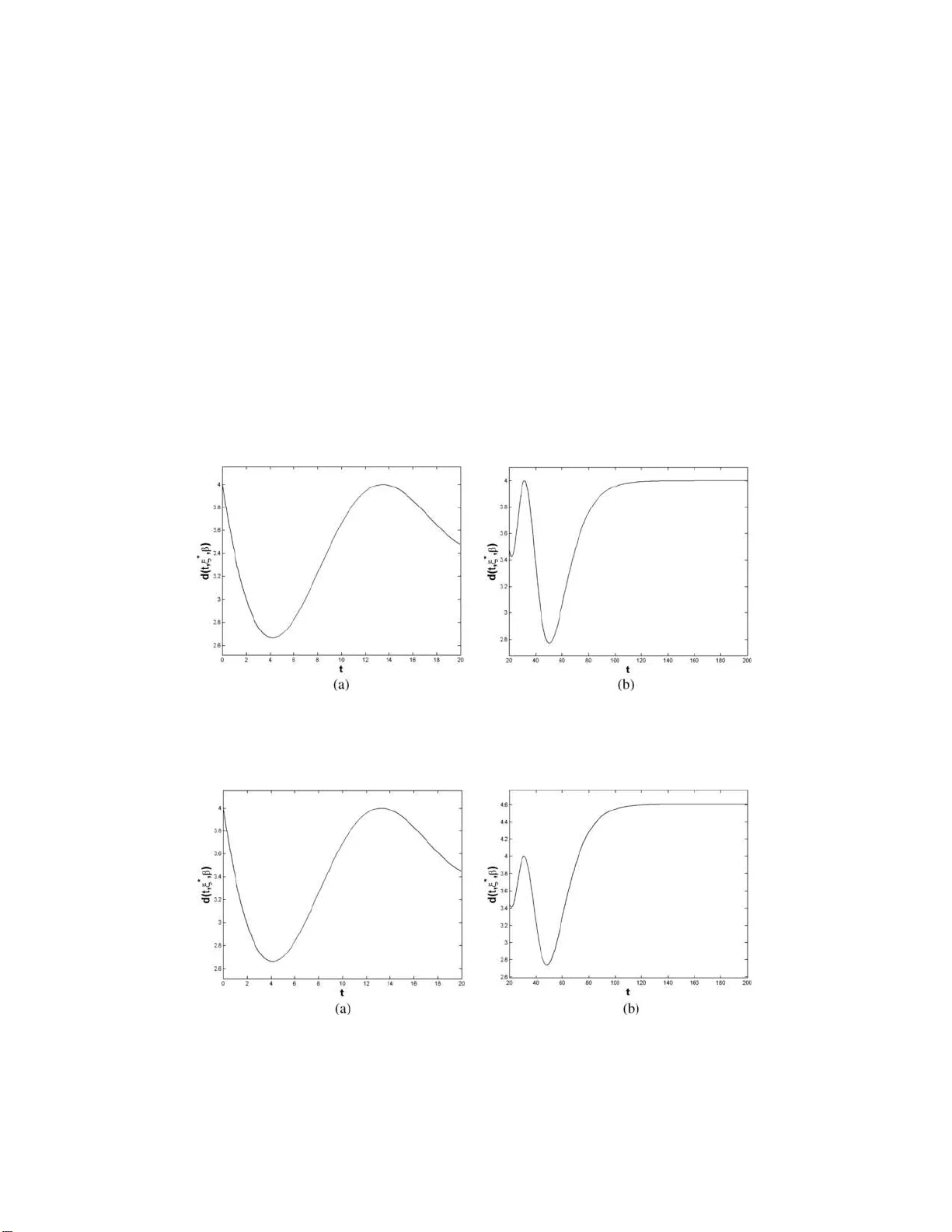
The Annals of Statistics 2008, V ol. 36, No. 1, 428–444 DOI: 10.1214 /0090536 07000000776 c Institute of Mathematical Statistics , 2 008 LOCALL Y D-OPTIMAL DESIGNS BASED ON A CLAS S OF COMPOSED MODEL S RESUL TED FR OM BLENDING EMAX AND ONE-C OMP AR TMENT MODELS 1 By X. F ang and A. S. Heda y a t University of Il linois , Chic ago A cla ss of nonlinear mod els com bining a p harmacokinetic com- partmental mod el and a pharmacody n amic Emax model is intro- duced. The locally D- optimal (LD) design for a four-parameter com- p osed model is found to b e a saturated four-p oint u n iform LD d esign with the t wo b ou n dary points of the desig n sp ace in the LD d esign supp ort. F or a five-parameter composed mod el, a sufficient condition for the LD d esign to require t he minimum num b er of sampling time p oin ts is derived. Robust LD designs are also inv estigated for b oth mod els. It is found that an LD design with k parameters is equiv alen t to an LD design with k − 1 parameters if the linear parameter in the tw o comp osed mo dels is a nuis ance parameter. A ssorted examples of LD designs are presented. 1. Introd uction. A class of m o dels is constructed b y plugging a pharma- cokinetic (PK) compartmental mo del in to a p harmaco dynamic (PD) Emax mo del. Under this class of mo dels, only one measuremen t is r equ ired p er study sub ject rather than m u ltiple measurements and b oth PK and PD pa- rameters can b e estimate d b y a single exp erimental setup. Other adv antag es of this approac h will b e listed shortly after the related PK and PD mo dels are introdu ced. A b asic PD Em ax mo del can b e expressed as E ([ D ]) = E 0 + E max [ D ] / ( E D 50 + [ D ]), wh er e E ( · ) is the dru g effe ct such as reduction in lo w-density Received Ap ril 2006; revised Marc h 2 007. 1 Supp orted by N SF Grants DMS- 01-03727, DMS-06-03761 and NIH Grant P50- A T00155 (join tly su p p orted by National Center for Complementary and A ltern ativ e Medicine, the Office of Dietary Supp lemen ts, the Office of Researc h on W omen’s Health and National In stitu te of General Medicine). Any opinions, findin gs, and conclu sions or recommendations expressed in this material are those of the authors a nd do not necessarily reflect the views of th e NS F and the NIH. AMS 2000 subje ct classific ation. 62K05. Key wor ds and phr ases. D-optimal design, pharmacokinetic compartmen tal mod el, pharmacod ynamic Emax mo del, n onlinear model. This is an electronic r eprint of the origina l article published by the Institute of Mathematica l Statistics in The Annals of Statistics , 2008, V ol. 36, No. 1, 428–44 4 . This reprint differs from the original in paginatio n and typo graphic detail. 1 2 X. F ANG AND A. S. HEDA Y A T c holesterol and [ D ] is the concen tration of free drug in the environs of the drug r eceptor. The Emax model contai ns three PD parameters. E D 50 is the drug concen tration sho wing 50% of the m axim um dr ug effect, E max is the maxim um drug effect and E 0 is the b aseline effect. F or the concept of Emax mo del, th e reader is r eferred to Ritsc hel [ 22 ]. V arious app licatio ns of Emax mo dels hav e b een discussed by , but are not limited to, Gra ve s et al. [ 7 ], Demana et al. [ 4 ], Angus et al. [ 1 ], S taab et al. [ 26 ] and Heda y at, Y an and P ezzuto [ 11 , 12 ]. Since a PK compartmenta l mo del describ es dru g concen tr ation across time, the [ D ] can b e appro ximated b y an app r opriate P K mo del. After replacing [ D ] in the Emax mo del by an op en one-compartmen t m o del with IV b olus input and first-order elimination r esults in the comp osed Emax- PK1 mo del Y tj = β 0 + β 1 · D β 2 e β 3 t + D + ε tj , (1.1) where Y tj is the effect of the drug at time t observe d on sub ject j , β 0 is the minim um resid u al effect , β 1 is the maxim um dru g effect, β 2 is the E D 50 and β 3 is the tota l eli mination rate. It is assumed that the errors across time and sub jects are i.i.d. N (0 , σ 2 ). Throughou t this p ap er, D is the administered dose in the unit of dru g amount p er unit b ody w eigh t. F or the concept and essen tial results of the one-compartmen t mo del related to IV b olus, the reader is referred to Rowland and T ozer [ 24 ], Landa w [ 16 ], Dette and Neugebauer [ 5 ], Han and Chaloner [ 8 ] and Heday at, Zh ong and Nie [ 10 ]. If [ D ] is replaced b y an op en o ne-compartment mo d el with the first-order input and th e first-order elimination, the resu lting comp osed Emax-PK2 mo del b ecomes Y tj = β 0 + β 1 · D ( e − β 2 t − e − β 3 t ) β 4 (1 − β 3 β − 1 2 ) + D ( e − β 2 t − e − β 3 t ) + ε tj , (1.2) where β 0 is th e baseline effect, β 1 is E max , β 2 is th e absorption rate, β 3 is th e total elimination rate and β 4 is the E D 50 . Th e assum p tion ab out the error terms is the same as that in mo d el ( 1.1 ). F or the concept and v arious results related to this one-compartmen t mo del, the reader is referred to Ro dda, Sampson and S mith [ 23 ], Da vidian and Gallan t [ 3 ], Mallet [ 18 ], Mandema, V erotta and Sheiner [ 19 ], V erme et al. [ 27 ], Lind sey et al. [ 17 ], Landa w [ 16 ], A tkinson et al. [ 2 ] and W ak efield [ 28 ]. Other adv antag es of the Emax-PK mo d els in clude (1) The PK p arameters can b e estimate d without dr a wing b lo o d samples. (2) Drug effec t b ecomes a function of time rather than a function of dr u g concen tration wh ic h itself is a function o f time. As a result, the drug effect is p redictable across time, suc h as blo o d pressure is b eing reduced across ti me. (3) Sampling at v arious time p oint s is con trollable b efore taking samples, whereas the drug concen tration LD DESIGN FOR COMPOSED PK /PD MODELS 3 in an Emax mo del alone is unkno wn b efore s amp ling. Therefore, one can obtain b ette r e stimates of PK and PD parameters b y implement ing suitable designs. (4) The residual effect of a drug can b e estimated at any time p oin t through the Emax-PK1 mo del. (5) Th e baseline effect of a dru g can b e estimated thr ough the Emax-PK2 mo del. In this pap er, lo cally D-optimal (LD) designs and robust LD designs for the preceding t wo Emax-PK models are studied for the pur p ose of estimat- ing all p opulation PK p arameters. Th ese PK parameters are consid er ed fixed effects although th ey lik ely d iffer b etw een s u b jects. In Section 2 , the equiv- alence theory for n onlinear mo d els is br iefly review ed. Section 3 con tains the main results ab out the n umb er of sampling time p oin ts in an LD d esign supp ort for the Emax-PK mo dels. Examples of LD designs for b oth models are pro vid ed in Sectio n 4 . S ome assorted robust LD d esigns are in v estigate d in Section 5 . Discussion and conclusion are summarized in Section 6 . 2. Pr eliminaries. T he equiv alence theorem for d esigns based on linear mo dels was first in tro d u ced and deve lop ed by K iefer and W olfo wiz [ 15 ]. White [ 29 ] extended the equiv alence theorem to lo cally optimal designs based on nonlinear mod els. In a nonlinear mod el, the Fisher information matrix d ep ends on unknown parameters. As a result, there is n o global op- timizatio n for all v alues of mod el parameters and the optimalit y of a design can b e ev aluated on ly for sp ecial v alues of mo d el parameters, called n omi- nal or p ostulated v alues. F or details, the reader is referr ed to Silvey [ 25 ] and Heda y at [ 13 ]. Without loss of generalit y , let u s consider the n onlinear mo del Y tj = η ( t, ~ β ) + ε tj with ε tj ’s b eing i.i.d. N (0 , σ 2 ). T he normalized Fisher infor- mation matrix for the en tire mod el parameters based on the design measure ξ = { ( t 1 , p 1 ) , . . . , ( t K , p K ) } can b e expressed as M ( ξ , ~ β ) = σ − 2 K X i =1 p i ∂ η ( t i , ~ β ) ∂ ~ β ∂ η ( t i , ~ β ) ∂ ~ β ′ . (2.1) A design measure ξ = { ( t 1 , p 1 ) , . . . , ( t K , p K ) } is a description of s ampling time p oin ts ( t 1 , . . . , t K ) wh ere Y t i j will b e measured for the j th s u b ject at time t i . Asso ciated with t i is the mass p i suc h that 0 < p i < 1 , and P p i = 1 . In design ξ , p 1 , . . . , p K represent the prop ortion of the num b er of sub jects studied take n at time t 1 , . . . , t K , resp ectiv ely . F or a total sample of size n , n i = n p i is the num b er of sub jects to b e stud ied at t i . F or the purp ose of obtaining the most precise estimato rs of the en tire m o del parameters, one needs to iden tify a design measure whose r elated Fisher in f ormation matrix is nonsingu lar and whose determinant is maximized in th e class of comp eting designs. T h is is b ecause M − 1 ( ξ , ~ β ) is prop ortional to the asymptotic v ariance and co v ariance matrix of the MLE of the mo d el parameters. An LD design 4 X. F ANG AND A. S. HEDA Y A T for a giv en set of parameters h as the maxim um determinant for its Fish er information matrix based on the p ostulate d v alues for these p arameters. When the n um b er of P K parameters of inte rest is s ≤ k in a k -parameter nonlinear mo d el, the asymptotic generalized v ariance of these s estimators can b e expressed as n − 1 [ M ( ξ , ~ β ) / M 22 ( ξ , ~ β )] − 1 , wh ere M 11 ( ξ , ~ β ) M 12 ( ξ , ~ β ) M 21 ( ξ , ~ β ) M 22 ( ξ , ~ β ) ! is th e partitioned form of M ( ξ , ~ β ) with M 11 ( ξ , ~ β ) b eing the asso ciated s × s information matrix of the s p arameters under the design ξ . F ollo wing White [ 29 ], the design ξ ∗ in a class of co mp eting designs, D , is said to b e an LD s design if det M ( ξ ∗ , ~ β ) / det M 22 ( ξ ∗ , ~ β ) = max ξ ∈D [det M ( ξ , ~ β ) / det M 22 ( ξ , ~ β )]. White [ 29 ] established that the design ξ ∗ is an LD s design if and only if sup t ∈T d ( t, ξ ∗ , ~ β ) = s , where d ( t, ξ , ~ β ) = tr { I ( t, ~ β ) M − 1 ( ξ , ~ β ) } − tr { I 22 ( t, ~ β ) × M − 1 22 ( ξ , ~ β ) } when s < k and d ( t, ξ , ~ β ) = tr { I ( t, ~ β ) M − 1 ( ξ , ~ β ) } when s = k and T = [0 , ∞ ) is the set of all samp ling time p oin ts with the un d erstanding that the extreme righ t time p oin t is a v ery large practitioner-sele cted time point. Here, I ( t, ~ β ) is the information m atrix for th e design w ith the supp ort p oint of t only and it is partitioned as that of M ( ξ , ~ β ). The quan tit y d ( t, ξ , ~ β ) can b e interpreted as th e v ariance of the estimated resp onse at time t w hen s = k and is th e v ariance o f the estimated resp onse after eliminating the e ffects of the k − s nuisance parameters when s < k . Before searc hing for optimal t i and p i , the r equired num b er of design p oint s in an LD design supp ort is inv estigat ed first for b oth theoretica l and practical interests. Kno wing the required num b er of design p oin ts in adv ance w ould signifi can tly reduce the task of searc hing for an LD design. 3. Main results. In this section, the supp ort size of an L D design for the Emax-PK1 mo del und er the normality assumption is in v estigated. S in ce the corresp ondin g induced design s pace, C = { σ − 1 ( ∂ η ( t, ~ β ) ∂ ~ β ) : t ∈ T } , is a b ound ed subset in R k and the determinan t of the Fisher inform ation m atrix is a con tin uous fun ction on C , th us an LD d esign for this setup must exist. In what follo w s, by a saturated d esign it is mean t a design in whic h the n umber of design time p oints is equal to the num b er of mo del parameters. Theorem 1. Under mo del ( 1.1 ): E ( Y t ) = β 0 + β 1 · D β 2 e β 3 t + D with V ar( Y t ) = σ 2 , wher e t ∈ [0 , u ] , an LD design ξ ∗ is a satur ate d D-optimal design with time 0 and u in its supp ort. Pr oof . Let M ( ξ ∗ , ~ β ) b e the Fish er information matrix for ~ β = ( β 0 , β 1 , β 2 , β 3 ) T based on an LD design ξ ∗ and define f 0 ( t ) = tr( I ( t, ~ β ) M − 1 ( ξ ∗ , ~ β )) + c , LD DESIGN FOR COMPOSED PK /PD MODELS 5 where c ∈ R is arbitrary and I ( t, ~ β ) = σ − 2 1 D ( β 2 e β 3 t + D ) − 1 − β 1 D e β 3 t ( β 2 e β 3 t + D ) − 2 − β 1 D β 2 te β 3 t ( β 2 e β 3 t + D ) − 2 × 1 D ( β 2 e β 3 t + D ) − 1 − β 1 D e β 3 t ( β 2 e β 3 t + D ) − 2 − β 1 D β 2 te β 3 t ( β 2 e β 3 t + D ) − 2 T . It can b e sho wn that f 0 ( t ) has the same n umber of zeros as f ( t ) = a 40 e 4 β 3 t + e 3 β 3 t ( a 31 t + a 30 ) + e 2 β 3 t ( a 22 t 2 + a 21 t + a 20 ) + e β 3 t ( a 11 t + a 10 ) + a 00 , wh ere a ij dep end s on ξ ∗ , D and β k , i ∈ { 0 , 1 , 2 , 3 , 4 } , j ∈ { 0 , 1 , 2 } , k ∈ { 1 , 2 , 3 } . No- tice that a 22 > 0 and a 31 < 0 since th e cofa ctor Cof 14 in M − 1 is p ositiv e ( App end ix ). Also, by the Remark in the App end ix , it can b e s ho wn that a 11 > 0 . No w in order to p ro v e that f ( t ) has at most six zeros, the prop er- ties of v arious d eriv ativ es of f ( t ) will b e explored. By differentiat ing f ( t ) with resp ect to t , one h as f ′ ( t ) = 4 β 3 a 40 e 4 β 3 t + e 3 β 3 t (3 β 3 a 31 t + b 30 ) + e 2 β 3 t (2 β 3 a 22 t 2 + b 21 t + b 20 ) + e β 3 t ( β 3 a 11 t + b 10 ) , where the b ij ’s are the corresp ondin g constan ts. Af ter setting f ′ ( t ) = 0 and m ultiplying b oth sides of f ′ ( t ) = 0 by e − 4 β 3 t , one obtains ˜ f ′ ( t ) = 4 β 3 a 40 + e − β 3 t (3 β 3 a 31 t + b 30 ) + e − 2 β 3 t (2 β 3 a 22 t 2 + b 21 t + b 20 ) + e − 3 β 3 t ( β 3 a 11 t + b 10 ) . Notice th at f ′ ( t ) and ˜ f ′ ( t ) ha v e the same num b er of zeros. After d ifferen ti- ating ˜ f ′ ( t ), one has ˜ f ′′ ( t ) = e − β 3 t ( − 3 β 2 3 a 31 t + c 30 ) + e − 2 β 3 t ( − 4 β 2 3 a 22 t 2 + c 21 t + c 20 ) + e − 3 β 3 t ( − 3 β 2 3 a 11 t + c 10 ) , where c ij ’s are the corresp ondin g constant s. By m ultiplying ˜ f ′′ ( t ) by e 3 β 3 t , one has ˜ ˜ f ′′ ( t ) = e 2 β 3 t ( − 3 β 2 3 a 31 t + c 30 ) + e β 3 t ( − 4 β 2 3 a 22 t 2 + c 21 t + c 20 ) + ( − 3 β 2 3 a 11 t + c 10 ) . Differen tiating ˜ ˜ f ′′ ( t ) yields ˜ ˜ ˜ f ′′′ ( t ) = e 2 β 3 t ( − 6 β 3 3 a 31 t + d 30 ) + e β 3 t ( − 4 β 3 3 a 22 t 2 + d 21 t + d 20 ) − 3 β 2 3 a 11 , 6 X. F ANG AND A. S. HEDA Y A T where d ij ’s are th e corr esp onding constants. Next, it will be sho wn that the function g ( t ) = e 2 β 3 t ( − 6 β 3 3 a 31 t + d 30 ) + e β 3 t ( − 4 β 3 3 a 22 t 2 + d 21 t + d 20 ) has at most three stationary p oin ts. By multiplying b oth sides of g ′ ( t ) = 0 b y e − 2 β 3 t , one h as ˜ g ′ ( t ) = − 12 β 4 3 a 31 t + e 30 + e − β 3 t ( − 4 β 4 3 a 22 t 2 + e 21 t + e 20 ) = 0 , where e ij ’s are th e corresp ondin g constan ts. Setting ˜ g ′′ ( t ) = 0, one has e − β 3 t (4 β 5 3 a 22 t 2 + f 21 t + f 23 ) = 12 β 4 3 a 31 , (3.1) where f ij ’s are the co rresp onding constan ts. S ince the left-hand side of ( 3.1 ) has at m ost t w o s tationary p oint s an d it approac hes 0 ab ov e the t axis as t go es to ∞ , the m ost right monotone interv al of th e left-hand sid e will not in tersect the h orizon tal line y = 12 β 4 3 a 31 , wh ic h is b elo w the t axis. Th er efore, ( 3.1 ) has at most tw o ro ots. No w, since ( 3.1 ) has at most t wo ro ots, ˜ g ′ ( t ) will ha v e at most three zeros. This implies that g ( t ) has at m ost three stationary p oints. Since g ( t ) goes to 0 b elo w the t axis as t go es to −∞ and 3 β 2 3 a 11 > 0, th e most left monotone in terv al will not inte rsect the horizon tal line y = 3 β 2 3 a 11 , whic h is ab o v e the t axis. Consequently , ˜ ˜ ˜ f ′′′ ( t ) has at most three zeros. This implies that ˜ f ′′ ( t ) has at most four zeros and f ′ ( t ) has a t most fi v e zeros. As a result, f ( t ) has at most six zeros. Since f ( t ) h as at most six zeros for all c ′ s and by the equiv alence theorem the interior p oints of an LD design m ust b e lo cally maxim um p oin ts of tr( I ( t, ~ β ) M − 1 ( ξ ∗ , ~ β )), therefore there are at most t wo optimal design p oin ts on (0 , ∞ ) . Otherwise, f ( t ) has more than six zeros for some c . Since the induced design p oin t at time 0 is not p rop ortional to that at time u > 0, the existence of an LD design based on model ( 1.1 ) forces the t w o b oundary p oint s to b e in the optimal d esign su pp ort. Theorem 1 demonstrates that an LD design for mo del ( 1.1 ) is of the form ξ ∗ = { (0 , 1 / 4 ) , ( t 2 , 1 / 4) , ( t 3 , 1 / 4) , ( u, 1 / 4) } o ve r t ∈ [0 , u ]. Consequentl y , to searc h for an LD design for mo d el ( 1.1 ), one only needs to find out t 2 and t 3 . Theorem 2. A n LD design for the E max-PK2 mo del has minimum supp ort size with time p oint 0 in its supp ort if d ( t, ξ , ~ β ) has pr e cisely four lo c al ly maximum time p oints when t ∈ (0 , ∞ ) . Pr oof . By Carath ´ eo dory’s theorem [ 25 ], for this five-paramete r nonlin- ear mo del, an LD d esign must hav e at least fiv e time p oin ts in its supp ort. LD DESIGN FOR COMPOSED PK /PD MODELS 7 By the equiv alence theorem, LD design time p oin ts m ust b e necessarily the lo cally maxim um points of d ( t, ξ , ~ β ) when t ∈ (0 , ∞ ) . S ince d ( t, ξ , ~ β ) has four lo cally maxim um time p oin ts and the in d uced design time p oin ts at t = 0 and t = ∞ are th e same, the existence of an LD design forces time p oin t 0 and the four lo cally maxim um p oin ts to b e in the d esign supp ort. Theorem 2 pro vid es a sufficien t condition for an LD design for the Emax- PK2 mo del to b e minimally supp orted when the original design space is [0 , ∞ ) . In general, if the required n um b er of L D sampling time p oints is un- kno wn for a k -p arameter nonlinear mo d el, the practitioner could searc h for the b est k -p oin t un iform LD design fir st. Then the V-algorithm by F edorov [ 6 ] can b e applied to searc h for an LD design with the k -p oin t u n iform LD design as the initial d esign. When β 0 is a nuisance parameter, it is found th at an LD design is also an LD k − 1 design for a k -paramete r nonlinear mo del of the form y tj = β 0 + ˜ η ( t, ~ β ) + ε tj , where ε tj are i.i.d. N (0 , σ 2 ) and ∂ ˜ η ( t, ~ β ) /∂ β i is not free of β i for i = 1 , . . . , k − 1. F or a mo del of this form, the follo wing result is obtained. Theorem 3. A n LD design for the k -p ar ameter nonline ar mo del is also an LD k − 1 design for p ar ameters β 1 , . . . , β k − 1 . The p ro of is based on the fact that b oth I 22 in I ( t, ~ β ) an d M − 1 22 in M ( ξ ∗ , ~ β ) are equal to 1. Theorem 3 sho ws that the LD k − 1 design is globally optimized for β 0 although it is o nly locally o ptimal for the o ther nonlinear parameters. Theorem 3 is applicable to b oth Emax-PK mo dels discussed in this pap er. Examples of LD k − 1 designs originated fr om LD designs f or b oth Emax-PK1 and Emax-PK2 mo dels are giv en in Section 4 . 4. Illu s trated examp les. Maximizing the determinan t of the Fisher in- formation matrix u nder nonlinear mo d els requires the forekno wledge of the v alues of mo del parameters. In practice, a goo d guess can b e obtained from a pilot exper im ent. F or examp le, su pp ose based on the prior information from the pilot exp erimen t, th e minimum residual effect is equal to 0 . 5, the maxim um d rug effect is equal to 10, the E D 50 is equal to 1 mg / kg and the total elimination r ate is equal to 0.1 hour − 1 . T h e search for an LD design generally con tains t w o steps: (1) finding a b est k -p oin t u niform LD design; (2) using the V-algorithm (F edoro v [ 6 ]) to fi nd an LD design giv en the ini- tial d esign as that foun d in step (1). F or the Emax-PK2 mo del, a searc h as describ ed w as p er f ormed. How ever, for the Emax-PK1 mod el, the searc h w as stopp ed at step (1) since T heorem 1 sho ws that an LD design for this mo del is a saturated LD design. F or the Emax-PK1 mo del with p ostulated ~ β = (0 . 5 , 10 , 1 , 0 . 1) and an ini- tial dose of 5 mg / kg, a f our-p oint LD design is found to b e un iform at 8 X. F ANG AND A. S. HEDA Y A T times 0, 13 . 48, 31 . 62 and 160 . 00 hou r s. Figure 1 illustrates some essen tial c haracteristics of d ( t, ξ , ~ β ) for this design. If the maximum s ampling time is 72 or 24 hours, then the LD design can b e found to b e uniform at times 0 , 13 . 26, 31 . 0 5 and 72 hours or at times 0, 7 . 97, 17 . 83 and 24 hours, resp ectiv ely . T h e d ( t, ξ , ~ β ) for these t w o designs are illustrated in Figures 2 and 3 . Although th e upp er b ound of the supp ort size for an LD design b ased on the Emax-PK2 mo del is 16 by Carath ´ eo dory’s theorem, one can s till follo w the t w o-step searc h describ ed ab o v e. F or the Emax-PK2 mo d el with p ostulated ~ β = (0 . 5 , 10 , 0 . 5 , 0 . 1 , 1), an LD design is found to b e uniform at Fig. 1. Plots of d ( t, ξ ∗ , ~ β ) with (a) t ∈ [0 , 20] and (b) t ∈ [20 , 200] , r esp e c- tively. The design sp ac e i s [0 , ∞ ) and the optimal sampli ng times ar e found at 0 , 13 . 481 506 , 31 . 624511 , 160 . 00199 . The initial I V dose is 5 mg / kg . Fig. 2. Plots of d ( t, ξ ∗ , ~ β ) with (a) t ∈ [0 , 20] and (b) t ∈ [20 , 200] , r esp e ctively. The design sp ac e i s [0 , 72] hours and the optimal sampl i ng times ar e found to b e at 0 , 13 . 263 029 , 31 . 050686 and 72 hours. LD DESIGN FOR COMPOSED PK /PD MODELS 9 times 0, 0 . 27 5, 2 . 999, 14 . 75 and 32 . 7 hou r s. The asso ciated d ( t, ξ , ~ β ) for this design is illustrated in Figure 4 . 5. Rob u st designs. Applying an LD design in pr actice ma y b e critic ized for its lo cal optimalit y . If the nomin al v alues of the mod el parameters are n ot close to th e true v alues, a m ore desirable design w ould b e a robus t design, whic h w ould lead to a b etter p arameter estimation than an LD design while main taining high efficiency . The relativ e efficiency of a design ξ compared to an LD design ξ ∗ for the p ostulated ~ β is defined as det ( ξ , ~ β ) / det ( ξ ∗ , ~ β ). A robu st in dex d efined as | ( ∂ (det M ( ξ , ~ β )) /∂ β i ) − 1 | for p arameter β i , i = 0 , 1 , . . . is intro d uced to compare the robustness of LD designs based on differen t nominal v alues of the mo del p arameters. F or a linear m o del, this robust in dex is ∞ , indicating th at an L D design is globally optimal f or all v alues of the mo del parameters. Ho w ev er, for a nonlinear mo del, it measures the inv erse of the c hanging rate of the determinan t in the neigh b orho od of the p ostulated ~ β . Therefore, it is ca lled the lo cally rob u st index (LRI ). The larger the v alue of the LRI , the m ore lo cally r obust the d esign. One class of robust designs is the equally spaced uniform L D (ESULD) designs. An adv anta ge of this class of designs is that it can b e implemen ted v ery easily . It is robust for the estimation of parameters in the mo dels that w ere describ ed in Heday at, Y an and Pezzuto [ 11 , 12 ] and Heda y at, Zh on g and Nie [ 10 ]. The class of ESULD designs is examined here for b oth Emax- PK1 and Emax-PK2 mo d els. T able 1 sho ws th at an ESULD design retains its robustness but loses its efficiency as the size of the d esign supp ort increases. F or practical applications, the fi v e- or the six-p oin t ESULD designs are recommended. Since the efficiency of the ESULD designs is v ery low for th e Emax-PK2 mo del, another class of robust designs is constructed based on an LD design. Fig. 3. Plot of d ( t, ξ ∗ , ~ β ) when th e design sp ac e is [0 , 24] hours b ase d on the Emax-PK1 mo del. 10 X. F ANG AND A. S. HEDA Y A T T able 1 ESULD designs for the mo del with the initial dose = 5 mg / kg and the nominal values β 1 = 10 , β 2 = 1 mg / kg , β 3 = 0 . 1 h − 1 Supp ort size Supp ort of ξ Efficiency of ξ LRI for β 1 LRI for β 2 LRI for β 3 4 0 , 13 . 48 , 31 . 62 , 160 . 00 1 0 . 95901654 0 . 10344687 0 . 01918 7232 5 0 , 16 . 176 × i, i = 1 , 2 , 3 , 4 0 . 47637398 9 2 . 0131589 0 . 19911378 0 . 04025 6987 6 0 , 14 . 736 × i, i = 1 , 2 , 3 , 4 , 5 0 . 48103875 5 1 . 9936368 0 . 20439842 0 . 03987 6038 7 0 , 13 × i, i = 1 , 2 , . . . , 6 0 . 44068661 3 2 . 1761871 0 . 22903063 0 . 04384 4867 8 0 , 11 . 094 × i, i = 1 , 2 , . . . , 7 0 . 40311946 6 2 . 3789884 0 . 25133456 0 . 04758 0261 9 0 , 9 . 647 × i, i = 1 , 2 , . . . , 8 0 . 37613241 7 2 . 549678 0 . 26807298 0 . 05098 9122 10 0 , 8 . 558 × i, i = 1 , 2 , . . . , 9 0 . 355042 847 2 . 701129 0 . 282684 01 0 . 05401 8207 11 0 , 7 . 686 × i, i = 1 , 2 , . . . , 10 0 . 3379349 2 . 8378736 0 . 29572619 0 . 05676 2451 12 0 , 7 × i, i = 1 , 2 , . . . , 11 0 . 323818285 2 . 9615886 0 . 30723535 0 . 0586 53795 When s = 4, t he design is the LD design. LD DESIGN FOR COMPOSED PK /PD MODELS 11 Fig. 4. Plots of d ( t, ξ ∗ , ~ β ) with (a) t ∈ [0 , 0 . 5] , (b) t ∈ [0 . 5 , 20] , (c) t ∈ [20 , 60] and (d) t ∈ [60 , 200] , r esp e ctively. The numeric al solutions of the lo c al maximums ar e 0 , 0 . 275 , 2 . 999 , 14 . 75 , 32 . 695 . The i nitial dos e is 5 mg / kg . The supp ort of suc h a r ob u st d esign includes all th e design time p oin ts of an LD design as w ell as the design time p oints in the form of t ∗ + r or t ∗ − r , where t ∗ is a design time p oin t of an LD design and r is a fixed n umber . F or con v enience, this class of designs is referred to as equal-step expanded uniform LD (ESEULD) d esigns. F or example, if an LD design is ξ ∗ = t 1 t 2 t 3 1 / 3 1 / 3 1 / 3 , then a four-p oint ESEULD design wo uld b e ξ ∗∗ = t 1 t 1 + r t 2 t 3 1 / 4 1 / 4 1 / 4 1 / 4 ; a five-point ESEULD design w ould b e ξ ∗∗ = t 1 t 1 + r t 2 t 2 + r t 3 1 / 5 1 / 5 1 / 5 1 / 5 1 / 5 ; 12 X. F ANG AND A. S. HEDA Y A T Fig. 5. The efficiency of a ESEULD design versus step length r b ase d on (a) Emax-PK1 mo del and (b) Em ax-PK2 mo del. a six-p oin t ESEULD d esign w ould b e ξ ∗∗ = t 1 t 1 + r t 2 t 2 + r t 3 − r t 3 1 / 6 1 / 6 1 / 6 1 / 6 1 / 6 1 / 6 and a sev en-p oint ESEULD design would b e ξ ∗∗ = t 1 t 1 + r t 2 − r t 2 t 2 + r t 3 − r t 3 1 / 7 1 / 7 1 / 7 1 / 7 1 / 7 1 / 7 1 / 7 . Since the relativ e efficiency of the design ξ ∗∗ relativ e to an LD design ξ ∗ , det M ( ξ ∗∗ , ~ β ) / det M ( ξ ∗ , ~ β ), is a function of r giv en ξ ∗ and ~ β , it is imp ossible to giv e an explicit form of r as a fun ction of efficiency . Ho w ev er, it is p ossible to plot efficiency v ersus step length r to find out the n umerical relationship b et we en r and the efficiency . Figure 5 (a) and 5 (b) sho ws such p lots based on the Emax-PK1 mod el and the Emax-PK2 mo d el, resp ectiv ely . Th e same p ostulated v alues of β i ’s as those in S ection 4 are u s ed for illustrations and tables thr ou gh ou t this section. F rom this figure, it is clear that th e v alue of r cannot b e assigned arbitrarily for some n -p oin t ESEULD designs. F or example, r = 0 . 95 do es not exist for a five- p oin t ES EULD design based on th e Emax-PK1 mo del. I n this figure, r = 1 h our and r = 0 . 2 h our are c hosen for r obustness study based on the Emax-PK1 mo del and the Emax- PK2 mod el, resp ectiv ely . The c orresp onding design time p oin ts are listed in T ables 2 a nd 3 . T he LRI’s are calc ulated and listed in T ables 4 and 5 . F rom these results, it app ears that the higher the relativ e efficiency of a robust LD design, the less the robustness of the d esign. 6. C onclusion an d discussion. This pap er introd uced a class of m o dels b y b lend ing a PD Emax mo del and a PK compartmental mo del and s tu died LD DESIGN FOR COMPOSED PK /PD MODELS 13 some imp ortan t features of LD, ESULD and ESEULD designs for the Emax- PK1 and the Emax-PK2 mo dels in this class. F or Emax-PK1 model, an LD design is a saturated four-p oint uniform LD design w ith the tw o b oundary time p oints of the design sp ace in its supp ort. Both time 0 and the up p er b ound of the d esign space are the infor- mativ e time p oints here. This can b e observe d d ir ectly fr om the mo del. As t appr oac h es ∞ , the Em ax-PK1 mo del is red uced to Y tj = β 0 + ε tj . There- fore, the up p er b ound of the design space is an informativ e time p oint for T able 2 ESEULD designs b ase d on the Emax-PK1 mo del with r = 1 hour Supp ort size ESEULD design p oint 4 0 , 13 . 48 , 31 . 62 , 160 . 00 5 0 , 1 , 13 . 48 , 31 . 62 , 160 . 00 6 0 , 1 , 13 . 48 , 14 . 48 , 31 . 62 , 160 . 00 7 0 , 1 , 13 . 48 , 14 . 48 , 31 . 62 , 32 . 62 , 160 . 00 8 0 , 1 , 13 . 48 , 14 . 48 , 31 . 62 , 32 . 62 , 159 , 160 . 00 9 0 , 1 , 12 . 48 , 13 . 48 , 14 . 48 , 31 . 62 , 32 . 62 , 159 , 160 . 00 10 0 , 1 , 12 . 48 , 13 . 48 , 14 . 48 , 30 . 62 , 31 . 62 , 32 . 62 , 15 9 , 160 . 0 0 T able 3 ESEULD designs b ase d on the Emax-PK2 mo del with r = 0 . 2 hour Supp ort size ESEULD design p oints 5 0 , 0 . 275 , 2 . 999 , 14 . 75 , 32 . 695 6 0 , 0 . 275 , 0 . 475 , 2 . 999 , 14 . 75 , 32 . 695 7 0 , 0 . 275 , 0 . 475 , 2 . 999 , 3 . 199 , 14 . 75 , 32 . 695 8 0 , 0 . 275 , 0 . 475 , 2 . 999 , 3 . 199 , 14 . 75 , 14 . 95 , 32 . 695 9 0 , 0 . 275 , 0 . 475 , 2 . 999 , 3 . 199 , 14 . 75 , 14 . 95 , 32 . 495 , 32 . 69 5 10 0 , 0 . 275 , 0 . 475 , 2 . 799 , 2 . 999 , 3 . 199 , 14 . 75 , 14 . 95 , 32 . 495 , 32 . 69 5 T able 4 Efficiency and r obustness of ESEULD designs for the Emax-PK1 mo del ESEULD design Efficiency of ξ LRI: β 1 LRI: β 2 LRI: β 3 4-p oint 1 0 . 95901654 0 . 10344687 0 . 01918 7232 5-p oint 0 . 7588 1 . 2638471 0 . 13584 7 0 . 02557 6467 6-p oint 0 . 7284 1 . 3165725 0 . 13967 382 0 . 025674003 7-p oint 0 . 7846 1 . 2223363 0 . 12857 595 0 . 021936078 8-p oint 0 . 9193 1 . 0431845 0 . 10970 443 0 . 018685843 9-p oint 0 . 8583 1 . 1172873 0 . 11907 55 0 . 02090 1414 10-p oin t 0 . 8437 1 . 1366831 0 . 12194 774 0 . 022945661 14 X. F ANG AND A. S. HEDA Y A T T able 5 Efficiency and r obustness of ESEULD designs for the Emax-PK2 mo del ESEULD design Efficiency of ξ LRI: β 1 LRI: β 2 LRI: β 3 LRI: β 4 5-p oint 1 0 . 30678 54 0 . 04648941 3 0 . 0090 373459 0 . 043066663 6-p oint 0 . 7667 0 . 40014 335 0 . 05 5507767 0 . 01177785 2 0 . 058844405 7-p oint 0 . 6995 0 . 43857 707 0 . 059457229 0 . 01300157 8 0 . 064883822 8-p oint 0 . 7168 0 . 42799 782 0 . 05768681 0 . 0126 43369 0 . 06318 0006 9-p oint 0 . 7952 0 . 38580 638 0 . 052011575 0 . 01157192 7 0 . 057033582 10-p oin t 0 . 6995 0 . 43858 02 0 . 05958319 9 0 . 0130975 78 0 . 06485593 9 parameter β 0 . When t = 0 , the mo d el is redu ced to Y tj = β 0 + β 1 D β 2 + D + ε tj . Consequent ly , time 0 is an informativ e time p oin t for β 0 as w ell as the r atio of β 1 /β 2 . A sufficien t condition for the Emax-PK2 mo del to b e minimally supp orted is giv en. Time 0 is an inform ative time p oin t here. This also can b e explained from the Emax-PK2 m o del directly . As time goes to 0, the Emax-PK2 mo del is r ed uced to Y tj = β 0 + ε tj . When β 0 is considered as a nuisance parameter, an LD d esign and an LD k − 1 design based on an y of the Emax-PK mo d els are equiv alen t. T he corresp ondin g LD design is global ly optimal for the linear parameter β 0 and lo cally optimal for the other nonlinear parameters. F uture researc h for the Emax-PK models could in vo lve random effects for certain PK parameters since these parameters lik ely differ b et wee n sub jects. The reader is referred to Men tre, Mallet and Baccar [ 20 ], P almer and Muller [ 21 ], Han and Ch aloner [ 9 ] for recen t r esults in th is area. APPENDIX: PROOFS Cof 14 of M ( ξ ∗ , ~ β ) − 1 is p ositiv e and Cof 24 of M ( ξ ∗ , ~ β ) − 1 is negativ e. Since the Fisher information matrix of ~ β = ( β 0 , β 1 , β 2 , β 3 ) T at sampling time t i for an LD design ξ ∗ = t 1 t 2 ... t s p 1 p 2 ... p s based on mo d el ( 1.1 ) or the Emax-PK1 mo d el is I ( t i , ~ β ) = σ − 2 p i 1 D ( β 2 e β 3 t i + D ) − 1 − β 1 D e β 3 t i ( β 2 e β 3 t i + D ) − 2 − β 1 D β 2 t i e β 3 t i ( β 2 e β 3 t i + D ) − 2 × 1 D ( β 2 e β 3 t i + D ) − 1 − β 1 D e β 3 t i ( β 2 e β 3 t i + D ) − 2 − β 1 D β 2 t i e β 3 t i ( β 2 e β 3 t i + D ) − 2 T , LD DESIGN FOR COMPOSED PK /PD MODELS 15 the Cof 14 has th e same sign as − det m 14 = − det s X i =1 p i D ( β 2 e β 3 t i + D ) s X i =1 p i D 2 ( β 2 e β 3 t i + D ) 2 s X i =1 p i − D 2 β 1 e β 3 t i ( β 2 e β 3 t i + D ) 3 s X i =1 p i − Dβ 1 e β 3 t i ( β 2 e β 3 t i + D ) 2 s X i =1 p i − D 2 β 1 e β 3 t i ( β 2 e β 3 t i + D ) 3 s X i =1 p i D 2 β 2 1 e 2 β 3 t i ( β 2 e β 3 t i + D ) 4 s X i =1 p i − Dβ 1 β 2 t i e β 3 t i ( β 2 e β 3 t i + D ) 2 s X i =1 p i − D 2 β 1 β 2 t i e β 3 t i ( β 2 e β 3 t i + D ) 3 s X i =1 p i D 2 β 2 1 β 2 t i e 2 β 3 t i ( β 2 e β 3 t i + D ) 4 . Let g ( t i , t j , t k ) = det D ( β 2 e β 3 t i + D ) D 2 ( β 2 e β 3 t j + D ) 2 − D 2 β 1 e β 3 t k ( β 2 e β 3 t k + D ) 3 − D β 1 e β 3 t i ( β 2 e β 3 t i + D ) 2 − D 2 β 1 e β 3 t j ( β 2 e β 3 t j + D ) 3 D 2 β 2 1 e 2 β 3 t k ( β 2 e β 3 t k + D ) 4 − D β 1 β 2 t i e β 3 t i ( β 2 e β 3 t i + D ) 2 − D 2 β 1 β 2 t j e β 3 t j ( β 2 e β 3 t j + D ) 3 D 2 β 2 1 β 2 t k e 2 β 3 t k ( β 2 e β 3 t k + D ) 4 ∀ i < j < k ≤ s , then the dete rminant o f m 14 is det m 14 = P i 0. Next, C of 24 < 0 will b e sh o wn. By the same argument, it can b e pro v ed that Cof 24 = X i 0 , this yields Cof 24 < 0. Remark. − Cof 14 − Cof 24 = − X i
Original Paper
Loading high-quality paper...
Comments & Academic Discussion
Loading comments...
Leave a Comment