A Queueing System for Modeling a File Sharing Principle

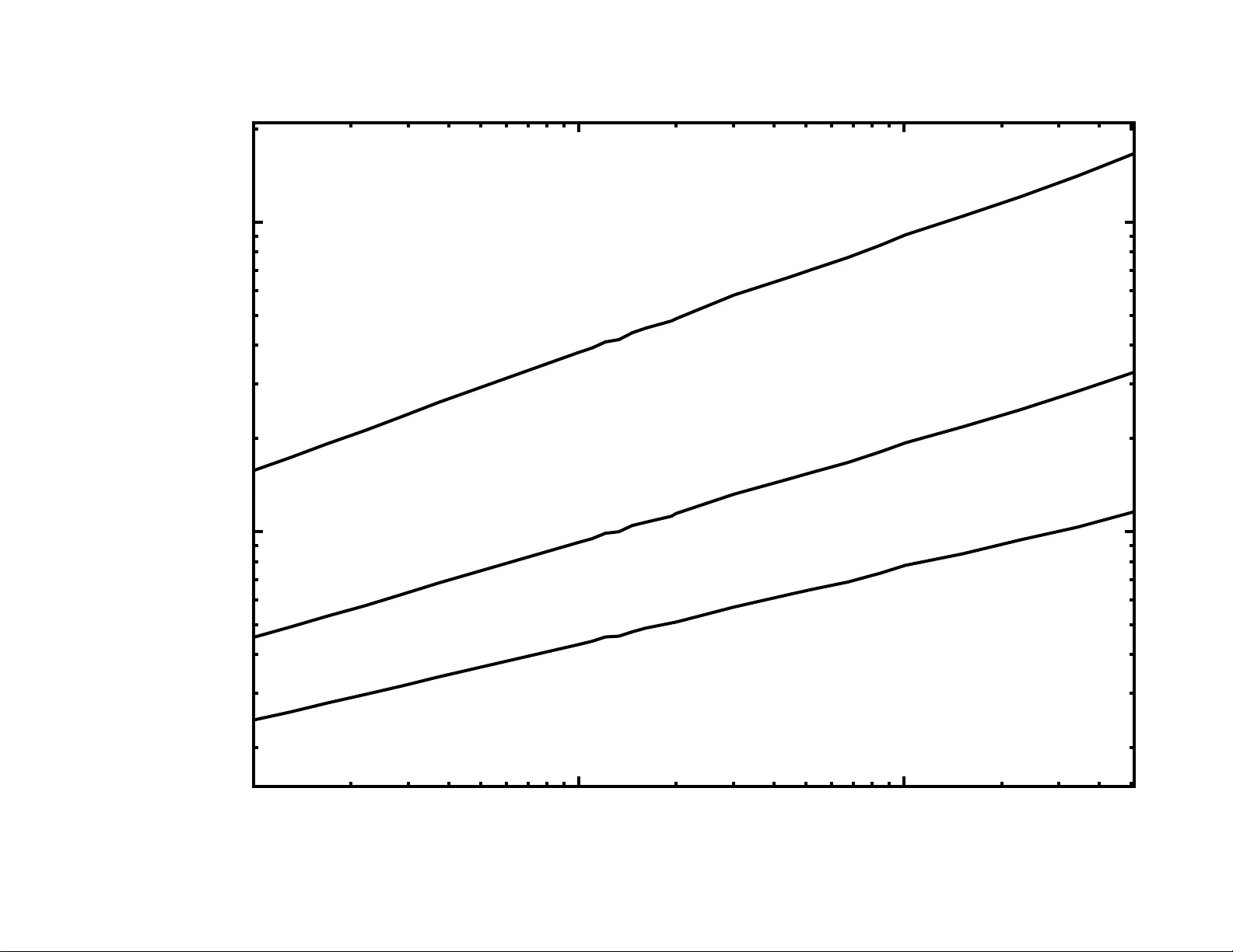
A Queueing System f or Modeling a File Sharing Principle Florian Simatos and Philippe Rober t INRIA, RAP project Domaine de V oluceau, Rocquencour t 78153 Le Chesna y , F rance {Florian.Simatos ,Philippe .Rober t}@inria.fr F a brice Guillemin Orange Labs 2, A v enue Pierre Marzin 22300 Lannion F a brice.Guillemin@or ange-ftgr oup .com ABSTRA CT W e inv estigate in this pap er the performance of a simple file sharing principle. F or this purp ose, w e consider a sys- tem composed of N p eers b ecoming active at expon ential random times ; th e system i s initia ted with only one server offering the desired file and the other peers after becoming active try to d o wnload it. Once the file h as b een downloa ded by a p eer, th is one immediately b ecome s a server. T o inves- tigate the transien t b eha vior of this file sharing system, w e study th e instan t when the system shifts from a congested state where all serv ers av ailable are saturated b y incoming demands to a state where a gro wing number of servers are idle. In spite of its apparent simplicity , this queueing mo del (with a random num b er of servers) turns out to b e q uite dif- ficult to analyze. A form ulation in terms of an urn and b a ll mod el is prop os ed and correspon d ing scaling results are de- rived. These asympt otic results are then compared against sim ulations. Categories and Subject Descriptors C.4 [ Computer Sy stems Organization ]: Perfor mance of Systems— mo deling te chniques, p erformanc e attributes General T erms Queueing Systems, T ransient A nal ysis of Marko v Processes, File S h ari ng, Peer to Peer 1. INTR ODUCTION This paper analyzes the p erforma nce of a simple file shar- ing principle d u ring a flash crowd scenario when a p opular conten t b ecomes av ailable on a p eer-to-p eer netw ork. It is supp osed that a given p eer is wi lling to share a given fi l e with a community of N peers, which are initially asleep. An asleep peer b ecomes activ e at some random time, i.e., it tries to download the file from a p eer ha ving the complete file. Once a p eer has d o wnloaded the file, it immediately becomes a server from which another p eer can downlo ad the file. T o simplify the mo del, w e assume that the file is in one piece SIGMETRICS’08, June 2–6, 2008, Annapolis, Maryland, USA. and not segmen ted in to c hunks; the t i me needed to d o wn- load the file from one serv er is supposed to be random in order t o take into account th e diversit y of upload capacities of p eers. The goal of this paper is to understand how th e netw ork builds u p in this situation as p eers join the system. In par- ticular, w e are interested in analyzing the growth of the num- b er of a v ailable serv ers in the system. Note th a t there are even tually as many serv ers as p eers since eac h of them can complete the fi le d o wnload. In spite of its apparent simplicit y , the analysis of the system is quite difficult b eca use w e have to cope with a n et w ork comprising a rand o m number of servers: When p eers com- plete their do wnload, they b ecome new servers so that the num b er of servers is contin ually increasing. It is assumed that an incoming p eer c ho oses a serv er with the smallest num b er of qu eu ed p eers. Other rout in g p olicies are consid- ered at th e end of this pap er. The analysis p erformed in this pap er substantial ly differs from earlier studies app eared so far in the tec hnical litera- ture in the sense that we consider t he transient formation of a netw ork of p ee rs. Y ang and de V eciana [17] considered a similar setting which they analyzed with results related to branching processes to describ e the exp onen tial gro wth of the number of servers. Our goal in th is pap er is precisely to obtain more detailed asymptotics of th i s transient regime. Except the p aper by Y ang and de V eciana [17], most of the pap ers pu blis hed so far on th e p erformance of p eer-to-peer systems assume that p eers joi n and leav e the system and that a steady state regime exists. The problem is then to ev aluate the impact of some p arameters of the fi le sharing protocol on the equilibrium of the system. Different tec h- niques can b e used to p erf orm such an analysis, for instance by using a Marko vian c hain to describ e the state of the sys- tem, possibly by using app ro x i mation techniques when the state space related to the number of peers in the system is too larg e. See Ge et al. [7 ]. A fluid fl o w analysis with an underlying Marko v i an structure is p ro p osed in Cl´ evenot and Nain [5] in order to mo del the Sq uirrel p ee r-to-p eer caching system. In Qiu and Srik an t [14], the authors directly use a fluid approximati on to study the steady state of a peer to p eer netw ork, subsequ en tly complemented by diffusion va ri- ations around the steady state solutions. In Massouli ´ e and V o jno vi´ c [13], the authors stu dy the p erformance of a fi le sharing system via a stochastic coup on replication form ula- tion, a coup on corresp onding to a chunk of a file. The goal of th i s study is to understand the impact of th e p olicy ap- plied b y users for choosing coup ons on the performance of the system. The system is studied in equilibrium as in Qiu and Srik ant [14]. The rest of this pap er is organized as follow s: In Section 2 , w e describe the system und er co nsideration and some h euris- tics to study the system are presen ted. I t turns out t hat the dynamics of th e system can b e decomp osed in tw o regimes. In the first one, there are almost no empty servers and we establish an analogy with a random urn and b al l problem on the real line. By approximating the p ro bability of se- lecting an urn by its mean v alue, w e analyze in Section 3 the corresp onding deterministic urn and ball problem. The analysis for the random urn and ball prob lem is muc h more complicated to analyze. The complete analysis is done in [12] and only the main results are summarized in Section 5. In Section 6, w e sup port via simulation the different approx- imations and heu ris tics made in this pap er to analyze the file sharing system. Concluding remarks are presen ted in Section 7. 2. MODEL DESCRIPTION 2.1 Pr oblem formulation W e consider throughout this p a p er a system composed of N p eers interested in do wnloading a giv en file. At the b e- ginning, only one peer (th e initial server) has the file and other peers are asleep. Wh en b eco ming active , after an ex- p onen tially distributed duration of time with parameter ρ , a peer tries to downloa d the file from the serv er t hat is th e less loaded in terms of number of queued p eers. In partic- ular, t h e first p eer b ecoming active d o wnloads the file from the initial server. The time needed to do wnload the file is assumed to be expon entially distributed with m ean 1. Expone nti al distributions. The hypothesis on the distri- bution on the duration of the t ime for a p eer t o b e active is quite reasonable: this is a classical situation when a large num b er of indep endent u se rs may access some n et work. The assumption on the duration of the time to download is not realistic in practice since this quantity is related to the size of the file requested whose d i stribution is more lik ely to b e b ounded by th e maximal size of a c hunk. As it will b e seen, even within this simplified setting (in order to h ave a nice probabilistic description of the pro cess), mathematical p rob - lems turn out to b e quite intrica te to solve. In t h is resp ect, our study could b e seen as a first step in t he analysis of flash crowd scenarios. It turns out that our current inves ti- gations in the general case seem to sho w th at the exp onen tial distribution does n ot hav e a critical imp act on the qu a lita- tive b eha vior as long as th e FIFO p ol icy is used by serv ers. Mathematically , h ow ever, numerous tec hnical p oin ts are not settled in t his case. W e assume that p eers requesting the file from the same serve r are served acco rding to the FIFO discipline. Note that, b ecause of the exp onential distribution assumption, this case is equiv alent to the Processor-Sharing disci pline, i.e., when N peers are present for a d u ratio n of time h , eac h of them receives the amount of w ork h/ N . Just af- ter completing the fi le do wnload, a p eer immediately b e- comes a server from whic h other p eers can retrieve the file. The problem of “free riders” , i.e., p eers who do not b ecome serve rs after service completion, is not discussed here. As it will b e seen, this feature do es not c hange significan tly the qualitative prop erties of th e system. The problem of servers who disconnect while they hav e dow nloads in progress will not b e discussed in this pap er. It is worth n o ting t h at th e model u n der consideration de- scribes a “flash crowd” scenario. Indeed, a p eer h aving a file accepts to share it with other p eers and we are interested in the dyn amics of t he sharing pro ces s when a large p opulatio n of peers tries to d o wnload th e file. Moreo ver, since the du- rations for which th ese p eers sta y inactive are indep endent and identica lly distributed , the flow of arriv als of p eers into the sy s tem is not stationary , but rather accumulates at t he b eg inning and is then less and less intense. W e are hen ce interes ted in th e transient regime of the system. Contrary to t h e earlier studies [7, 13, 14], we are not interested in the steady state regime of the sy stem, where peers con tinually join and leav e th e system. It is intuitive ly clear that there should exist tw o differen t regimes for this system. Initially , it starts congested: man y p eers request the file, and only a few servers are av ailable. Afterw ard, th e situation is reversed: there are a large n um- b er of servers and only a few requests from the remaining inactive p eers. These tw o regimes clearly app ear in Figure 1 depicting the sim ulation results with N = 10 6 p eers and ρ = 5 / 6. It sho ws that b efore t i me T ≈ 7 time units (or equiv alently mean download times), there are almos t no empty serve rs, while after that time, more and more servers are empty until all p eers ha ve completed their downloa d. But as long as the input rate is high, a new serv er immediately receives a customer. This is all the more true und er the routing p ol icy considered, since new p eers en tering the system c ho ose an empty server if any . 0 0.2 0.4 0.6 0.8 1 0 2 4 6 8 10 12 14 F raction of idle servers Time Figure 1: F raction of idle serv ers: N =10 6 and ρ =5 / 6 . 2.2 A Non-T rivial Queuein g Model F rom the ab o ve description, the system can be represented by means of a qu eueing system with a random num b er of queues. In iti ally , the system is comp osed of a single server, and once a customer h as completed its service, it b ecomes a new server. Since only a finite total number of cu s tomers is considered, there are ev entually as many servers as cus- tomers. When p eer inter-arriv al times and file downloa d times are as- sumed to b e exp onen tially distributed, a minimal Marko v i an representa tion of this queueing model requ ires the knowl - edge of the number of peers whic h are still asleep and th e num b er of p eers connected to each server. Since this Mark o v process is ultimately absorbing (all p eers are servers at the end), the transient b eha vior of the system is of course th e main ob ject of in terest in the anal ysis. Even in very sim- ple queu ei ng systems, the transient b eha vior is delicate to analyze and m uch more difficult to describ e than t h e station- ary b eha vior. The classical M / M / 1 q ueue is a goo d (and simple) ex amp l e of such a situation when transient char- acteristics are not easy to express with simple close d form form ulas. See Asmussen [1] for example. Give n the multi-dimensional description (with un b ounded dimension) of the Marko v pro cess, the sy s tem considered here is muc h more intricate and challengi ng. T o analyze this sy stem, a simpler mathematical mod el with urn s and balls is used to in vestigate the duration of the fi rs t regime of this system. The sp ecific p oint addressed in this pap er is to describ e the transient b eha vior when N b ecomes large. 2.3 Modeling the First Regime Initially , t he input rate is large and therefore a newly created serve r receiv es very quickly many requests from the n umer- ous p eer s b ecoming active. The first regime describ ed in the previous section and illustrated in Figure 1 is hence charac- terized by the fact that th e duration times during whic h some serv ers are idle are negligible. I n a second ph as e t he num b er of empty servers b egins to b e significan t b efore in- creasing very rapidly in t he last phase. This phenomenon is discussed in Section 6. F or the first regime, t h is leads us to describe the dy n ami cs of the system as follow s. Let S n b e th e time at which t h e n -th server is created, with the conven tion that S 0 = 0 (t he initial server has lab el 0). During th e n -th time in terv al ( S n − 1 , S n ) f or n ≥ 1, there are by definition exactly n servers. So if we assume, as ar- gued above , that empty serve rs are negligible du ring t he first regime, S n − S n − 1 is w ell approximated by the minimum of n indep enden t exp onentia l random vari ables with parame- ter 1. The random vari able S n can thus b e represented as S n − 1 + E 1 n /n , where E 1 n is an exp on ential ran d om va riable with parameter 1 indep enden t of th e past. In particular, during the first regime, the follo wing app ro x i mation is accu- rate. Appro xima tion 1. F or n ∈ N , as long as the system is stil l in the first r e gime, the instant of cr e ation of the n -th server is given by S n ≈ T n , wher e T n = n X k =1 E 1 k k , (1) and E 1 n b eing i . i.d. exp onential r andom variables wi th unit me an. Despite this approximation seems to b e quite rough, (a rigor- ous mathematical formulatio n of the approximation S n ≈ T n seems to b e difficult to establish), Prop os ition 1 and t he subsequent discussion b elo w provide strong argumen ts to supp ort its accuracy . In the d efinition of the ab o ve approx- imation, it is essential to determine the duration of the first regime, in particular to know whether S n ≈ T n holds or not. F or instance, one could consider as defin ition for the du- ration of the first regime the last time when there are no empty servers. This time is unfortunately not a stopping time and tu rns out to b e muc h more d ifficu lt to study . In Section 6, we shall consider different heuristics for eva luat- ing the length of the first regime. W e start th e analysis by introducing the ind ex ν defined as follo ws. Definition 1. The dur ation of the first r e gime i s define d as S ν , wher e ν i s the first i ndex n ≥ 1 so that one or no p e er arrive b etwe en S n − 1 and S n . According to this definition, th e first regime lasts as long as b et w een the creation of tw o successive servers, at least tw o p eers arriv e in the system. The intuition b ehind t h is heuris- tic is that, b ecause of th e policy for the choice of servers, if many peers arrive in any in terv al, then the least loaded serve rs will recei ve requests from arriving peers. Thus, as long as man y p eers arrive, it is quite rare f or a server to remain empty . The phase transition should o ccur when the n umber of ar- riv als b et w een the creatio n of t wo successive servers is not sufficient to give w ork to empty servers which are created. In particular, if no peers arriv e in some interv al, t hen th ere will b e at least tw o empty servers at the b eginning of the next time in terv al. So the first time when only a few p eers arriv e in some interv al should b e a goo d indication on the current state of the system. A probably more natural heuris- tic w ould h ave b een to consider the first interv al in which no peer arrive s. Nevertheless, an argument in fav or of the former heuristic is th at it en joys th e follo wing nice prop ert y . Pr oposition 1. F or n < ν , at most two serv ers ar e si- multane ously empty in the n -th interval ( S n − 1 , S n ) . Pr oof. The pro of is by induction. F or n = 1, the prop- erty is triv ial, since t h ere is only one server in the first in- terv al. C onsider now 1 < n < ν , and supp ose that the prop ert y holds for n − 1. Since at least tw o p eers arrive in the ( n − 1)-th in terv al, and since these peers are necessar- ily routed to empty servers, if any , there is n o empt y server just b efore S n − 1 . Therefore, just after S n − 1 , there are at most tw o empty servers, and so th e p rop erty holds as long as n < ν . W e are now able to justify Appro ximation 1. Indeed, for n < ν , the number of non idle serv ers is b et w een n − 2 and n . F or n large, approximately n servers are busy , thus S n − S n − 1 is close in distribution to an expon entially d is tributed random v ariable with p arameter n . During the first time interv als, the num b er of empty servers is negligible. Indeed, consider any fi n ite index n , t h en it is easy to see that the mean num b er of peers t hat arrive in the n -th interv al is prop orti onal to N . So after the creation of the n -th server, the mean time b efo re the next arriv al b eha v es as 1 / N , and so is very small when N is large. T his intuitiv ely show s that t h e fraction of idle serve rs is in itially negligible, which justifies App ro x ima tion 1. F rom n o w on, the identification of S n and T n , where th e sequence ( T n ) is defin ed by Equation (1), is assumed t o hold. Results on T n can b e assumed to h o ld for S n when n < ν . 3. URN AND B A L L PROBLE M Denote by ( E ρ i , 1 ≤ i ≤ N ) an i.i.d. sequence of ex ponen- tially distributed random va riables with p a rameter ρ . F or i ≤ N , E ρ i is th e time at which the i -t h p ee r b eco mes active. W e introduce the follo wing urn and ball mod el on the real line: The interv al ( T n − 1 , T n ) is the n -th urn and the v ari- ables ( E ρ i , 1 ≤ i ≤ N ) are th e locations of N balls throw n on the real line. The set { T n − 1 ≤ E ρ i ≤ T n } is simply the even t that the i -th b al l falls into the n -th urn. Conditionally on the sizes of the urns, i.e., on T = ( T n ), we h a ve that the probabilit y of such an even t (which d o es not dep end on i ) is P n = P ( T n − 1 < E ρ i < T n | T ) = e − ρT n − 1 “ 1 − e − ρE 1 n /n ” , (2) where the random v ariables E 1 n , n ≥ 1, are ind ependent and exp onen tially distributed with mean unity . With th e above formulation, we h a ve th en to deal with the follo wing urn and ball model: 1. A random probability d i stribution P = ( P n ) is given (urns with random sizes). 2. N balls are th ro wn indep endently according to th e probabilit y d is tribution P . It is w orth noting that the ab o ve urn and ball mo del h as an infinite num b er of urns. In addition, although urn and ball problems h a ve b een widely studied in t he literature, our mod el p res ents a remark able feature: F or i ≥ 1, a ball falls into urn i with probability P i whic h is a random v ariable, but conditionally on t he sequen ce ( P n ), this is a classica l urn and ball problem. Mathematical results for u rn mo dels with random distributions are qu i te rare. See K i ngman [11] and Gnedin et al. [8 ] and the references therein where some related mo dels hav e b een inv estigated. The random model und er consideration will giv e us some information on t he b ehavior of our system. The follo wing prop os ition establishes a simple bu t imp orta nt characteriza - tion for the asymptotic b eha vior of ( P n ). Pr oposition 2. L et ( E 1 i ) , i ≥ 1 , b e indep endent exp o- nential r andom variables with p ar ameter 1 . Then, for n ∈ N T n = n X k =1 E 1 k k dist. = max 1 ≤ k ≤ n E 1 k , (3) and the se quenc e ( T n − log n ) c onver ges almost sur ely to a finite r andom variable T ∞ whose distribution is given by P ( T ∞ ≤ x ) = exp( − exp( − x )) for x ∈ R . The c onditional pr ob ability P n of thr owing a b al l i nt o the n -th urn c an b e written as P n = ρ n ρ +1 X n − 1 Z n , (4) wher e Z n = n ρ “ 1 − e − ρE 1 n /n ” and X n − 1 = n ρ e − ρT n − 1 ar e indep endent r andom variables. As n go es to infinity, X n (r esp. Z n ) c onver ges in distribution to X ∞ (r esp. Z ∞ ). The c onver genc e of ( X n ) to X ∞ holds almost sur ely and in L q , for any q ≥ 1 . The lim iting variable Z ∞ has an exp onential distribution with p ar ameter 1 and X ∞ has a Weibul l distribution with p ar ameter 1 /ρ , P ( X ∞ ≥ x ) = e − x 1 /ρ , x ≥ 0 . (5) Pr oof. Let E (1) ≤ E (2) ≤ · · · ≤ E ( n ) b e the va riables ( E 1 k , 1 ≤ k ≤ n ) in increasing order. I n particular E ( n ) = max 1 ≤ k ≤ n E 1 k . With th e conv ention E (0) =0, d ue to stan- dard prop erti es of the exp onen tial d i stribution, the v ariables E ( i +1) − E ( i ) , i = 0,. . . , n − 1 are in d ependent and the v ari- able E ( i +1) − E ( i ) is the minimum of n − i exp onential v ari- ables with parameter 1, i.e., h as the same distribution as E 1 n − i / ( n − i ). The distribution id entity ( 3) then follow s. Since Z n dist. = n/ρ (1 − ex p ( − ρE 1 /n )), it con verges in distri- bution to an exp onen tial distribution with parameter one. Define M n = n X k =1 E 1 k − 1 k = T n − H n , where ( H n ) is the sequence of harmonic num b ers, H n = 1+1 / 2+ · · · +1 /n . The sequence ( M n ) is clearly a martingale, it is boun d ed in L 2 since E M 2 n = n X k =1 E ` E 1 k − 1 ´ 2 k 2 = ∞ X k =1 1 k 2 < + ∞ . It therefore con verges almost su rely . See Williams [16] for example. The almost sure conv ergence of ( T n − log n ) = ( M n + H n − log n ) is thus proved. Identity (3) giv es that, for x ≥ 0, P ( T n − log n ≤ x ) = (1 − e − x − log n ) n ∼ e − e − x , as n goes to infinity . Since X n = e − ρM n e ρ (log( n +1) − H n ) , one gets the almos t sure conv ergence of ( X n ). It is easy to chec k that, for q ≥ 0, E ( X q n ) = ( n + 1) qρ n Y i =1 1 1 + q ρ/i = ( n + 1) qρ Γ( n ) Γ( n + q ρ ) Γ( q ρ ) ∼ Γ( q ρ ) , (6) when n → ∞ , where Γ is the u su a l Gamma function, and where the last equiv alence easily comes from Stirling’s F or- mula . In p a rticular, for any q ≥ 0, the q -th moment of X n is therefore bound ed with respect to n . On e deduces the conve rgence in L q of the sequence ( X n ). Since X n = exp( − ρ ( T n − log ( n + 1))), one has the equalit y in distribu- tion X ∞ = exp( − T ∞ ) which gives the law of X ∞ . It is important to n o te that t he p robabil ity d is tribution P = ( P n ) is a r andom element in the set of probability distri- butions on N . The d eca y of th is distribution follo ws a p o w er la w with p ara meter ρ + 1 , b ecause according to th e previous prop os ition, n ρ +1 P n conv erges in distribution to ρX ∞ Z ∞ . Using the asymptotic b ehavior derived in (6 ) with q = 1, it is easy t o see that the ave rage probability for a b a ll to fall into t he n -th urn satisfies th e foll owi ng relation E ( P n ) ∼ ρ Γ( ρ ) n ρ +1 . (7) This equiv alence suggests the introduction of a d etermi nistic versi on of the urn and ball problem considered. 4. DETERMINISTIC PR OBLEM 4.1 Description Denote b y Q = ( q n ) a probability distribut ion on N such that lim n → + ∞ n δ q n = α, (8) for some α > 0 and δ > 1. F or eac h n , q n can b e seen as the probability for a ball to fall in th e n -th u rn. When δ = ρ + 1 and α = ρ Γ( ρ ), the sequence ( q n ) has the same asymptotic behavior as E ( P n ) given by Equation (7). Hence, this model may b e considered as th e d eterminis tic equiv alen t of the urn and b a ll problem defin ed in the p revious section. F or the sak e of clarity , th e problem with the probability distribution P (resp. Q ) will be referred to as the random (resp. deterministic) problem. The d etermi nistic problem amoun ts to t h ro wing N exp onen- tial va riables with parameter ρ on the half-real line, where this line has b een divid ed in to deterministic interv als ( t n − 1 , t n ) with t n = E T n . The main quantity of interest in the follo w- ing is the asymptotic b eha vior with resp ect t o N of the in d ex of th e first u rn th at do es not receive any b a ll. Definition 2. L et us denote by η R i ( N ) (r esp. η D i ( N ) ) the numb er of b al ls in the i -th urn when N b al ls have b e en thr own in the r andom (r esp. deterministic) urn and b al l pr oblem, and define ν R ( N ) = inf { i ≥ 1 : η R i ( N ) = 0 } , (9) ν D ( N ) = inf { i ≥ 1 : η D i ( N ) = 0 } . In v ie w of D efi nitio n 1, to inv estigate the duration of the first regime of the system, t he asymp toti c b ehavior of the sequences ( ν R ( N )) and ( ν D ( N )) is analyzed. Since we con- sider that t he first regime lasts until one or no p eers arrive b et w een the creation of tw o successiv e servers, we should hav e to consider ν ′ ( N ) = inf { i ≥ 1 : η i ( N ) ≤ 1 } to b e rigorous. In fact, the mathematical analysis of the index of the fi rs t empty urn can easily be extended to the first urn that receives less than k balls. F or the sake of simplicit y , we therefore only treat the case k = 0. Neither the orders of magnitude nor the asymptotic behaviors established in the follo wing are affected by th e v alue of k , and in particular if w e consider 1 instead of 0. T o conclude this section, let us give a rough approximatio n of the correct order of magnitude for ν R ( N ) and ν D ( N ) as N gets large. Rigoro us mathematical analysis is carried out in Section 4.2, while Section 6 compares the insights p ro v i ded by t he tw o mo dels. F or i ≥ 1, E ( η D i ( N )) = N q i ∼ αN / i ρ +1 . Hence, in th e d e- terministic model, a finite num b er of b a lls will fall in the i -th urn as soon as i is of the order of N 1 / ( ρ +1) as N b ecomes large. Hence we exp ect that in the deterministic model, ν D ( N ) /k ( N ) conv erges in distribut i on for k ( N ) = N 1 / ( ρ +1) . Theorem 1 b el ow sho ws that the location of th e first empty urn is in fact sligh tly smaller th an N 1 / ( ρ +1) , i.e., of th e or- der of ( N / ln N ) 1 / ( ρ +1) . N ev ertheless this heuristic approac h giv es t he correct exp on ent in N . Although E ( η R i ( N )) has the same asymptotic b eha vior, the correspondin g heuristic approach in the case of the random mod el is more su b tle. Indeed , w e hav e E ( η R i ( N )) = N E ( P i ) ∼ N ρ Γ( ρ ) /i ρ +1 , so the num b er of balls falling in the i -th u rn should b e of the order N i − ρ − 1 . H o wev er, in th e random mod el , the i - th interv al is with random length E 1 i /i . So from T i − 1 , the next p oi nt T i is at a distance E 1 i /i and the first ball is at a distance corresp onding to the minimum of N i − ρ − 1 i.i.d. exp onen tial rand o m vari ables with parameter 1. Thus, with this approximatio n, the i -th interv al is empty with p roba- bilit y P „ E 1 i i ≤ i ρ +1 N E 1 0 « = 1 1 + N /i ρ +2 . When N → ∞ , this probabilit y is non n eg ligible as soon as i is of order N 1 / ( ρ +2) , whic h is significan tly below what w e found in the deterministic case. Theore m 2 b elo w show s that this is in d eed t h e correct answ er. The order of mag- nitude is one order smaller, compared to the d etermi nistic case, b ecause of the v ariabilit y of th e interv als size: to some extent, a v ery small interv al is generated, so that no b alls fall in it, while in the deterministic case, some balls would hav e. 4.2 Asymptotic Analysis Cs´ aki and F ¨ oldes [6] giv es the asymptotic b eha vior of the distribution of ν D when N is large. A more complete de- scription of t h e lo cations of th e fi rst empt y urns (and not only for the first one) can how ever b e ac hieved. F or this purp ose, the v ariable W k N is defined as the num b er of emp t y urns whose index is less th an k when N balls have b een throw n. This rand om v ariable is formal ly defined as W k N = k X i =1 I N,i , with I N,i = 1 { η D i ( N )=0 } . (10) The distribution of W k N is analyzed when k is dep enden t on N . First, some estimates for the mean v alue and the v ariance of W k N are required. Pr oposition 3. Assume that the se quenc e ( q i ) is non- incr e asing. F or x > 0 , if κ x ( N ) = $ „ αδ N log N « 1 /δ » 1 + 1 + δ δ log log N log N + log x log N – % , (11) wher e ⌊ y ⌋ is the inte gr al p art of y > 0 , then lim N → + ∞ E “ W κ x ( N ) N ” = ( αδ ) 1 /δ x. (12) Pr oof. F or k , N ∈ N E “ W k N ” = k X i =1 (1 − q i ) N . ( 1 3) F or 0 ≤ x ≤ 1, 0 ≤ e − N x − (1 − x ) N ≤ x N (1 − x N ) N − 1 , where x N is the uniq ue solution to the equ ati on exp( − N x ) = (1 − x ) N − 1 , since the function x → e − N x − (1 − x ) N has a maximum at p oi nt x N . It is easily seen t hat N x N ≤ 2 (in fact N x N → 2 as N → + ∞ ), so that for N ≥ 1 sup 0 ≤ x ≤ 1 ˛ ˛ ˛ e − N x − (1 − x ) N ˛ ˛ ˛ ≤ 2 N . (14) With this relation, we obtain ˛ ˛ ˛ ˛ ˛ E “ W k N ” − k X i =1 e − N q i ˛ ˛ ˛ ˛ ˛ ≤ 2 k N , so that for k = κ x ( N ) and large N , (1 − q i ) N can b e replaced with exp( − N q i ) in the expression of E ( W k N ). F or th e sake of simplicit y , w e assume that q i = α/i δ , for i ≥ 1. The general case of a non-increasing sequence ( q i ) follo ws along the same lines since the cru cial relation b elo w holds t rue with a conv enient function q . On e defi n es q ( x ) = α min( x − δ , 1) for x ≥ 0. Z k 0 e − N q ( u ) du ≤ k X i =1 e − N q i ≤ Z k +1 1 e − N q ( u ) du. The difference b et w een these tw o integrals is bound ed by 2 exp( − αN/k δ ). Now take k = k ( N ) with k ( N ) with the same order of magnitude as ( N/ log N ) 1 /δ , say , k ( N ) ∼ A ( N / log N ) 1 /δ for some A > 0. W e hav e E “ W k ( N ) N ” = Z k ( N ) 1 e − N q ( u ) du + o (1) . The right hand side of the ab o ve eq uation is giv en by Z k ( N ) 1 e − αN u − δ du = ( αN ) 1 /δ δ Z αN αN k ( N ) − δ e − u u − ( δ + 1 ) /δ du. (15) Now let H ( N ) = αN k ( N ) − δ and consider e H ( N ) H ( N ) (1+ δ ) / δ Z αN H ( N ) e − u u − ( δ + 1 ) /δ du = Z αN H ( N ) e − ( u − H ( N )) „ H ( N ) u « − ( δ + 1 ) /δ du = Z αN/H ( N ) 1 H ( N ) e − H ( N )( u − 1) 1 u ( δ + 1 ) /δ du ∼ Z + ∞ 0 H ( N ) e − H ( N ) u 1 (1 + u ) ( δ + 1 ) /δ du ∼ 1 , since N /H ( N ) → + ∞ and H ( N ) → + ∞ as N → + ∞ . Therefore, an equiv alent expression of the integ ral in the righ t hand side of Equation (15) has b een obtained. Gath- ering these results, w e obtain E “ W k ( N ) N ” = ( αN ) 1 /δ δ e − H ( N ) H ( N ) − (1+ δ ) / δ + o (1) ∼ 1 αδ k ( N ) 1+ δ N exp “ − αN k ( N ) − δ ” . (16) Relation (12) is obtained by taking k ( N ) = κ x ( N ). The follo wing prop osition shows the equ iv alence of the v ari- ance and t he mean val ue of W κ x ( N ) N under a conve nient scal- ing. This result is cru ci al to prov e t he limit theorems of this section. Pr oposition 4. Assume that the se quenc e ( q i ) is non- incr e asing. F or x > 0 , let κ x b e defin e d by Equ ation (11) , then lim N → + ∞ V ar “ W κ x ( N ) N ”. E “ W κ x ( N ) N ” = 1 . (17) Pr oof. F or k ≥ 1, by using Equation (13) (which does not dep end on α ). ( E [ W k N ]) 2 = X 1 ≤ i,j ≤ k (1 − q i − q j + q i q j ) N , and E [( W k N ) 2 ] = E [ W k N ] + X 1 ≤ i 6 = j ≤ k (1 − q i − q j ) N , so th at, to prov e the equiv alence of V a r( W k N ) and E ( W k N ), it is sufficien t to sho w that the quantities X 1 ≤ i,j ≤ k h (1 − q i − q j + q i q j ) N − (1 − q i − q j ) N i and k X i =1 (1 − 2 q i ) N are negligible with resp ect to E ( W k N ). Since w e consider k ( N ) = κ x ( N ), this amoun ts to show that these quantities are o (1) b y Prop os ition 4. The second term is the exp ected num b er o f empty urns for the d i stribution ( ˜ q i ) such that ˜ q i ∼ 2 α/i δ . Estimate (16) shows that κ x ( N ) X i =1 (1 − 2 q i ) N ∼ 1 2 αδ κ x ( N ) 1+ δ N exp “ − 2 αN κ x ( N ) − δ ” = o “ E W κ x ( N ) N ” . By using the fact that for a ≥ b ≥ 0, a N − b N ≤ N ( a − b ) a N − 1 , the second term satisfies X 1 ≤ i,j ≤ k h (1 − q i − q j + q i q j ) N − (1 − q i − q j ) N i ≤ N X 1 ≤ i,j ≤ k q i q j (1 − q i − q j + q i q j ) N − 1 = 1 N k X i =1 N q i (1 − q i ) N − 1 ! 2 . (18) By using a similar metho d as in the pro of of Prop osi tion 3, w e obt a in the equiv alence k ( N ) X i =1 N q i (1 − q i ) N − 1 ∼ Z k ( N ) 1 N q ( u ) e − N q ( u ) du ∼ ( αδ ) 1 /δ αx N κ x ( N ) δ = ( αδ ) 1 /δ x lo g N . This equiv alence together with Equation (18) complete the proof of the proposition. Theorem 1. L et ( q n ) b e a non-incr e asing se quenc e sat- isfying R elation (8) . F or x > 0 and N ∈ N , set κ x ( N ) = $ „ αδ N log N « 1 /δ „ 1 + 1 + δ δ log log N log N + log x log N « % . When N go es to infinity, the variable W κ x ( N ) N c onver ges in distribution to a Poisson r andom variable with p ar ameter ( αδ ) 1 /δ x . The index ν D ( N ) of the first empty urn define d by Equa- tion (9) is such that the variable (log N ) (1+ δ ) / δ ( αδ N ) 1 /δ ν D ( N ) − log N − 1 + δ δ log log N (19) c onver ges in distribution to a r andom variable Y define d by P ( Y ≥ x ) = exp “ − ( αδ ) 1 /δ e x ” , x ∈ R . Pr oof. Chen- Stein’s metho d is the basic to ol in the pro of of the theorem. See Barbour et al. [4] for a detailed presen- tation of th is pow erful metho d. Let N , and k b e in N and 1 ≤ i 0 ≤ k . The v ariable W k N conditioned on th e ev ent { I N,i 0 = 1 } has the same distribution as the number of empty urns when the b al ls in th e i 0 -th urn are th ro wn again until the i 0 -th urn is empty . It follow s that the num ber of balls in any other urn is larger than in the case when they are assigned at first draw. O ne ded uces that for i 6 = i 0 , P ( I N,i = 1 | I N,i 0 = 1) ≤ P ( I N,i = 1) . The v ariables ( I N,i , 1 ≤ i ≤ k ) are therefore negativ ely cor- related, see Barbour et al. [4]. Then, by [4, Corollary 2.C.2], the follo wing relation holds, X p ≥ 0 ˛ ˛ ˛ ˛ ˛ P ( W k n = p ) − E ` W k N ´ p p ! e − E ( W k N ) ˛ ˛ ˛ ˛ ˛ ≤ 1 − V ar “ W k N ”. E “ W k N ” . By taking k = κ x ( N ) and by using Prop ositions 3 and 4, w e obtain the conv ergence in distribution of W κ x ( N ) N to a Poi s- son distribution with parameter ( αδ ) 1 /δ x . The last part of the th eo rem is a simple consequence of the identit y P ( W k N = 0) = P ( ν D ( N ) > k ). The conv ergence in distribution of ν D ( N ) has been pro ved by Cs´ aki and F ¨ oldes [6] with a different metho d. Our result giv es a more accurate description of the lo cation of empt y urns (and not only th e first one) near the ind ex κ x ( N ). The fol low ing corollary is a straigh tforw ard application of the detailed asymptotics obtained in th e abov e theorem. Cor ollar y 1 (Cutoff phenomenon). Under the as- sumption of The or em 1, if k ( N ) = ( N / log N ) 1 /δ , then, as N go es to infinity, the fol lowi ng c onver genc e in dis- tribution holds: F or β > 0 , W β k ( N ) N − → ( + ∞ if β > ( αδ ) 1 /δ , 0 if β < ( αδ ) 1 /δ . So far, only indexes of empty urns h a ve been considered. The result b elo w shows that the fi rst empt y urn happ ens at a time of the order of log N . Remembering th e appro ximation of the p eer to p eer system, it suggests that the time t h e system b egi ns t o serve quickly the incoming p eers should b e of the same order. Cor ollar y 2 (First Empty Urn). L et T D ( N ) = T ν D ( N ) = ν D ( N ) X k =1 E 1 k k . (20) Under the assumptions of The or em 1, the quantity δ T D ( N ) − log N + log log N − log( αδ ) c onver ges i n distribution to T ∞ , wher e T ∞ is the r andom variable define d in Pr op osition 2. Pr oof. If V N is the v ariable defined by Expression (19), then δ log ν D ( N ) − log ( N ) + log log N − log ( αδ ) = δ log „ 1 log N „ V N + log N + 1 + δ δ log log N «« . Since b y Theorem 1 the sequence ( V n ) con verges in distri- bution, it implies th at the right h and side of t he ab o ve ex- pression conv erges in d is tribution to 0. Proposition 2 shows that E 1 1 + E 1 2 2 + · · · + E 1 n n − log n conv erges almost surely to T ∞ . 5. RANDOM PR OBLEM F or th e random model, the p robabil ity P n of selecting th e n -th urn is given by Equation (4) of Proposition 2. In the (almost sure) limit as n go es to infi nit y , X n ∼ X ∞ and in distribution, Z n is asymptoticall y an exp onen tially dis- tributed random va riable with parameter 1. The sequen ce ( P n ) can be app ro x i mated by “ ρ n ρ +1 X ∞ E 1 n ” , where ( E 1 n ) are i.i.d. exp onen tial v ariables with u nit means. In spite of the fact that the decay of P n follo ws a p o w er law, the random factor pla ys an imp ortant role. This f actor is composed of tw o v ariables, one (namely X ∞ ) is fixed once for all and the other (namely Z n ) changes for every urn. The fact th a t Z n , related to th e “width” of the n -th urn , can b e arbitrarily small with a p osi tive probability suggests that the index ν R of the first empty u rn shou ld b e smaller than the corresp onding quantit y for th e d eterminis tic case. This is indeed true b ut the situation in this cas e is m uch more complex to analyze. The complete analysis of the random case is given in [12], and only sketc hes of p roof are given for Prop ositio n 5 and Theorem 2 in the present paper. It must b e noticed that a similar problem where X ∞ and the sequence ( E 1 n , n ≥ 1) are indep enden t is fairly easy to solve. How ever h ere , these random v ariables are dep enden t, and this dep endency requires qu ite technical probabilistic to ols. T o derive asymptotic results for ν R , as in th e previous sec- tion, the asymptotic b eha vior of the random va riable W k N defined by W k N = k X i =1 I N,i with I N,i = 1 { η R i ( N )=0 } . is inv estigated. Although in the deterministic case, Chen- Stein’s metho d makes it p ossi ble t o redu ce the analysis o f W k N to its first and second moments, this is no longer the case for the random problem. Ind ee d, b ecause of the v ariabilit y of th e urns sizes, the random v ariables ( I N,i , 1 ≤ i ≤ k ) are no longer negativ ely correla ted. Moreo ver, the ratio of the exp ected v alue to the v ariance of W k ( N ) N does not conve rge to 1 for a con venien t seq u ence ( k ( N )) as in the determin- istic case (Prop osition 4) , which suggests that if a limit in distribution exists, it cannot b e Poi sson. As was p oin ted out in Hwang and Janson [10], t h e sequence ( N P i , 1 ≤ i ≤ k ) pla ys a central role in the limiting b eha v io r of ( W k N ). The follo wing technical prop ositio n gives a result on the asymptotic b eha vior of this sequence. It is imp ortan t since it introdu ces t he scale N 1 / ( ρ +2) whic h tu rn s out to b e the correct scaling for the vari able ν R ( N ); see [12] for th e proof. Pr oposition 5. L et x > 0 . When N go es to i nfi nity, the r andom se quenc e ( N P i , 1 ≤ i ≤ x N 1 / ( ρ +2) ) c onver ges in di s tribution to a doubly sto chastic Poisson pr o c ess with a r andom i nt ensity x ρ +2 ` X ∞ ρ ( ρ + 2) ´ − 1 . Pr oof. Because of the tec hnicality inv olved, we only giv e a sketc h of th e pro of. The reader is referred to [12] for more details. T o prov e the conv ergence of the sequence of p oint pro cesses N N = P k ( N ) i =1 δ { N P i } with k ( N ) = xN 1 / ( ρ +2) , it is enough to sho w the conv ergence of the Laplace transforms of these p oi nt pro cess es applied to some suitable functions. Non- negative continuous functions with a compact sup port wo uld b e enough to prov e the result, but th e next th eorem requires a sligh tly stronger result, n ame ly it requires the conv erge of Laplace transforms for non-negative contin uous functions v anishing at infinity , i.e., that for any function f ≥ 0 con- tinuous va nishing at infinity , w e ha ve lim N → + ∞ E “ e −N N ( f ) ” = E “ e −N ∞ ( f ) ” where, conditionally on X ∞ , N ∞ is a Pois son process with intensit y x ρ +2 X − 1 ∞ / ( ρ + 2). The general idea is to condition on the random v ariable X ∞ . How ever, for each n ≥ 1, X ∞ and Z n are d ependent, so that this cannot b e directly don e. Instead, th e first step of the proof is to sh ow th a t only th e last terms of the p oin t pro- cess matter, i.e., that E ( e −N N ( f ) ) and E ( e − P k ( N ) β ( N ) f ( N P i ) ) hav e th e same limit, for any sequence β ( N ) ≪ k ( N ). So we are left with large indexes i ≥ β ( N ), for whic h the ap p ro x i- mation P i = ρ i − ρ − 1 X i Z i ≈ ρ i − ρ − 1 X β ( N ) Z i can b e justified . The main to ol b ehind this approximatio n is Doob’s In equal- it y app li ed to the reversed martingale M n = X k ≥ n ( E k − 1) /k. And now, due to this approximation, it is p erfectly rig- orous to condition on F N = σ ( E k , k < β ( N )): since for i ≥ β ( N ), Z i is indep enden t of X β ( N ) , we are ex actl y left with pro ving the result for the sequen ce of p oin t pro cess es N ′ N = P k ( N ) β ( N ) δ { N x N i − ρ − 1 Z i } with any conv erging sequen ce x N → x ∞ ( x N has to b e thought as b eing equ a l to ρ X β ( N ) ). If f has a compact support, it is possible to conclude by applying a result from Grigelionis [9] to show that t his se- quence of p oin t processes conv erges to a P oisson pro cess with intensit y x ρ +2 / ( x ∞ ( ρ + 2)). In the general case, the conv er- gence is shown th anks to computations, by contro lling the sp eed at whic h Z i conv erge in law to an exp onential rand o m v ariable. This result together with stand ar d p oissonization techniques make it p ossible to prov e the follo wing theorem, which is the main result of this section. Theorem 2. L et κ ( N ) = N 1 / ( ρ +2) . F or x > 0 , W xκ ( N ) N c onver ges in distribution to a Poisson r andom variable wi t h a r andom p ar ameter x ρ +2 ` X ∞ ρ ( ρ + 2) ´ − 1 when N → ∞ . Pr oof. A gain, only a sketc h of t h e proof is given. The first step of the proof is to show the result for th e random v ariable W xκ ( N ) P N where P N is a Poisso n random v ariable with parameter N , indep endent of everything el se so far. The idea is that the la w of W xκ ( N ) P N is not sensitiv e to the fluctuations of P N around its mean v alue, equal to N , so that th e la w of W xκ ( N ) P N and of W xκ ( N ) N will ha ve th e same asymptotic b eha vior. T o show the conv ergence of W xκ ( N ) P N , w e consider its gener- ating function: for u > 0 and k ∈ N , we can compu te E “ u W k P n ” = E “ e P k i =1 log ( 1 − (1 − u ) e − N P i ) ” = E “ e −N N ,k ( f u ) ” , where N N,k = P k i =1 δ { N P i } , and f u ( x ) = − log ` 1 − (1 − u ) e − x ´ for x ≥ 0. Then R ∞ 0 (1 − e − f u ) = 1 − u , so that we con- clude with the previous proposition that W xκ ( N ) N conv erges to a random v ariable which, conditionally on X ∞ , is a Pois- son random v ariable with parameter x ρ +2 ` X ∞ ρ ( ρ + 2) ´ − 1 . The fact that W xκ ( N ) N and W xκ ( N ) P N hav e the same asymptotic b eha vior (in law) then follo ws by standard argumen ts. This theorem readily yields the follo wing corollary . Cor ollar y 3. The r andom variable ν R ( N ) /κ ( N ) c on- ver ges in distribution to a r andom variable Y such that P ( Y ≥ x ) = E “ e − x ρ +2 X − 1 ∞ / ( ρ ( ρ +2)) ” . Final ly, if T R ( N ) def = T ν R ( N ) then, for the c onver genc e in distribution, lim N → + ∞ T R ( N ) log( N ) = 1 ρ + 2 . (21) The fact that the parameter of the limiti ng Poiss on law is random has imp ortan t effects, esp ecially concerning the ex- p ectati on. In d eed, it stems from Equation ( 5 ) and Propo- sition 2 that lim E ( W xκ ( N ) N ) is prop ortional to E X − 1 ∞ and E X − 1 ∞ < + ∞ if and only if ρ < 1. Note in particular that the v alue ρ = 1 plays a sp ecial role for our system. F or ρ > 1, the mean v alue of W xκ ( N ) N diverges b ecause it happ ens that a finite num b er of in terv als (actu ally , the ⌊ ρ ⌋ first interv als) capture most of the balls. This even t happ ens with an increasingl y small probability , so that in th e limit as N goes t o infinit y , it does not hav e any impact on our system. How ever, for a fixed N , this ev ent happ ens w ith a fixed probability as w ell. F or instance, we commonly ob- serve d on vari ous simulations for ρ = 2 and N = 10000 that more than 95% of the p eers go to the first server, whic h is clearly an undesirable b eha v io r of the system. 6. DISCUSSION In this section, a set of sim ulations of the file sharing prin- ciple is presented to test the d ifferen t app ro x i mations made in this paper in term of urn and ball models. These sim- ulations are in particular used t o justify Appro ximation 1, as w ell as t o compare the insigh ts into the dynamics of the system provided by the tw o urn and ball mo dels studied in this pap er. Moreov er, another serv er selection p oli cy is con- sidered, namely when an incoming p eer chooses the server at random. Throughout th is section, we discuss the relev ance of sev- eral random v ariables. The goal is to assess the accuracy of the pro cedure consisting of estimating the length of the fi rs t regime by using the random v ariable ν sp ecified in Defi ni- tion 1. F or this pu rpose, w e d efine d ifferen t times: 1. e T 1 is th e first time when tw o serv ers are created and less than 2 p ee rs h a ve arrived. 2. e T 2 is the last time when th ere is an empty server. 3. e T 3 is the first time when the inp u t rate is smaller than the output rate (see Section 6.3). 4. e T 4 the first t ime when a server becomes empty , i.e., when a p eer leav es a serv er where it w as alone. W e consider the correspond ing quantities e ν i : for i = 1 , 2 , 3 , 4, e ν i is the ind ex of th e interv al ( S i − 1 , S i ) in which the even t correspondin g to e T i happ ens. In p a rticular, e ν 1 corresponds to D efinition 1. In every simulation, the av erages of the quantities e ν i and e T i are calculated for the v alue ρ = 2 ov er 10 4 iterations of th e system whic h prov ed to b e su ffi cient in term of n umerical stabilit y . The num b er of p eers N ranges up to 5 . 10 7 . 6.1 V alidation of App roximation 1 Definition 1 sp ecifies th e v ariable considered throughout this pap er to determine the duration of the first regime of the file sharing system. This va riable was c hosen for tw o reasons. First, it is a goo d indicator of the current equilibrium of the sy stem: th e output rate b egins to b e comparable with the inp u t rate when only a few p eers arriv e b et w een th e creation of tw o successiv e servers. Moreov er, th e stopp ing time defined in th is wa y is mathematically t ra ctable when transp os ed in to th e context of a certain urn and ball mod el . Compared to [17], it is interesting to note that w e are ac- tually able to rigorously prov e results, and not only rely on simula tion. As a b ypro duct, the mathematical problems arising in t h is context are in teresting in th emse lves. F or t he sake of completeness, sev eral points need to be ad- dressed. First, for how long is Approximation 1 v alid? Since the rand om v ariable ν sp ecified in Definition 1 corresp onds to e ν 1 , we argued in Section 2.3 that this app ro x ima tion holds until e T 1 . This is t he main assumption that makes it p ossible to cast our problem in terms of urns and balls, and to d erive precise results on e ν 1 and e T 1 . In order to v alidate the results of Section 5, we chec k that e E ( ν 1 ) and E ( e T 1 ) b eha ve as predicted by Theorem 2. F rom this theorem, w e ex p ect to hav e E ( e ν 1 ) ≈ A 1 N 1 / ( ρ +2) for some constant A 1 , and E ( e T 1 ) ≈ log ( N ) / ( ρ + 2). Figure 2 sho ws the graphs log ( E ( e ν 1 )) and E ( e T 1 ) versus log( N ): th e straigh t lines dep icted prov e a go o d agreemen t with t he the- ory . Moreov er, via a fi tting p ro cedure, one can compute t h e slopes of these lines: the results are summarized in T able 1. 3.2 3.4 3.6 3.8 4 4.2 4.4 4.6 4.8 5 5.2 11 12 13 14 15 16 17 18 log N Figure 2: log ( E ( e ν 1 )) (solid) and E ( e T 1 ) (dashed), ρ = 2 . The v alues of in terest in T able 1 are in the row labeled “Min” : w e see that simulations exhibit a slop e of 0 . 248 for e ν 1 and of 0 . 256 for e T 1 , whereas the th eo ry predicts 0 . 25 in both cases (b ecause ρ = 2). These results are in goo d agreemen t with Approximation 1, which justifies the fact that w e can use this approximation up to time e T 1 . T able 1: Co efficients of growth rates of Fig. 2 and 3 in the case ρ = 2 Po licy e ν 1 e T 1 e ν 2 e T 2 e ν 4 e T 4 Min 0.2478 0.2565 0.3765 0.5146 0.3149 0.3 287 Random 0.2470 0.2575 0.3711 0.5078 0.2383 0.2 530 6.2 Accuracy of Urn and Ball Models In this section, w e compare the random and deterministic urn and ball models with E ( e T 2 ), the ex p ected val ue of the last time when th ere is an empty server. I t clearly appears in Figure 1 that e T 2 closely corresp onds to the sh ift in equi- librium of th e system, and this fact has b een observed in nu- merous sim ulations. H o wev er, as we will see in the follo wing, Approximation 1 do es not hold until time e T 2 , which explains why it is very c hallenging from a math ema tical p oin t of view to deriv e results on e T 2 . (N o te in addition that e T 2 is n o t a stopping time). Figure 3 shows that e T 1 is muc h smaller than e T 2 : This re- sult is nevertheless n ot surprising. Indeed, as discussed in Section 2, results obtained for th e random model p oin t out a lo ca l b eha vior: the fi rs t empty u rn arriv es in a region, where still many peers arrive in each interv al. A lthough many p eers shou l d arriv e in this t ime interv al, this is in re- alit y n ot the case b ecause a very small interv al is generated. Thus, in some sense, the order of magnitud e N 1 / ( ρ +2) pro- vided by the random urn and ball model is misleading for the initial system. In the deterministic mo del, th e sizes of u rns are not ran d om, 6 8 10 12 14 16 18 0 1e+07 2e+07 3e+07 4e+07 5e+07 6e+07 E ( e T 1 ) E ( T D ) E ( e T 2 ) Time N Figure 3: The times E ( e T 1 ) ≤ E ( e T 2 ) and E ( T D ) when ρ = 2 . and th e stochastic flu ct u atio ns arising in the random m o del do not o ccur. The deterministic model smooths the lo cal b eha vior that appears in the rand om model, and the order of magnitude ( N / log N ) 1 / ( ρ +1) giv es more insight into the global situation of th e system. When only a few p eers arrive in an interv al, it really means that the equ i librium b eg ins to shift. O ne can c heck in Figure 3 that the th eo retical result T D defined by Equation (20 ) p redicted by the deterministic mod el is closer to to e T 2 than to e T 1 . Although considering the deterministic mod el ind eed im- prov es the app ro x imation, e T 2 still seems m uc h la rger that T D . H o wev er, th anks to our urn and ball mod els, we know that the first order appro ximation of the times e T i is logarith- mic, whereas the first order approximation for the indexes e ν i is p olynomial. T able 1 provides useful in f ormation to un - derstand the situ ation. First, the deterministic model yields a reasonable estimate of the exp onen t in e ν 2 : sim ulations giv e 0 . 376 and th e de- terministic mo del 0 . 333. Note th a t the random mo del pre- dicts 0 . 25, so a substantial imp ro vement in accuracy is ob- tained when using the deterministic mo del. This suggests that Ap pro ximation 1 holds until T D , i.e., up to times of order N 1 / ( ρ +1) . Second, we observe a significant discrepancy b et ween th e ex - p onen t for e ν 2 and t h e co effici ent of e T 2 : I f Approximation 1 w ere to hold until e T 2 , one w ould hav e e T 2 ≈ P e ν 2 1 E 1 k /k , which w ould y iel d, b eca use e ν 2 ≈ N 0 . 38 , that e T 2 ≈ 0 . 38 log( N ). How ever, we find that the time e T 2 is bett er app ro x ima ted by 0 . 52 log ( N ), and so Ap pro ximation 1 do es not hold until time e T 2 . This clearly p o ses th e challenge to deriv e asymp- totic results fo r e T 2 . Moreo ver, this triggers anoth er in ter- esting question: F or how long does Appro ximation 1 hold? W e give a partial answer to th is question by considering th e times e T 3 and e T 4 in th e next section. 6.3 On the D u ration of Appr ox imation 1 Throughout this pap er, we ha ve tried t o estimate the time when the equilibrium of the system b egins to shift. As long as App ro x imation 1 holds, the in put rate i ( t ) of th e system is the num ber of p eers , th at are not activ e at time t , times ρ , while the output rate o ( t ) is just the num b er of servers at time t (since the service has mean one). Initially , i (0) = ρN and o (0) = 1, and i ( ∞ ) = 0 and o ( ∞ ) = N . T o stu dy the time at whic h the equ il ibrium of the system b eg ins to shift, it is therefore very natural to consider the first time e T 3 at which i ( t ) < o ( t ), i.e., when the num b er of serv ers is greater than ρ times the number of non-activ e peers. As sho wn in the follow ing, considering this time leads to the order of magnitude given b y the deterministic mo del (with less precise asymptotics of course). F or times t < e T 3 , we assume that App ro x imation 1 holds, so that we can cast e ν 3 in terms of our urn and ball problem. Let Z x N b e the n umber of balls that fall in the x first interv als: Z x N = x X i =1 η i ( N ) = N X i =1 1 { E ρ i ≤ T x } . The index ν 3 then correspond s to ν 3 = inf  x : N − Z x N def = e Z x N < x ρ ff . The asymptotic b eh a v io r of E ` e Z x N ´ when x goes to infinity with N is easy to derive: E ` e Z x N ´ = N X i>x +1 E P i ∼ αN X i>x +1 i − ρ − 1 ∼ α ρ N x − ρ Therefore E ` e Z x N ´ ≈ x for x ≈ N 1 / ( ρ +1) , i.e. e ν 3 is of order N 1 / ( ρ +1) , whic h is the same order of magnitude as in th e deterministic model. R igorous mathematical analysis could b e done to prov e th is result, but in our view, considering e T 1 has one main ad van tage: Prop osition 1 is almos t a rigorous justification of Approximation 1. When considering another time, in particular e T 3 , we w ere not able to pro vide such a strong justification. And as we ha ve seen in the case of e T 2 , Approximation 1 d oes not hold for the whole first regime, and a strong justification as Proposition 1 is therefore very v aluable. Finally , let us give some b rie f results on e T 4 , th e first time when a serv er empties. Sim ulations show that e ν 4 and e T 4 hav e similar b eha vior as b efo re (p olynomial and logarithmic gro wths, resp ec tively). Results in T ab le 1 sh o w that the slope for e T 4 is similar to the ex ponent of e ν 4 , suggesting t h at Approximation 1 holds until e T 4 . In conclusion, Ap pro ximation 1 holds at least until N 1 / ( ρ +1) , whic h corresponds to e T 1 and e T 3 . H o wev er, it do es not h ol d until e T 2 , whereas Figure 1 sho ws that un til e T 2 , the system is still in the fi rs t regime. F or th e particular v alue ρ = 2, w e hav e ν D ≈ A N 0 . 33 and sim ulations show that e ν 2 ≈ A 2 N 0 . 38 , and so our approximation by the means of a urn and ball problem is not so far from the exp onen t t hat we wan t to capture. Proposition 1 sho ws that until ν D , there are only few empt y servers: so betw een T D and e T 2 , it could happen that there is a fraction of empty serv ers, and although this fraction is small, it has an impact on the system. Similar phenomenon have b een observed in Sangha vi et al. [15]. T o conclude this section, we discuss a different routing p o l- icy . Throughout this pap er, we h a ve considered the p olicy where an incoming p eer selects the least lo aded serv er, in terms of number of p eers. This p olicy is compared against the random one, where an incoming p eer selects a server uniformly at rand o m among all p ossible servers. Simulati ons show that these p olicie s are very close as sho wn in Figures 4 , 5 and 6. The only noticeable d i fference is concerning E ( e ν 3 ), cf. Figure 7. Ho wev er, T able 1 shows that the exp onen ts of E ( e ν 3 ) are v ery similar in the random and in the minimum policy . One can easily c heck th at they are indeed prop ortional one to another. 6.5 7 7.5 8 8.5 9 9.5 10 2e+06 6e+06 1e+07 1.4e+07 Min Random Time N Figure 4: Comparison of M i n and Random for E ( e T 1 ) when ρ = 2 40 45 50 55 60 65 70 75 80 85 2e+06 6e+06 1e+07 1.4e+07 Min Random Time N Figure 5: Comparison of Min and Random for E ( e ν 1 ) when ρ = 2 T able 1 shows that for the first time when a server b ecomes empty , the p olicy has a great influ ence. This is easily un - derstandable: I n the min case, it is m uch harder for a serv er to b ecome empty , because least loaded servers are selected by in coming p eer s. 7. CONC L USION The simulations moreov er underlined the existence of a sec- ond regime during whic h although the fraction of idle servers is small, the output rate is no longer as high as p ossi ble. This second regime is then follo wed by a th ird regime d uring whic h th e capacity offered by t h e system exceeds by far the input rate, an d so the system mainly creates empty servers. Our urn and b all approach can n o longer b e applied to these tw o regimes, and so they will b e stud i ed in the near future using other p robabil istic tec hniques. 14 14.5 15 15.5 16 16.5 17 2e+06 6e+06 1e+07 1.4e+07 Min Random Time N Figure 6: Comparis on of Min and Random for E ( e T 2 ) when ρ = 2 200 300 400 500 600 700 800 900 1000 2e+06 6e+06 1e+07 1.4e+07 Min Random Time N Figure 7: Comparison of Min and Random for E ( e ν 2 ) when ρ = 2 A possible ex tensio n of our results consists of incorporat- ing the p os sibility for a p eer to lea ve the system righ t after completing its dow nload. In terms of urn and ball, this just amounts to change th e parameter that defines the length of the n - t h interv al: instead of n , one w ould just h ave to con- sider pn if p is the probability for a p eer to b ecome a server after completi ng its downloa d. An extended mo del where the fi l e is split into different ch unks essentiall y amounts to study a multi-clas s queueing netw ork with a random n um- b er of servers of different classes which prov es to b e a much more difficult problem. Finally , a natural extension is to consider a general service distribution, instead of the exponential one. I n this case, the p rocess of creation of servers can b e describ ed as an age- dep enden t branching p rocess, and more precisely a binary Bellman-Harris branching p ro cess. See A threya [2, 3]. If this setting complicates significantly the analysis of the file sharing system, it seems that most of the results obtained in th e exp onentia l case should still hold. 8. REFERENCES [1] Søren Asmussen, Applie d pr ob ability and queues , John Wiley & Sons Ltd., Chic hester, 1987. [2] K. B. Athreya and Niels Keiding, Estimation the ory for c ontinuous-t ime br anching pr o c esses , Sank h ya: The Indian Journal of Statistics 89 ( 1 977), no. A , 101–12 3. [3] Krishna B. A threya, O n the sup er critic al one dimensional age dep endent br anching pr o c esses , The Annals of Mathematical Statistics 40 (1969), no. 3, 743–763 . [4] A. D. Barbour, Lars Holst, and Sv an te Janson, Poisson appr oximation , The Clarendon Press Oxford Universit y Press, New Y ork, 1992, Oxford Science Publications. [5] F. Cl´ evenot and P . N a in, A sim ple fluid mo del for the analsysis of the Squirr el p e er-to-p e er c aching system , Proc. Infocom, 2004. [6] E. Cs´ aki and A. F ¨ oldes, On the first empty c el l , Stud i a Scientia rum Mathematicarum Hungarica 11 (1976), no. 3-4, 373– 382 (1978). [7] Z. Ge, D.R. Figueiredo, S . Jaisw al, J. Ku rose, and D. T o wsley , Mo deling p e er-to-p e er file sharing syste ms , Proc. Infocom, 2003. [8] Alexander Gnedin, Ben Hansen, and Jim Pitman, Notes on the o c cup ancy pr oblem with infinitely many b oxes: gener al asymptotics and p ower laws , Probabilit y Surveys 4 (2007), 146–17 1 (electronic). MR MR2318403 [9] Bronius Grigelionis, On the c onver genc e of sums of r andom step pr o c esses to a p oisson pr o c ess , Theory of Probabilit y and its Applications 8 (1961), no. 2, 177–182 . [10] Hsien-Kuei Hwang and Sv ante Janson, L o c al limit the or ems for finite and infinite urn mo dels , Annals of Probabilit y (T o ap p ear). [11] J. F. C. Kingman, R andom p artitions in p opulation genetics , Pro ceed in g s of the R oya l So ciet y . London. Series A. Mathematical, Ph ysical and Engineering Sciences 361 (1978), no. 1704, 1–20. [12] Unpub li shed man uscript av ailable at, h ttp://c hambertin.inria.f r/robert/Sigmetrics-Theorem2.pdf . [13] L. Massouli ´ e and M. V o jno vi´ c, Coup on r eplic ation systems , Proc. Sigmetrics 2005 (Banff, Alb erta, Canada), June 2005. [14] D. Qiu and R. Srika nt, Mo deling and p erformanc e analysis of Bi tTor r ent-like p e er-to-p e er net works , Proc. Sigcomm, 2004. [15] Sujay S angha v i, Bruce Ha jek, and Laurent Massouli ´ e, Gossiping with Multiple Messages , INFOCOM 2007. 26th IEEE International Conference on Computer Comm unications. IEEE, Ma y 2007, pp. 2135–214 3. [16] David W illiams, Pr ob ability with martingales , Cam bridge U niv ersit y Press, 1991. [17] Xiangying Y ang and Gusta vo de V eciana, Performanc e of p e er-to-p e er networks: servic e c ap acity and r ole of r esour c e sharing p olicies , Perfo rmance Ev aluation 63 (2006), no. 3, 175–194 . 100 1000 100000 1e+06 1e+07 log( ν) log(N) 100 200 300 400 500 600 700 800 900 1000 1100 2e+06 4e+06 6e+06 8e+06 1e+07 1.2e+07 Min Random 10 100000 1e+06 1e+07 log(N) T 3 . 5 " f i r s t r eg i m e 3 . 2 " s e c ond r eg i m e