Markov switching models: an application to roadway safety

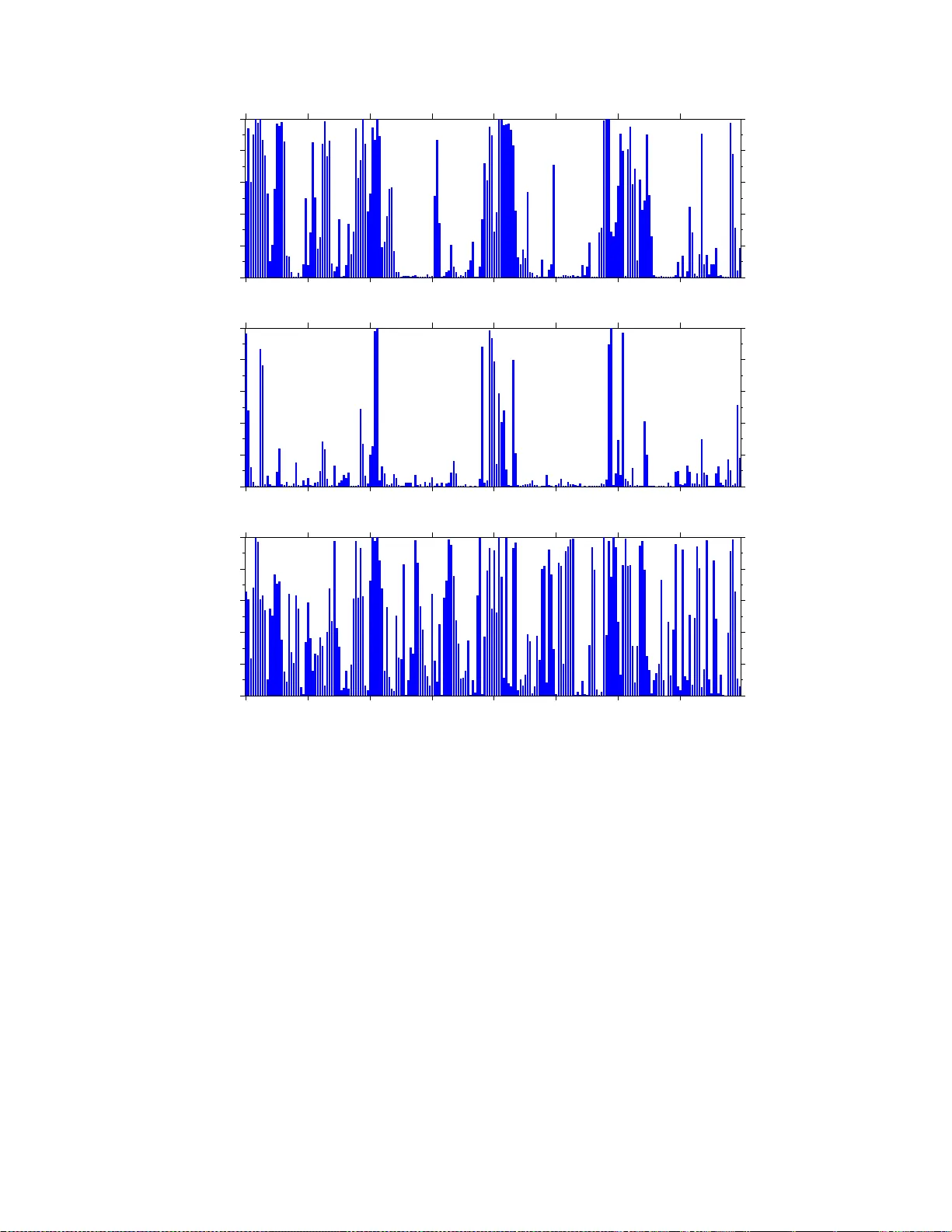
MARK O V SWITCHING MODELS: AN APPLICA TION TO R O ADW A Y SAFETY A Dissertation Submitted to the F aculty of Purdue Univ ers ity b y Nataliy a V. Malyshkina In P artial F ulﬁllmen t of the Requiremen ts for the Degree of Do ctor of Philosoph y Decem b er 20 08 Purdue Univ ersit y W est Lafay ette, Indiana ii T o my h usband Leonid and m y paren ts Nadezhda and Vla dimir iii A CKNO WLEDGMENTS First of all, I w ould lik e to thank my advisor, Professor F red Mannering. Without his in terest, encouragemen t and ﬁnancial assis tance no ne of t his researc h would be p ossible. He supp orted me during all m y three and a half y ears a t Purdue. He also ga v e me a lo t o f freedom in research . I feel ve ry luck y to b e his student. I w ould like to thank Profess or Andrew T ark o, m y co-advisor, for his v ery help- ful commen ts and encouragemen t. I am especially g r ateful t o him for the acciden t frequency data that he pr ovided fo r the study rep orted in this dissertation. In addition, I w ould lik e to thank Jos e Thomaz for preparing the accide n t sev erit y data that w as used in this study . I w ould lik e to thank Professor Kristofer Jennings and Profess or Jon F ric k er for their helpful commen ts and for c arefully reading this dissertation. I also w ould lik e to thank m y colleagues and friends for their help and supp ort during my stay on Purdue campus. Finally , I feel inﬁnite lo v e and gratitude to m y w onderful f a mily – m y h usband Leonid, m y mother Nadezhda and m y father Vladimir. I o w e ev erything I hav e to them and to their lov e and supp ort. iv T ABLE OF CONTENTS P a ge LIST OF T ABLES . . . . . . . . . . . . . . . . . . . . . . . . . . . . . . . . vi LIST OF FIGURES . . . . . . . . . . . . . . . . . . . . . . . . . . . . . . . viii LIST OF SYMBOLS . . . . . . . . . . . . . . . . . . . . . . . . . . . . . . . ix ABSTRA CT . . . . . . . . . . . . . . . . . . . . . . . . . . . . . . . . . . . x CHAPTER 1. INTR O D UCT ION . . . . . . . . . . . . . . . . . . . . . . . . 1 1.1 Motiv ation and research ob jectiv es . . . . . . . . . . . . . . . . . . 1 1.2 Organization . . . . . . . . . . . . . . . . . . . . . . . . . . . . . . 3 CHAPTER 2. LITERA TURE REVIEW . . . . . . . . . . . . . . . . . . . . 4 2.1 Acciden t frequency studies . . . . . . . . . . . . . . . . . . . . . . . 4 2.2 Acciden t sev erity studies . . . . . . . . . . . . . . . . . . . . . . . . 8 2.3 Mixed studies . . . . . . . . . . . . . . . . . . . . . . . . . . . . . . 13 CHAPTER 3. MODEL SPECIFICA TION . . . . . . . . . . . . . . . . . . . 15 3.1 Standard coun t data mo dels of acciden t frequencies . . . . . . . . . 16 3.2 Standard m ultinomial logit mo del of acciden t sev erities . . . . . . . 19 3.3 Mark ov switc hing pro cess . . . . . . . . . . . . . . . . . . . . . . . 20 3.4 Mark ov switc hing count data mo dels of a nnual acciden t frequencies . . . . . . . . . . . . . . . . . . . . . . . . . . . . . . . . 22 3.5 Mark ov switc hing count data mo dels of wee kly a cciden t frequencies . . . . . . . . . . . . . . . . . . . . . . . . . . . . . . . . 24 3.6 Mark ov switc hing multinomial logit mo dels of acciden t sev erities . . . . . . . . . . . . . . . . . . . . . . . . . . . . . . . . . 26 CHAPTER 4. MODEL ESTIMA TION AND COMP ARISON . . . . . . . . 29 4.1 Ba y esian inference and Ba y es formula . . . . . . . . . . . . . . . . . 29 4.2 Comparison of statistical mo dels . . . . . . . . . . . . . . . . . . . . 31 4.3 Mo del p erformance ev aluat io n . . . . . . . . . . . . . . . . . . . . . 32 CHAPTER 5. MARK O V CHAIN MONTE CARLO SIMULA TION METHODS . . . . . . . . . . . . . . . . . . . . . . . . . . . . . . . . . . 34 5.1 Hybrid Gibbs sampler and Metrop olis-Hasting algorithm . . . . . . 34 5.2 A general represen tation of Marko v switc hing mo dels . . . . . . . . 37 v P a ge 5.3 Choice of the prior probability distribution . . . . . . . . . . . . . . 43 5.4 MCMC simulations: step-b y-step algorithm . . . . . . . . . . . . . 47 5.5 Computational issues and o ptimiz ation . . . . . . . . . . . . . . . . 53 CHAPTER 6. FREQUENCY MOD EL ESTIMA TION RESUL TS . . . . . . 59 6.1 Mo del estimation results for annual frequency data . . . . . . . . . 59 6.2 Mo del estimation results for w eekly frequency data . . . . . . . . . 74 CHAPTER 7. SEVERITY MODEL ESTIMA TION RESUL TS . . . . . . . 89 CHAPTER 8. SUMMAR Y AND CONCLUSIONS . . . . . . . . . . . . . . 109 LIST OF REFERENCES . . . . . . . . . . . . . . . . . . . . . . . . . . . . 114 APPENDIX . . . . . . . . . . . . . . . . . . . . . . . . . . . . . . . . . . . . 1 18 VIT A . . . . . . . . . . . . . . . . . . . . . . . . . . . . . . . . . . . . . . . 122 vi LIST OF T ABLES T able P a ge 6.1 Estimation results fo r standard P oisson and negativ e binomial models of ann ual acciden t frequencies . . . . . . . . . . . . . . . . . . . . . . . . 63 6.2 Estimation results for zero-inﬂated and Mark o v switc hing P oisson mo dels of a nnual acciden t frequencies . . . . . . . . . . . . . . . . . . . . . . . 65 6.3 Estimation res ults for zero-inﬂated and Mark ov switc hing negativ e bino- mial mo dels of ann ual acciden t frequencies . . . . . . . . . . . . . . . . 67 6.4 Summary statistics of explanatory v ariables that en ter t he models of an- n ual and w eekly acciden t frequencies . . . . . . . . . . . . . . . . . . . 70 6.5 Estimation results for P o iss on mo dels of w eekly acciden t frequencies . . 78 6.6 Estimation results fo r nega t iv e binomial mo dels o f w eekly acciden t fre- quencies . . . . . . . . . . . . . . . . . . . . . . . . . . . . . . . . . . . 80 6.7 Correlations of the p o ste rior probabilities P ( s t = 1 | Y ) with w eather- condition v ariables f or the full MSNB mo del . . . . . . . . . . . . . . . 86 7.1 Estimation results for m ultinomial logit mo dels of sev erity outcomes of one-v ehicle acciden ts on Indiana interstate hig hw ay s . . . . . . . . . . . 92 7.2 Estimation results for m ultinomial logit mo dels of sev erity outcomes of one-v ehicle acciden ts on Indiana US routes . . . . . . . . . . . . . . . . 93 7.3 Estimation results for m ultinomial logit mo dels of sev erity outcomes of one-v ehicle acciden ts on Indiana state routes . . . . . . . . . . . . . . . 94 7.4 Estimation results for m ultinomial logit mo dels of sev erity outcomes of one-v ehicle acciden ts on Indiana count y roa ds . . . . . . . . . . . . . . 95 7.5 Estimation results for m ultinomial logit mo dels of sev erity outcomes of one-v ehicle acciden ts on Indiana streets . . . . . . . . . . . . . . . . . . 96 7.6 Estimation results for m ultinomial logit mo dels of sev erity outcomes of t w o -v ehicle acciden ts on Indiana streets . . . . . . . . . . . . . . . . . . 97 7.7 Explanations and summary statistics fo r v ariables and parameters listed in T ables 7.1 – 7.6 and in T ables A.1 – A.4 . . . . . . . . . . . . . . . . . 99 vii T able P a ge 7.8 Correlations of the p osterior probabilities P ( s t = 1 | Y ) with eac h other and with w eather-condition v ariables (for the MSML mo dels of acciden t sev erities) . . . . . . . . . . . . . . . . . . . . . . . . . . . . . . . . . . 106 A.1 Es timation results for mu ltinomial lo g it models of sev erity outcomes of t w o -v ehicle acciden ts on Indiana inters tate hig h w a ys . . . . . . . . . . 118 A.2 Es timation results for mu ltinomial lo g it models of sev erity outcomes of t w o -v ehicle acciden ts on Indiana US routes . . . . . . . . . . . . . . . . 11 9 A.3 Es timation results for mu ltinomial lo g it models of sev erity outcomes of t w o -v ehicle acciden ts on Indiana state routes . . . . . . . . . . . . . . . 1 2 0 A.4 Es timation results for mu ltinomial lo g it models of sev erity outcomes of t w o -v ehicle acciden ts on Indiana count y roads . . . . . . . . . . . . . . 121 viii LIST OF FIGURES Figure P a ge 5.1 Auxiliary time indexing of observ atio ns f or a general Marko v switc hing pro cess represen tation. . . . . . . . . . . . . . . . . . . . . . . . . . . 38 6.1 The histogram of 10 4 generated χ 2 v alues fo r the MSNB mo del of annual acciden t frequencies. The vertical line sho ws the observ ed v alue of χ 2 . 69 6.2 Five -y ear time series of the p osterior probabilities P ( s t,n = 1 | Y ) of the unsafe state s t,n = 1 fo r f o ur selected roa dw a y segmen ts ( t = 1 , 2 , 3 , 4 , 5). These plots are for the MSNB mo del of ann ual acciden t frequencies. . 71 6.3 Histograms o f the p osterior probabilities P ( s t,n = 1 | Y ) (the top plot ) and of the p osterior exp ectations E [ ¯ p ( n ) 1 | Y ] (the b ottom plo t ) . Here t = 1 , 2 , 3 , 4 , 5 and n = 1 , 2 , . . . , 335. These histograms are for the MSNB mo del of ann ual acciden t frequencies. . . . . . . . . . . . . . . . . . . 74 6.4 The t o p plot sho ws the we ekly acciden t frequencies in Indiana. The b ot- tom plot sho ws w eekly p osterior probabilities P ( s t = 1 | Y ) f o r the full MSNB mo del of w eekly acciden t frequencies . . . . . . . . . . . . . . . 82 7.1 W eekly p osterior probabilities P ( s t = 1 | Y ) for the MSML models esti- mated for sev erity of 1-v ehicle acciden ts on in terstate hig h w a ys (top plot) , US routes (middle plo t) and state routes (b ottom plot). . . . . . . . . 103 7.2 W eekly p osterior probabilities P ( s t = 1 | Y ) for the MSML models esti- mated for sev erit y of 1-v ehicle acciden ts o ccurring on coun t y ro ads (to p plot), streets (middle plot) and f or 2-v ehicle acciden ts o ccurring on streets (b ottom plot). . . . . . . . . . . . . . . . . . . . . . . . . . . . . . . . 104 ix LIST OF SYMBOLS AADT Av erag e Annual D aily T raﬃc AIC Ak aike Information Criterion BIC Ba y esian Information Criterion BTS Bureau of T ransp ortation Statistics i.i.d. indep ende n t and identically distributed MCMC Mark ov Chain Monte Carlo M-H Me trop olis-Hasting ML Multinomial logit MLE Maxim um Lik eliho o d Estimation MS Mark ov Switc hing MSML Mark ov Switc hing Multinomial Logit MSNB Mark ov Switc hing Negativ e Binomial MSP Mark ov Switc hing P o isson NB Negative Binomial PDO Prop ert y Damag e Only ZINB Zero-inﬂated Negativ e Binomial ZIP Zero-inﬂated P oisson x ABSTRA CT Malyshkina, Nataliy a V. Ph.D., Purdue Univ ersit y , Decem b er 2008. Mark ov Switc h- ing Mo dels: an Application to Ro a dw a y Safety . Ma jor Professors: F red L. Mannering and Andrew P . T ark o. In this researc h, t w o-state Marko v switc hing mo dels are prop osed to study acciden t frequencies and sev erities. These mo dels assume that there are t w o unobserv ed states of r o adw a y safet y , and that roadwa y en tities (e.g., roadw a y segmen ts) can switc h b et w een t hese states o v er time. The states are distinct, in the sense that in the diﬀeren t states acciden t frequencies or sev erities are generated b y separate pro cesses (e.g., P o isson, negativ e binomial, m ultinomial log it). Ba y esian inference metho ds and Mark ov Chain Mon te Carlo (MCMC) sim ulations are used for estimation of Mark o v switc hing mo dels. T o demonstrate the applicabilit y of the approach, w e conduct the follo wing three studies. In the ﬁrst study , tw o-state Mar ko v switc hing coun t data mo dels are considered as an a lternativ e to zero-inﬂated mo dels, in order to account for prep onderance of zeros t ypically observ ed in acciden t frequency data. In this study , one of the states of road- w ay safet y is a zero-acciden t stat e, whic h is p erfectly safe. The o t he r state is an un- safe state, in whic h acciden t frequencies can b e p ositiv e and are generated by a giv en coun t ing pro cess – a P oisson or a negativ e binomial. Tw o- state Mark o v switc hing P o iss on mo del, t w o-state Mark o v switc hing negativ e binomial mo del, and standard zero-inﬂated mo dels are estimated for annual acciden t frequencies o n selected Indiana in terstate high w ay segmen ts ov er a ﬁv e- year time p erio d. An imp ortant adv an tage o f Mark ov switc hing models o v er zero-inﬂated mo dels is that the former allow a direct xi statistical estimation of what states sp eciﬁc roadw ay segmen ts are in, while the later do not. In the second study , t w o -state Mark ov switc hing P oisson mo del and tw o-state Mark ov switc hing negat ive binomial mo del are estimated using wee kly acciden t fre- quencies on selected Indiana interstate highw a y segmen ts o v er a ﬁv e-y ear time p erio d. In this study , b oth states of roadw a y safet y are unsafe. Th us, acciden t frequencies can b e p ositiv e and are generated b y either P oisson or negative binomial pro cesse s in b oth states. It is found that the more frequen t state is safer and it is corr elat ed with b etter w eather conditions. The less frequen t state is found to b e less safe and to b e correlated with adv erse w eather conditions. In the third study , t w o-state Marko v switc hing multinomial logit mo dels are esti- mated for sev erit y outcomes of acciden ts o ccurring on Indiana roads ov er a fo ur-y ear time p erio d. It is aga in found that the mo r e frequen t state of roa dw a y safet y is corre- lated with b etter w eather conditions. The less frequen t state is found to b e correlated with adv erse w eather conditions. One of the most imp ortant results found in eac h of the three studies, is that in eac h case the estimated Mark ov switc hing models are strongly fa v ored by acciden t frequency and sev erit y data a nd result in a sup erior statistical ﬁt, as compared to the corresp onding standard (single-state) mo dels. 1 CHAPTER 1. INTR O D UCT ION This c hapt er explains the motiv ation and ob jectiv es o f the presen t researc h, and the organization of this dissertation. 1.1 Motiv ation and researc h ob jec tiv es According to Bureau of T ransp ortation Statistics [BTS, 2008], in 2006, 99 . 55% of all transp ortation related acciden ts ( inc luding air, railroad, transit, w aterb orne and pip eline acciden ts) w ere motor v ehicle acciden ts on r o adw a ys. Moto r v ehicle acciden ts result in f a talities, injuries and property damage, and represen t high cost not only for in v olv ed indiv iduals but also for our so ciet y as a whole. In particular, on av erage, ab out one-quarter of the costs of crash es is paid direc tly b y the party in v o lved, while the so ciet y pa ys the rest. As an example of the economic burden related to motor v ehicle crashes, in the y ear 2000 the estimated cost of acciden ts o ccurred in the United States was 23 1 billion dollars, whic h is ab out 820 dollar s p er p erson or 2 p ercen t o f the gross domestic pro duct [BTS, 2008]. These n um b ers sho w that roadwa y ve hicle tra v el safet y has an enormous imp ortance for our so ciet y and for the national economy . As a res ult, extensiv e res earc h o n roadwa y safet y is o ngoing, in order t o b etter understand the most import a n t factors t ha t con tribute to v ehicle acciden ts. In general, there are t w o measures of roadwa y safet y that ar e commonly consid- ered: 1. The ﬁrst measure ev aluates acciden t frequencies on roadw ay segmen ts. Acciden t frequency on a roa dwa y segmen t is obtained b y coun ting the n umber o f acci- 2 den ts o ccurring on t his segmen t during a sp eciﬁed p erio d of time. Then coun t data statistical mo dels (e.g. Poiss on, negativ e binomial mo dels and their zero- inﬂated coun terparts) are estimated for acciden t frequencie s o n diﬀeren t road- w ay segmen ts. The explanatory v ariables used in these mo dels are the roadwa y segmen t c haracteristics (e.g. roadwa y segmen t len gth, curv ature, slope, t yp e, pa v emen t qualit y , etc). 2. The second measure ev aluates acciden t sev erity outcomes as determined by the injury lev el sustained b y the most sev erely injured individual (if any) in v olv ed in to the acciden t. This ev aluation is done by using data o n individual acciden t s and estimating discrete outcome statistical mo dels (e.g. ordered probit and m ultinomial logit mo dels) for the acciden t sev erity outcomes. The explanatory v ariables us ed in these models are the indiv idual acciden t c haracteristics (e.g. time and lo cation o f a n acciden t, w eather conditions and roadwa y characteristic s at the acciden t lo cation, c haracteristics of the v ehicles and drivers in v olv ed, etc). These tw o measures of roadw ay safet y are complemen tary . On one hand, an acciden t frequency study pro vides a statistical mo del of the probability of an acciden t o ccurring on a roadw a y segmen t. O n the o ther hand, an acciden t sev erity study pro vides a statistical mo del of the conditional probabilit y o f a sev erit y outcome of a n acciden t, g iv en the acciden t o ccurred. The unconditional probability of the acciden t sev erity outcome is the pro duct of its conditional probability and the pro ba bilit y o f the a cc iden t. The main ob jectiv e of this researc h study is to prop ose a new statistical approa ch to mo deling acciden t frequencies and sev erities, whic h ma y provide new guidance to theorists and practitioners in the area of r oadw ay safety . Our approac h is based on application of tw o-state Mark o v switc hing mo dels of acciden t frequencies and sev eri- ties. These mo dels assume an existence of tw o unobserv ed states of roadw a y safet y . The r o adw a y en tit ies (e.g., roadwa y segmen ts) are assumed to b e able to switc h b e- t w een these states ov er time, and the switc hing pro cess is assumed to b e Mark o vian. 3 Acciden t f req uencies and sev erit y outcomes are a ss umed to b e generated b y tw o dis- tinct data-generating pro ce sses in the tw o states. Two-state Marko v switc hing mo dels a v oid sev eral drawbac ks of the popular con v en tio nal mo dels of acciden t f req uencies and sev erities. W e estimate Mark o v switc hing mo dels and compare them to the con- v entional mo dels. W e ﬁnd that the former are strongly fav ored b y acciden t frequency and sev erity data and pro vide a superio r statistical ﬁt as compared to the la t er. Be- cause of the complexity o f Marko v switc hing mo dels, this researc h emplo ys Bay esian inference and Marko v Chain Mon te Carlo (MCMC) simulations for their statistical estimation. 1.2 Org a nization An o verv iew of the previous researc h on a cc iden t f req uency and sev erity is pre- sen ted in Chapter 2. Chapter 3 giv es sp ec iﬁcation of the tw o-state Marko v switc hing and con v en t io nal mo dels that are pro p osed, considered and estimated in this study . Ba y esian inference metho ds are given in Chapter 4. Chapter 5 presen ts Mark o v Chain Mon te Carlo (MCMC) simulation tec hniques used for Ba y esian inference and mo del estimation in this study . The mo del estimation r esults for acciden t frequencies are presen ted in Chapter 6. The mo del estimation results for a cciden t sev erities are giv en in Chapter 7. Finally , we discuss our results and give conclusions in Chapter 8. Some of the results are give n in the App endix at the end. 4 CHAPTER 2 . LITERA TURE REVIEW This chapter includes a brief o v erview of t he previous roadw ay safety studies of ac- ciden t frequencies and s ev erities. First, w e giv e an o v erview of acciden t frequency studies and standard statistical mo dels used for acciden t frequencie s. Then w e re- view previous w ork on sev erities of acciden ts. Finally , we discuss studies that consider b oth acciden t frequencies and acciden t sev erities. The literature review o f this c hap- ter do es not claim to b e full or ex haustiv e. A more detailed literat ure review, a s w ell a s a comprehensiv e description of con ven tional metho dologies commonly used in roadw a y safet y studies, can b e fo und in W ashington et al. [2003]. 2.1 Acciden t frequency studies Considerable res earc h has b een conducted on understanding and predicting ac- ciden t frequencies (the n um b er of acciden ts o ccurring on r o adw a y segme n ts o v er a giv en t ime p erio d). Because acciden t frequencies are non-negative in t egers, coun t data mo dels are a reasonable statistical mo deling approac h. Simple mo deling ap- proac hes include P oisson mo dels and negativ e binomial (NB) mo dels. These mo dels assume a single pro cess for acciden t data generation (a P oisson pro cess or a negativ e binomial pro cess) and in v olve a nonlinear regression of the observ ed acciden t fre- quencies on v arious roadwa y-segmen t c haracteristics (suc h as roadwa y geometric and en vironmental factors). Selec ted previous researc h on acciden t frequencies, conducted b y application of coun t data mo dels, is as follow s: • Hadi et al. [199 5 ] used negativ e binomial mo dels to estimate the eﬀect of cross section roadwa y design elemen ts (e.g. presence o f curb, lane width) a nd tra ﬃc 5 v o lume on acciden t frequencies for diﬀeren t types of highw a ys. The authors found that some cross section design elemen ts can inﬂuence acciden t ra tes (e.g. lane width, in terc ha ng e presence, sp eed limit) and that some o ther do not hav e an y eﬀect on num b er of acciden ts (e.g. t yp e of friction course material). • Shank ar et al. [19 95] applied a negativ e binomial mo del to a n accide n t dat a col- lected in W ashington State. Roadw ay geometries of ﬁxed-equal length ro a dw a y segmen ts (e.g. horizon ta l and v ertical a lig nme n ts), w eather, and other seasonal eﬀects w ere analyzed alo ng with o v erall acciden t frequencies of sp eciﬁc acciden t t yp es (e.g., rear-end and same direction acciden ts). This researc h concluded that hig h w a y segmen ts with c hallenging geometries as w ell as areas that fre- quen tly experience adv erse w eather conditions are imp ortan t determinan ts of acciden t frequency . • P o c h a nd Mannering [1996] estimated a negative binomial regression of the fre- quencies of acciden t s a t intersec tion approa c hes in Seattle suburban areas. The authors of t his pap er considered traﬃc v olume, geometric characteristics o f in- tersection approac hes (e.g. approach sight-distance, sp eed limit) and approac h signalization c hara cteris tics (e.g. eigh t- phase signal) a s the mo del explanatory v ariables. Authors found a signiﬁcan t inﬂuence o f s ome of these v ariables on acciden t f req uencies at intersec tion approac hes. In particular, t hey found that high left-turn and opp osite traﬃc v olumes considerably increase num b ers o f acciden ts at in t ers ection approac hes. • Miaou and Lord [2 003], ba se d on acciden t da t a collected in T oron to, examined generally a cc epted statistical mo dels (P oisson and NB) applied to acciden t fre- quencies in tersections. By using the empirical Bay es metho d, mathematical prop erties a nd p erformance of diﬀeren t p opular model functional forms were considered. The autho rs questioned in v ariability of the disp ersion parameter, giv en the complexit y of the traﬃc in teraction in an in tersection area. In addi- 6 tion, the full Bay es statistical a pproac h w as used f or model speciﬁcation a nd estimation. • P ark and Lord [2008] rec en tly conside red ﬁnite mixture P oisson and negativ e binomial mo dels of acciden t frequencies, in order to accoun t for heterogenous p opulations of acciden t da ta. Acciden t data heterog eneity can result from data gene ration b y distinct (Poisson or NB) pro cesses that op erate in diﬀer- en t unobserv ed states of ro a dw a y safet y . P ark and Lord [2008] suggested a t w o -component ﬁnite mixture negativ e binomia l mo del as the b est mo del to accoun t for acciden t data heterogeneit y in their data sample. • Recen tly , Anastasop oulos and Mannering [2008] applied random parameters coun t models to the analysis of acciden t frequ encies. The authors found these mo dels to b e b eneﬁcial for acciden t frequency prediction. Random parame- ter mo dels can p oten t ially deﬁne unique parameters for eac h roadw ay segmen t, but t hese mo dels still a s sume a single state for eac h segmen t. This single- state assumption would a ls o b e true for coun t mo dels with rando m eﬀects [see Shank ar et al., 19 9 8 ]. • Anastasop oulos et al. [2 008] w ere the ﬁrst to use t obit regression mo dels for prediction of acciden t rates (accide n t rates are n um b er of acciden ts happ ened p er unit roadw a y segmen t length and p er unit a v eraged annual daily traﬃc v o lume). They considered ﬁv e-y ear acciden t data a nd fo und t ha t in ternational roughness index (of the pav emen t) , pa v emen t rutting, the pa v emen t’s condition rating, median types and width, shoulder widths, n um b er of ramps and bridges, horizon tal and vertical curv es, rumble strips, a nn ual av erage da ily tra ve l and the p ercen t o f com bination truc k in the traﬃc stream ha v e a signiﬁcan t impact on acciden t rates. Because a prep onderance of zero-a cciden t o bserv ations is often observ ed in empir- ical dat a , some researc hers hav e applied zero-inﬂa t ed P oisson (ZIP) and zero-inﬂated negativ e binomial (Z INB) models fo r predicting acciden t f r eq uencies. Zero-inﬂat ed 7 mo dels assume a t wo-state pro ces s fo r acciden t data generation. One state is a ss umed to b e p erfectly safe with zero a cc iden ts (o v er the duration of time b eing considered). The other state is assumed to b e unsafe with a p ossibilit y of nonzero acciden t frequen- cies in whic h acciden t s can happen and acciden t frequencie s are generated b y some giv en coun ting pro cess (P o iss on or negativ e binomial). Be low are selected studies that are based o n an application of zero- inﬂated coun t data mo dels: • Miaou [1 994] applied Poiss on regression, zero- inﬂat ed P oisson (Z IP ) regression, and NB regression to determine a relationship b et wee n geometric design c ha r - acteristics of roadw a y segmen ts and the n um b er o f truc k acciden ts. Results suggest that under the maxim um lik eliho o d estimation (MLE) metho d, all three mo dels p erform similarly in terms of estimated truc k-inv olv ed acciden t frequencies across roadw a y segmen ts. T o mo del the relationship, the author recommended the use of a P oisson regression as an initial mo del, then the use of a negativ e binomial mo del if the acciden t frequency data is o v erdisp erse d, and the use of a zero-inﬂated Poiss on mo del if the data con tains an excess of zero observ ations. • Shank ar et al. [1 9 97] studied the distinction b et w een safe and unsafe roadw a y segmen ts b y estimating zero-inﬂated P o isson and zero-inﬂated negativ e binomial mo dels for acciden t frequenc ies in W ashington State. The a uthors established the underlying principles of zero-inﬂated models, ba se d on a t wo-state data- generating pro cess for acciden t frequencies . The t w o states ar e a safe stat e that corresp onds to the zero acciden t lik eliho o d on a roadw ay segmen t, and a n unsafe state. The results sho w that t wo-state zero-inﬂated structure mo dels pro vide a sup erior statistical ﬁt to acciden t frequency data as compared to the con- v entional single-state mo dels (without zero-inﬂation). Th us, the authors found that zero- inﬂa t ed mo dels are helpful in rev ealing and understanding imp ortan t factors that a ﬀec t acciden t frequencies with prep onderance of zeros. 8 • Lord et al. [200 5 , 2007] addressed the question of c ho osing the b est a pproac h to the mo deling of ro a dw a y acciden t data b y using count data mo dels (e.g. whether to use standard single-state or zero-inﬂated models). Authors a r g ued that an application of zero- inﬂa t ed mo dels to t he analysis of acciden t data with a prep onderance of ze ros is not a defensible mo deling appro ac h. They argued that an excess of zeros can be caus ed by an inappropriate data collection and b y man y other f a ctors, instead of due to a t w o- states pro cess. In addition, they claimed that it is unreasonable to expect some roadw ay segmen ts to b e alw a ys p erfectly safe and questioned “safe” and “unsafe” state deﬁnitions. The authors also argued that zero- inﬂated mo dels do not explicitly acc ount fo r a lik ely po ss ibilit y for r o adw a y segmen ts to change in time fr o m o ne state to another. Lord et al. [2005, 2007] concluded that , while an application of zero- inﬂated models often provides a better statistical ﬁt to an observ ed acciden t frequency data, the a pplicability of these mo dels can b e questioned. 2.2 Acciden t sev erit y studies Researc h eﬀorts in predicting acciden t sev erit y , suc h as prop erty damag e, injury and fat alit y , are clearly v ery imp ortant. In the past there ha s b een a la r g e num b er of studies that fo cused o n mo deling acciden t sev erit y outcomes. The proba bilities of sev erity outcomes of an accide n t are conditio ned on the o ccu rrence of t he acciden t. Common mo deling approac hes of acciden t sev erity include m ultinomial logit mo dels, nested logit mo dels, mixed logit mo dels a nd ordered pro bit mo dels. All acciden t sev erity mo dels in v o lve nonlinear regression of the observ ed a cc iden t sev erity out- comes on v ario us acciden t c haracteristics and related factors (suc h as roadw ay and driv er c haracteristics, environme n tal factors, etc). Some of the past acciden t sev erity studies are a s follow s: 9 • O’Donnell and Connor [1996] explored sev erity of motor v ehicle acciden ts in Australia by estimating the parameters of ordered multiple c hoice mo dels: o r - dered logit and probit mo dels. By studying driv er, passengers and v ehicle char- acteristics (e.g. v ehicle ty p e, seating po sition of ve hicle o ccupan ts, blo o d alcohol lev el of a drive r), the authors found the eﬀects o f these c haracteristics on the probabilities of diﬀeren t t yp es o f sev erit y outcomes. F or example, they found that the older the victims are and t he higher the ve hicle sp eeds are, the higher the pr o babilities of serious injuries and deaths are. • Shank ar and Mannering [1996] estimated the lik eliho o ds of motorcycle rider ac- ciden t sev erity outcomes. In their researc h w ork, a multinomial logit mo del w as applied to a 5-year W ashington state data fo r single-v ehicle motorcycle colli- sions. It w as found that a helmeted-riding is an eﬀectiv e means of reduc ing injury sev erit y in an y types of collisions, except in ﬁxed-ob j ec t collis ions. A t the same time, alcoho l- impaired riding, high age of a mot orcyc le rider, ejection of a rider, w et pa v ement, interstate as a ro a dw a y type, sp eedin g and rider inat- ten t io n w ere fo und to b e the facto r s that increase roadw a y motorcycle acciden t sev erity . • Shank ar et al. [1996] used a neste d logit mo del fo r statistical analysis of acci- den t sev erit y outcomes on rural high wa ys in W ashington State. They found that en vironment conditions, high w a y design, acciden t ty p e, drive r and veh icle char- acteristics s igniﬁcan tly inﬂuence acc iden t sev erit y . The y found that o v erturn acciden ts, r ear - end acciden ts on w et pa v emen t, ﬁxed-ob ject acciden ts, and fa il- ure to use the restraint b elt system lead to higher probabilities of injury or/and fatality acciden t outcomes, while icy pav emen t and single-ve hicle collisions lead to higher probabilit y of prop ert y damag e o nly outcomes. • Duncan et al. [1998] applied an ordered probit mo del to injury sev erity out- comes in truc k-passenger car rear-end collisions in North Carolina. They found 10 that injury sev erit y is increased by darknes s, high sp eed diﬀeren tia ls, high speed limits, w et grades, drunk driving, and b eing female. • Chang and Mannering [1 999] fo cused on the eﬀects of truc ks and v ehicle o ccu- pancies on acciden t sev erities. They estimated nested logit m o dels for s ev er- it y outcomes of truck -inv olv ed and non-tr uck-in v olv ed acciden ts in W ashington State a nd found that acciden t injury sev erity is noticeably w orsened if the ac- ciden t has a truc k in v olv ed, and that the eﬀects of truc ks a r e more signiﬁcant for multi-o ccupan t ve hicles than for single-o ccupan t v ehicles. • Khattak [200 1 ] estimated ordered probit mo dels for sev erit y outcomes o f multi- v ehicle rear-end acciden ts in North Carolina. In particular, the results of his researc h indicate that in t w o-v ehicle collisions the leading drive r is more lik ely to b e sev erely injured, in three-v ehicle collisions the driv er in the middle is mor e lik ely to b e sev erely injured, and b eing in a new er vehic le protects the driv er in rear-end collisions. • Ulfarsson [2001], Ulfarsson and Mannering [2004] fo cus ed on male and female diﬀerences fo r acciden t sev erity outcomes. They used m ultinomial lo git mo dels and acciden t data from W ashington Sta te. They found signiﬁcan t behavioral and ph ysiological diﬀerences b et we en genders, a nd also found tha t probability of fa tal and disabling injuries is higher f or females as compared t o males. • Ko c kelm an a nd Kw eon [2002] applied o rdere d pro bit mo dels to mo deling of driv er injury sev erit y out comes. They used a nation wide acciden t data sample and found that pic kups and sp ort utilit y v ehicles are less ( mo r e) safe than passenger cars in single-ve hicle ( tw o-vehic le) collisions. • Khattak et al. [2002] fo cused on the safet y o f a ged drivers in the United States. Nine-y ear Iow a-statewide acciden t data w as considered and the ordered probit mo deling tec hnique w as implem en ted for acciden t sev erit y modeling. Authors insp ec ted v ehicle, roadw ay , driver, collision, and en vironmen ta l c haracteristics 11 as factors that may potentially eﬀect acciden t sev erity of aged driv ers. The mo deling results we re consisten t with a common sense, for example, an animal- related acciden t tends to ha v e sev ere consequences fo r e lderly drive rs. Also, it w as found that acciden t s with farm v ehicles in v olved are highly sev ere fo r elderly driv ers in Iow a. • Ab del-A ty [2003] used ordered pro bit mo dels for analysis of driv er injury sev er- it y outcomes at diﬀerent roa d lo cations (roa dw a y segmen ts, signalized in tersec- tions, toll plazas) in Cen tral Florida. He found highe r proba bilities of sev ere acciden t outcomes for o lder drivers, male drivers , those not wearing seat b elt, driv ers who sp eed, those who drov e v ehicles struc k at the driv er’s s ide, those who driv e in rural areas, and drive rs using electronic toll collection device (E- P a ss ) at toll plazas. • Y ama mo t o and Shank ar [2004] applied biv ariate ordered probit mo dels to an analysis of drive r’s and passenger’s injury sev erities in collisions with ﬁxed ob- jects. They considered a 4 - y ear acciden t data sample from W ashington State and f o und that collisions with leading ends of guardrail and trees tend to cause more sev ere injuries, while collisions with sign p osts, fa ce s of guardrail, concrete barrier or bridge and fences tend to cause less sev ere inj uries. They also found that prop er use of veh icle restraint system strongly decreases the probabilit y of sev ere injuries and fa talities. • Khorashadi et al. [2005] ex plored the diﬀerences of driv er injury sev erities in rural and urban a cciden ts inv olving large truc ks. Using four y ears of California acciden t data and multinomial logit mo del approach, they found cons iderable diﬀerences betw een rural and urban acciden t injury s ev erities. In particular, they found that the probability of sev ere/fatal injury increases by 26 % in rural areas and b y 70 0 % in urban areas when a tractor-tr ailer combination is in volv ed, as opposed to a single-unit truck b eing in v olv ed. They also found t hat in ac- 12 ciden ts whe re alcohol o r drug use is iden tiﬁed, the probabilit y of sev ere/fatal injury is increased b y 250 % and 800% in rural a nd urban areas resp ectiv ely . • Islam and Mannering [20 06 ] studied driv er ag ing and its eﬀect on male and female single-v ehicle a cc iden t injuries in Indiana. They employ ed m ultinomial logit mo dels and found signiﬁcan t diﬀerences b et w een diﬀeren t g end ers and age groups. Speciﬁcally , they found an increase in probabilities of fatality for y o ung and middle-aged male driv ers when they hav e pa ssengers, an increase in probabilities of injury for middle-aged female drivers in v ehicles 6 y ears old or older, a nd an increase in fatality probabilities for males older tha n 65 y ears old. • Malyshkina [2006], Malyshkina and Mannering [2006] fo cused on t he relation- ship b et w een sp eed limits and roa dw a y safet y . Their researc h explored t he inﬂuence o f the p osted sp eed limit on the causation and sev erity of acciden ts. Multinomial logit statistical mo dels were estimated fo r causation and sev erity outcomes of diﬀerent t yp es of acciden ts on diﬀeren t road classes. The results sho wed that sp eed limits do not hav e a statistically s igniﬁcan t adv erse eﬀect on unsafe-sp eed-related causation of acciden ts on all roads. At the same time higher sp eed limits generally increase the sev erit y of acciden ts on the ma jority of ro ads o ther than inters tate high w a ys (on in terstates sp eed limits w ere found to ha v e statistically insigniﬁcan t eﬀect on acciden t sev erity). • Sa v olainen [2006], Sa volainen and Mannering [2007] fo cu sed on the imp ortan t topic of motorcycle safety o n Indiana ro a ds . They used m ultino mial a nd nested logit mo dels and found that p o or visibilit y , unsafe sp eed, alcoho l use, not we ar- ing a helmet, right-angle and head-on collisions, and collisions with ﬁxed ob j ects increase sev erit y of motorcycle-in v o lv ed acciden ts. • Milton et al. [200 8 ], b y using acciden t sev erit y data fro m W ashington Sta te, estimated a mixed logit mo del with random parameters. This approac h allo ws estimated mo del parameters to v ary randomly across roadw a y segmen ts t o ac- coun t for unobserv ed eﬀects that can b e related to o ther factors inﬂuencing 13 roadw a y safety . Authors found t ha t, on o ne ha nd, some roa dwa y characteristic parameters (e.g. pa v emen t friction, n umber of horizon tal curv es) can b e tak en as ﬁxed. On the other hand, other mo del parameters, suc h as we ather eﬀects and volume -related mo del parameters (e.g. truck p erce n tage, av erage ann ual sno wfa ll) , are r a ndom and normally-distributed. • Eluru and Bhat [20 07] mo deled a seat b elt use endogeneit y t o acciden t sev erit y due to unsafe driving habits of drivers not using seat belts. F or sev erit y out- comes, the authors considered a system of tw o mixed probit mo dels with random co eﬃcie n ts estimated join tly for seat b elt use dummy and sev erity outcomes. The probit mo dels included random v ariables that mo derate the inﬂuence of the primary explanatory a ttributes asso ciated with driv ers. The estimation results highligh t the importance of moderatio n eﬀects, seat belt use endogeneity and the r elation of b et we en failure to use seat b elt and unsafe driving habits. 2.3 Mixed studies Sev eral pre vious researc h studies considered mo deling of b oth acciden t freq uen- cies and acciden t sev erit y outcomes. It is b eneﬁcial to look at b oth frequencies and sev erities sim ultaneously because, as men tioned ab o v e, an unconditional probability of the a cc iden t sev erity outcome is the pro duct of its conditional proba bility and the acciden t probabilit y . Sev eral mixed studies, w hic h consider both acciden t frequency and sev erity , are as follows. • Carson and Mannering [20 0 1 ] studied the eﬀect of ice w arning signs o n ice- acciden t f r equencies a nd sev erities in W ashington State. The y mo deled acciden t frequencies a nd sev erities b y using zero-inﬂated negative binomial and logit mo dels resp ectiv ely . They found that the presence of ice w arning signs w as not a signiﬁcan t factor in reducing ice-acciden t fr eq uencies a nd sev erities. 14 • Lee a nd Mannering [2002] estimated zero-inﬂated count-data mo dels and nested logit mo dels for frequencies and sev erities of run-o ﬀ-roadw ay acciden ts in W ash- ington State. They found that run-oﬀ - roadw ay acciden t frequencies can b e re- duced by a v oiding cut side slop es, decreasing (increasing) the distance from outside shoulder edge to g ua rdrail (light p oles), and decreasing the num b er of isolated trees along roadw ay . The results of their researc h also sho w that run-oﬀ-roa dwa y acciden t sev erit y is increased b y alcohol impaired driving, high sp ee ds, and the presence of a g uardrail. • Kw eon and Ko c k elman [20 0 3 ] studied probabilities of acciden ts and acciden t sev erity outcomes for a giv en ﬁxed driv er ex p osure (deﬁned as the total mile s driv en). They used P oisson and ordered probit mo dels, and cons idered a na- tion wide acciden t data sample. After normalization of acciden t rates b y driv er exp o sure , the results of their study indicated that young driv ers are far more crash prone than other drive rs, a nd that sp ort utility v ehicles and pic kups a r e more lik ely to b e in v olv ed into rollov er acciden ts. 15 CHAPTER 3 . MODEL SPECIFICA TION In this c hapter we sp ecify the statistic al models that a r e us ed a nd es timated in the presen t study . F irst, w e consider standard (conv en tional) mo dels commonly used in accide n t studies. These a re coun t data models for acciden t frequencies (P oisson, negativ e binomial mo dels and their zero-inﬂated coun terparts) and discrete outcome mo dels for acciden t sev erit y outcomes (m ultinomial logit models). Then w e explain Mark ov pro cess for the state of roa dwa y safet y . Finally , w e presen t t w o -state Mark o v switc hing mo dels for acciden t frequencies a nd sev erities. In each of the t w o states the data is gene rated b y a standard pro cess (suc h as a P oisson or a negativ e binomial in the case of accide n t frequencie s, and a m ultinomial logit in the case of acciden t sev erities). O ur presen t a tion of Marko v switc hing mo dels is similar to that o f Mark ov switc hing autoregressiv e models in econometrics [McCullo c h and Tsay, 1994, Tsay, 2002]. All statistical mo dels that we consider here, either fo r acciden t frequencies or for sev erity outcomes, are parametric and can b e fully sp eciﬁed b y a lik eliho o d function f ( Y | Θ , M ), whic h is the conditio na l probability distribution of the v ector of all observ at io ns Y , given t he vec tor of all parameters Θ of mo del M . If acciden t ev en t s are assumed t o b e indep end en t, the lik eliho o d function is f ( Y | Θ , M ) = T Y t =1 N t Y n =1 P ( Y t,n | Θ , M ) . (3.1) Here, Y t,n is the n th observ at io n during time p erio d t , and P ( Y t,n | Θ , M ) is the prob- abilit y (likelihoo d) of Y t,n . The v ector of observ ations Y = { Y t,n } includes all obser- v ations n = 1 , 2 , ..., N t o v er all time perio ds t = 1 , 2 , ..., T . Number N t is the total n um b er of observ atio ns during time p erio d t , and T is the total n um b er of time p e- rio ds. In t he case of acciden t frequencies , observ ation Y t,n is the num b er of a cc iden ts 16 observ ed on the n th roadw a y segmen t during time p erio d t (note that N t is the n um- b er of roadw ay s egmen ts in this case). In the case of acciden t sev erity , obse rv ation Y t,n is the observ ed outcome of the n th acciden t o ccurred during time p erio d t (no t e that N t is the n um b er of acciden ts in this case). V ector Θ is the v ector of a ll un- kno wn mo del parameters to b e estimated from a cc iden t data Y . W e will sp ecify the parameter ve ctor Θ separately for eac h statistical model presen ted below. Finally , mo del M = { M , X t,n } includes t he mo del’s name M (e.g. M = “negative binomial” or M = “m ultinomial logit”) and the v ector X t,n of all c haracteristic attributes (i.e. v alues of all explanatory v ariables in the mo del) tha t are a sso ciated with the n th observ at io n during time p erio d t . 3.1 Standar d coun t data mo dels o f acciden t frequencies The most p opular coun t data mo dels used for predicting acciden t frequencies are P o iss on a nd negative binomial (NB) mo dels [W ashingto n et al., 2003]. These mo dels are usually estimated b y the maxim um lik eliho o d estimation (MLE) metho d, whic h is based on t he ma ximization of the mo del like liho o d function f ( Y | Θ , M ) o v er the v alues of t he mo del estimable parameters Θ . Let the num b er o f acciden ts observ ed on the n th roadw a y segmen t during time p erio d t b e A t,n . Th us, our observ ations are Y t,n = A t,n , where n = 1 , 2 , ..., N t and t = 1 , 2 , ..., T . Here N t is the n um b er of roadw ay segmen ts observ ed during time p erio d t , and T is the total n um b er o f t ime p erio ds. The lik eliho o d function f or the P o iss on mo del of acciden t frequencies is sp ec iﬁed by equation (3.1) and the follo wing equations [W ashingto n et al., 20 03]: P ( Y t,n | Θ , M ) = P ( A t,n | Θ , M ) = P ( A t,n | β ) , (3.2) P ( A t,n | β ) = λ A t,n t,n A t,n ! exp( − λ t,n ) , (3.3) λ t,n = exp( β ′ X t,n ) , t = 1 , 2 , ..., T , n = 1 , 2 , ..., N t . (3.4) 17 Here, λ t,n is the P oisson acciden t rate for the n th roadw a y segmen t, this rate is equal to the a v erage (mean) acciden t frequency on this segmen t ov er the time p erio d t . The v a r iance of a P oisson-distributed acciden t freq uency is the same as its av erage and is equal to λ t,n . P arameter v ector β consists of unknow n mo del parameters to b e estimated. Prime means transp ose, so β ′ is the transp ose of β . In the P oisson mo del the v ector of all mo del para meters is Θ = β . V ector X t,n includes character- istic v ariables for the n th roadw a y segmen t during time p erio d t . F o r example, X t,n ma y include segmen t length, curv e c hara cteris tics, grades, and pav emen t pro p erties. Henceforth, the ﬁrst comp onen t of v ector X t,n is c ho sen to b e unity , and, therefore, the ﬁr st comp onen t of v ector β is the in tercept. The like liho o d function fo r the nega t ive binomial (NB) mo del o f acciden t frequen- cies is sp eciﬁe d by equation (3.1) and the follo wing equations [W ashington et al., 2003]: P ( Y t,n | Θ , M ) = P ( A t,n | Θ , M ) = N B ( A t,n | β , α ) , (3.5) N B ( A t,n | β , α ) = Γ( A t,n + 1 /α ) Γ(1 /α ) A t,n !  1 1 + αλ t,n  1 /α  αλ t,n 1 + αλ t,n  A t,n , (3.6) λ t,n = exp( β ′ X t,n ) , t = 1 , 2 , ..., T , n = 1 , 2 , ..., N t . (3.7) Here, Γ( ) is the standard gamma function. The o ver-dispersion parameter α ≥ 0 is an unkno wn model parameter t o b e estimated tog ethe r with ve ctor β . Th us, the v ector of all estimable parameters is Θ = [ β ′ , α ] ′ . The a v erage acciden t rate is equal to λ t,n , whic h is the same as in the case of the P oisson model. The v ariance of the acciden t rate is λ t,n (1 + αλ t,n ), whic h is higher than in the case of the Pois son mo del (if α > 0). The negativ e binomial mo del reduces to the P oisson model in the limit α → 0. In addition to the P o iss on and negative binomial mo dels, w e also consider t he stan- dard zero-inﬂat ed P oisson (ZIP) and zero-inﬂat ed negativ e binomial (Z INB) mo dels. These models accoun t for a p ossibilit y o f existence of t w o separate data-generating states: a normal count state and a zero-acciden t state. The norma l state is unsafe, and acciden ts can o ccur in it. The zero-acciden t state is p erfectly safe with no acciden ts 18 o ccurring in it. 1 Zero-inﬂated mo dels are usually used when there is a prep onderance of zeros in the data . In the case of acciden t frequency data with man y zeros in it, the probabilit y of A t,n acciden ts o ccurring on t he n th roadw a y segmen t at time pe- rio d t can b e w ell modeled b y a ZIP pro cess o r , if the data are ov er-disp erse d, b y a ZINB pro cess. The lik eliho o d functions of the Z IP and ZINB mo dels are sp eciﬁed b y equation (3.1) and the following equations [W ashington et al., 2003]: P ( Y t,n | Θ , M ) = P ( A t,n | Θ , M ) = q t,n I ( A t,n ) + (1 − q t,n ) P ( A t,n | β ) for Z IP , (3.8) P ( Y t,n | Θ , M ) = P ( A t,n | Θ , M ) = q t,n I ( A t,n ) + (1 − q t,n ) N B ( A t,n | β , α ) for Z INB , (3.9) where I ( A t,n ) = { 1 if A t,n = 0, and 0 if A t,n > 0 } , (3.10) q t,n = 1 1 + e − τ log λ t,n , (3.11) q t,n = 1 1 + e − γ ′ X t,n . (3.12) Here w e use t w o diﬀeren t sp ec iﬁcations f o r the probabilit y q t,n that the n th road- w ay segmen t is in the zero-acciden t state during time p erio d t . Scalar λ t,n is the acciden t r a te that is deﬁne d b y equation (3.4). Probabilit y distribution I ( A t,n ) is the probability mass function that reﬂects the fact that accide n ts nev er happen in the zero-acciden t state. The righ t - hand-side of equation (3.8) is a mixture of the zero-acciden t distribution I ( A t,n ) and the P oisson distribution P ( A t,n | β ) giv en by equation (3.3). The right-hand-side of equation (3.9) is a mixture of I ( A t,n ) and the negativ e bino mia l distribution N B ( A t,n | β , α ) g iv en by equation (3.6). Scalar τ and v ector γ are estimable mo del par a mete rs. W e call “Z IP- τ ” and “Z INB- τ ” the mo dels sp ec iﬁed b y equations ( 3 .8 )-(3.1 1). W e call “ZIP- γ ” and “ZINB- γ ” the mo dels sp ec- iﬁed b y equations (3.8)-(3.10) and (3.12). The ve ctor of all estimable parameters is 1 Note tha t roadway segments a re not required to stay in a particular sta te all the time and can mov e from normal count state to z e ro-accident s tate and v ic e versa. 19 Θ = [ β ′ , τ ] ′ for the ZIP- τ mo del, Θ = [ β ′ , α, τ ] ′ for the ZINB- τ mo del, Θ = [ β ′ , γ ′ ] ′ for the Z IP - γ mo del, and Θ = [ β ′ , α, γ ′ ] ′ for the Z INB- γ mo del. It is imp ortant t o note that q t,n dep ends on the estimable mo del parameters and giv es the probability of b eing in the zero-acciden t state, but q t,n is no t an estimable parameter b y itself. 3.2 Standar d multinomial logit mo del of acciden t sev erities The sev erit y outcome of an acciden t is determine d b y the injury lev el sustained b y the most se v erely injured individual (if an y) in v olv ed into the acciden t. Thus , acciden t sev erities are a discrete outcome data. Most common statistical mo del used for predicting sev erit y outcomes a re the multinomial log it mo del and the ordered probit mo del. Ho w ev er, there are tw o p oten tial problems with applying o r dered probabilit y mo dels to a cciden t sev erit y outcomes [Sav olainen and Mannering, 2007]. The ﬁrst problem is due t o under-rep orting of non-injury a cc iden ts b ecause they are less lik ely to b e rep orted to authorities. This under-rep orting can result in biased a nd inconsisten t mo del co eﬃcien t estimates in an o rdered probabilit y mo del. In contrast, the co eﬃcien t estimates of a n unordered m ultinomial logit mo del are consisten t except for the in tercept terms [W ashington et al., 2003]. The second problem is related to undesirable restrictions t hat ordered probability m o dels place o n inﬂuences of the explanatory v ar iables [W ashington et al., 200 3 ]. As a result, in this study w e consider only m ultinomia l logit mo dels fo r acciden t sev erity . Let t here b e I discrete outcomes observ ed for acciden t sev erit y (for example, I = 3 a nd these outcomes a re fa t alit y , injury and prop ert y damage only). Also let us in tro duce acciden t sev erity outcome dummies δ ( i ) t,n that are eq ual to unit y if the i th sev erity outcome is observ ed in the n th acciden t that o ccurs during time p erio d t , and to zero otherwise. Then, our indiv idual observ ations are the sev erity outcome dummies, Y t,n = { δ ( i ) t,n } , where i = 1 , 2 , ..., I . No t e that n = 1 , 2 , ..., N t and t = 1 , 2 , ..., T , whe re N t is the n um b er of acciden ts observ ed during time p erio d t , and T is the total n um b er of time p erio ds. The v ector of all observ a tions Y = { δ ( i ) t,n } 20 includes all o utcomes observ ed in all acciden ts that o ccur during a ll time p eriods. The lik eliho o d f unc tion for the m ultinomial logit (ML) mo del of acciden t sev erity outcomes is sp eciﬁed by equation (3.1) and the follo wing equations [W ashington et al., 200 3 ]: P ( Y t,n | Θ , M ) = I Y i =1 [ P ( i | Θ , M )] δ ( i ) t,n = I Y i =1 [ ML ( i | β )] δ ( i ) t,n , (3.13) ML ( i | β ) = exp( β ′ i X t,n ) P I j =1 exp( β ′ j X t,n ) , i = 1 , 2 , ..., I . (3.14) P a rameter v ectors β i consist of unkno wn mo del parameters to b e estimated, and β = { β i } , where i = 1 , 2 , ..., I . V ector X t,n con tains all c haracteristic v ariables f or the n th acciden t that o ccurs during time p erio d t . F or example, X t,n ma y include w eather and en vironmen t conditions, v ehicle and driv er characteristics , r o adw a y and pa v emen t prop erties. W e set the ﬁrst comp onen t of X t,n to unit y , a nd, therefore, the ﬁrst comp onen ts of ve ctors β i ( i = 1 , 2 , ..., I ) are the in tercepts. In addition, without loss of generalit y , w e set all β -parameters for the last sev erity outcome to zero, β I = 0 . This can b e done without loss of generalit y b ecause X t,n are assumed to b e indep enden t of the outcome i , and, therefore, the numerator and denominator in equation (3.14) can b e m ultiplied by the an arbitrary common factor [W ashington et al., 200 3]. 3.3 Mark o v switc hing pro cess Let there be N roa dw a y se gmen ts (or, more generally , roadwa y en tities or/and geographical areas) that w e observ e during s uccessiv e time p erio ds t = 1 , 2 , ..., T . 2 Mark ov switc hing mo dels, whic h will b e introduced b elo w, assume that there is an unobserv ed (laten t) state v ariable s t,n that determine s the state of roadw ay safet y for the n th roadw a y segmen t (or roadw ay e n tity , or geographical area) during time p erio d t . W e assume that the stat e v ariable s t,n can ta ke on only tw o v alues: s t,n = 0 corresp onds to the ﬁrst state, and s t,n = 1 corresp onds to the second state. The c hoice 2 In a more ge ne r al case, w e ca n observe a v a r iable n um b er of roadway segments ov er successive time per iods. Her e, for simplicit y of the pre sen ta tion, we do not consider this genera l case. How ever, our analysis is straightforw ard to extend to it. 21 of lab els “0” and “1” for the t w o states is a r bit r a ry and is a matter of con v enience. W e further assume that, for each ro adw a y segmen t n the state v aria ble s t,n follo ws a stationary t w o-state Mark ov chain pro cess in time. 3 The Mark o v prop erty means that the probability distribution of s t +1 ,n dep ends only on the v alue s t,n at time t , but not on the previous history s t − 1 ,n , s t − 2 ,n , ... [Breiman, 1 9 69]. The stationary t w o- state Marko v chain pro ce ss { s t,n } can b e speciﬁed by time-indep ende n t transition probabilities as P ( s t +1 ,n = 1 | s t,n = 0) = p ( n ) 0 → 1 , P ( s t +1 ,n = 0 | s t,n = 1) = p ( n ) 1 → 0 , (3.15) where n = 1 , 2 , ..., N . In this equation, for example , P ( s t +1 ,n = 1 | s t,n = 0) is the conditional probability of s t +1 ,n = 1 at time t + 1, giv en that s t,n = 0 at time t . Note that P ( s t +1 ,n = 0 | s t,n = 0) = p ( n ) 0 → 0 = 1 − p ( n ) 0 → 1 and P ( s t +1 ,n = 1 | s t,n = 1) = p ( n ) 1 → 1 = 1 − p ( n ) 1 → 0 . T ransition probabilities p ( n ) 0 → 1 and p ( n ) 1 → 0 are unkno wn parameters to b e e stimated from acciden t data ( n = 1 , 2 , ..., N ). The stationary unconditional probabilities of states s t,n = 0 and s t,n = 1 are 4 ¯ p ( n ) 0 = p ( n ) 1 → 0 / ( p ( n ) 0 → 1 + p ( n ) 1 → 0 ) for state s t,n = 0 , ¯ p ( n ) 1 = p ( n ) 0 → 1 / ( p ( n ) 0 → 1 + p ( n ) 1 → 0 ) for state s t,n = 1 . (3.16) It is notew orth y that the case when (for eac h roadw a y segmen t n ) the states s t,n are indep enden t and iden tically distributed in time t is a sp ecial case o f the Marko v c ha in pro cess. Indeed, this case corresp onds to histor y- indep enden t pro babilities of stat es “0” and “1 ”, therefore, p ( n ) 0 → 0 ≡ p ( n ) 1 → 0 and p ( n ) 0 → 1 ≡ p ( n ) 1 → 1 . Th us, we hav e p ( n ) 0 → 0 = p ( n ) 1 → 0 = ¯ p ( n ) 0 and p ( n ) 0 → 1 = p ( n ) 1 → 1 = ¯ p ( n ) 1 , where the last equalities in these t w o form ulas follow from equations (3.16). 3 Stationarity of { s t,n } is in the statis tica l sense [Breiman, 1969]. 4 These can b e found from the following stationarity co nditions: ¯ p ( n ) 0 = [1 − p ( n ) 0 → 1 ] ¯ p ( n ) 0 + p ( n ) 1 → 0 ¯ p ( n ) 1 , ¯ p ( n ) 1 = p ( n ) 0 → 1 ¯ p ( n ) 0 + [1 − p ( n ) 1 → 0 ] ¯ p ( n ) 1 and ¯ p ( n ) 0 + ¯ p ( n ) 1 = 1 [Breiman, 1969]. 22 3.4 Mark o v switc hing count data mo dels of a nnual acciden t frequencies When considering ann ual acciden t frequency data b elo w, w e will use and estimate t w o -state Mark o v switc hing P oisson (MSP) a nd tw o-state Mark o v switc hing negative binomial ( MS NB) mo dels that are prop osed as follow. Similar to zero-inﬂated mo d- els, these ann ual-acciden t-frequency Mark ov switc hing mo dels assume that one of the t w o states o f ro a dw a y safety is a zero-acciden t state, in whic h acciden t s nev er happ en. The other state is assumed to b e an unsafe state with p ossibly non-zero acciden ts o c- curring. MSP and MSNB mo dels resp ectiv ely assume P oisson and negativ e binomial (NB) da t a -generating pro cesse s in the unsafe state. Without loss of generalit y , b elo w w e tak e s t,n = 0 to b e t he zero-acciden t state and s t,n = 1 to b e t he unsafe state. As in the case of the standa r d coun t data mo dels of acciden t fr equencies (see Section 3.1 ) , in this section, a single observ ation is the nu m b er of acciden ts A t,n that o ccur on the n th roadw a y segmen t during time p erio d t . There are T time p erio ds, each is equal to a year, and the p erio ds are t = 1 , 2 , ..., T . F or simplicity of presen tation, we assume that the n umber o f roadw ay segmen ts is constan t ov er time 5 , N t = N = const, and, therefore, the segmen t s are n = 1 , 2 , ..., N . The ve ctor of a ll observ at io ns Y = { Y t,n } = { A t,n } includes all acciden t frequencies A t,n ( t = 1 , 2 , ..., T and n = 1 , 2 , ..., N ). F or eac h r o adw a y segmen t n , the s tate s t,n can change ev ery y ear. The lik eliho o d functions of t he tw o-state Mark ov switc hing Poisson (MSP) and t w o -state Mark o v switc hing negativ e binomial (MSNB) mo dels of an nual a cc iden t frequencies A t,n are sp eciﬁed by eq uation (3 .1) with N t = N , and by the follo wing equations: P ( Y t,n | Θ , M ) = P ( A t,n | Θ , M ) =    I ( A t,n ) if s t,n = 0 P ( A t,n | β ) if s t,n = 1 (3.17) 5 The analys is is e asily extended to the case when we observe a v a riable n umber o f roadwa y seg men ts N t 6 = cons t during time p erio ds t , see also foo tnote 2 on pa ge 20. In this cas e it would b e con venien t to count all se g men ts as n = 1 , 2 , ..., N and to count the time p erio ds as t = T ( n ) i , T ( n ) i + 1 , ..., T ( n ) f , where the n th segment is assumed to b e observed during interv a l T ( n ) i ≤ t ≤ T ( n ) f of successive time per iods. 23 for t he MSP mo del of ann ual acciden t frequencies , and P ( Y t,n | Θ , M ) = P ( A t,n | Θ , M ) =    I ( A t,n ) if s t,n = 0 N B ( A t,n | β , α ) if s t,n = 1 (3.18) for the MS NB model of ann ual acciden t frequencie s. Here zero-acciden t probabilit y distribution I ( A t,n ), giv en b y equation (3.10 ), reﬂects the fact that accid en ts nev er happ en in t he zero-acciden t state s t,n = 0. Probability distributions P ( A t,n | β ) and N B ( A t,n | β , α ) a re the standard P oisson and negativ e binomial probability mass func- tions, see equations (3.3) and (3.6) resp ectiv ely . V ector β is the v ector of estimable mo del parameters and α is the negat ive binomial o v er- dispersion par amete r. T o en- sure that α is non-negativ e, during mo del estimation w e consider its lo g arithm instead of it. F or each ro a dw a y segmen t n the state v ariable s t,n follo ws a stationary t w o-state Mark ov c hain pro cess as described in Section 3.3. Because the state v a r ia bles s t,n are unobserv a ble, the v ector of all estimable pa- rameters Θ mus t include all states ( s t,n ), in a ddition to all model parameters ( β -s, α -s) and all transition probabilities ( p ( n ) 0 → 1 , p ( n ) 1 → 0 ). Th us, Θ = [ β ′ , α, p (1) 0 → 1 , ..., p ( N ) 0 → 1 , p (1) 1 → 0 , ..., p ( N ) 1 → 0 , S ′ ] ′ , (3.19) where v ector S = [( s 1 , 1 , ..., s T , 1 ) , ..., ( s 1 ,N , ..., s T ,N )] ′ con tains all state v a lues s t,n and has length T × N . Of course, in the case of the MSP mo del, o v er-disp ersion parameter α do es not en ter equation (3.19). Note that, if p ( n ) 0 → 1 < p ( n ) 1 → 0 , then, according to equations (3 .16), w e ha v e ¯ p ( n ) 0 > ¯ p ( n ) 1 , and, on a v erage, for the n th roadw a y se gmen t state s t,n = 0 o ccurs more frequen tly than state s t,n = 1. On the other hand, if p ( n ) 0 → 1 > p ( n ) 1 → 0 , then state s t,n = 1 o ccurs more frequen tly for the n th segmen t. In addition, note that here the c hoice of a y ear as the length of the time p eriods t = 1 , 2 , ..., T is arbitrary . F o r example, one can consider quarterly ( or other) p erio ds instead. Finally , it is imp ortan t to understand that although the MSP and MSNB mo dels giv en by Equations (3 .1 7) and (3.18) assume state s t,n = 0 to be perfectly safe a nd 24 zero-acciden t, this state can b e (and probably should b e) view ed as an appro ximation for nearly safe states, in whic h acciden ts ra rely o ccur. 6 3.5 Mark o v switc hing count data mo dels of wee kly a cciden t f r eq uencies When considering w eekly acciden t frequency data b elo w, w e will use and estimate t w o -state Mark o v switc hing P oisson (MSP) a nd tw o-state Mark o v switc hing negative binomial (MSNB) mo dels that are prop osed as f o llo ws. In eac h of the tw o states ( s t,n = 0 and s t,n = 1) thes e w eekly-acciden t-frequency mo dels assume a standard P o iss on data-g enerating pro cess deﬁned b y equation (3.3), or a standard negativ e binomial pro cess deﬁned b y equation (3.6) . Th us, b oth states are assumed to b e unsafe f or these mo dels. W e observ e the num b er of acciden ts A t,n that o ccur on the n th roadw a y segmen t during time p erio d t , whic h is a we ek in t his case. Let there b e T we ekly time p erio ds in total. Let us again assume that the n umber of roa dw a y segmen ts is constan t o v er time, N t = N = const (see fo otnote 5 on page 2 2 ). Th us, in equation (3.1) the v ector of a ll observ a tions is Y = { Y t,n } = { A t,n } , where t = 1 , 2 , ..., T and n = 1 , 2 , ..., N . In addition, for w eekly-acciden t-frequency Mark ov switc hing mo dels, w e assume that a ll ro adw a y segmen ts alw a ys hav e the same state, a nd, therefore, the state v a r ia ble s t,n = s t dep ends on t ime p erio d t only . This is b ecause, here, state s t is inte nded to capture common unobserv ed factors inﬂuencing roadw a y s afety on all segmen ts. Corresp ondingly , all roadwa y segmen ts switc h b et w een the states with the same transition pro babilities p ( n ) 0 → 1 = p 0 → 1 and p ( n ) 1 → 0 = p 1 → 0 . With this, the lik eliho o d functions for the t w o-state Mark o v switc hing P oisson (MSP) a nd tw o-state Mark ov switc hing negativ e binomial ( MSNB) mo dels of we ekly 6 Nearly safe states hav e average accident rates λ t,n ≪ 1 [see Equa tions (3 .4) and (3.7)]. In this case, the per fectly safe, zer o-accident state, which has λ t,n = 0, serves as a go od approximation for these nearly safe states. 25 acciden t frequencies A t,n are sp eciﬁed by equation (3.1) with N t = N , and by the follo wing equations: P ( Y t,n | Θ , M ) = P ( A t,n | Θ , M ) =    P ( A t,n | β (0) ) if s t = 0 P ( A t,n | β (1) ) if s t = 1 (3.20) for t he MSP mo del of w eekly a cc iden t frequencies, and P ( Y t,n | Θ , M ) = P ( A t,n | Θ , M ) =    N B ( A t,n | β (0) , α (0) ) if s t = 0 N B ( A t,n | β (1) , α (1) ) if s t = 1 (3.21) for the MSN B mo del of w eekly acciden t frequencie s. Here, t = 1 , 2 , ..., T and n = 1 , 2 , ..., N . P robability distributions P ( . . . ) and N B ( . . . ) are the s tandard Poiss on and negativ e binomial probability mass functions, see equations (3.3) and (3.6) re- sp ec tiv ely . P a rameter v ectors β (0) and β (1) , and negative binomial ov er-disp ersion parameters α (0) ≥ 0 and α (1) ≥ 0 a r e the unknow n estimable mo del parameters in the t wo stat es s t = 0 and s t = 1. T o ensure that α (0) and α (1) are non-negativ e, their loga rithms are considere d during mo del estimation. Because, we c ho ose the ﬁrst comp onen t of X t,n to b e equal to unit y , the ﬁrs t comp onen ts of β (0) and β (1) are the in tercepts in the tw o states. Note that the state v ariable s t follo ws a station- ary t w o-state Mark ov chain pro cess with transition probabilities p 0 → 1 and p 1 → 0 as described in Section 3.3. Because t he state v ariables s t are unobserv able, the v ector of all estimable param- eters Θ m ust include all states ( s t ), in addition to all mo del parameters ( β -s, α -s) and all transition probabilities ( p 0 → 1 , p 1 → 0 ). Th us, Θ = [ β ′ (0) , α (0) , β ′ (1) , α (1) , p 0 → 1 , p 1 → 0 , S ′ ] ′ . (3.22) where vec tor S = [ s 1 , ..., s T ] ′ has length T a nd contains all state v alues. In the case of the MSP mo del, ov er-disp ersion parameters α (0) and α (1) are absen t from equation (3.22). 26 Without loss of generalit y , w e assume tha t (on av erage) state s t = 0 o ccurs more or equally frequen tly tha n state s t = 1. Therefore, ¯ p 0 ≥ ¯ p 1 , and from Equations (3.16) w e obtain restriction 7 p 0 → 1 ≤ p 1 → 0 . (3.23) In this case, w e can refer to states s t = 0 and s t = 1 as “mo r e frequen t” a nd “less frequen t” states resp ectiv ely . Note that here the c ho ice of a wee k a s the length of the time p erio ds t = 1 , 2 , ..., T is arbitrary . F or example, one can consider daily (or other) p erio ds instead. 3.6 Marko v switc hing mu ltinomial logit mo dels of acciden t sev erities When considering acciden t sev erit y data b elo w, w e will use and estimate t w o- state Mark o v switch ing multinomial logit (MSML) mo del that is prop osed as follow s. In eac h of the tw o states (0 and 1), this mo del assumes standard m ultino mia l logit (ML) data-generating pro cess that is deﬁned by equation (3.14) and described in Section 3 .2. W e observ e sev erity outcome dummies δ ( i ) t,n that a r e equal to unit y if the i th sev erity outcome is o bse rv ed in the n th acciden t that o ccurs during time p erio d t , and to zero otherwise. W e conside r we ekly time p erio ds, t = 1 , 2 , ..., T , where T is the total num b er of p erio ds observ ed. Then, the vector of all observ ations Y = { δ ( i ) t,n } includes all o utcome s observ ed in all accide n ts that o ccur during all time p erio ds, i = 1 , 2 , ..., I , n = 1 , 2 , ..., N t and t = 1 , 2 , ..., T . Here I is the total n um b er of p ossible sev erit y outcomes, and N t is the n um b er of acciden ts observ ed during w eekly time perio d t . F or MSML mo dels of acciden t sev erities, w e again ass ume that all roadw a y segmen ts (where acciden ts happ en) alwa ys ha v e the same state of roadw ay safet y , and, therefore, the state v ariable s t,n = s t dep ends on time p erio d t only (in this case, state s t captures common unobserv ed factors that inﬂuence safety on a ll 7 Restriction (3.2 3) is introduced for the purp ose of av o iding the problem of switc hing of state lab els, 0 ↔ 1. This problem w ould otherwise arise b ecause of the s ymmetry of the likeliho od functions given by equations (3.1), (3.20) and (3 .2 1) under the la bel switching. 27 segmen ts). Corresp ondingly , all roadw a y segmen ts switc h b et w een the states with the same transition probabilities p ( n ) 0 → 1 = p 0 → 1 and p ( n ) 1 → 0 = p 1 → 0 . The lik eliho o d function for the tw o-state Mark ov switc hing m ultinomial logit (MSML) mo del of accid en t sev erit y outcomes is sp eciﬁed by equation (3.1) and the follo wing equations: P ( Y t,n | Θ , M ) = I Y i =1 [ P ( i | Θ , M )] δ ( i ) t,n =        I Q i =1  ML ( i | β (0) )  δ ( i ) t,n if s t = 0 I Q i =1  ML ( i | β (1) )  δ ( i ) t,n if s t = 1 , (3.24) where n = 1 , 2 , ..., N t and t = 1 , 2 , ..., T . Probabilit y distributions ML ( i | β (0) ) and ML ( i | β (1) ) are the standard m ultinomial log it proba bility mass functions in the t w o states, see equation (3.14). Here β (0) = { β (0) ,i } and β (1) = { β (1) ,i } , where i = 1 , 2 , ..., I . P ara me ter v ectors β (0) ,i and β (1) ,i are unknown estimable mo del parameters in states 0 and 1 resp ectiv ely . Since we choose the ﬁrst comp onen t of X t,n to b e equal to unity , the ﬁrst comp onen ts o f v ectors β (0) ,i and β (1) ,i are the interce pts. Similar to the case of the standard (single-state) ML mo del presen ted in Section 3.2, here, w e set all β -parameters for t he last sev erity outcome to zero, β (0) ,I = β (1) ,I = 0 . The v ector of a ll estimable parameters Θ includes all states ( s t ), in addition t o all mo del parameters ( β -s) and all transition probabilities ( p 0 → 1 , p 1 → 0 ). Th us, Θ = [ β ′ (0) , β ′ (1) , p 0 → 1 , p 1 → 0 , S ′ ] ′ . (3.25) where v ector S = [ s 1 , ..., s T ] ′ has length T and con ta ins all state v alues. In analogy with the assumption made in the previous section, here, without loss of generalit y , w e assume that (on av erage) state s t = 0 o ccurs more or equally frequen tly than state s t = 1. Therefore, ¯ p 0 ≥ ¯ p 1 , and from equations ( 3 .16) w e again obtain restriction p 0 → 1 ≤ p 1 → 0 . (3.26) 28 In this case, w e can refer to states s t = 0 and s t = 1 as “mo r e frequen t” a nd “less frequen t” states resp ectiv ely . Note that here the c ho ice of a wee k a s the length of the time p erio ds t = 1 , 2 , ..., T is arbitrary . F or example, one can consider daily (or other) p erio ds instead. 29 CHAPTER 4 . MODEL ESTIMA TION AND COMP ARISON This c ha pter presen ts t he basics of Bay esian estimation of standard mo dels and Mark ov switc hing mo dels o f acciden t frequencies and sev erities. W e also discuss com- parison o f diﬀeren t mo dels b y using Ba y esian a pproac h, and an ev aluatio n of mo del ﬁt p erformance. 4.1 Bay esian inference and Ba y es formula Statistical estimation of Marko v switc hing mo dels is complicated b y unobserv abil- it y of the state v ariables s t,n (or s t ). 1 As a result, the traditional maxim um lik eliho o d estimation (MLE) pro cedure is of very limited use for Mark ov switc hing mo dels. Instead, a Ba y esian inferen ce approac h is used. Giv en a model M with lik eliho o d function f ( Y | Θ , M ), the Bay es formula is f ( Θ | Y , M ) = f ( Y , Θ |M ) f ( Y |M ) = f ( Y | Θ , M ) π ( Θ |M ) R f ( Y , Θ |M ) d Θ . (4.1) Here f ( Θ | Y , M ) is the p osterior probabilit y distribution of mo del parameters Θ conditional on the observ ed data Y a nd mo del M . F unction f ( Y , Θ |M ) is the join t probabilit y distribution of Y and Θ given mo del M . F unction f ( Y |M ) is the marginal lik eliho o d function – the probability distribution of da ta Y giv en mo del M . F unction π ( Θ |M ) is the prior probabilit y distribution of parameters tha t reﬂects prior kno wledge ab out Θ . The intuition b ehind equation (4.1) is straig h tforward: g iven mo del M , the p osterior distribution accoun ts for bo th the observ a tions Y and our 1 F or exa mple, in the case of Markov switching mo dels of weekly accide nt frequencies, we will hav e 260 time perio ds ( T = 2 6 0 weeks of av ailable data). In this case, there are 2 260 po ssible combinations for v alue of vector S = [ s 1 , ..., s T ] ′ . 30 prior kno wledge of Θ . W e use the harmonic mean form ula to calculate the marginal lik eliho o d f ( Y |M ) of data Y [see Kass and Raftery, 1 9 95] as, f ( Y |M ) − 1 = f ( Y | M ) − 1 Z π ( Θ |M ) d Θ = f ( Y |M ) − 1 Z f ( Θ , Y |M ) f ( Y | Θ , M ) d Θ = f ( Y | M ) − 1 Z f ( Θ | Y , M ) f ( Y |M ) f ( Y | Θ , M ) d Θ = Z f ( Θ | Y , M ) f ( Y | Θ , M ) d Θ = E  f ( Y | Θ , M ) − 1   Y  , (4.2) where E ( . . . | Y ) is the p o ste rior expectation (which is calculated by using the p o ste rior distribution). In our study (and in most practical studie s), the direct application of equa- tion (4.1) is not feas ible b ecause the parameter vector Θ con tains to o man y com- p onen ts, making in tegr a tion o v er Θ in equation (4.1) extremely diﬃcult (see fo ot- note 1 o n pag e 29). Ho w ev er, the p osterior distribution f ( Θ | Y , M ) in equation (4.1) is kno wn up to its normalization constan t, namely f ( Θ | Y , M ) ∝ f ( Y , Θ |M ) = f ( Y | Θ , M ) π ( Θ |M ). As a result, w e use Marko v Chain Monte Carlo (MCMC) sim- ulations, whic h pro vide a con v enien t and pra ctical computational metho do logy for sampling from a probability distribution kn ow n up to a constan t (the p osterior dis- tribution in our case). Giv en a la r ge enough p osterior sample o f parameter v ector Θ , an y p osterior expectation and v a r iance can b e found and Ba y esian inference can b e readily applied. In the next c hapter w e describ e our c ho ice of prior distribution π ( Θ |M ) and the MCMC sim ulations in detail. The prior distribution is c hosen to b e wide and essen tially noninformat ive. F or the MCMC sim ulatio ns , w e wrote a sp ecial n umerical co de in t he MA TLAB programming lang ua ge and tested it (for details see the next c hapter). In the end of this section, let us make a short noteworth y dig r ession. In Ba y esian statistics mo del observ ations and mo del par a mete rs are treated on an equal fo oting. Therefore, fo r Mark o v switc hing mo dels, one c an treat the ve ctor of all state v alues S as latent mo del parameters, or as latent (hidden) o bse rv ations. W e treat S as mo del parameters. As a result, in our approac h, the transition probabilities p ( n ) 1 − > 0 and p ( n ) 0 − > 1 do not en ter the lik eliho o d function f ( Y | Θ , M ), whic h is a function of 31 S and mo del co eﬃcien ts ( β - s, α -s, γ -s, τ ) only (refer to the lik eliho o d functions presen ted in the previous chapter). In this case, the Mark o v switc hing prop erty is treated as a prior information, and the prior distribution, given in the next chapter, reﬂects this prop erty (in other words, we a prior i sp ecify that the state v ariable s t,n follo ws a Mark o v pro cess in time). If w e treated state v alues S as laten t observ ations, then the vec tor of all observ a tion w ould include b oth Y and S . In this case, the lik eliho o d function w ould dep end on the transition probabilities and w ould b ecome f ( Y , S | Θ \ S , M ) = f ( Y | Θ , M ) f ( S | Θ \ S , M ), where Θ \ S means all c omp onen t s of Θ except S . In any case, for the purp ose of mo del comparison discussed b elo w, the marginal like liho o d should alw a ys b e deﬁned as f ( Y |M ) [not as f ( Y , S |M )] b ecaus e Y is the only data that is truly observ ed. 4.2 Comparison of statistical mo dels F or comparison of diﬀeren t mo dels w e use the following Bay esian appro ac h. Let there b e tw o mo dels M 1 and M 2 with parameter v ectors Θ 1 and Θ 2 resp ec tiv ely . Assuming that we ha v e equal preferences of these mo dels, their prior probabilities are π ( M 1 ) = π ( M 2 ) = 1 / 2. In this case, the ratio of the mo dels’ p osterior probabilities, P ( M 1 | Y ) and P ( M 2 | Y ), is equal to the Bay es factor. The later is deﬁned as the ratio of the mo dels’ marginal lik eliho o ds [Kass and Raftery, 1995]. Th us, w e ha v e P ( M 2 | Y ) P ( M 1 | Y ) = f ( M 2 , Y ) /f ( Y ) f ( M 1 , Y ) /f ( Y ) = f ( Y |M 2 ) π ( M 2 ) f ( Y |M 1 ) π ( M 1 ) = f ( Y |M 2 ) f ( Y |M 1 ) , (4.3) where f ( M 1 , Y ) and f ( M 2 , Y ) ar e the join t distributions of the mo dels and the data, f ( Y ) is t he unconditional distribution of the data, and the marginal lik eliho o ds f ( Y |M 1 ) and f ( Y |M 2 ) are giv en b y equation (4.2). If the ratio in equation ( 4.3) is larger than one, then mo del M 2 is fav ored, if the ratio is less than one, then model M 1 is fa v ored. An adv a n tage o f the use of Bay es factors is that it ha s an inheren t p enalt y for including to o many parameters in the mo del and guards against o v erﬁtting. 2 2 There are other frequently used mo del co mparison cr iter ia, for example, the deviance information criterion, DIC = 2 E [ D ( Θ ) | Y ] − D ( E [ Θ | Y ]), where deviance D ( Θ ) ≡ − 2 ln[ f ( Y | Θ , M )] [Rob ert, 32 4.3 Mo del p erformance ev aluation T o ev aluate the p erformance of mo del {M , Θ } in ﬁtting the observ ed data Y , w e carry out a χ 2 go o dness -of- ﬁt test [Maher and Summersgill , 1996, Co w an , 1998, W o o d, 20 02, Press et a l., 2007]. In the case of acciden t frequency mo dels, quan tity χ 2 is 3 χ 2 = T X t =1 N t X n =1 [ Y t,n − E ( Y t,n | Θ , M )] 2 v ar ( Y t,n | Θ , M ) , (4.4) where E ( Y t,n | Θ , M ) and v ar ( Y t,n | Θ , M ) a r e the exp ectations and v aria nce s of the observ at io ns Y t,n . In acciden t frequency studies, the observ ations are the frequencies, Y t,n = A t,n on roadw ay segmen t n during time p erio d t . F or example, from equa- tions (3.6) , (3.7) and (3.21) fo r the MSNB mo del of w eekly acc iden t frequenc ies w e ﬁnd the followin g form ulas for the (unconditional o f state) expectations and v a riances : E ( Y t,n | Θ , M ) = ¯ p 0 λ (0) t,n + ¯ p 1 λ (1) t,n and v ar ( Y t,n | Θ , M ) = ¯ p 0 λ (0) t,n (1 + α (0) λ (0) t,n ) + ¯ p 1 λ (1) t,n (1 + α (1) λ (1) t,n ) + ¯ p 0 ¯ p 1 ( λ (1) t,n − λ (0) t,n ) 2 , where λ (0) t,n = exp( β ′ (0) X t,n ) and λ (1) t,n = exp( β ′ (1) X t,n ) are the mean acciden t rates in the states s t = 0 and s t = 1 resp ectiv ely . F or the MSNB mo del of ann ua l acciden t frequencies one needs to set λ (0) t,n ≡ 0 in t hese formulas b e- cause state s t = 0 is the zero-acciden t state in this case. The appropriate fo r m ulas for P oisson mo dels can be obtained by setting the o v er-disp ersion parameters ( α -s) to zero. In the limit o f asymptotically normal distribution of large acciden t frequenc ies, χ 2 has the c hi-square distribution with degrees of freedom equal to the n um b er o f observ at io ns min us the n um b er of mo del par a mete rs [W o o d, 2002]. Because w eekly (and eve n ann ual) a cc iden t frequencies are t ypically small, in this study , w e do not rely o n the assumption of their asymptotic norma lity . Instead, w e carry out Mon te 2001]. Mo dels with smaller DIC a r e fav ored to mo dels with larg er DIC. How ever, DIC is theoreti- cally base d on the assumption of asymptotic multiv ar iate normality of the p osterior distribution, in which case DIC reduces to AIC [Spiegelha lter et al., 2002]. As a result, we prefer to rely on a math- ematically rigorous and formal Bay es facto r appro ac h to mo del selection, as given by equation (4.3). 3 Note that for a standar d Poisson distribution, the v a r iances are equal to the means , v ar ( Y t,n | Θ , M ) = E ( Y t,n | Θ , M ), a nd equation (4.4) reduces to the Pearson’s χ 2 . 33 Carlo sim ulations to ﬁnd the distribution of χ 2 [Co w an , 1998]. This is done b y generating a large num b er of a rtiﬁcial data sets under the h yp othesis that the mo del {M , Θ } is true, computing and recording the χ 2 v alue for eac h data set, and then using these v alues to ﬁnd the distribution of χ 2 . This distribution is t hen used to ﬁnd the go o dness-of-ﬁt p- v a lue, equal to the probability that χ 2 exceeds the observ ed v alue of χ 2 (the later is calculated by using the observ ed data Y ). 4 In the case of acciden t sev erity mo dels, we use the P earson’s χ 2 , deﬁned as χ 2 = T X t =1 N t X n =1 I X i =1 [ δ ( i ) t,n − P ( i | Θ , M )] 2 P ( i | Θ , M ) , (4.5) where the a cciden t sev erity outcome dummies δ ( i ) t,n are equal to unit y if t he i th sev erity outcome is observ ed in the n th acciden t tha t o ccurs during time p erio d t , and to zero otherwise. According to equation (3.24), the theoretical unconditional probability of the i th outcome is P ( i | Θ , M ) = ¯ p 0 ML ( i | β (0) ) + ¯ p 1 ML ( i | β (1) ). 4 Note that for this Mo nte Carlo simulations approach, spe c iﬁc a tion of quantit y χ 2 is actually very ﬂexible. F or exa mple, one can p otentially use [ Y t,n − E ( Y t,n | Θ , M )] 4 /v ar ( Y t,n | Θ , M ) 2 under the sum in equa tio n (4.4) for the go o dnes s-of-ﬁt test. How ever, in this ca se χ 2 would not b ecome c hi-squar e distributed even in the a symptotic limit of large accident frequencies. 34 CHAPTER 5. MARK O V CHAIN MONTE CARLO SIMULA TION METHODS W e use MCMC sim ula tions for Ba y esian inference and mo del estimation. This ch ap- ter presen ts MCMC simulation metho ds in detail. Fir s t, w e describe a h ybrid Gibbs sampler and the Metropolis-Hasting algorithm. Next, w e explain a general M ark ov switc hing mo del represen tation that we use for all Mark o v switc hing mo dels of acci- den t frequencies and sev erities. After that w e describ e our c hoice of prior probability distribution. Then w e g iv e detailed step-by-ste p algorithm used fo r our MCMC sim- ulations. F inally , in the end of this c hapter, w e brieﬂy o v erview sev eral imp ortant computational issue s and optimizations that allo w us to mak e Bay esian-MCMC es- timation reliable, e ﬃcien t and n umerically acc urate. F or brevity , in this c hapter w e omit mo del sp eciﬁcation notation M in all equations. F o r example, in this chapter w e write the p osterior distribution f ( Θ | Y , M ) simply as f ( Θ | Y ), and etc. 5.1 Hybrid Gibbs sampler and Metrop olis-Hasting algo rithm As w e ha v e mentioned in the previous chapter, b ecause the p osterior distribution, giv en b y the Bay es formula (4.1), is extremely diﬃcult to ﬁnd exactly , but is relativ ely easy to ﬁnd with accuracy up to its normalization constant, w e use Mark o v Chain Mon te Carlo (MCMC) simulations. They provide a feasible statistical me tho dology for sampling from a n y probability distribution known up t o a constan t, the p osterior distribution in our case. T o obtain draws of t he para mete rs v ector Θ from a p osterior distribution f ( Θ | Y ), w e use the hy brid Gibbs sampler, whic h is an MCMC sim ulation algo rithm tha t 35 in v o lves b oth Gibbs and Metropo lis -Hasting sampling [McCullo c h and Tsa y, 1994, Tsa y , 2 0 02, SAS Institute Inc., 2 006]. Assume that Θ is comp osed o f K comp onen ts: Θ = [ θ ′ 1 , θ ′ 2 , ..., θ ′ K ] ′ , whe re θ k can b e scalars or vec tors, k = 1 , 2 , ..., K . Then , the h ybrid Gibbs sampler w orks as follow s: 1. Cho ose an a rbitrary initial v a lue of the parameter v ector, Θ = Θ (0) , suc h tha t f ( Θ (0) | Y ) > 0 [i.e. f ( Θ (0) | Y ) ∝ f ( Y , Θ (0) ) = f ( Y | Θ (0) ) π ( Θ (0) ) > 0]. 2. F or eac h g = 1 , 2 , 3 , . . . , parameter v ector Θ ( g ) is generated comp onen t - b y- comp onen t f r o m Θ ( g − 1) b y the follo wing pro cedure: (a) First, draw θ ( g ) 1 from the conditional p osterior probability distribution f ( θ ( g ) 1 | Y , θ ( g − 1) 2 , ..., θ ( g − 1) K ). If this distribution is exactly kno wn in a closed analytical form, then w e draw θ ( g ) 1 directly from it. This is G ibbs sampling. If the conditional posterior dis tribution is know n up to an unk now n nor- malization constant, then w e dra w θ ( g ) 1 b y using the Metrop olis-Hasting (M-H) alg orithm describ ed b elow . This is M-H sampling. (b) Second, fo r all k = 2 , 3 , ..., K − 1, draw θ ( g ) k from the conditional p osterior distribution f ( θ ( g ) k | Y , θ ( g ) 1 , ..., θ ( g ) k − 1 , θ ( g − 1) k +1 , ..., θ ( g − 1) K ) by using either Gibbs sampling (if the distribution is kno wn exactly) or M-H sampling (if the distribution is kno wn up to a constan t). (c) Finally , dra w θ ( g ) K from the conditional po ste rior probability distribution f ( θ ( g ) K | Y , θ ( g ) 1 , ..., θ ( g ) K − 1 ) b y using either G ibbs or M- H sampling. 3. The resulting Mark o v c hain { Θ ( g ) } con v erges to the true p osterior distribution f ( Θ | Y ) as g → ∞ . Note that all conditional p osterior distributions are prop ortional to the join t distri- bution f ( Y , Θ ) = f ( Y | Θ ) π ( Θ ). F or example, we ha v e f ( θ k | Y , θ 1 , ..., θ k − 1 , θ k +1 , ..., θ K ) = f ( Y , θ 1 , ..., θ k − 1 , θ k , θ k +1 , ..., θ K ) f ( Y , θ 1 , ..., θ k − 1 , θ k +1 , ..., θ K ) ∝ f ( Y , θ 1 , ..., θ k − 1 , θ k , θ k +1 , ..., θ K ) = f ( Y , Θ ) . (5 .1 ) 36 By using the h ybrid Gibbs sampler algorithm describ ed ab o v e, w e obtain a Marko v c ha in { Θ ( g ) } , where g = 1 , 2 , . . . , G bi , G bi + 1 , . . . , G . W e discard the ﬁrst G bi “burn- in” draws b ecause they can dep end on the initial choice Θ (0) . Of the remaining G − G bi dra ws, w e ty pically store ev ery third or ev ery tenth dra w in the compu ter memory . W e use t hese dra ws fo r Bay esian inference. W e typically c ho ose G ranging from 3 × 10 5 to 3 × 1 0 6 , and G bi = G/ 10. In our study , a single MCMC sim ulation run tak es fro m o ne day to couple w eeks on a single computer CPU. W e usually use eigh t diﬀeren t c hoices of the initial parameter v ector Θ (0) . Th us, we obtain eigh t Mark ov c ha ins of Θ , and use them for the Bro oks-Gelman-Rubin diagnostic of con v erg ence of our MCMC sim ulat io ns [Bro oks and Gelman, 1998], for details see Section 5.5 b elo w. W e also c heck con ve rgence b y monitoring the lik eliho o d f ( Y | Θ ( g ) ) and the join t distribution f ( Y , Θ ( g ) ). W e use the Metrop olis-Hasting (M-H) algorithm to sample from conditio nal p os- terior distributions know n up to their normalization constan ts. 1 Sp eciﬁc ally , our goal here is to dra w θ ( g ) k from f ( θ k | Y , θ ( g ) 1 , ..., θ ( g ) k − 1 , θ ( g − 1) k +1 , ..., θ ( g − 1) K ) distribution that is not known exactly , so w e cannot use the Gibbs sampling. The M-H a lg orithm w o rks as follo ws: • Cho ose a jumping probability distribution J ( ˆ θ k | θ k ) of ˆ θ k . It m ust stay the same for all draws g = G bi + 1 , ..., G , and w e discuss its choice b elo w. • Draw a candidate ˆ θ k from J ( ˆ θ k | θ ( g − 1) k ). • Calculate ratio ˆ p = f ( ˆ θ k | Y , θ ( g ) 1 , . . . , θ ( g ) k − 1 , θ ( g − 1) k +1 , . . . , θ ( g − 1) K ) f ( θ ( g − 1) k | Y , θ ( g ) 1 , ..., θ ( g ) k − 1 , θ ( g − 1) k +1 , ..., θ ( g − 1) K ) × J ( θ ( g − 1) k | ˆ θ k ) J ( ˆ θ k | θ ( g − 1) k ) . (5.2) • Set θ ( g ) k =    ˆ θ k with pro babilit y min( ˆ p, 1 ) , θ ( g − 1) k otherwise . (5.3) 1 In general, the M-H a lgorithm allows to make draws from any proba bilit y distribution known up to a c o nstan t. The algor ithm co n verges as the num b er of draws go es to inﬁnity . 37 Note that the unknow n normalization constant of f ( . . . ) cancels out in equation (5.2). Also, if the jumping distribution is symmetric J ( ˆ θ k | θ k ) = J ( θ k | ˆ θ k ), then the ratio J ( θ ( g − 1) k | ˆ θ k )  J ( ˆ θ k | θ ( g − 1) k ) b ecomes equal to unit y and Metrop olis-Hasting algor ithm reduces t o Metrop olis algorithm. The av eraged acce ptance rate of candidate v a lues in equation (5.3) is recommended to range fr o m 15 t o 50%. In this study , during the ﬁrst G bi burn-in draws we mak e adjustmen ts t o the jumping probabilit y distribution J ( ˆ θ k | θ k ) in o r der to ac hiev e a 3 0 % av eraged acceptance rate during the Metrop olis- Hasting sampling (carried out during the remaining G − G bi dra ws used for Ba y esian inference). The sp eciﬁcs ab out the choice of the jumping distribution and of its adjustmen ts are giv en b elo w in Sections 5.4 - 5 .5. 5.2 A general represen t ation of Marko v switc hing mo dels All Mark o v sw itc hing mo dels for acciden t frequencies and sev erities, sp ec iﬁed in Sections 3.4 - 3.6 , can b e represen ted in a g ene ral, uniﬁed wa y . This represen tation allo ws us to estimate all mo dels b y using the same ma t he matical nota tions, compu- tational metho ds and, most imp ortan t, the same n umerical co de. In this section, ﬁrst, w e introduce a conv enien t general represen tation of Marko v switc hing mo dels considered in this study . Second, w e sho w how Mark ov switc hing mo dels for acciden t frequencies and sev erities, speciﬁed in Sections 3.4 - 3.6, are describ ed by using this general represen tation. F or the g eneral, uniﬁed represen tat ion o f Marko v switc hing b et w een the ro adw a y safet y states o ve r time, w e would lik e to mak e the state v ariable to b e dep enden t on time only . F or this purp ose, we in tro duce an auxiliary time index ˜ t , so that the state v ariable s ˜ t dep ends only on ˜ t . F or example, in the case o f ann ual frequencies of acciden ts o ccurring on N roadw ay segmen ts ov er T ann ual time p erio ds (t his case is considered in Section 3.4), the auxiliary time is deﬁned a s ˜ t ≡ t + ( n − 1) T , where the real time is t = 1 , 2 , ..., T a nd the roadw ay segmen t nu m b er is n = 1 , 2 , ..., N . The auxiliary time index runs from one to N × T , t hat is ˜ t = 1 , 2 , ..., N T . As another 38 7 4 1 3 5 6 8 9 10 , , ... ... T ... 11 p 0−>1 1−>0 p (r=1) (r=2) 1−>0 p 0−>1 p r=1, r=2, 2 t: ~ ~ (r=1) (r=2) Figure 5.1. Auxiliary time indexing o f observ atio ns for a general Mark o v switc hing pro cess represen t a tion. example, consider the case o f w eekly a cc iden t f r eq uencies observ ed ov er T we ekly time p erio ds (refer to Section 3.5). In this case the auxiliary time sim ply coincides with the real time, ˜ t ≡ t . A general scenario of Mark ov switc hing b etw een the roa dw a y safety states o v er auxiliary time ˜ t is sc hematically demonstrated in Figure 5.1. The auxiliary t ime index runs fro m o ne to ˜ T , that is ˜ t = 1 , 2 , ..., ˜ T . During an auxiliary time perio d ˜ t the system is in state s ˜ t (whic h can b e 0 or 1). As the a ux iliary time index increases from ˜ t to ˜ t + 1, t he state of roa dw a y safety switc hes from s ˜ t to s ˜ t +1 . W e assume that for all ˜ t / ∈ T − (for all t that do not b elong set T − ) this switc hing is Mark o vian, tha t is the probabilit y distribution of s ˜ t +1 dep ends on the v alue of s ˜ t (see Section 3.3). W e assume that fo r those v alues of ˜ t that b elong to the set T − , the switc hing is indep ende n t of the previous state, that is for ˜ t ∈ T − the probabilit y distribution of s ˜ t +1 is ind ep enden t of s ˜ t and of the earlier states. 2 The v alues ˜ t ∈ T − are sho wn b y white dots in F ig ure (5.1 ), the v alues ˜ t / ∈ T − are sho wn by blac k dot s, and the Mark ov s witc hing transitions are sho wn b y conca ve arrow s. In a general case, the transition probabilities for Mark ov switc hing s ˜ t → s ˜ t +1 , where ˜ t / ∈ T − , do not need to b e necess arily constan t and can dep end on the auxiliary time index ˜ t . As a result, w e assume that there are R auxiliary time interv als T ( r ) ≤ ˜ t < T ( r + 1), r = 1 , 2 , ..., R , 2 Independent switching can b e view as a sp ecial ca s e of Ma rk ovian switching, see the dis c ussion that follows equation (3.16) 39 suc h that the transition probabilities a re constan t inside eac h time inte rv al and can diﬀer from one in terv al to another. Here the set T contains, in an increasing or der, all left b oundaries of the time in terv als, t he ﬁrst elemen t of T is equal t o 1, and the last elemen t of T is equal to ˜ T + 1. Note that the size of set T (i.e. the n um b er of elemen ts in it) is equal to R + 1. Th us, to rep eat, for each v a lue of index r = 1 , 2 , ..., R , the transition proba bilities p ( r ) 0 → 1 and p ( r ) 1 → 0 are constan t inside the r th in terv a l T ( r ) ≤ ˜ t < T ( r + 1) . In Figure (5.1) the interv als of constan t transition probabilities are sho wn b y curly brac k ets b eneath the do t s. In the real time t all data o bserv ations (acciden t frequencies or sev erity outcomes) are coun ted by using the real time index, that is the v ector of all observ atio ns is Y = { Y t,n } , whe re t = 1 , 2 , ..., T and n = 1 , 2 , ..., N t . When w e change to the auxiliary time, all observ ations are coun ted by using the a ux iliary time index, that is Y = { Y ˜ t , ˜ n } , where ˜ t = 1 , 2 , ..., ˜ T and ˜ n = 1 , 2 , ..., ˜ N ˜ t . Here N t and ˜ N ˜ t are the n um b er of observ at io ns during real and auxiliary time p erio ds t and ˜ t resp ectiv ely . There is alw a ys a unique c orresp ondence b et w een the indexing pair s ( t, n ) and ( ˜ t, ˜ n ). Using the auxiliary time indexing, the lik eliho o d function f ( Y | Θ ), given b y equation (3 .1 ), b ecomes f ( Y | Θ ) = ˜ T Y ˜ t =1 ˜ N ˜ t Y ˜ n =1 P ( Y ˜ t , ˜ n | Θ ) = ˜ T Y ˜ t =1 ˜ N ˜ t Y ˜ n =1    f ( Y ˜ t , ˜ n | ˜ β (0) ) if s ˜ t = 0 f ( Y ˜ t, ˜ n | ˜ β (1) ) if s ˜ t = 1    =   Y { ˜ t : s ˜ t =0 } ˜ N ˜ t Y ˜ n =1 f ( Y ˜ t , ˜ n | ˜ β (0) )   ×   Y { ˜ t : s ˜ t =1 } ˜ N ˜ t Y ˜ n =1 f ( Y ˜ t , ˜ n | ˜ β (1) )   (5.4) where f ( Y ˜ t, ˜ n | ˜ β (0) ) and f ( Y ˜ t, ˜ n | ˜ β (1) ) are the model lik eliho o ds of single obse rv ations Y ˜ t , ˜ n in roadw a y safet y states s ˜ t = 0 and s ˜ t = 1 respective ly . Set { ˜ t : s ˜ t = 0 } is deﬁned as all v alues of ˜ t suc h that 1 ≤ ˜ t ≤ ˜ T and s ˜ t = 0, and set { ˜ t : s ˜ t = 1 } is deﬁned 40 analogously . V ectors ˜ β (0) and ˜ β (1) are t he mo del parameters v ectors in the states 0 and 1, these ve ctors are sp eciﬁed b y the mo del t yp e as follows: ˜ β ( s ) =                β ( s ) for Poisson or m ultinomial lo git , [ β ′ ( s ) , α ( s ) ] ′ for nega t iv e binomial , [ β ′ ( s ) , τ ( s ) ] ′ or [ β ′ ( s ) , α ( s ) , τ ( s ) ] ′ for Z IP- τ or ZINB- τ , [ β ′ ( s ) , γ ′ ( s ) ] ′ or [ β ′ ( s ) , α ( s ) , γ ′ ( s ) ] ′ for Z IP- γ or ZINB- γ models , (5.5) where s = 0 , 1 are the state v alues. Scalar τ and v ector γ are estimable zero-inﬂated mo del parameters, and α is the o v er-disp ersion parameter, as deﬁned in Section 3 .1 . By deﬁning the a uxiliary time ˜ t and sets T − and T , we sp ecify the general uniﬁed represen tation of the Mark o v switc hing mo dels in tr o duced in Chapter 3, as follo ws: • F or Marko v switc hing mo dels of a nnual acciden t frequencies , in tr o duced in Sec- tion 3.4, w e ha v e ˜ t = t + ( n − 1) T , ˜ T = N × T , ˜ n = 1 , ˜ N ˜ t = 1 , (5.6) T − = { nT , where n = 1 , ..., N } , (5.7) T = { 1 + ( r − 1) T , (1 + N T ) } , r = 1 , ..., N , R = N , (5.8) n = ⌈ ˜ t/T ⌉ and t = ˜ t − ( n − 1) T , (5 .9) where t = 1 , 2 , ..., T and n = 1 , 2 , ..., N are the real time index and the roadw a y segmen t num b er respectiv ely , and ⌈ x ⌉ is the “ceil” function that returns the smallest in teger not less than x . Here T is the num b er of ann ual time p erio ds, and N is the n um b er of roadwa y segmen ts observ ed during e ac h p erio d. The c ha ng e of indexing to auxiliary time ˜ t , given b y equation (5.6), is demonstrated in Figure 5.1 for the case when T = 5 (in Section 6.1 w e will consider a ﬁv e- y ear accide n t frequ ency data). Separate roa dwa y segmen ts n = 1 , 2 , .., N hav e diﬀeren t tra ns ition proba bilities for their states o f roadw ay safet y [refer to equa- tion (3.15)]. Therefore, in Equation (5.8 ) the time in terv al num b er r coincide s with the roadw a y segmen t n um b er n , that is r = n and R = N . Equation (5 .7 ) follo ws from the fact that states s ˜ t are indep enden t for diﬀere n t roadw ay seg- 41 men ts n = 1 , 2 , ..., N . Equation (5.9) give s the con v ersion from the auxiliary time indexing bac k to the real time indexing. The observ at ions are annual acciden t frequencies A t,n (refer t o Sections 3.1 and 3.4 ) . Therefore, w e ha v e Y ˜ t , ˜ n = Y ˜ t , 1 = Y t,n = A t,n , where t and n are calculated from ˜ t b y using equations (5 .9). Th us, according to equations (3.17) and (3.18), the like liho o d functions of a single o bserv ation Y ˜ t , ˜ n = Y ˜ t , 1 = A t,n in the stat es 0 and 1 ar e f ( Y ˜ t , ˜ n | ˜ β (0) ) = f ( Y ˜ t , 1 | ˜ β (0) ) = I ( A t,n ) , f ( Y ˜ t, ˜ n | ˜ β (1) ) = f ( Y ˜ t, 1 | ˜ β (1) ) = P ( A t,n | ˜ β (1) ) (5.10) for t he MSP mo del of ann ual acciden t frequencies , and f ( Y ˜ t , ˜ n | ˜ β (0) ) = f ( Y ˜ t , 1 | ˜ β (0) ) = I ( A t,n ) , f ( Y ˜ t, ˜ n | ˜ β (1) ) = f ( Y ˜ t, 1 | ˜ β (1) ) = N B ( A t,n | ˜ β (1) ) (5.11) for the MSNB mo del of annual acciden t frequencies. Here ˜ n = 1, while t a nd n are calculated fr om ˜ t b y using equations (5.9). Keep in mind that ˜ β (1) is g iv en b y equation (5.5). • F or Marko v switc hing mo dels of wee kly acciden t frequencies, intro duce d in Sec- tion 3.5, w e ha v e ˜ t = t, ˜ T = T , ˜ n = n, ˜ N ˜ t = N , (5.12) T − = {∅} , T = { 1 , ( T + 1) } , r = 1 , R = 1 , (5.13) where t and n are the real time index and roadw ay segmen t n um b er respectiv ely , T is the n um b er o f w eekly t ime p eriods, and N is the n um b er o f roadwa y segmen ts observ ed (it is the same for all perio ds). Here the auxiliary time ˜ t coincides with the r eal time t . The transition probabilities a re constan t ov er all time perio ds ˜ t = t and a re the same for all roa dw a y se gmen ts n = 1 , 2 , ..., N . Th us, R = 1, set T consists of just t w o v alues, and set T − is empty . The observ a t ions are w eekly acciden t frequencies A t,n (refer to Section 3.5). Therefore, we hav e Y ˜ t, ˜ n = Y t,n = A t,n , where w e use ˜ t = t and ˜ n = n . Th us, 42 according to equations (3.20) and (3.21), the like liho o d functions of a single observ at io n Y ˜ t, ˜ n = A t,n in the states 0 and 1 are f ( Y ˜ t , ˜ n | ˜ β (0) ) = P ( A t,n | ˜ β (0) ) , f ( Y ˜ t , ˜ n | ˜ β (1) ) = P ( A t,n | ˜ β (1) ) (5.1 4) for t he MSP mo del of w eekly a cc iden t frequencies, and f ( Y ˜ t, ˜ n | ˜ β (0) ) = N B ( A t,n | ˜ β (0) ) , f ( Y ˜ t, ˜ n | ˜ β (1) ) = N B ( A t,n | ˜ β (1) ) (5.15) for the MSN B model of w eekly acciden t freque ncies. Here t = ˜ t and n = ˜ n . Note that ˜ β (0) and ˜ β (1) are giv en by equation (5.5 ) . • F or Mark ov switc hing mo dels of acciden t sev erities, in t r o duced in Sec tion 3.6, w e a gain consider w eekly time p erio ds and, therefore, ha v e formu las v ery similar to equations ( 5 .12)–(5.13), ˜ t = t, ˜ T = T , ˜ n = n, ˜ N ˜ t = N t , (5.16) T − = {∅} , T = { 1 , ( T + 1) } , r = 1 , R = 1 . (5.17) Here, the auxiliary time ˜ t again coincides with the real time t , scalar T is the total n um b er of w eekly time p eriods, and N t is the n um b er of acciden ts o ccurring during time p erio d t . The observ ations are acciden t sev erity outcome dummies δ ( i ) t,n (refer to Sec- tion 3.6). Thus , w e hav e Y ˜ t, ˜ n = Y t,n = { δ ( i ) t,n } , where i = 1 , 2 , ..., I and w e use ˜ t = t and ˜ n = n . According to equation ( 3.24), the likelihoo d functions of a single o bs erv ation Y ˜ t, ˜ n in the states 0 and 1 are f ( Y ˜ t , ˜ n | ˜ β (0) ) = I Y i =1 h ML ( i | ˜ β (0) ) i δ ( i ) t,n , f ( Y ˜ t , ˜ n | ˜ β (1) ) = I Y i =1 h ML ( i | ˜ β (1) ) i δ ( i ) t,n , ( 5 .18) where t = ˜ t and n = ˜ n . Note that ˜ β (0) and ˜ β (1) are given by equation (5.5). 43 In the remaining sections of this c hapter w e use the ab ov e g ene ral represen t a tion of Mark ov s witc hing mo dels. F or con v enience and brevit y of the pres en tation, w e drop tildes ( ∼ ) from a ll our notations. In o ther w or ds , w e use t , T , n , N t and β instead of ˜ t , ˜ T , ˜ n , ˜ N ˜ t and ˜ β . W e also call “auxiliary t ime” just “time”. Thus , it is go o d to k eep in mind that, in the rest of this chapter, time index/p erio d/in terv al means auxiliary time index/p eriod/interv al. 5.3 Choice of the prior probabilit y distribution A full sp eciﬁcation of Bay esian metho dology and mo del estimation requires a sp ec iﬁcation of the prior probability distribution. In this section w e describ e how we c ho ose the prior distribution π ( Θ ) of t he v ector Θ of all pa rameters to b e estimated. In our study , for the general represen tatio n giv en in the previous section, v ector Θ includes all unobserv able s tate v ariables ( s t ), model par a mete rs ( β (0) , β (1) ) and transition probabilities for ev ery r th time interv al ( p ( r ) 0 → 1 , p ( r ) 1 → 0 , r = 1 , 2 , ..., R ). Th us, Θ = [ β ′ (0) , β ′ (1) , p (1) 0 → 1 , ..., p ( R ) 0 → 1 , p (1) 1 → 0 , ..., p ( R ) 1 → 0 , S ′ ] ′ . (5.19) Here, v ectors β (0) and β (1) are the model parameter ve ctors for states s = 0 and s = 1, whic h are deﬁned in equation (5.5). V ector S = [ s 1 , s 2 , ..., s T ] ′ con tains all state v a lues a nd has length T , whic h is the total n umber of time p erio ds. The prior distribution is supp osed to reﬂect our prior knowle dge of the mo del parameters [SAS Institute Inc., 2006]. W e c ho ose the prior distributions of β (0) , β (1) , p ( r ) 0 → 1 and p ( r ) 1 → 0 ( r = 1 , 2 , ..., R ) to b e nearly ﬂat and essen tially non- informativ e. 3 The prior distribution of the state v ector S mus t reﬂect the Marko v switc hing prop ert y of the stat e v ar ia ble s t . The ov erall prior distribution of the v ector Θ of all parameters is c hosen to b e t he pro duct of the prio r distributions o f all its comp onen ts [refer to equation (5.19)]. Th us, our c hoice of the prio r is as follow s: 3 equation (4 .1) shows that for nearly ﬂat pr ior distr ibutions, when π ( Θ |M ) is approximately con- stant around the p eak of the likeliho od function, the p osterior distributio n only weakly dep ends on the exact choice of the pr ior. W e have veriﬁed this result dur ing our test MCMC runs. 44 • Prior probabilit y distribution of mo del parameters v ectors β ( s ) is t he pro duct of prio r distributions for the v ector comp onen ts in stat es s = 0 and s = 1, π ( β (0) , β (1) ) = 1 Y s =0 K ( s ) Y k =1 π ( β ( s ) ,k ) , (5.20) where β ( s ) ,k is the k th comp onen t of v ector β ( s ) , a nd K ( s ) is the length of vector β ( s ) (i.e. the num b er of mo del parameters in the state s is equal to K ( s ) , where s = 0 , 1). F or free parameters β ( s ) ,k (whic h are free to b e estimated), the priors of β ( s ) ,k are c ho sen to b e normal distributions: π ( β ( s ) ,k ) = N ( β ( s ) ,k | µ k , Σ k ). [Keep in mind that fo r NB mo dels ln( α ) is estimated inste ad of the ov er-disp ersion parameter α , and, thus, the prior distribution of α is log-normal.] P arameters that en ter the prior distributions are c alled hy p er-parameters. F or these, the means µ k are c hosen to b e equal to the maxim um lik eliho o d estimation (MLE) v alues of β k for the corresp onding standard single-state models (P oisson, NB, ZIP , ZINB and m ultinomial logit mo dels in this study). The v ariances Σ k are c ho sen to b e ten times larger than the maxim um b et wee n the MLE v alues of β k squared and the MLE v aria nces of β k for the corresp onding standard mo dels (th us, v ariances Σ k are chosen to b e relatively larg e in order to hav e wide prior distributions of β ( s ) ,k ). All β -parameters can b e either f ree (whic h are free to b e estimated) or restricted (whic h are not free to b e estimated, but instead ar e set to some predetermined v alues). W e c ho ose normally-distributed priors only for free parameters. In this study , if a parameter is not free, then there are only three other po s sibilities: the non-free parameter is restricted to b e equal t o either zero, or −∞ , o r a free pa- rameter. Th us, in all these three cases we hav e prior know ledge ab out the v alue of the restricted parameter. F o r simplicit y of presen tation, in equation (5.20) and b elo w w e do not explicitly show whic h β - parameters are free and whic h are restricted, and f or pres en tation purp oses only w e p ortray all β -parameters as b eing free. How ev er, it is imp ortan t to r emember t hat during numerical MCMC 45 sim ulatio ns w e do not dra w restricted parameters, but, instead, we set them to the a ppropriate v alues that they are restricted to. 4 • F or w eekly acciden t f r equency and sev erit y models, in tro duced in Sections 3.5 and 3 .6, the joint prior distribution f o r a ll tr a ns ition probabilities { p ( r ) 0 → 1 , p ( r ) 1 → 0 } , where r = 1 , 2 , ..., R (note that R = 1 in case of basic w eekly mo dels), is π ( { p ( r ) 0 → 1 , p ( r ) 1 → 0 } ) ∝ R Y r =1 π ( p ( r ) 0 → 1 ) π ( p ( r ) 1 → 0 ) I ( p ( r ) 0 → 1 ≤ p ( r ) 1 → 0 ) . (5.21) Here π ( p ( r ) 0 → 1 ) = B eta ( p ( r ) 0 → 1 | υ 0 , ν 0 ) and π ( p ( r ) 1 → 0 ) = B eta ( p ( r ) 1 → 0 | υ 1 , ν 1 ) are ch o- sen to be standard b eta distributions. F unction I ( p ( r ) 0 → 1 ≤ p ( r ) 1 → 0 ) is deﬁned as equal to unity if restriction p ( r ) 0 → 1 ≤ p ( r ) 1 → 0 is satisﬁed and t o zero otherwise [re- fer to equation (3.23)]. F or a nnual acciden t frequency models, intro duce d in Sections 3.4, the prior distribution for transition probabilities is giv en b y equa- tion (5 .2 1 ) with functions I ( p ( r ) 0 → 1 ≤ p ( r ) 1 → 0 ) dropp ed out b ecause there are no any restrictions for transition probabilities in this case [note that equation (5.21) b e- comes an equalit y in this case]. Thus , in the case of annual acciden t frequency mo dels, f unctions I ( p ( r ) 0 → 1 ≤ p ( r ) 1 → 0 ) should b e left out from all form ulas in the rest of this ch apter. The h yp er-parameters in equation (5.21) are chos en to b e υ 0 = ν 0 = υ 1 = ν 1 = 1, in whic h case the b eta distributions b ecome the uniform distribution b et w een zero and o ne. Similar to parameters β ( s ) ,k , we draw only free transition probability pa rameters p ( r ) 0 → 1 and p ( r ) 1 → 0 . All res tricted t r a nsition probabilities are not draw n, bu t are s et to the v alues that they a re restricted to. 4 A non-free para meter that is restricted to a free parameter is set immediately after the free para m- eter is dr awn during the h ybrid Gibbs sampler simulations. This is b e cause these tw o par ameters (the r estricted “child” parameter and its “ pa ren t” free pa r ameter) must alwa ys be the sa me. F or example, if we hav e three b eta-parameters β 1 , β 2 and β 3 , and if β 3 is restric ted to β 1 , then β 3 is set to the new v alue of β 1 immediately after this new v alue is drawn. 46 • The prior distribution for the state v ector S = [ s 1 , s 2 , ..., s T ] ′ is equal t o the lik eliho o d function of S giv en the tra nsitional pro babilities { p ( r ) 0 → 1 , p ( r ) 1 → 0 } , f ( S |{ p ( r ) 0 → 1 , p ( r ) 1 → 0 } ) = P ( s 1 ) Y n t : 1 ≤ t 0) o r necessarily b elo w 1 / 2 (when A t,n = 0). I n o ther w ords, we would hav e P ( s t,n = 1 | Y ) / ∈ [0 . 5 , 1 ) for any t and n . Ev en with Marko v switc hing e xisten t, in this study w e hav e never found any P ( s t,n = 1 | Y ) close but no t equal to 1, r e fer to the top plot in Figur e 6.3. 73 t = 1 , 2 , 3 , 4 , 5. A ro adw a y segmen t n b elongs to this cat ego ry if it ha d no an y accid en ts observ ed o v er the considered ﬁve-y ear time in terv al and the a c- ciden t rates w ere not la r g e, λ t,n . 1 for all t = 1 , 2 , 3 , 4 , 5. In fact, when λ t,n ≪ 1, the p osterior pr o babilities of the t w o stat es are close to one-half, P ( s t,n = 1 | Y ) ≈ P ( s t,n = 0 | Y ) ≈ 0 . 5, a nd no inference ab out the v a lue of the state v ariable s t,n can be made. In this case of small acciden t rates, the ob- serv atio n of zero acciden ts is p erfectly consisten t with b oth states s t,n = 0 and s t,n = 1. An example of a roadw a y segmen t from the third category is giv en in the b ottom-left plot in F igure 6.2. F or this segmen t E ( ¯ p 1 | Y ) = 0 . 4 96 is ab out one-half. • Finally , the fourth category is a mixture of the three categories describ ed ab o ve. Roadwa y segmen ts fr om this fourth category ha v e p osterior probabilities P ( s t,n = 1 | Y ) that c hang e in time b et wee n t he three p ossibilities g iven ab o ve. In particular, for some roadw ay segmen ts w e can say with high certaint y that they c hanged their states in time from t he zero-acciden t state s t,n = 0 to the unsafe state s t,n = 1 or vice ve rsa. An example of a ro a dw a y segmen t from the fourth catego ry is giv en in the b ottom-righ t plot in Figure 6 .2 . F or this segmen t E ( ¯ p 1 | Y ) = 0 . 510 is ab out one-half. Th us w e ﬁnd a direct empirical ev idence that some r o adw a y segmen ts do c hange their states o v er time. Next, it is useful to consider roa dw a y segmen t statistics b y state of roadw ay safety . Refer to Figure 6.3, made for the case of t he MSNB mo del (no t e that the corresp ond- ing ﬁgure for the MSP mo del is similar and is not rep orted). The top plot in this ﬁgure sho ws the histogram of the p osterior probabilities P ( s t,n = 1 | Y ) for a ll N = 335 roadw a y segmen ts during all T = 5 ye ars (1 6 75 v alues of s t,n in total). F o r example, w e ﬁnd that during ﬁv e y ears roadw ay segmen ts had P ( s t,n = 1 | Y ) = 1 and were unsafe in 851 cases, a nd they had P ( s t,n = 1 | Y ) < 0 . 2 and we re likely to b e safe in 212 cases. The b ottom plot in Figure 6.3 sho ws the histog r a m of t he p osterior exp ec - tations E [ ¯ p ( n ) 1 | Y ], where ¯ p ( n ) 1 = p ( n ) 0 → 1 / ( p ( n ) 0 → 1 + p ( n ) 1 → 0 ) are t he stationary unconditional 74 0 0.1 0.2 0.3 0.4 0.5 0.6 0.7 0.8 0.9 1 0 20 40 60 80 100 120 E(p 1 (n) |Y) − segments 0 0.1 0.2 0.3 0.4 0.5 0.6 0.7 0.8 0.9 1 0 200 400 600 800 P(s t,n =1|Y) segments during all years Figure 6 .3 . Histograms of the po sterior probabilities P ( s t,n = 1 | Y ) ( t he top plot ) and of the p osterior exp ectations E [ ¯ p ( n ) 1 | Y ] (the b ottom plot). Here t = 1 , 2 , 3 , 4 , 5 and n = 1 , 2 , . . . , 3 3 5. Thes e histograms are for the MSNB mo del of annu al acciden t frequencies. probabilities of the unsafe state (see Section 3.3). W e ﬁnd that 0 . 2 ≤ E [ ¯ p ( n ) 1 | Y ] ≤ 0 . 8 for all segmen ts n = 1 , 2 , . . . , 335 . This means tha t in the long run, all roadwa y segmen ts ha v e signiﬁcan t probabilities of visiting b oth the safe and the unsafe states. 6.2 Mo del estimation results f or w eekly frequency data In this section we use we ekly time p erio ds, t = 1 , 2 , 3 , . . . , T = 260 in to tal. 12 The state s t is the same for all roadw a y segmen ts and can change ev ery w eek. F our t yp es of w eekly acciden t frequency mo dels are estimated: 12 A week is from Sunday to Saturday , there are 260 full weeks in the 1 995-1999 time interv al. W e also considered daily time per io ds and obtained q ualitativ ely s imilar results (no t rep orted her e ). 75 • First, we e stimate the standard (single-state) P oisson and negative binomial (NB) models, sp eciﬁe d b y eq uations (3.3) and (3.6). W e estimate these mo d- els, ﬁrst, b y the maxim um lik eliho o d estimation (MLE) and, second, by the Ba y esian inference approach and MCMC sim ula tions (see fo otnote 2 on page 60). W e refer to these mo dels as “P- by-MLE” (for the P oisson mo del estimated b y MLE), “NB-by-MLE” (for NB b y MLE), “P- by-MCM C” (for P o iss on b y MCMC) and “NB-b y-MCMC” (f o r NB b y MCMC). As one exp ects, for our c ho ice o f a non-informa t ive prior distribution, the estimated P-b y-MCMC and NB-b y-MCMC mo dels turned out to b e v ery similar to the P-b y-MLE a nd NB-b y-MLE mo dels resp ectiv ely . • Second, w e estimate a restricted t wo-state Marko v switc hing Poiss on mo del and a restricted tw o-state Marko v switc hing negativ e binomial (MSNB) mo del. In these restricted switc hing models only the inte rcept in the mo del parameters v ector β and the o v er- dispersion parameter α are allow ed to switch b et w een the t w o states of ro adw a y safet y . In other w ords, in equations (3.20) and (3.21) only the ﬁrst comp onen ts of v ectors β (0) and β (1) ma y diﬀer, while the remaining comp onen ts a re restricted to b e the same. In this case, the t w o states can hav e diﬀeren t av erage acciden t r a tes , giv en b y equation (3.4), but the rates ha v e the same dep end ence on the explanatory v ariables. W e refer to these mo dels as “restricted MSP” and “restricted MSNB”; they are estimated by the Bay esian- MCMC metho ds. • Third, w e estimate a full tw o-state Marko v switc hing Poisson (MSP) mo del and a full t w o-state Mark o v switc hing negativ e binomial (MSNB) mo del, sp eciﬁed b y equations (3.20) and (3 .21). In these mo dels all estimable mo del parameters ( β -s and α ) are allow ed to switc h b et we en the t w o states of roadw a y safet y . T o c ho ose the explanatory v a riables for the ﬁnal restricted and full MSP and MSNB mo dels rep orted here, w e start with using the v ariables that en ter the standard P o iss on and NB mo dels (see foo tnote 3 on page 60). Then w e consecutiv ely 76 construct and use 60%, 85% and 95% Ba y esian credible in terv als f o r ev aluat io n of the statistical signiﬁcance o f eac h β -parameter. As a result, in the ﬁnal mo dels some comp onen ts of β (0) and β (1) are restricted to zero o r restricted to b e the same in the tw o states. 13 W e do not impo se an y restrictions on o ver- disp ers ion pa r amete rs ( α -s). W e refer to the ﬁnal full MSP and MSNB mo dels as “full MS P” and “full MSNB”; the y are estimated b y the Ba ye sian-MCMC metho ds. Note that t he tw o states, and thus the MSP a nd MSNB mo dels, do not hav e to exist. F or example, they will not exist if all es timated mo del parameters turn out to b e s tatistically the same in the t wo states, β (0) = β (1) , (whic h suggests the t w o states are iden tical and the MSP and MSNB mo dels reduc e to the standard non- switc hing P oisson and NB mo dels resp ectiv ely). Also, t he tw o states will not exist if all estimated state v ariables s t turn out to b e close to zero, r esulting in p 0 → 1 ≪ p 1 → 0 [compare to equation (3.23)], then the less freque n t state s t = 1 is not realize d and the pr o cess alw ay s stay s in state s t = 0. The estimation results f o r all P oisson and NB mo dels of wee kly acciden t frequen- cies are giv en in T ables 6.5 and 6.6 resp ectiv ely . Posterior (or MLE) estimates of all con tin uous mo del parameters ( β - s, α , p 0 → 1 and p 1 → 0 ) are giv en together with their 95% conﬁdence in terv als for MLE mo dels and 95% credible interv als for Ba y esian- MCMC mo dels (refer to the sup erscript and subscript n um b ers adjacent t o parameter p osterior/MLE estimates in T ables 6.5 and 6.6, a nd see fo otnote 5 on page 61). T a - ble 6.4 on page 7 0 giv es summary statistics of all r oadw ay segmen t characteris tic v ariables X t,n (except the intercep t). T o visually see how the mo del tracks the data, consider Figure 6.4. The top plot in F igure 6.4 sho ws the w eekly time series of the num b er of acciden ts on selected Indiana in terstate segmen ts during the 1995-199 9 time in terv al (the horizon tal dashed line sho ws the av erage v alue). This plo t sho ws that the n um b er of acciden ts p er w eek 13 Of cour s e, in the restricted mo dels only the intercept is not re s tricted to b e the same in the t wo states. F or restr ic tions on other mo del co eﬃcients, see fo otnote 4 on page 6 0. 77 ﬂuctuates strongly o ve r time. Th us, under diﬀeren t conditions, roa ds can b ec ome considerably more or less safe. As a result, it is reasonable to assume that there exist t w o or more states of roadw a y safet y . These states can help account for the existence of n umerous uniden tiﬁed and/or unobserv ed f a ctors that inﬂuence ro adw a y safety (unobserv ed heterogeneit y). The b ottom plot in Figure 6.4 sho ws corr esp onding w eekly p osterior probabilities P ( s t = 1 | Y ) of the less freq uen t state s t = 1 for the full MSNB mo del. These probabilities ar e eq ual to the p osterior exp ectations of s t , P ( s t = 1 | Y ) = 1 × P ( s t = 1 | Y ) + 0 × P ( s t = 0 | Y ) = E ( s t | Y ). W eekly v alues of P ( s t = 1 | Y ) fo r the restricted MSNB mo del and for the MSP mo dels are v ery similar to those g iv en on the bott o m plot in Figure 6.4 , and, as a r esult, are not s how n o n separate plots. Indeed, for example, the time-correlation 14 b et w een P ( s t = 1 | Y ) fo r the tw o MSNB mo dels (restricted and full) is a bout 99 . 5%. Let us no w turn to mo del estimation results. Because estimation results for P ois- son mo dels are v ery similar to estimation results for negativ e binomial mo dels, let us fo cus on a nd discuss only the estimation results for negative binomial mo dels. Our ma jor ﬁndings, discussed b elo w fo r negativ e binomial mo dels, hold for P oisson mo dels as w ell (unless o t herwise stated). The ﬁndings are as follows . 14 Here and b elow w e calculate w eighted corr e lation co eﬃcients. F or v ariable P ( s t = 1 | Y ) ≡ E ( s t | Y ) we us e weight s w t inv er s ely prop ortional to the p osterior standar d deviatio ns of s t . Tha t is w t ∝ min { 1 / std( s t | Y ) , median[1 / std( s t | Y )] } . 78 T able 6.5 Estimation results for P o iss on mo dels of wee kly acciden t f r equencies V aria ble P-b y-MLE a P-b y-MCMC b Restricted MSP c F ull MSP d state s = 0 sta te s = 1 state s = 0 stat e s = 1 In tercept (const ant term) − 21 . 1 − 19 . 0 − 23 . 3 − 20 . 4 − 18 . 4 − 22 . 5 − 20 . 4 − 18 . 4 − 22 . 5 − 19 . 4 − 17 . 4 − 21 . 6 − 20 . 1 − 18 . 1 − 22 . 1 − 20 . 1 − 18 . 1 − 22 . 1 Acciden t occurring on interstat es I-70 or I-164 (dummy) − . 627 − . 639 − . 715 − . 629 − . 541 − . 717 − . 628 − . 541 − . 716 − . 628 − . 541 − . 716 − . 587 − . 507 − . 667 − . 587 − . 507 − . 667 Pa vemen t quality index (PQI) av erage e − . 0132 − . 00681 − . 0195 − . 0194 − . 0142 − . 0245 − . 0193 − . 0143 − . 0244 − . 0193 − . 0143 − . 0244 − . 0206 − . 0160 − . 0252 – Road segmen t length (in miles) . 0678 . 0940 . 0417 . 0722 . 0980 . 0466 . 0721 . 0979 . 0462 . 0721 . 0979 . 0462 . 0754 . 0996 . 0511 . 0754 . 0996 . 0511 Logarithm of road segment length (in miles) . 872 . 934 . 810 . 862 . 923 . 800 . 862 . 923 . 801 . 862 . 923 . 801 . 865 . 923 . 807 . 865 . 923 . 807 T otal num b er of ramps on the road viewing and opposite sides − . 0203 − . 00766 − . 0329 − . 0246 − . 0123 − . 0369 − . 0246 − . 0123 − . 0369 − . 0246 − . 0123 − . 0369 − . 0150 − . 00109 − . 0288 − . 0345 − . 0186 − . 0509 Number of ramps on the viewing side per lane p er mile . 395 . 471 . 320 . 402 . 477 . 326 . 402 . 477 . 327 . 402 . 477 . 327 . 415 . 489 . 340 . 415 . 489 . 340 Median conﬁguration is depressed (dumm y) . 187 . 288 . 0864 . 192 . 294 . 0923 . 193 . 293 . 0927 . 193 . 293 . 0927 – . 349 . 522 . 180 Median barr ier presence (dummy ) − 3 . 05 − 2 . 42 − 3 . 67 − 2 . 99 − 2 . 40 − 3 . 66 − 3 . 00 − 2 . 41 − 3 . 67 − 3 . 00 − 2 . 41 − 3 . 67 − 3 . 11 − 2 . 52 − 3 . 78 − 3 . 11 − 2 . 52 − 3 . 78 In terior shoulder presence (dumm y) − 1 . 11 − . 445 − 1 . 77 − . 980 . 326 − 2 . 27 − . 982 . 320 − 2 . 32 − . 982 . 320 − 2 . 32 − 1 . 12 . 476 − 1 . 82 − 1 . 12 . 476 − 1 . 82 Width of the interior shoulder is less that 5 feet (dumm y) . 371 . 471 . 271 . 387 . 487 . 288 . 387 . 487 . 289 . 387 . 487 . 289 . 374 . 473 . 277 . 374 . 473 . 277 In terior rum ble stri ps presence (dummy) − . 187 − . 0734 − . 300 − . 172 . 970 − 1 . 30 − . 172 . 967 − 1 . 32 − . 172 . 967 − 1 . 32 – – Width of the outside shoulder is less that 12 feet (dummy ) . 282 . 376 . 189 . 272 . 366 . 179 . 273 . 367 . 180 . 273 . 367 . 180 . 276 . 369 . 185 . 276 . 369 . 185 Outside barri er absence (dummy) − . 246 − . 139 − . 354 − . 254 − . 146 − . 360 − . 254 − . 147 − . 360 − . 254 − . 147 − . 360 − . 280 − . 174 − . 384 − . 280 − . 174 − . 384 Ave rage ann ual dail y traﬃc (AADT) − 3 . 99 − 3 . 16 − 4 . 83 × 10 − 5 − 3 . 97 − 3 . 15 − 4 . 84 × 10 − 5 − 3 . 95 − 3 . 13 − 4 . 82 × 10 − 5 − 3 . 95 − 3 . 13 − 4 . 82 × 10 − 5 − 3 . 64 − 2 . 87 − 4 . 45 × 10 − 5 − 3 . 64 − 2 . 87 − 4 . 45 × 10 − 5 Logarithm of a verage annua l daily traﬃc 2 . 06 2 . 29 1 . 83 2 . 03 2 . 27 1 . 80 2 . 02 2 . 26 1 . 80 2 . 02 2 . 26 1 . 80 1 . 94 2 . 16 1 . 73 1 . 94 2 . 16 1 . 73 Po sted speed limit (in mph) . 0151 . 0234 . 00672 . 0149 . 0232 . 00662 . 0149 . 0232 . 00658 . 0149 . 0232 . 00658 . 0252 . 0315 . 0189 – Number of bridges p er mile − . 0212 − . 00413 − . 0382 − . 0242 − . 00787 − . 0415 − . 0243 − . 00792 − . 0415 − . 0243 − . 00792 − . 0415 − . 0254 − . 00907 − . 0427 − . 0254 − . 00907 − . 0427 Maximal external angle of the horizonta l curv e . 003363 . 00669 . 000576 . 00395 . 00696 . 000919 . 00395 . 00696 . 000917 . 00395 . 00696 . 000917 . 00602 . 00922 . 00277 – Maximum of recipro cal v alues of hori zo ntal curve radii (in 1 / mile) − . 247 − . 169 − . 325 − . 249 . 172 − . 327 − . 249 . 172 − . 327 − . 249 . 172 − . 327 − . 274 − . 208 − . 341 − . 274 − . 208 − . 341 Maximum of recipro cal v alues of vertical curve radii (in 1 / mile) . 0196 . 0281 . 0112 . 0176 . 0259 . 00930 . 0176 . 0259 . 00930 . 0176 . 0259 . 00930 . 0182 . 0265 . 00998 . 0182 . 0265 . 00998 Number of v ertical curv es per mile − . 058 8 − . 0248 − . 0929 − . 0622 − . 0292 − . 0968 − . 0623 − . 0292 − . 0969 − . 0623 − . 0292 − . 0969 − . 0644 − . 0315 − . 0989 − . 0644 − . 0315 − . 0989 Pe rcenta ge of single unit trucks (daily a verage) 1 . 29 1 . 76 . 814 1 . 14 1 . 60 . 684 1 . 14 1 . 60 . 681 1 . 14 1 . 60 . 681 – 1 . 83 2 . 47 1 . 19 79 T able 6.5: (Con tinued) V aria ble P-b y-MLE a P-b y-MCMC b Restricted MSP c F ull MSP d state s = 0 state s = 1 state s = 0 state s = 1 Win ter season (dumm y) . 185 . 254 . 115 . 185 . 254 . 116 − . 0627 . 181 − . 173 − . 0627 . 181 − . 173 – − . 364 . 487 − . 232 Spring season (dumm y) − . 156 . 0817 − . 231 − . 156 . 0821 − . 231 − . 131 . 0689 − . 230 − . 131 . 0689 − . 230 – – Summer season (dumm y) − . 168 . 0932 − . 243 − . 168 . 0936 − . 243 − . 0571 . 134 − . 149 − . 0571 . 134 − . 149 – − . 345 . 147 − . 568 Mean accident rate ( λ t,n ), av eraged o ver all v alues of X t,n – . 0661 . 0570 . 154 0 . 0533 . 1100 Standard deviation of acciden t rate ( λ t,n ), av eraged o ver all v alues of explanatory v ariables X t,n – . 1900 . 1770 . 290 0 . 1730 . 2390 Marko v transition probability of jump 0 → 1 ( p 0 → 1 ) – – . 0705 . 113 . 0389 . 163 . 239 . 0989 Marko v transition probability of jump 1 → 0 ( p 1 → 0 ) – – . 662 . 840 . 439 . 632 . 779 . 476 Unconditional pr ob abilities of states 0 and 1 ( ¯ p 0 and ¯ p 1 ) – – . 902 . 947 . 829 and . 0981 . 171 . 0528 . 794 . 871 . 708 and . 206 . 292 . 129 T otal n umber of free m o del parameters ( β -s and α -s) 26 26 27 25 Po sterior a verage of the log-li k eliho od (LL) – − 16381 . 08 − 16367 . 39 − 16381 . 08 − 16035 . 97 − 16023 . 36 − 16047 . 89 − 15964 . 02 − 15947 . 44 − 15983 . 66 Max( LL ): true maximu m v alue of log-likelihoo d (LL) for MLE; maximum observ ed v alue of LL for Ba yesian-MCMC − 16355 . 68 (true) − 16362 . 30 (observ . ) − 15990 . 70 (observed) − 15928 . 03 (observ ed) Logarithm of marginal likelihoo d of data (ln[ f ( Y |M )]) – − 16384 . 97 − 16381 . 71 − 16386 . 24 − 16056 . 91 − 16050 . 68 − 16059 . 76 − 16001 . 15 − 15992 . 86 − 16003 . 65 Goo dness-of-ﬁt p-v alue – 0 . 296 0 . 404 0 . 393 Maximum of the poten tial scale reduction factors (PSRF) f – 1 . 02205 1 . 00711 1 . 00759 Multiv ari at e poten tial scale reduction factor (MPSRF) f – 1 . 02361 1 . 00776 1 . 00792 a Standard (conv entional) Poisson estimated b y maxim um li k eliho od estimation (MLE). b Standard Poisson estimated b y Mark ov Chain Mont e Carlo (MCMC) s im ulations. c Restricted tw o-s ta te Marko v switc hing Poisson (MSP) model with only the inte rcept and ov er-di s persion parameters allow ed to v ar y betw een s t ates. d F ull t wo-stat e Marko v switc hing Poisson (MSP) model with all parameters allow ed to v ary b et wee n states. e The pav ement quality i nde x (PQI) is a composite measure of o verall pa vemen t qualit y ev aluated on a 0 to 100 scale. f PSRF/MPSRF are calculate d separately/join tly for all con tinuous mo del parameters. PSRF and MPSRF are close to 1 for con verged M C M C c hains. 80 T able 6.6 Estimation results for negativ e binomial mo dels of w eekly acciden t frequencies V aria ble NB-b y-ML E a NB-b y-MCMC b Restricted MSNB c F ull MSNB d state s = 0 state s = 1 state s = 0 state s = 1 In tercept (const ant term) − 21 . 3 − 18 . 7 − 23 . 9 − 20 . 6 − 18 . 5 − 22 . 7 − 20 . 9 − 18 . 7 − 23 . 0 − 19 . 9 − 17 . 8 − 22 . 1 − 20 . 7 − 18 . 7 − 22 . 8 − 20 . 7 − 18 . 7 − 22 . 8 Acciden t occurring on interstat es I-70 or I-164 (dumm y) − . 655 − . 562 − . 748 − . 657 − . 565 − . 750 − . 656 − . 564 − . 748 − . 656 − . 564 − . 748 − . 660 − . 568 − . 752 − . 660 − . 568 − . 752 Pa vemen t quality index (PQI) a ve rage e − . 0132 − . 00581 − . 0205 − . 0189 − . 0134 − . 0244 − . 0195 − . 0141 − . 0248 − . 0195 − . 0141 − . 0248 − . 0220 − . 0166 − . 0273 − . 0125 − . 00700 − . 0180 Road segment length (in miles) . 0512 . 0809 . 0215 . 0546 . 0826 . 0266 . 0538 . 0812 . 0264 . 0538 . 0812 . 0264 . 0395 . 0625 . 0165 . 0395 . 0625 . 0165 Logarithm of road segment length (in miles) . 909 . 974 . 845 . 903 . 964 . 842 . 900 . 961 . 840 . 900 . 961 . 840 . 913 . 973 . 853 . 913 . 973 . 853 T otal n umber of ramps on the road viewing and opp osite si de s − . 0172 − . 00174 − . 0327 − . 021 − . 00624 − . 0358 − . 0187 − . 00423 − . 0331 − . 0187 − . 00423 − . 0331 – − . 0264 − . 00656 − . 0464 Number of ramps on the viewing side per lane p er mile . 394 . 479 . 309 . 400 . 479 . 319 . 397 . 475 . 317 . 397 . 475 . 317 . 359 . 429 . 289 . 359 . 429 . 289 Median conﬁguration is depressed (dummy) . 210 . 314 . 106 . 214 . 318 . 111 . 211 . 315 . 108 . 211 . 315 . 108 . 209 . 313 . 107 . 209 . 313 . 107 Median barr ier presence (dummy ) − 3 . 02 − 2 . 38 − 3 . 67 − 2 . 99 − 2 . 40 − 3 . 67 − 3 . 01 − 2 . 42 − 3 . 69 − 3 . 01 − 2 . 42 − 3 . 69 − 3 . 01 − 2 . 42 − 3 . 69 − 3 . 01 − 2 . 42 − 3 . 69 In terior shoulder presence (dummy) − 1 . 15 − . 486 − 1 . 81 − 1 . 06 . 135 − 2 . 26 − 1 . 02 . 148 − 2 . 23 − 1 . 02 . 148 − 2 . 23 − 1 . 16 − . 523 − 1 . 87 − 1 . 16 − . 523 − 1 . 87 Width of the inte rior shoulder is less that 5 feet (dummy) . 373 . 477 . 270 . 384 . 491 . 279 . 386 . 492 . 281 . 386 . 492 . 281 . 380 . 486 . 275 . 380 . 486 . 275 In terior rum ble stri ps presence (dummy) − . 166 − . 0382 − . 293 − . 142 . 857 − 1 . 16 − . 163 . 836 − 1 . 14 − . 163 . 836 − 1 . 14 – – Width of the outside shoulder is less that 12 feet (dummy ) . 281 . 380 . 182 . 272 . 370 . 174 . 268 . 366 . 170 . 268 . 366 . 170 . 267 . 365 . 170 . 267 . 365 . 170 Outside barri er absence (dummy) − . 249 − . 139 − . 358 − . 255 − . 142 − . 366 − . 255 − . 142 − . 366 − . 255 − . 142 − . 366 − . 251 − . 140 − . 362 − . 251 − . 140 − . 362 Ave rage ann ual daily traﬃc (AADT) − 4 . 09 − 3 . 04 − 5 . 15 × 10 − 5 − 4 . 09 − 3 . 24 − 4 . 95 × 10 − 5 − 4 . 07 − 3 . 22 − 4 . 94 × 10 − 5 − 4 . 07 − 3 . 22 − 4 . 94 × 10 − 5 − 3 . 90 − 3 . 11 − 4 . 72 × 10 − 5 − 4 . 53 − 3 . 61 − 5 . 48 × 10 − 5 Logarithm of a v erage ann ual daily traﬃc 2 . 08 2 . 36 1 . 80 2 . 06 2 . 30 1 . 83 2 . 07 2 . 30 1 . 83 2 . 07 2 . 30 1 . 83 2 . 07 2 . 30 1 . 84 2 . 07 2 . 30 1 . 84 Po sted speed limit (in mph) . 0154 . 0244 . 00643 . 0150 . 0241 . 00589 . 0161 . 0251 . 00697 . 0161 . 0251 . 00697 . 0161 . 0252 . 00712 . 0161 . 0252 . 00712 Number of bridges p er mile − . 021 3 − . 00187 − . 0407 − . 0241 − . 00721 − . 0419 − . 0233 − . 00648 − . 0410 − . 0233 − . 00648 − . 0410 – − . 0607 − . 0232 − . 102 Maximum of recipro cal v alues of horizonta l curve radii (in 1 / mile) − . 182 − . 122 − . 242 − . 179 − . 118 − . 241 − . 178 − . 117 − . 239 − . 178 − . 117 − . 239 − . 175 − . 114 − . 237 − . 175 − . 114 − . 237 Maximum of recipro cal v alues of vertical curve radii (in 1 / mile) . 0191 . 0285 . 00972 . 0177 . 027 . 00843 . 0183 . 0275 . 00917 . 0183 . 0275 . 00917 . 0184 . 0274 . 00925 . 0184 . 0274 . 00925 Number of v ertical curv es per mile − . 0535 − . 0180 − . 0889 − . 057 − . 0233 − . 0924 − . 0586 − . 0249 − . 0940 − . 0586 − . 0249 − . 0940 − . 0565 − . 0231 − . 0917 − . 0565 − . 0231 − . 0917 Pe rcenta ge of si ngle unit truck s (daily av erage) 1 . 38 1 . 88 . 886 1 . 25 1 . 75 . 758 1 . 19 1 . 68 . 701 1 . 19 1 . 68 . 701 . 726 1 . 28 . 171 2 . 57 3 . 39 1 . 77 81 T able 6.6: (Con tinued) V aria ble NB-b y-MLE a NB-b y-MCMC b Restricted MSNB c F ull MSNB d state s = 0 stat e s = 1 state s = 0 state s = 1 Win ter season (dumm y) . 148 . 226 . 0698 . 148 . 226 . 0689 − . 116 . 0563 − . 261 − . 116 . 0563 − . 261 − . 159 − . 0494 − . 269 – Spring season (dumm y) − . 173 − . 0878 − . 258 − . 173 − . 0899 − . 257 − . 0932 . 0547 − . 209 − . 0932 . 0547 − . 209 – – Summer season (du mmy) − . 179 − . 0921 − . 266 − . 180 − . 0963 − . 263 − . 0332 . 111 − . 146 − . 0332 . 111 − . 146 – − . 549 − . 293 − . 883 Ove r-disp ersion parameter α in NB models . 957 1 . 07 . 845 . 968 1 . 09 . 849 . 537 . 677 . 392 1 . 24 1 . 51 . 986 . 443 . 595 . 300 1 . 16 1 . 39 . 945 Mean accident rate ( λ t,n for NB), a veraged ov er all v alues of X t,n – . 0663 . 0558 . 1440 . 0533 . 1130 Standard deviation of acciden t rate ( p λ t,n (1 + αλ t,n ) for NB), a verage d o ver all v alues of explanatory v ariables X t,n – . 2050 . 1810 . 3350 . 1760 . 2820 Marko v transition probability of jump 0 → 1 ( p 0 → 1 ) – – . 0933 . 147 . 0531 . 158 . 225 . 100 Marko v transition probability of jump 1 → 0 ( p 1 → 0 ) – – . 651 . 820 . 463 . 627 . 773 . 474 Unconditional probabilities of states 0 and 1 ( ¯ p 0 and ¯ p 1 ) – – . 873 . 929 . 797 and . 127 . 203 . 0713 . 798 . 868 . 718 and . 202 . 282 . 132 T otal n umber of free mo del parameters ( β -s and α -s) 26 26 28 28 Po sterior a verage of the log-li k eliho od (LL) – − 16097 . 2 − 16091 . 3 − 16105 . 0 − 15821 . 8 − 15807 . 9 − 15835 . 2 − 15778 . 0 − 15672 . 9 − 15794 . 9 Max( LL ): true maximu m v alue of log-likelihoo d (LL) for MLE; maximum observ ed v alue of LL for Ba yesian-MCMC − 16081 . 2 (true) − 16086 . 3 (observ . ) − 15786 . 6 (observ ed) − 15744 . 8 (observe d) Logarithm of marginal likelihoo d of data (ln[ f ( Y |M )]) – − 16108 . 6 − 16105 . 7 − 16110 . 7 − 15850 . 2 − 15840 . 1 − 15849 . 5 − 15809 . 4 − 15801 . 7 − 15811 . 9 Goo dness-of-ﬁt p-v alue – 0 . 701 0 . 729 0 . 647 Maximum of the poten tial scale reduction factors (PSRF) f – 1 . 00874 1 . 00754 1 . 00939 Multiv ari at e p oten tial scale reduct ion factor (MPSRF) f – 1 . 00928 1 . 00925 1 . 01002 a Standard (conv entional) negative binomial estimated by maximum likelihoo d estimation (MLE). b Standard negative binomial estimate d b y Mark ov Chain Monte Carlo (MCM C) simulations. c Restricted tw o-s ta te Mark ov switch ing negat ive binomial (MSNB) m o del with only the in tercept and o v er-disp ersion parameters allo we d to v ary betw een states. d F ull t wo-stat e Marko v switc hing negative binomial (MSNB) mo del with all parameters allow ed to v ary betw een states. e The pav ement quality index (PQI) is a composite measure of o verall pa ve ment quali t y ev aluated on a 0 to 100 scale. f PSRF/MPSRF ar e calculated separately/jointly for all con tinuous mo del parameters. PSRF and MPSRF are close to 1 for con verged MCMC c hains. 82 Jan−95 Jul−95 Jan−96 Jul−96 Jan−97 Jul−97 Jan−98 Jul−98 Jan−99 Jul−99 0 20 40 60 80 100 Date Number of accidents per week Jan−95 Jul−95 Jan−96 Jul−96 Jan−97 Jul−97 Jan−98 Jul−98 Jan−99 Jul−99 0 0.2 0.4 0.6 0.8 1 Date P(S t =1|Y) Figure 6.4. The top plot sho ws the wee kly acciden t frequencies in Indiana. The b ottom plo t shows w eekly p osterior probabilities P ( s t = 1 | Y ) for the full MSNB mo del of w eekly acciden t frequencies . The ﬁndings sho w that t w o s tates exist and Mark o v sw itc hing models a re non- trivial (in the sense tha t they do not reduce to the standard single-state mo dels). In particular, w e found that in the restricted MSNB mo del w e o v er 99 . 9 % conﬁden t that the diﬀe rence in v alues of β - in tercept in the t w o states is no n- zero. 15 In addition, Mark ov switc hing models (restricte d and full) are s trongly fav ored b y the empirical data as compared to the correspo nding standard mo dels. T o compare the former with the later, w e calculate and use Ba y es factors giv en by equation (4.3). F rom T able 6.6 w e see that t he v alues of the loga rithm of the marginal lik eliho o d of the data fo r the standard NB, restricted MSNB and full MSNB mo dels are − 16108 . 6, − 15850 . 2 and 15 The diﬀerence of the in tercept v a lues is statistically non-zer o despite the fact that the 95 % credible int erv a ls for these v alues overlap (see the “Intercept” line a nd the “ Restricted MSNB” columns in T able 6.6). The reason is that the p osterior draws of the intercepts are corr elated. The statistical test of whether the intercept v alues diﬀer, m ust b e based on ev aluation of their diﬀerence. 83 − 15809 . 4 resp ec tiv ely . Thus , the restricted and full MSNB mo dels provide consider- able, 258 . 4 and 299 . 2, improv emen ts of the logarithm of the marginal lik eliho o d as compared to the standard non- sw itc hing NB mo del. As a result, given the acc iden t data, the p osterior probabilities of the restricted and f ull MSNB models are larger than the probabilit y of the standard NB model b y e 258 . 4 and e 299 . 2 resp ec tiv ely . 16 Note that w e use equation (4.2) for calculatio n of the v alues and the 95% conﬁdence inter- v als of the logarit hms o f the marginal like liho o ds rep orted in T ables 6.5 and 6.6. The conﬁdence in terv als are found b y b o otstrap sim ulations (see fo otnote 7 on page 6 2). W e can also use a classical statistics approac h for mo del comparison, based on the maxim um lik eliho o d estimation ( MLE ). Referring to T able 6.6, the MLE giv es the maxim um lo g-lik eliho o d v alue − 16081 . 2 for the standard NB mo del. The maximu m log-lik eliho o d v alues observ ed during our MC MC sim ulations for the restricted and full MSNB mo dels are − 157 8 6 . 6 and − 157 44 . 8 resp ectiv ely . An imaginary MLE, at its con ve rgence, w ould giv e MSNB log-lik eliho o d v a lues that w ould b e ev en larger than these observ ed v alues. Therefore, if estimated by the MLE, the MSNB mo dels w o uld provide v ery large (at least 294 . 6 and 33 6 . 4) impro v emen ts in the maxim um log-lik eliho o d v alue o ve r the standard NB mo del. These impro v emen ts w ould come with only mo dest increases in the n um b er of free contin uous mo del parameters ( β -s and α -s) that en ter the lik eliho o d function. Both the Ak aik e Information C riterion (AIC) and the Bay esian Informatio n Criterion (BIC) would strong ly fav or the MSNB mo dels ov er the NB mo del (see fo otnote 8 on page 62). T o ev aluate the g oo dness-of-ﬁt fo r a mo del, w e use the po sterior (or MLE) es- timates of all con t inuous mo del parameters ( β - s, α , p 0 → 1 , p 1 → 0 ) and generate 10 4 artiﬁcial data sets under the h yp othesis that the mo del is true 17 . W e ﬁnd the distri- bution of χ 2 , giv en b y equation (4.4 ), and calculate the go o dnes s-of-ﬁt p-v alue for the 16 In addition, we ﬁnd DIC (deviance infor ma tion criterion) v alues 32 219, 3166 2, 31577 for the NB, restricted MSNB and full MSNB models resp ectiv ely . W e also ﬁnd DIC v alues 32771, 32 086, 31946 or the P oisso n, re stricted MSP and full MSP mo dels resp ectiv ely . This means that the MSNB (MSP) mo de ls ar e fa vored o ver the standar d NB (Poisson) mo del [the full MSNB (MSP) is favored most]. Howev er , we pr efer to rely on the Bayes factor a pproac h instead of the DIC (see fo otnote 2 on page 3 1 ). 17 Note that the state v a lues S are g enerated by using p 0 → 1 and p 1 → 0 . 84 observ ed v alue of χ 2 . The resulting p-v a lues for the NB mo dels are g iv en in T able 6.6. These p-v alues are around 65 –70%. The refore, all mo dels ﬁt the data w ell. F o cusing on the full MSNB mo del, whic h is statistically sup erior because it has the maximal marg inal likelihoo d of the data, its estimation results sho w tha t t he less frequen t stat e s t = 1 is ab out four times as rare as t he more frequen t state s t = 0 [refer to the estimated v alues of the unconditional probabilities ¯ p 0 and ¯ p 1 of the stat es 0 and 1, whic h are give n b y equation (3.16) and repor ted in the “F ull MSNB” columns in T able 6 .6]. Also, the ﬁndings show that the less frequen t state s t = 1 is considerably less safe than the more f req uen t state s t = 0. This result follows from the v alues o f the mean w eekly acciden t rate λ t,n [giv en by equation (3.7) with mo del parameters β -s set to their p osterior means in the t w o states], a v eraged o v er all v alues of the explanatory v ariables X t,n observ ed in the data sample (se e “ me an accide n t rate” in T able 6 .6 ). F or the full MSNB mo del, on av erage, state s t = 1 has a b out t w o times more acciden ts p er w eek than state s t = 0 has. 18 Therefore, it is not a surprise, that in Figure 6.4 the w eekly n um b er of acciden ts (sho wn on the top plot) is larger when the p osterior probabilit y P ( s t = 1 | Y ) of the state s t = 1 (shown on the b ottom plot) is higher. Note that the long-term unconditional exp ectation of acciden t frequency A t,n is E ( A t,n ) = ¯ p 0  λ (0) t,n  t + ¯ p 1 h λ (1) t,n  t , where λ (0) t,n = exp( β ′ (0) X t,n ) and λ (1) t,n = exp( β ′ (1) X t,n ) are the mean a cc iden t rates in the stat es s t = 0 and s t = 1 resp ectiv ely [see equa- tion (3.7)], and h . . . i t means a v eraging ov er time. The unconditional exp ectation E ( A t,n ) should b e used in all predictions of long- term av eraged acciden t rates on the n th roadw a y segmen t. In the form ula f o r this exp ectation, the mean acciden t rate λ t,n is av eraged ov er the tw o states by using the stationary unconditional probabilities ¯ p 0 and ¯ p 1 (see the “ unc onditional probabilities of states 0 and 1” in T able 6.6). 18 Note tha t accident frequency rates can eas ily b e co n verted from one time p eriod to another (for example, weekly rates can b e conv e r ted to annual rates). Because accident even ts are indep enden t, the co n version is done by a summation of moment-generating (or character istic) functions. The sum of Poisson v a riates is Poisson. The sum of NB v ariates is also NB if all explanatory v ariables do not depe nd on time ( X t,n = X n ). 85 It is also notew ort hy that t he n um b er of acciden ts is more v olatile in the less frequen t and less-safe state ( s t = 1). This is reﬂe cted in the fact tha t the standard deviation of the acciden t rate (std t,n = p λ t,n (1 + αλ t,n ) for NB distribution), av- eraged o v er a ll v alues o f exp lanatory v ariables X t,n , is higher in state s t = 1 than in state s t = 0 (refer to T able 6.6 ). Moreo v er, for the f ull MSNB mo del the o v er- disp ers ion parameter α is higher in state s t = 1 ( α = 0 . 443 in state s t = 0 a nd α = 1 . 16 in state s t = 1). Because state s t = 1 is relativ ely rare, this suggests that o v er-disp erse d v olatility of a cc iden t frequencies, whic h is often observ ed in empirical data, could b e in part due to the latent switc hing b et w een t he states, and in part due to high acciden t v olatility in the less frequen t and less safe state s t = 1. T o study the eﬀect of we ather (whic h is usually unobserv ed heterogeneity in most data bases) on stat es, T able 6.7 g iv es time-correlatio n co eﬃcien ts b et w een p oste- rior probabilities P ( s t = 1 | Y ) fo r t he full MSNB mo del and w eather-condition v ari- ables. These correlations w ere found b y using daily and hourly historical w eather data in Indiana, a v aila ble at the Indiana State Climate Oﬃce at Purdue Univ ersit y (www.agry .purdue.edu/climate). F or these corr elat io ns , the precipitation a nd sno w- fall a moun ts are daily amoun ts in inc hes a v erag ed o v er the week and across sev eral w eather observ ation stat io ns that are lo cated close to the roadwa y segmen t s. 19 The temp erature v a r ia ble is the mean daily air temp erature ( o F ) av eraged ov er the w eek and across the w eather stations. The eﬀect of fog/fr o st is captured by a dumm y v ariable that is equal to one if and only if the diﬀerence b et w een air and dewp oin t temp eratures do es no t exceed 5 o F (in this case frost can form if the dewp oin t is b e- lo w the freezing p oint 32 o F , and fog can form otherwise). The fog/frost dummies are calculated fo r ev ery hour and are av eraged o v er the w eek and a cross the w eather stations. Finally , visibilit y distance v aria ble is the har mo nic mean of hourly visibilit y 19 Snowfall and precipitatio n amoun ts ar e w eakly related with each other b ecause snow density ( g /cm 3 ) can v ary b y more than a facto r of ten. 86 T able 6.7 Correlations o f the p osterior probabilities P ( s t = 1 | Y ) with we ather- condition v ariables for the full MSNB mo del All yea r Winter Summ er (Nov.–Mar.) (May–Sept.) Precipitation (inch) 0 . 0 3 1 – 0 . 144 T emp erature ( o F ) − 0 . 518 − 0 . 5 91 0 . 201 Snowfall (inc h) 0 . 602 0 . 577 – > 0 . 2 (dummy) 0 . 65 1 0 . 638 – F og / F rost (dumm y) 0 . 223 (frost) 0 . 539 (fog) 0 . 051 Visibilit y distance (mile) − 0 . 221 − 0 . 2 32 − 0 . 126 distances, whic h a re measured in miles every hour and are a v eraged ov er the we ek and across the we ather statio ns. 20 T able 6.7 show s that the less fr equen t and less safe state s t = 1 is p ositiv ely corre- lated with extreme tem p eratures (lo w during win ter and high during summer), rain precipitations and sno wfalls, fogs and frosts, low visibilit y distances. It is reasonable to expect tha t during bad w eather, roads can b ecome signiﬁcan tly less safe, resulting in a c ha ng e of the state of roa dw a y safet y . As a useful test of the switc hing b et w een the t w o states, all w eather v ariables, listed in T able 6.7 , w ere added into our full MSNB mo del. How ev er, when doing this, the tw o stat es did not disappear and the p osterior probabilities P ( s t = 1 | Y ) did not c hanged substan tially (the correlation b et w een the new and the old probabilities w a s aro und 90%). As another test, we mo diﬁed the standard single-state NB mo del by adding the w eather v ariables in to it. As a result, the marginal lik eliho o d for this mo del impro v ed noticeably , but the mo diﬁed single-state NB mo del w as still strongly disfav ored b y the data as compared to the restricted and full MSNB mo dels. This result emphasiz es the imp ortance of the tw o-state approac h. 20 The ha rmonic mean ¯ d o f distances d n is calculated as ¯ d − 1 = (1 / N ) P N n =1 d − 1 n , assuming d n = 0 . 2 5 miles if d n ≤ 0 . 25 miles. 87 Let us giv e a brief s ummary of the eﬀects of explanatory v ar iables on a cc iden t rates. W e will fo cus on those v ariables that are signiﬁcan tly diﬀeren t betw een the t w o states in the full MSNB model. T able 6.6 sho ws that parameter estim ates for pa v emen t quality inde x, total n um b er of ramps on the road viewing and opp osite sides, av erage annual daily traﬃc (AADT), n um b er of bridges p er mile, p erce n tage o f single unit truc ks, and season dumm y v a riables ar e all signiﬁcan tly diﬀeren t b et we en the tw o s tates. All these diﬀerences are reasonable and could be e xplained b y ad- v erse w eather/pa v emen t conditions in the less-safe state s t = 1, and b y the resulting ligh ter-than-usual tr aﬃc and more alert/defensiv e driving in this state. In part icular, as compared to v ariable eﬀec ts in the safe stat e s t = 0, in the less s afe state s t = 1 an impro v emen t of pav emen t qualit y leads to a smaller reduction of the acciden t rate, an increase in p ercen tage of single unit truc ks results in a larger increase of the acciden t r ate, and an increase in AA DT leads to a smaller increase of the acciden t rate (note that the eﬀects of AADT and its logarithm should b e considered sim ul- taneously). An increase in num b er of ramps and bridges , and the summer season indicator signiﬁcantly reduce the acciden t rate only in the less-safe state s t = 1. The win ter season indicator reduces the acciden t rate only in the safe state s t = 0 (this result, whic h might lo ok coun ter- in tuitiv e, could b e explained by an increase in cases of ov er-conﬁden t , reck less driving during goo d w eather/pa v emen t conditions , unless there is a winte r). Finally , b ec ause the time series in Figure 6.4 seem to exhibit a seasonal pattern [roads app ear to b e less safe and P ( s t = 1 | Y ) app ears t o b e higher during win ters], w e estimated MSNB and MSP mo dels in whic h the transition probabilities p 0 → 1 and p 1 → 0 are not constan t (allo wing eac h of them to a s sume t wo diﬀeren t v alues: one during win ters and the other during non-win ter seasons). 21 Ho w ever, these mo dels did not 21 Let us br ieﬂy des c r ibe how these mo dels ca n b e sp eciﬁed by us ing the g e ne r al r epresen tation of Marko v switching mo dels, given in Sec tion 5.2. W e deﬁne the wint er sea sons to b e fro m Nov ember to March. The non-winter seasons are fr o m April to O ctober. F or relations b et ween the real time indexing and the auxilia ry time indexing we hav e ˜ t = t , ˜ T = T , ˜ n = n , ˜ N ˜ t = N , T = {} . The elements of set T = { 1 , 14 , 45 , 67 , 9 7 , 1 19 , 149 , 171 , 201 , 223 , 254 , 261 } are in weekly time units a nd contain the left boundarie s of the winter and no n-win ter time interv als for the y ears 1995-19 99. The total num b er of time interv als is R = 11. T ra nsition pr o babilities p (1) 0 → 1 , p (1) 1 → 0 , p (2) 0 → 1 and p (2) 1 → 0 , 88 p erform as well as the MSNB and MSP mo dels with constan t transition pro babilities [as judged by the Bay es factors, see equation (4.3)]. 22 which a re for the ﬁrst winter and ﬁrst non-w inter in terv a ls ar e free parameters. All o ther tra nsition probabilities are no t free: f or the r emaining winter interv als they a re restricted to p (1) 0 → 1 and p (1) 1 → 0 , and for the r emaining non-winter interv als they ar e restricted to p (2) 0 → 1 and p (2) 1 → 0 . 22 W e have only six (ﬁve full) winter perio ds in our ﬁve-year data. MSNB and MSP with seasonally changing transition probabilities could p erform b etter for an accident data that cov ers a longer time per iod. 89 CHAPTER 7 . SEVERITY MOD EL ESTIMA TION RESUL TS In this ch apter we presen t mo del estimation resu lts for acciden t sev erities. W e esti- mate a standard m ultino mial logit (ML) mo del and a Marko v switc hing m ultinomial logit (MSML) model. W e compare the p erformance of these mo dels in ﬁtting the acciden t sev erit y data. The sev erit y outcome of an acciden t is determine d b y the injury lev el sustained b y the mos t injured individual (if an y) inv olv ed in to the acciden t. In this study w e consider three a cc iden t sev erit y out comes: “fatality”, “injury” and “ PD O (prop ert y damage only)”, whic h w e num b er as i = 1 , 2 , 3 resp ectiv ely ( I = 3). W e use data from 811720 acciden ts that w ere observ ed in Indiana in 2003-20 0 6, and we use w eekly time p erio ds , t = 1 , 2 , 3 , . . . , T = 208 in total. 1 The stat e s t can change ev ery w eek. T o increase the predictiv e p ow er of our mo dels, we consider acciden ts separately for eac h comb ination of acciden t ty p e (1-vehic le a nd 2-v ehicle) a nd roadw ay class (in terstate high w a ys, US ro utes, state routes, count y roa ds, streets). W e do not consider acciden ts with more tha n t w o v ehicles in v olv ed. 2 Th us, in total, there are ten roadw a y-class-acciden t- t yp e combinations that w e consider. F or eac h roadwa y- class-acciden t-type combin ation the follow ing tw o types of a cc iden t frequency mo dels are estimated: • First, w e estimate a standard single-state m ultino mial logit (ML) mo del, whic h is sp eciﬁed b y equations (3.13) and (3.14). W e estimate this mo del, ﬁrst, by the maxim um lik eliho o d estimation (MLE), and, second, b y the Bay esian inference approac h and MCMC sim ulatio ns [for details o n MLE mo deling o f acciden t 1 A w eek is fro m Sunday to Saturday , there are 20 8 full weeks in the 2003-2 006 time interv a l. 2 Among 8 1 1720 accidents 24 1 011 (29 .7%) a re 1-vehicle, 52 5 035 (64 .7%) are 2-v ehicle, and only 45674 (5.6%) are accidents with more than tw o v ehicles inv o lv e d. 90 sev erities see [M alyshkina, 2006]; s ee also fo otnote 2 on page 60]. W e refer to this mo del as “ML-by-MLE ” if estimated b y MLE, and as “ML-by-MC MC” if estimated by MCMC. As one exp ec ts, for our c hoice of a non-informat ive prior distribution, the estimated ML-b y-MCMC mo del turned out to b e v ery similar to the corresp onding ML-b y- MLE mo del (estimated for the same roadw a y-class- acciden t-type com bination). • Second, w e estimate a t w o-state Mark ov switc hing m ultinomial logit (MSML) mo del, speciﬁed b y equation (3 .24), by the Ba yes ian-MCMC metho ds. T o c ho ose the explanatory v ariables for the MSML mo del, we start with using the v ariables that enter the standard ML mo del (see fo otnote 3 on page 60). Then, we consecutiv ely construct and use 6 0 %, 85 % and 95% Ba y esian credible in terv a ls for ev aluation of the statistical s igniﬁcance of eac h β -parameter. As a result, in the ﬁnal mo del some comp onen ts o f β (0) and β (1) are r estricted to zero or restricted to b e the same in the tw o states (see fo otnote 4 o n pa ge 60). W e refer to this mo del a s “MSML”. Note that the tw o states, and thus the MSML mo dels, do not hav e to exist fo r ev ery roadw ay-class-acciden t-ty p e com bination. F or example, they will no t exist if all estimated mo del parameters turn out to b e statistically the same in the t w o states, β (0) = β (1) (whic h suggests the t w o states are iden tical and the MSML mo dels reduce to the corresp onding standard ML mo dels). Also, t he t w o states will not exist if all estimated state v a r ia bles s t turn out to b e close to zero, resu lting in p 0 → 1 ≪ p 1 → 0 , compare to equation (3.26) , then the less frequen t state s t = 1 is not realized and the pro cess stay s in state s t = 0. T urning to the estimation results, our ﬁndings sho w that tw o states of roadw a y safet y and the appropria te MSML mo dels exist fo r sev erity outcomes of 1 - v ehicle ac- ciden ts o ccurring on all roadw a y classes (in terstate high w ays, US routes, state routes, coun ty roads, streets), and for sev erity outcomes of 2-v ehicle acciden ts occurring on streets. The mo del estimation results for these roa dw a y-class-acciden t- t yp e com bina- 91 tions, where Mark o v switc hing across t w o states exists, are give n in T ables 7.1 – 7.6. W e do not ﬁnd existence of t w o states of roa dwa y safety in the cases of 2-v ehicle acciden ts on in terstate highw ay s, US routes, state routes and count y roads (in t hese cases all estimated state v ariables s t w ere found to b e close to zero, and, therefore, MSML mo dels reduced to standard non-switc hing ML mo dels). The standard ML mo dels estimated for these roadw a y-class-acciden t- t yp e com bina t ions are giv en in T a- bles A.1 – A.4 in the App en dix. In T ables 7.1 – 7 .6 and T a bles A.1 – A.4 p osterior (or MLE) estimates of all contin uous mo del parameters ( β -s, p 0 → 1 and p 1 → 0 ) are giv en together with their 95% conﬁdence in terv als (if MLE) or 95% credible in terv als (if Ba y esian-MCMC), refer to the sup ersc ript and subscript n um b ers adj a ce n t to param- eter p osterior/MLE estimates, a nd also see fo otnot e 5 on page 61. T able 7.7 giv es description a nd summary statistics of all acciden t c haracteristic v ariables X t,n except the intercept. Because w e are mostly interes ted in MSML mo dels , b elo w let us fo cus on and discuss only model e stimation res ults for roadw a y-class-acciden t- t yp e com binations that exhibit existence of t w o states of ro adw a y safety . These roadw a y-class-acciden t- t yp e com binations (six com binations in total) include cases of 1- v ehicle acciden ts o ccurring on inte rstate high w a ys, US routes, state routes, count y roads, streets, a nd 2-v ehicle acciden ts o ccurring on streets, see T ables 7.1 – 7.6. The top, middle and b o ttom plo ts in Figure 7.1 sho w w eekly p osterior probabilities P ( s t = 1 | Y ) of the less frequen t state s t = 1 for the MSML mo dels estimated for sev erity of 1 -v ehicle acciden ts o ccurring on in terstate high w a ys, US routes and stat e routes resp ectiv ely . 3 The top, middle and b ottom plots in Figure 7.2 sho w wee kly p osterior probabilities P ( s t = 1 | Y ) of the less frequen t state s t = 1 for the MSML mo dels estimated for sev erit y of 1 - v ehicle acciden ts o ccurring on coun t y roads, streets and for 2 -v ehicle acciden t s o ccurring on streets resp ectiv ely . 3 Note that these p osterior probabilities are equal to the p osterior expec ta tions of s t , P ( s t = 1 | Y ) = 1 × P ( s t = 1 | Y ) + 0 × P ( s t = 0 | Y ) = E ( s t | Y ). 92 T able 7.1 Estimation results fo r m ultinomial logit mo dels of sev erity outcomes o f one-v ehicle acciden ts on Indiana in terstate highw a ys MSML V aria ble ML-by-MLE ML-b y-MC MC state s = 0 st ate s = 1 fatali t y injury fata lit y i njury fa tality injury fatality i njury int ercept − 11 . 9 − 10 . 1 − 13 . 7 − 3 . 69 − 3 . 53 − 3 . 84 − 12 . 4 − 10 . 6 − 14 . 5 − 3 . 72 − 3 . 56 − 3 . 88 − 12 . 2 − 10 . 5 − 14 . 4 − 3 . 98 − 3 . 79 − 4 . 17 − 12 . 2 − 10 . 5 − 14 . 4 − 3 . 22 − 2 . 98 − 3 . 45 sum . 235 . 329 . 142 . 235 . 329 . 142 . 237 . 329 . 143 . 237 . 329 . 143 . 176 . 293 . 0551 . 176 . 293 . 0551 . 176 . 293 . 0551 . 615 . 959 . 282 thda y − . 798 − . 115 − 1 . 48 – − . 853 − . 206 − 1 . 59 – − . 872 − . 225 − 1 . 61 – − . 872 − . 225 − 1 . 61 – cons − . 418 − . 213 − . 623 − . 418 − . 213 − . 623 − . 425 − . 224 − . 632 − . 425 − . 224 − . 632 − . 566 − . 319 − . 822 − . 566 − . 319 − . 822 − . 566 − . 319 − . 822 – light − . 392 − . 0368 − . 748 . 137 . 224 . 0501 − . 387 − . 0301 − . 740 . 143 . 230 . 0568 − . 378 − . 0236 − . 729 . 139 . 226 . 0522 − . 378 − . 0236 − . 729 . 139 . 226 . 0522 precip − 1 . 38 − . 830 − 1 . 92 − . 361 − . 264 − . 457 − 1 . 41 − . 884 − 1 . 99 − . 363 − . 267 − . 460 − 1 . 54 − 1 . 03 − 2 . 10 − . 563 − . 404 − . 729 − 1 . 54 − 1 . 03 − 2 . 10 – slush − 1 . 28 − . 0917 − 2 . 46 − . 432 − . 280 − . 583 − 1 . 43 − . 328 − 2 . 84 − . 438 − . 288 − . 590 − . 0515 − . 361 − . 671 − . 0515 − . 361 − . 671 − . 0515 − . 361 − . 671 − . 0515 − . 361 − . 671 driv . 571 . 929 . 213 – . 577 . 939 . 223 – . 566 . 930 . 211 – . 566 . 930 . 211 – curv e . 114 . 212 . 0165 . 114 . 212 . 0165 . 116 . 213 . 0186 . 116 . 213 . 0186 – – – – driver 4 . 24 5 . 30 3 . 18 1 . 53 1 . 64 1 . 43 4 . 39 5 . 64 3 . 39 1 . 54 1 . 64 1 . 43 4 . 48 5 . 73 3 . 48 2 . 00 2 . 18 1 . 84 4 . 48 5 . 73 3 . 48 . 715 . 946 . 468 hl20 . 790 . 887 . 693 . 790 . 887 . 693 . 790 . 891 . 691 . 790 . 891 . 691 . 785 . 886 . 684 . 785 . 886 . 684 . 785 . 886 . 684 . 785 . 886 . 684 moto 3 . 88 4 . 59 3 . 17 2 . 74 3 . 12 2 . 36 3 . 87 4 . 57 3 . 13 2 . 75 3 . 15 2 . 37 4 . 61 5 . 49 3 . 74 3 . 23 3 . 83 2 . 70 – 1 . 39 2 . 49 . 326 v age . 0285 . 0370 . 0201 . 0285 . 0370 . 0201 . 0286 . 0370 . 0201 . 0286 . 0370 . 0201 – . 0286 . 0371 . 0200 – . 0286 . 0371 . 0200 X 27 . 366 . 463 . 269 . 123 . 159 . 0859 . 367 . 465 . 264 . 123 . 159 . 0861 . 366 . 464 . 263 . 124 . 161 . 0874 . 366 . 464 . 263 . 124 . 161 . 0874 rmd2 2 . 60 4 . 00 1 . 20 – 2 . 86 4 . 63 1 . 56 – 2 . 86 4 . 66 1 . 56 – 2 . 86 4 . 66 1 . 56 – X 33 1 . 24 2 . 12 − . 345 − . 0257 − . 665 1 . 18 2 . 02 . 206 − . 345 − . 0335 − . 669 1 . 66 2 . 56 . 621 − . 332 − . 0198 − . 659 – − . 332 − . 0198 − . 659 X 35 – . 328 . 410 . 246 – . 331 . 413 . 248 – . 224 . 338 . 107 – . 479 . 637 . 328 h P ( i ) t,n i X – – . 00724 . 176 . 00733 . 174 . 00672 . 192 p 0 → 1 – – . 151 . 254 . 0704 p 1 → 0 – – . 330 . 532 . 164 ¯ p 0 and ¯ p 1 – – . 683 . 814 . 540 and . 317 . 460 . 186 # f ree par. 25 25 28 a verage d LL – − 8486 . 78 − 8480 . 82 − 8494 . 61 − 8396 . 78 − 8379 . 21 − 8416 . 57 max( LL ) − 8465 . 79 (true) − 8476 . 37 (observ ed) − 8358 . 97 (observe d) marginal LL – − 8498 . 46 − 8494 . 22 − 8499 . 21 − 8437 . 07 − 8424 . 77 − 8440 . 02 Goo d.-of-ﬁt – 0 . 255 0 . 222 max(PSRF) – 1 . 00302 1 . 00060 MPSRF – 1 . 00325 1 . 00067 # observ. acciden ts = fatalities + injuries + PDOs: 19094 = 143 + 3369 + 15582 93 T able 7.2 Estimation results fo r m ultinomial logit mo dels of sev erity outcomes o f one-v ehicle acciden ts on Indiana US routes MSML V aria ble ML-by-MLE ML-b y-MC MC state s = 0 stat e s = 1 fatali t y i njury fatality injury fatality injury fatality injury int ercept − 6 . 51 − 5 . 00 − 8 . 03 − 2 . 13 − 1 . 79 − 2 . 47 − 6 . 62 − 5 . 16 − 8 . 14 − 2 . 12 − 1 . 78 − 2 . 47 − 5 . 72 − 4 . 69 − 6 . 92 − 2 . 05 − 1 . 71 − 2 . 40 − 5 . 72 − 4 . 69 − 6 . 92 − 2 . 79 − 2 . 37 − 3 . 23 sum . 514 . 894 . 134 . 200 . 305 . 0947 . 509 . 883 . 124 . 200 . 305 . 0951 . 190 . 300 . 0789 . 190 . 300 . 0789 . 190 . 300 . 0789 – light − . 498 − . 142 − . 855 . 194 . 287 . 101 − . 492 − . 136 − . 848 . 203 . 296 . 110 − . 493 − . 136 − . 857 . 197 . 290 . 105 – . 197 . 290 . 105 sno w − 1 . 17 − . 170 − 2 . 18 – − 1 . 30 − . 357 − 2 . 47 – − 1 . 10 − . 151 − 2 . 27 . 165 . 317 . 0115 − 1 . 10 − . 151 − 2 . 27 . 165 . 317 . 0115 no jun . 70 1 1 . 25 . 149 . 217 . 335 . 0994 . 727 1 . 31 . 199 . 213 . 331 . 0968 . 787 1 . 36 . 259 . 214 . 332 . 0965 . 787 1 . 36 . 259 . 214 . 332 . 0965 str − . 741 − . 383 − 1 . 10 − . 295 − . 191 − . 399 − . 739 − . 377 − 1 . 09 − . 296 − . 192 − . 399 − 7 . 37 − . 372 − 1 . 09 − . 294 − . 189 − . 398 − 7 . 37 − . 372 − 1 . 09 − . 294 − . 189 − . 398 en v − 3 . 45 − 2 . 72 − 4 . 18 − 1 . 89 − 1 . 78 − 1 . 99 − 3 . 51 − 2 . 81 − 4 . 32 − 1 . 89 − 1 . 79 − 2 . 00 − 3 . 59 − 2 . 89 − 4 . 40 − 2 . 09 − 1 . 96 − 2 . 24 − 3 . 59 − 2 . 89 − 4 . 40 − . 701 − . 263 − 1 . 16 hl10 . 594 . 681 . 507 . 594 . 681 . 507 . 562 . 650 . 475 . 562 . 650 . 475 . 560 . 648 . 472 . 560 . 648 . 472 . 560 . 648 . 472 . 560 . 648 . 472 moto 2 . 62 3 . 47 1 . 78 3 . 20 3 . 55 2 . 86 2 . 57 3 . 38 1 . 65 3 . 21 3 . 56 2 . 87 3 . 22 3 . 58 2 . 88 3 . 22 3 . 58 2 . 88 3 . 22 3 . 58 2 . 88 3 . 22 3 . 58 2 . 88 v age . 0363 . 0444 . 0283 . 0363 . 0444 . 0283 . 0367 . 0448 . 0287 . 0367 . 0448 . 0287 – . 0366 . 0447 . 0285 – . 0366 . 0447 . 0285 X 29 . 0363 . 0631 . 00950 . 0121 . 0178 . 00640 . 0373 . 0643 . 0117 . 0118 . 0176 . 00616 . 0285 . 0495 . 0104 . 0102 . 0178 . 00635 – . 0120 . 0178 . 00635 r21 − . 216 . 0417 − . 391 − . 216 . 0417 − . 391 − . 223 . 0517 − . 398 − . 223 . 0517 − . 398 − . 224 . 0504 − . 401 − . 224 . 0504 − . 401 − . 224 . 0504 − . 401 − . 224 . 0504 − . 401 X 33 1 . 19 1 . 94 . 439 – 1 . 13 1 . 85 . 315 – 1 . 27 1 . 98 . 452 – 1 . 27 1 . 98 . 452 – X 34 . 0114 . 0213 . 00150 – . 0113 . 0211 . 00137 – . 0101 . 0200 . 000054 2 – – – wda y – − . 104 . 0116 − . 196 – − . 104 . 0124 − . 196 – − . 125 . 0242 − . 227 – – X 35 – . 272 . 362 . 183 – . 276 . 365 . 186 – . 280 . 369 . 190 – . 280 . 369 . 190 h P ( i ) t,n i X – – . 00747 . 179 . 00823 . 183 . 00 218 . 158 p 0 → 1 – – . 0767 . 157 . 0269 p 1 → 0 – – . 613 . 864 . 337 ¯ p 0 and ¯ p 1 – – . 887 . 959 . 770 and . 113 . 230 . 0409 # free par. 24 24 25 a verage d LL – − 7406 . 39 − 7400 . 61 − 7414 . 03 − 7349 . 06 − 7335 . 46 − 7364 . 47 max( LL ) − 7384 . 05 (true) − 7396 . 37 (observed) − 7318 . 21 (observ ed) marginal LL – − 7417 . 98 − 7413 . 72 − 7420 . 23 − 7377 . 49 − 7369 . 62 − 7380 . 00 Goo d.-of-ﬁt – 0 . 337 0 . 255 max(PSRF) – 1 . 00319 1 . 00073 MPSRF – 1 . 00376 1 . 00085 # observ. accidents = fatalities + i nj uries + PDOs: 17797 = 138 + 3184 + 14485 94 T able 7.3 Estimation results fo r m ultinomial logit mo dels of sev erity outcomes o f one-v ehicle acciden ts on Indiana state routes MSML V aria ble ML-b y-MLE ML-by-MCMC state s = 0 state s = 1 fatali t y injury fatality injury fatal it y injury fatali t y injury int ercept − 3 . 98 − 3 . 66 − 4 . 30 − 1 . 67 − 1 . 53 − 1 . 80 − 4 . 03 − 3 . 71 − 4 . 36 − 1 . 71 − 1 . 58 − 1 . 85 − 3 . 44 − 3 . 10 − 3 . 79 − 1 . 68 − 1 . 54 − 1 . 81 − 4 . 96 − 4 . 15 − 5 . 96 − 1 . 68 − 1 . 54 − 1 . 81 sum . 232 . 307 . 156 . 232 . 307 . 156 . 232 . 307 . 157 . 232 . 307 . 157 . 238 . 314 . 163 . 238 . 314 . 163 . 238 . 314 . 163 . 238 . 314 . 163 X 12 − . 390 − . 302 − . 478 − . 390 − . 302 − . 478 − . 395 − . 306 − . 483 − . 395 − . 306 − . 483 – − . 385 − . 296 − . 474 − 2 . 05 − . 954 − 3 . 62 − 3 . 85 − . 296 − . 474 light − . 646 − . 408 − . 884 . 193 . 261 . 125 − . 641 − . 404 − . 879 . 199 . 267 . 132 − . 689 − . 448 − . 931 – − . 689 − . 448 − . 931 . 277 . 378 . 177 precip − . 854 . 466 − 1 . 24 – − . 868 − . 494 − 1 . 27 – − . 829 − . 448 − 1 . 24 – − . 829 − . 448 − 1 . 24 – driv − . 583 − . 225 − . 940 – − . 596 − . 250 − . 964 – − . 589 − . 241 − . 960 – − . 589 − . 241 − . 960 – str − . 284 − . 214 − . 353 − . 284 − . 214 − . 353 − . 283 − . 214 − . 352 − . 283 − . 214 − . 352 − . 117 − . 0184 − . 214 − . 117 − . 0184 − . 214 − . 117 − . 0184 − . 214 − . 465 − . 360 − . 573 en v − 4 . 23 − 3 . 59 − 4 . 86 − 1 . 83 − 1 . 76 − 1 . 91 − 4 . 28 − 3 . 67 − 4 . 97 − 1 . 84 − 1 . 76 − 1 . 91 − 4 . 40 − 3 . 79 − 5 . 10 − 2 . 30 − 2 . 16 − 2 . 44 − 4 . 40 − 3 . 79 − 5 . 10 − 1 . 41 − 1 . 26 − 1 . 55 hl20 . 840 . 917 . 762 . 840 . 917 . 762 . 863 . 945 . 781 . 863 . 945 . 781 – . 861 . 944 . 778 1 . 64 2 . 64 . 856 . 861 . 944 . 778 moto 3 . 10 3 . 31 2 . 89 3 . 10 3 . 31 2 . 89 3 . 10 3 . 31 2 . 89 3 . 10 3 . 31 2 . 89 3 . 37 3 . 66 3 . 09 3 . 37 3 . 66 3 . 09 3 . 37 3 . 66 3 . 09 2 . 82 3 . 19 2 . 47 X 27 . 0557 . 0850 . 0265 . 0557 . 0850 . 0265 . 0565 . 0858 . 0276 . 0565 . 0858 . 0276 . 0942 . 138 . 0528 . 0942 . 138 . 0528 . 0942 . 138 . 0528 – X 33 1 . 90 2 . 45 1 . 33 . 456 . 780 . 133 1 . 87 2 . 42 1 . 28 . 447 . 768 . 124 1 . 87 2 . 43 1 . 28 . 461 . 782 . 137 1 . 87 2 . 43 1 . 28 . 461 . 782 . 137 X 34 14 . 6 21 . 4 7 . 80 × 10 − 3 − 2 . 80 − . 800 − 4 . 70 × 10 − 3 14 . 5 21 . 3 7 . 67 × 10 − 3 − 2 . 71 − . 723 − 4 . 69 × 10 − 3 14 . 5 21 . 4 7 . 63 × 10 − 3 − 2 . 46 − . 469 − 4 . 44 × 10 − 3 14 . 5 21 . 4 7 . 63 × 10 − 3 − 2 . 46 − . 469 − 4 . 44 × 10 − 3 X 35 − . 496 − . 211 − . 780 . 279 . 344 . 214 − . 505 − . 225 − . 794 . 278 . 343 . 213 − . 473 − . 192 − . 764 . 283 . 348 . 218 − . 473 − . 192 − . 764 . 283 . 348 . 218 v age – . 033 4 . 0392 . 0276 – . 0335 . 0393 . 0277 – . 0332 . 0390 . 0274 – . 0332 . 0390 . 0274 othUS – − . 449 − . 217 − . 681 – − . 444 − . 217 − . 679 – − . 436 − . 208 − . 671 – − . 436 − . 208 − . 671 h P ( i ) t,n i X – – . 0089 . 179 . 00951 . 180 . 00804 . 179 p 0 → 1 – – . 33 5 . 465 . 216 p 1 → 0 – – . 45 0 . 610 . 313 ¯ p 0 and ¯ p 1 – – . 574 . 681 . 504 and . 426 . 496 . 319 # free par. 22 22 28 a verage d LL – − 1 3867 . 40 − 13861 . 92 − 13874 . 73 − 13781 . 76 − 13765 . 02 − 13800 . 89 max( LL ) − 13846 . 60 (true) − 13858 . 00 (observ ed) − 13745 . 61 (observe d) marginal LL – − 13877 . 89 − 13874 . 24 − 13880 . 38 − 13820 . 20 − 13808 . 85 − 13821 . 73 Goo d.-of-ﬁt – 0 . 515 0 . 445 max(PSRF) – 1 . 00027 1 . 00029 MPSRF – 1 . 00041 1 . 00045 # observ. accide nts = fatalities + injuries + PDOs: 33528 = 302 + 6018 + 27208 95 T able 7.4 Estimation results fo r m ultinomial logit mo dels of sev erity outcomes o f one-v ehicle acciden ts on Indiana coun t y roads MSML V aria ble ML-by-MLE ML-by-MCMC state s = 0 st ate s = 1 fatali t y injury fatality injury fa tality injury fatality injury int ercept − 6 . 39 − 5 . 78 − 7 . 00 − 1 . 62 − 1 . 53 − 1 . 71 − 6 . 49 − 5 . 89 − 7 . 12 − 1 . 65 − 1 . 56 − 1 . 75 − 6 . 16 − 5 . 59 − 6 . 73 − 1 . 81 − 1 . 70 − 1 . 93 − 7 . 51 − 6 . 75 − 8 . 29 − 2 . 13 − 1 . 99 − 2 . 26 sum . 151 . 201 . 100 . 151 . 201 . 100 . 149 . 200 . 0988 . 149 . 200 . 0988 . 142 . 194 . 0891 . 142 . 194 . 0891 – . 142 . 194 . 0891 wda y − . 28 1 − . 108 − . 453 − . 0987 − . 0541 − . 143 − . 275 − . 102 − . 446 − . 0952 − . 0505 − . 140 − . 146 − . 0934 − . 198 − . 146 − . 0934 − . 198 − . 146 − . 0934 − . 198 – da yt − . 456 − . 263 − . 649 – − . 443 − . 252 − . 637 – − . 492 − . 281 − . 709 – – – X 12 − . 642 − . 160 − 1 . 13 − . 169 − . 0733 − . 264 − . 667 − . 207 − 1 . 18 − . 169 − . 0746 − . 264 − . 689 − . 227 − 1 . 20 − . 207 − . 0941 − . 320 − . 689 − . 227 − 1 . 20 – slush − 1 . 17 − . 706 − 1 . 63 − . 293 − . 221 − . 365 − 1 . 19 − . 750 − 1 . 68 − . 294 − . 223 − . 366 − . 978 − . 509 − 1 . 49 − . 290 − . 212 − . 367 − . 978 − . 509 − 1 . 49 − . 290 − . 212 − . 367 no jun . 418 . 689 . 146 – . 427 . 704 . 165 – . 267 . 331 . 203 . 267 . 331 . 203 . 267 . 331 . 203 . 267 . 331 . 203 en v − 3 . 67 − 3 . 17 − 4 . 17 − 1 . 40 − 1 . 34 − 1 . 45 − 3 . 71 − 3 . 23 − 4 . 25 − 1 . 40 − 1 . 35 − 1 . 45 − 3 . 71 − 3 . 23 − 4 . 26 − 1 . 76 − 1 . 69 − 1 . 84 − 3 . 71 − 3 . 23 − 4 . 26 − . 733 − . 634 − . 830 hl20 1 . 30 1 . 53 1 . 08 . 825 . 871 . 779 1 . 34 1 . 59 1 . 10 . 814 . 862 . 767 1 . 34 1 . 59 1 . 10 . 809 . 857 . 762 1 . 34 1 . 59 1 . 10 . 809 . 857 . 762 moto 3 . 03 3 . 37 2 . 69 2 . 79 2 . 95 2 . 63 3 . 01 3 . 34 2 . 66 2 . 78 2 . 94 2 . 62 2 . 89 3 . 05 2 . 72 2 . 89 3 . 05 2 . 72 – 2 . 89 3 . 05 2 . 72 v age . 01 69 . 0311 . 02280 . 0360 . 0397 . 0322 . 0170 . 0309 . 00276 . 0361 . 0398 . 0323 . 0153 . 0293 . 00104 . 0353 . 0391 . 0316 . 0153 . 0293 . 00104 . 0353 . 0391 . 0316 X 27 . 207 . 250 . 164 . 115 . 137 . 0933 . 207 . 249 . 161 . 116 . 139 . 0947 . 200 . 243 . 154 . 118 . 141 . 0966 . 200 . 243 . 154 . 118 . 141 . 0966 X 29 . 0185 . 0279 . 00910 – . 0186 . 0280 . 00927 – . 0183 . 0278 . 00901 – . 0183 . 0278 . 00901 – X 33 2 . 22 2 . 57 1 . 86 . 748 . 949 . 547 2 . 21 2 . 56 1 . 84 . 743 . 942 . 543 2 . 34 2 . 71 1 . 95 . 716 . 916 . 516 – . 716 . 916 . 516 X 34 13 . 4 18 . 7 8 . 10 × 10 − 3 − 5 . 50 − 4 . 10 − 6 . 90 × 10 − 3 13 . 4 18 . 6 8 . 07 × 10 − 3 − 5 . 56 − 4 . 12 − 7 . 00 × 10 − 3 9 . 99 15 . 9 3 . 96 × 10 − 3 − 5 . 17 − 3 . 73 − 6 . 62 × 10 − 3 3 . 11 4 . 45 1 . 73 × 10 − 3 − 5 . 17 − 3 . 73 − 6 . 62 × 10 − 3 X 35 − . 365 − . 169 − . 562 . 246 . 289 . 203 − . 362 − . 169 − . 560 . 248 . 291 . 205 − . 384 − . 192 − . 581 . 220 . 271 . 167 − . 384 − . 192 − . 581 . 319 . 403 . 237 da y – . 105 . 147 . 0626 – . 124 . 166 . 0813 – . 108 . 150 . 0650 – . 108 . 150 . 0650 str – − . 147 − . 101 − . 194 – − . 146 − . 0996 − . 192 – − . 081 0 − . 0256 − . 136 – − . 209 − . 115 − . 303 h P ( i ) t,n i X – – . 00945 . 227 . 0102 . 226 . 00594 . 228 p 0 → 1 – – . 0780 . 134 . 0356 p 1 → 0 – – . 324 . 491 . 176 ¯ p 0 and ¯ p 1 – – . 803 . 902 . 674 and . 197 . 326 . 0982 # free par. 30 30 34 a verage d LL – − 30 740 . 29 − 30733 . 70 − 30748 . 77 − 30513 . 98 − 30499 . 38 − 30530 . 00 max( LL ) − 306 66 . 16 (t rue) − 30728 . 43 (observed) − 30480 . 05 (observed) marginal LL – − 30754 . 24 − 30749 . 02 − 30756 . 31 − 30547 . 83 − 30535 . 46 − 30546 . 73 Goo d.-of-ﬁt – 0 . 242 0 . 303 max(PSRF) – 1 . 00080 1 . 00025 MPSRF – 1 . 00098 1 . 00041 # observ. acciden ts = fatalities + injuries + PDOs: 60782 = 581 + 13797 + 46404 96 T able 7.5 Estimation results fo r m ultinomial logit mo dels of sev erity outcomes o f one-v ehicle acciden ts on Indiana streets MSML V aria ble ML-by-MLE ML-b y-MCMC state s = 0 state s = 1 fatali t y injury fa tality i njury fata lit y injury fatal it y injury int ercept − 8 . 60 − 7 . 61 − 9 . 57 − 3 . 87 − 3 . 67 − 4 . 07 − 8 . 68 − 7 . 75 − 9 . 76 − 3 . 393 − 3 . 74 − 4 . 14 − 8 . 87 − 7 . 93 − 9 . 99 − 3 . 94 − 3 . 73 − 4 . 14 − 7 . 94 − 6 . 96 − 9 . 08 − 3 . 94 − 3 . 73 − 4 . 14 wint − . 192 − . 129 − . 256 − . 192 − . 129 − . 256 − . 187 − . 124 − . 251 − . 187 − . 124 − . 251 − . 159 − . 0641 − . 262 − . 159 − . 0641 − . 262 − . 159 − . 0641 − . 262 − . 217 − . 0574 − . 375 jobend . 141 . 208 . 0730 . 141 . 208 . 0730 . 142 . 209 . 0750 . 142 . 209 . 0750 – . 144 . 212 . 0765 – . 144 . 212 . 0765 cons − . 270 − . 0532 − . 487 − . 270 − . 0532 − . 487 − . 279 − . 0644 − . 496 − . 279 − . 0644 − . 496 − 2 . 22 − . 393 − 5 . 07 – − 2 . 22 − . 393 − 5 . 07 − . 598 − . 202 − 1 . 02 da y − . 779 − . 524 − 1 . 03 . 0654 . 119 . 0123 − . 776 − . 526 − 1 . 03 . 0784 . 131 . 0257 − . 768 − . 516 − 1 . 02 – − . 768 − . 516 − 1 . 02 . 139 . 251 . 0329 sno w − 1 . 92 − . 510 − 3 . 33 − . 370 − . 248 − . 491 − 2 . 18 − . 861 − 4 . 00 − . 374 − . 254 − . 496 − . 388 − . 265 − . 512 − . 388 − . 265 − . 512 − . 388 − . 265 − . 512 − . 388 − . 265 − . 512 dry . 567 . 870 . 264 . 299 . 361 . 238 . 578 . 887 . 281 . 298 . 360 . 238 . 715 1 . 02 . 418 . 297 . 359 . 234 . 715 1 . 02 . 418 . 297 . 359 . 234 wa y4 . 308 . 381 . 236 . 308 . 381 . 236 . 303 . 376 . 231 . 303 . 376 . 231 . 319 . 433 . 205 . 319 . 433 . 205 – . 308 . 464 . 155 driver 3 . 00 3 . 88 2 . 11 1 . 18 1 . 26 1 . 10 3 . 13 4 . 13 2 . 30 1 . 18 1 . 26 1 . 10 3 . 10 4 . 14 2 . 26 1 . 27 1 . 39 1 . 15 1 . 27 1 . 39 1 . 15 1 . 04 1 . 18 . 895 hl10 . 272 . 533 . 00987 . 789 . 848 . 730 . 165 . 433 − . 0966 . 811 . 873 . 749 – . 80 7 . 869 . 744 – . 807 . 869 . 744 moto 2 . 53 2 . 70 2 . 35 2 . 53 2 . 70 2 . 35 2 . 54 2 . 72 2 . 36 2 . 54 2 . 72 2 . 36 2 . 55 2 . 73 2 . 37 2 . 55 2 . 73 2 . 37 2 . 55 2 . 73 2 . 37 2 . 55 2 . 73 2 . 37 v age . 0312 . 0358 . 0265 . 0312 . 0358 . 0265 . 0312 . 0358 . 0265 . 0312 . 0358 . 0265 . 0348 . 0411 . 0285 . 0348 . 0411 . 0285 . 0348 . 0411 . 0285 . 0249 . 0334 . 0159 X 27 . 0713 . 0937 . 0490 . 0713 . 0937 . 0490 . 0723 . 0950 . 503 . 0723 . 0950 . 503 . 0310 . 0611 . 00299 . 0310 . 0611 . 00299 . 213 . 285 . 125 . 213 . 285 . 125 Ind . 361 . 460 . 261 . 361 . 460 . 261 . 359 . 459 . 260 . 359 . 459 . 260 . 362 . 463 . 263 . 362 . 463 . 263 – . 362 . 463 . 263 X 29 6 . 08 8 . 99 3 . 17 × 10 − 3 6 . 08 8 . 99 3 . 17 × 10 − 3 6 . 30 9 . 20 3 . 39 × 10 − 3 6 . 30 9 . 20 3 . 39 × 10 − 3 – 6 . 24 9 . 15 3 . 30 × 10 − 3 – 6 . 24 9 . 15 3 . 30 × 10 − 3 priv − . 679 − . 542 − . 852 − . 679 − . 542 − . 852 − . 692 − . 539 − . 848 − . 692 − . 539 − . 848 − 3 . 75 − 1 . 73 − 6 . 55 − 3 . 659 − . 504 − . 816 − 3 . 75 − 1 . 73 − 6 . 55 − 3 . 659 − . 504 − . 816 X 33 1 . 96 2 . 58 1 . 34 . 819 1 . 07 . 564 1 . 93 2 . 52 1 . 27 . 825 1 . 08 . 570 2 . 49 3 . 21 1 . 69 . 808 1 . 07 . 552 – . 808 1 . 07 . 552 X 34 . 0130 . 0202 . 00590 . 00318 . 00476 . 00161 . 0130 . 0200 . 00575 . 00318 . 00476 . 00161 . 0145 . 0215 . 00719 – . 0145 . 0215 . 00719 . 00692 . 00998 . 00396 X 35 − . 496 − . 207 − . 784 . 286 . 339 . 233 − . 502 − . 219 − . 797 . 288 . 341 . 234 − . 495 − . 211 − . 790 . 292 . 345 . 239 − . 495 − . 211 − . 790 . 292 . 345 . 239 driv – . 387 . 440 . 333 – . 385 . 438 . 331 . 398 . 475 . 320 . 398 . 475 . 320 – . 317 . 421 . 209 h P ( i ) t,n i X – – . 00858 . 309 . 0695 . 293 . 0115 . 335 p 0 → 1 – – . 282 . 428 . 140 p 1 → 0 – – . 436 . 652 . 241 ¯ p 0 and ¯ p 1 – – . 607 . 732 . 509 and . 393 . 491 . 268 # free par. 29 29 36 a verage d LL – − 19053 . 39 − 19046 . 91 − 19061 . 68 − 18952 . 63 − 18935 . 03 − 18972 . 69 max( LL ) − 19023 . 62 (true) − 19041 . 28 (observ ed) − 18915 . 07 (observ ed) marginal LL – − 19065 . 97 − 19061 . 88 − 19068 . 29 − 18994 . 00 − 18981 . 45 − 18996 . 73 Goo d.-of-ﬁt – 0 . 398 0 . 601 max(PSRF) – 1 . 00267 1 . 00055 MPSRF – 1 . 00310 1 . 00073 # observ. a cciden ts = f at alities + injuries + PDOs: 32236 = 281 + 9947 + 22008 97 T able 7.6 Estimation results for m ultinomial logit mo dels of sev erity outcomes of t w o -v ehicle acciden ts on Indiana streets MSML V aria ble ML-by-MLE ML-b y-MC MC state s = 0 state s = 1 fatali t y injury fata lit y injury fa tality injury fata lit y injury int ercept − 10 . 6 − 9 . 58 − 11 . 6 − 2 . 86 − 2 . 71 − 3 . 02 − 10 . 7 − 9 . 68 − 11 . 7 − 2 . 95 − 2 . 79 − 3 . 10 − 13 . 1 − 11 . 0 − 16 . 2 − 3 . 00 − 2 . 87 − 3 . 12 − 13 . 1 − 11 . 0 − 16 . 2 − 3 . 00 − 2 . 87 − 3 . 12 wint − . 135 − . 101 − . 169 − . 135 − . 101 − . 169 − . 134 − . 0999 − . 168 − . 134 − . 0999 − . 168 – − . 130 − . 0939 − . 165 – − . 130 − . 0939 − . 165 wda y − . 896 − . 546 − 1 . 25 − . 104 − . 0699 − . 138 − . 892 − . 539 − 1 . 24 − . 102 − . 0679 − . 136 − . 835 − . 481 − 1 . 18 − . 0980 − . 0639 − . 132 − . 835 − . 481 − 1 . 18 − . 0980 − . 0639 − . 132 morn − . 05 50 − . 0117 − . 0983 − . 0550 − . 0117 − . 0983 − . 485 − . 00559 − . 0916 − . 485 − . 00559 − . 0916 – − . 0659 − . 0130 − . 121 – – X 12 − . 0801 − . 0188 − . 142 − . 0801 − . 0188 − . 142 − . 0598 − . 00109 − . 120 − . 0598 − . 00109 − . 120 – – – – cons − . 146 − . 0465 − . 246 − . 146 − . 0465 − . 246 − . 144 − . 0455 − . 244 − . 144 − . 0455 − . 244 – − . 139 − . 0411 − . 239 – − . 139 − . 0411 − . 239 darklamp . 199 . 237 . 162 . 199 . 237 . 162 . 194 . 232 . 156 . 194 . 232 . 156 1 . 03 1 . 38 . 672 . 188 . 226 . 150 1 . 03 1 . 38 . 672 . 188 . 226 . 150 no jun − . 282 − . 252 − . 313 − . 282 − . 252 − . 313 − . 280 − . 249 − . 310 − . 280 − . 249 − . 310 – − . 283 − . 243 − . 324 − . 272 − . 188 − . 364 − . 272 − . 188 − . 364 nonroad − . 654 − . 122 − 1 . 19 − . 654 − . 122 − 1 . 19 − . 697 − . 190 − 1 . 26 − . 697 − . 190 − 1 . 26 − . 697 − . 191 − 1 . 26 − . 697 − . 191 − 1 . 26 − . 697 − . 191 − 1 . 26 − . 697 − . 191 − 1 . 26 hl10 . 763 . 795 . 731 . 763 . 795 . 731 . 802 . 863 . 768 . 802 . 863 . 768 . 801 . 835 . 768 . 801 . 835 . 768 . 801 . 835 . 768 . 801 . 835 . 768 moto 4 . 68 5 . 21 4 . 14 1 . 76 1 . 99 1 . 53 4 . 66 5 . 18 4 . 11 1 . 75 1 . 98 1 . 52 4 . 66 5 . 18 4 . 11 1 . 75 1 . 98 1 . 52 4 . 66 5 . 18 4 . 11 1 . 75 1 . 98 1 . 52 v oldg . 428 . 772 . 0845 . 0345 . 0663 . 00271 . 428 . 770 . 0885 . 0324 . 0639 . 000866 – . 0425 . 0805 . 00511 – – Ind . 0769 . 130 . 0235 . 0769 . 130 . 0235 . 0778 . 131 . 0253 . 0778 . 131 . 0253 . 0803 . 134 . 0271 . 0803 . 134 . 0271 . 0803 . 134 . 0271 . 0803 . 134 . 0271 X 29 . 0811 . 104 . 0580 . 0284 . 0307 . 0262 . 081 . 104 . 0576 . 0286 . 0309 . 0264 . 0797 . 103 . 0559 . 0290 . 0312 . 0267 . 0797 . 103 . 0559 . 0290 . 0312 . 0267 priv − . 544 − . 399 − . 688 − . 544 − . 399 − . 688 − . 543 − . 400 − . 689 − . 543 − . 400 − . 689 − . 539 − . 396 − . 685 − . 539 − . 396 − . 685 − . 539 − . 396 − . 685 − . 539 − . 396 − . 685 X 33 3 . 14 3 . 93 2 . 35 1 . 55 1 . 73 1 . 37 3 . 07 3 . 81 2 . 19 1 . 54 1 . 72 1 . 37 1 . 54 1 . 81 1 . 30 1 . 54 1 . 81 1 . 30 1 . 54 1 . 81 1 . 30 1 . 70 2 . 40 1 . 07 X 34 . 0162 . 0250 . 00732 – . 0160 . 0248 . 00714 – . 0179 . 0268 . 00881 – . 0179 . 0268 . 00881 – singTR . 777 1 . 33 . 221 − . 315 − . 244 − . 386 − . 758 1 . 29 . 170 − . 310 − . 239 − . 382 . 950 1 . 54 . 300 − . 306 − . 235 − . 377 – − . 306 − . 235 − . 377 maxpass . 0526 . 0615 . 0437 . 0526 . 0615 . 0437 . 0528 . 0618 . 0439 . 0528 . 0618 . 0439 . 0398 . 0501 . 0292 . 0398 . 0501 . 0292 . 0398 . 0501 . 0292 . 153 . 192 . 120 mm . 581 . 926 . 236 − . 230 − . 199 − . 261 . 582 . 925 . 237 − . 228 − . 197 − . 260 . 539 . 883 . 195 − . 260 − . 218 − . 304 . 539 . 883 . 195 − . 135 − . 0500 − . 216 slush – − . 204 − . 107 − . 300 – − . 211 − . 115 − . 307 – − . 207 − . 111 − . 304 – − . 207 − . 111 − . 304 98 T able 7.6: (Con tinued) MSML V aria ble ML-by-MLE ML-by-MCMC state s = 0 state s = 1 fatali t y injury fatality injury fatality injury fat ality injur y driver – . 172 . 257 . 0856 – . 172 . 257 . 0859 2 . 07 5 . 08 . 216 . 164 . 237 . 0900 2 . 07 5 . 08 . 216 – X 27 – − . 0165 − . 00346 − . 0296 – − . 0163 − . 00333 − . 0293 – − . 0203 − . 00678 − . 0341 – − . 0203 − . 00678 − . 0341 nosig – − . 186 − . 150 − . 223 – − . 194 − . 158 − . 230 – − . 194 − . 158 − . 230 – − . 194 − . 158 − . 230 singSUV – − . 0860 − . 0584 − . 114 – − . 0854 − . 0579 − . 113 – − . 0864 − . 0588 − . 114 – − . 0864 − . 0588 − . 114 oldv age – . 0205 . 0236 . 0174 – . 0205 . 0236 . 0174 . 0205 . 0235 . 0175 . 0205 . 0235 . 0175 . 0205 . 0235 . 0175 . 0205 . 0235 . 0175 age0o – − . 521 − . 345 − . 697 – − . 522 − . 349 − . 701 − . 526 − . 352 − . 706 − . 526 − . 352 − . 706 − . 526 − . 352 − . 706 − . 526 − . 352 − . 706 h P ( i ) t,n i X – – . 00107 . 221 . 00112 . 218 . 00091 . 232 p 0 → 1 – – . 217 . 360 . 107 p 1 → 0 – – . 603 . 856 . 354 ¯ p 0 and ¯ p 1 – – . 733 . 861 . 588 and . 267 . 412 . 139 # f ree par. 36 36 39 a verage d LL – − 64232 . 05 − 64224 . 75 − 64241 . 21 − 64152 . 07 − 64134 . 19 − 64172 . 22 max( LL ) − 64226 . 29 (true) − 64217 . 50 (observe d) − 64113 . 04 (observ ed) marginal LL – − 64245 . 77 − 64241 . 79 − 64247 . 82 − 64191 . 23 − 64180 . 82 − 64193 . 80 Goo d.-of-ﬁt – 0 . 773 0 . 781 max(PSRF) – 1 . 00092 1 . 00569 MPSRF – 1 . 00152 1 . 00658 # observ. acciden ts = fatalities + injuries + PDOs: 125336 = 138 + 27727 + 97471 99 T able 7.7 Explanations and summary statistics f or v ariables and parameters listed in T ables 7.1 – 7 .6 and in T ables A.1 – A.4 V aria ble Description Mean Std a Min a Median Max a age0 Age of the driver at fault is less than 18 years old (dummy) . 0846 . 278 0 0 1 . 00 age0o Age of the oldest drive r i n volv ed in to the acciden t is less than 18 y ears old (dumm y) . 0103 . 101 0 0 1 . 00 cons Construction at the acciden t location (dumm y) . 0272 . 163 0 0 1 . 00 curv e Roadwa y is at curv e (dummy) . 0459 . 209 0 0 1 . 00 dark Dark time with no street lights (dumm y) . 0439 . 205 0 0 1 . 00 darklamp Dark and street lights on (dummy) . 130 . 337 0 0 1 . 00 da y Da yli gh t (dumm y) . 784 . 412 0 1 . 00 1 . 00 da yt Day hours: 9:00 to 17:00 (dummy) . 577 . 495 0 1 . 00 1 . 00 driv Roadw ay median is driv able (dumm y) . 415 . 493 0 0 1 . 00 driver Primary cause of the accident is driver-related (dumm y) . 964 . 185 0 1 . 00 1 . 00 dry Roadwa y surface is dry (dummy) . 739 . 439 0 1 . 00 1 . 00 en v Primary cause of the acc ident i s en vironmen t-related (dumm y) . 0255 . 158 0 0 1 . 00 hl10 Help arrived in 10 minutes or less after the crash (dummy) . 637 . 481 0 1 . 00 1 . 00 hl20 Help arrived in 20 minutes or less after the crash (dummy) . 834 . 372 0 1 . 00 1 . 00 Ind License state of the v ehicle at fault is Indiana (dummy) . 907 . 290 0 1 . 00 1 . 00 light Da yli ght or street lights are lit up if dark (dummy ) . 914 . 281 0 1 . 00 1 . 00 maxpass The largest num ber of o ccupan ts in all ve hicles inv olved 1 . 88 1 . 77 0 70 . 0 mm Two male driv ers are in vo lved, if a 2-vehicle acciden t (dummy) . 308 . 461 0 0 1 . 00 morn Morning hours: 5:00 to 9:00 (dumm y) . 131 . 337 0 0 1 . 00 moto The vehicle at fault is a motorcycle (dummy) . 003 48 . 0589 0 0 1 . 00 nigh Late night hours: 1:00 to 5:00 (dumm y) . 0148 . 121 0 0 1 . 00 nocons No construction at the acciden t lo ca tion (dumm y) . 973 . 163 0 1 . 00 1 . 00 no jun No roadw ay junction at the acciden t lo cation (dumm y) . 448 . 497 0 1 . 00 1 . 00 nonroad Non-roadw ay crash (parking lot, etc.) (dummy ) . 00518 . 0718 0 0 1 . 00 100 T able 7.7: (Con tinued) V aria ble Description Mean Std a Min a Median Max a nosig No any traﬃc con trol device for the vehicle at fault (dumm y) . 233 . 423 0 0 1 . 00 olddrv The dr iv er at fault is older than the other driv er, i f a 2-veh icle acciden t (dummy) 47 . 3 16 . 5 15 . 0 99 . 0 oldv age Age of the oldest ve hicle inv olved (in y ears ) 1 0 . 2 5 . 07 − 1 . 00 41 . 0 othUS License state of the v ehicle at fault is a U.S. s tate except Indiana and its neigh b oring states (IL, KY, OH, MI) (dummy) . 0272 . 148 0 0 1 . 00 precip Precipitation: rain/fr ee zing rain/sno w /sl ee t/hail (dumm y) . 172 . 377 0 0 1 . 00 priv Road trav eled by the vehicle at fault is a priv ate drive (dummy) . 0289 . 168 0 0 1 . 00 r21 Roadw ay trav eled b y the ve hicle at fault is t wo-lane and one-w a y (dumm y) . 0347 . 183 0 0 1 . 00 rmd2 Roadw ay tra veled by the v ehicle at f ault is multi-lane and di vi de d t wo-wa y (dumm y) . 230 . 421 0 0 1 . 00 singSUV O ne of the t wo vehicles inv olv ed is a pic kup OR a v an OR a spor t utilit y vehicle, if a 2-v ehicle acc ident (dummy) . 446 . 497 0 0 1 . 00 singTR One of the t wo vehicles is a truc k OR a tractor, if a 2-v ehicle acc ident (dummy) . 0688 . 253 0 0 1 . 00 slush Roadwa y surface i s co v ered b y sno w/sl ush (dumm y) . 0400 . 196 0 0 1 . 00 sno w Snowing weathe r (dummy) . 0414 . 199 0 0 1 . 00 str Roa dwa y is straigh t (dummy) . 949 . 220 0 1 . 00 1 . 00 sum Summer season (dumm y) . 243 . 429 0 0 1 . 00 sund Sunda y (dumm y) . 0784 . 269 0 0 1 . 00 thda y Thursda y (dummy) . 157 . 364 0 0 1 . 00 v age Age of the ve hicle at fault (in ye ars) 7 . 91 5 . 31 − 1 . 00 41 . 0 v oldg The vehicle at fault is m ore than 7 y ears old (dumm y) . 489 . 500 0 0 1 . 00 v oldo Age of the oldest v ehicle in vo lved is mor e than 7 y ears (dummy ) . 688 . 463 0 1 . 00 1 . 00 wa ll Road median is a w all (dumm y) . 0528 . 224 0 0 1 . 00 wa y4 Accident lo cation is at a 4-wa y in tersection (dummy) . 371 . 483 0 0 1 . 00 wda y W eekday (Monday through F riday) (dumm y) . 800 . 400 0 1 . 00 1 . 00 wint Win ter season (dumm y) . 250 . 433 0 0 1 . 00 101 T able 7.7: (Con tinued) V aria ble Description Mean Std a Min a Median Max a X 12 Roadw ay type (dummy: 1 if urban, 0 if rur al ) . 829 . 377 0 1 . 00 1 . 00 X 27 Number of occupan ts in the v ehicle at fault 1 . 45 1 . 18 0 70 . 0 X 29 Speed limit (used if kno wn and the same for all v ehicles i n volv ed) 36 . 7 9 . 86 5 . 00 75 . 0 X 33 At least one of the vehicles inv olv ed w as on ﬁre (dumm y) . 00 505 . 0709 0 0 1 . 00 X 34 Age of the driver at fault (in yea rs) 37 . 0 9 . 86 3 . 00 99 . 0 X 35 Gender of the driver at fault (dumm y: 1 if female, 0 if male) . 449 . 497 0 0 1 . 00 h P ( i ) t,n i X Probability of i th sev erity outcome av eraged o ve r all v alues of explanat ory v ariables X t,n – – – – – p 0 → 1 Marko v transition probability of jump 0 → 1, as time t increases to t + 1 – – – – – p 1 → 0 Marko v transition probability of jump 1 → 0, as time t increases to t + 1 – – – – – ¯ p 0 and ¯ p 1 Unconditional probabilities of states 0 and 1 – – – – – # free par. T otal n um b er of f ree model parameters ( β -s) – – – – – a verage d LL Posterior av erage of the log-likelihoo d (LL) – – – – – max( LL ) T rue maximum v alue of log-li kelihoo d (LL) for MLE; m axim um observ ed v alue of LL for Bay esian-MCMC – – – – – marginal LL Logarithm of marginal likelihoo d of data (ln[ f ( Y |M )]) – – – – – Goo d.-of-ﬁt Goo dness-of-ﬁt p-v alue, r efer to equation (4.5 ) – – – – – max(PSRF) Maximum of the poten tial scale reduction facto rs b – – – – – MPSRF Multiv ariate p oten tial scale r eduction factor (MPSRF) b – – – – – # observ. n umber of observ ations of acciden t sev erity outcomes a v ailable in the dat a sample – – – – – a Standard deviation, minimum and maximum of a v ariable. b PSRF/MPSRF ar e calculated separately/jointly for all con tinuous mo del parameters. PSRF and MPSRF ar e close to 1 for con verged MCM C c hains. 102 F rom T a bles 7.1 – 7.6 w e ﬁnd that in all case s when the t w o states and Mark ov switc hing mu ltinomial logit (MSML) mo dels exist, these mo dels a r e strongly fav ored b y the empirical data ov er t he corresponding standard m ultinomial logit (ML) mo dels. Indeed, fo r example, from lines “mar g inal LL ” in T ables 7.1 – 7.6 w e see that the MSML mo dels provide considerable, ranging fro m 40 . 49 to 2 06 . 41, improv emen ts of the logar it hm of the marginal lik eliho o d of the data as compared to the corresp onding ML mo dels. 4 Th us, f rom equation (4.3) w e ﬁnd that, giv en the acciden t sev erit y data, the posterior probabilities of the MSM L mo dels are larger than the probabilities of the corresp onding ML mo dels b y factors ranging from e 40 . 49 to e 206 . 41 . No te that w e use equation (4.2) for calculation of the v alues and the 95% conﬁdence inte rv als of the logarithms of the marginal like liho o ds. T he conﬁdence interv als are found b y b o otstrap sim ula t io ns (see fo otnote 7 o n pag e 6 2). Note that a classical stat istics approac h for mo del comparison, based on the max- im um lik eliho o d estimation (MLE), also fav ors the MSML mo dels ov er the standard ML mo dels. F or example, refer to line “max( LL )” in T able 7.1 giv en for the case of 1- v ehicle acciden ts on in terstate high w ays. The MLE g av e the maximum log-likelihoo d v alue − 8465 . 79 for the standard ML mo del. The maxim um lo g-lik eliho o d v alue ob- serv ed during our MCMC s im ulations for the MSML mo del is equal to − 8358 . 97. An imagina r y MLE, at its conv ergence, would giv e a MSML log -lik eliho o d v alue that w o uld be eve n larger than this observ ed v alue. Therefore, if estimated by the MLE, the MSML mo del w ould prov ide lar g e, at least 10 6 . 82 impro v emen t in the maxim um log-lik eliho o d v alue ov er the corr esp onding ML mo de l. Th is impro v ement w ould come with only mo dest increase in the n um b er o f free con tin uous mo del parameters ( β -s) that en ter t he lik eliho o d function (refer to T able 7.1 under “# free par.”). Simi- lar a rgumen ts hold for comparison of MSML and ML mo dels estimated f o r other roadw a y-class-acciden t- t yp e com binations where tw o s tates of roadwa y safet y exist (see T ables 7.2 – 7.6) . 4 In a ddition, we ﬁnd that DIC (deviance informatio n criterion) fav ors the MSML mo dels ov er the corres p onding ML mo dels by DIC v alue improv ement ranging from 168 . 3 3 to 45 0 . 52. Ho wev er, we prefer to rely on the Bayes factor appr oac h instead of the DIC (see fo otnote 2 o n page 31). 103 Jan−03 Jul−03 Jan−04 Jul−04 Jan−05 Jul−05 Jan−06 Jul−06 0 0.2 0.4 0.6 0.8 1 Date P(S t =1|Y) Jan−03 Jul−03 Jan−04 Jul−04 Jan−05 Jul−05 Jan−06 Jul−06 0 0.2 0.4 0.6 0.8 1 Date P(S t =1|Y) Jan−03 Jul−03 Jan−04 Jul−04 Jan−05 Jul−05 Jan−06 Jul−06 0 0.2 0.4 0.6 0.8 1 Date P(S t =1|Y) Figure 7.1. W eekly p osterior probabilities P ( s t = 1 | Y ) for the MSML mo dels estimated for sev erit y of 1-v ehicle acciden ts on inte rstate high wa ys (top plot), US ro utes (middle plot) and state ro utes (b ottom plot). T o ev aluate the g oo dness-of-ﬁt fo r a mo del, w e use the po sterior (or MLE) es- timates of all con t inuous mo del parameters ( β - s, α , p 0 → 1 , p 1 → 0 ) and generate 10 4 artiﬁcial data sets under the h yp othesis that the model is true (see fo otnote 17 on page 83). W e ﬁnd the distribution of χ 2 , giv en by equation ( 4.5), a nd calculate the go o dness -of- ﬁt p- v alue for the observ ed v a lue of χ 2 . The resu lting p- v alues for our 104 Jan−03 Jul−03 Jan−04 Jul−04 Jan−05 Jul−05 Jan−06 Jul−06 0 0.2 0.4 0.6 0.8 1 Date P(S t =1|Y) Jan−03 Jul−03 Jan−04 Jul−04 Jan−05 Jul−05 Jan−06 Jul−06 0 0.2 0.4 0.6 0.8 1 Date P(S t =1|Y) Jan−03 Jul−03 Jan−04 Jul−04 Jan−05 Jul−05 Jan−06 Jul−06 0 0.2 0.4 0.6 0.8 1 Date P(S t =1|Y) Figure 7.2. W eekly p osterior probabilities P ( s t = 1 | Y ) for the MSML mo dels estimated for sev erit y of 1-v ehicle acciden ts o ccurring o n coun t y roads ( t o p plot), streets (middle plo t ) and for 2-v ehicle acciden ts o ccurring on streets (b ottom plot). m ultinomial logit mo dels are giv en in T ables 7.1 – 7.6. These p-v alues are around 20–80%. Therefore, all mo dels ﬁt the data w ell. No w, refer to T able 7.8. The ﬁrst six rows of this table list time-corr elat io n co eﬃcie n ts b et w een p osterior probabilities P ( s t = 1 | Y ) for the six MSML mo dels that exist and are estimated for six roadwa y-class-acciden t-t yp e com binations (1-v ehicle 105 acciden ts on in terstate high w a ys, US routes, state routes, coun ty roa ds , streets, and 2-v ehicle acciden ts on streets). 5 W e see that the stat es for 1-v ehicle a cc iden ts on all high-sp eed roads (inters tate highw a ys, US routes, state routes and count y roads) are correlated with eac h other. The v alues of the corresp onding correlation co eﬃcien ts are positive and range from 0 . 263 to 0 . 688 (see T able 7.8). This result suggests an existence of common (unobserv able) factors that can cause switc hing b et w een states of roadw a y safet y for 1-v ehicle acciden t s on all high- speed roads. The remaining ro ws of T able 7.8 sho w correlation co eﬃcien ts b et w een p osterior probabilities P ( s t = 1 | Y ) and w eather-condition v ariables. These correlations w ere found b y using daily and hourly historical w eather data in Indiana, av ailable at the Indiana State Climate Oﬃce at Purdue Univ ersit y (www.agry .purdue.edu/climate). F or these correlations, the precipitatio n and sno wfall amoun ts a re daily amounts in inc hes a v eraged o ve r the w eek and across Indiana w eather observ a t ion stations (see fo otnote 19 on page 85). The t emp erature v a riable is the mean daily a ir temp erature ( o F ) a v eraged ov er the wee k a nd across the we ather stations. The wind gust v ari- able is the maximal instan taneous wind sp eed (mph) measured during the 10- min ute p erio d just prior to the observ ational time. Wind gusts are measured ev ery hour and a v eraged ov er the w eek and across the w eather stations. The eﬀect of fog/frost is c aptured b y a dumm y v ariable that is equal to one if and only if the diﬀerence b et w een air and dewp oin t temp eratures do es not exceed 5 o F (in this case frost can form if t he dewp oin t is b elo w the freezing p oin t 32 o F , and f og can fo r m otherwise). The fog /frost dummies are calculated for ev ery hour and are av eraged ov er the we ek and a cross the w eather statio ns . Finally , visibilit y distance v ariable is the ha r mo nic mean of hourly visibilit y distances , whic h are measured in miles ev ery hour and are a v eraged ov er the w eek and across the w eather stations (see fo otnote 20 on pag e 86). F rom the results given in T able 7.8 we ﬁnd that f or 1-v ehicle acciden ts on all hig h- sp ee d roads (in terstate hig hw ay s, US routes, state routes and count y roads), t he less frequen t stat e s t = 1 is p ositiv ely correlated with extreme temp eratures (low during 5 See fo otnote 14 o n page 77 fo r details o n computation o f corr elation coeﬃcients. 106 T able 7.8 Correlations of the p osterior probabilit ies P ( s t = 1 | Y ) with eac h other and with we ather-condition v ariables (for the MSML mo dels of a cciden t sev erities) 1-ve hicle, 1-vehicle, 1-v ehicle, 1-v ehicle, 1-vehicle, 2-vehicle, int erstates US routes s tate routes coun t y roads streets streets 1-ve hicle, in terstates 1 0 . 418 0 . 293 0 . 606 − 0 . 013 − 0 . 173 1-ve hicle, US routes 0 . 418 1 0 . 26 3 0 . 688 − 0 . 070 − 0 . 155 1-ve hicle, state routes 0 . 293 0 . 263 1 0 . 409 − 0 . 047 − 0 . 035 1-ve hicle, coun ty roads 0 . 606 0 . 688 0 . 409 1 − 0 . 022 − 0 . 051 1-ve hicle, streets − 0 . 013 − 0 . 070 − 0 . 047 − 0 . 022 1 0 . 115 2-ve hicle, streets − 0 . 173 − 0 . 155 − 0 . 035 − 0 . 051 0 . 115 1 All year Precipitation (inc h) − 0 . 139 − 0 . 060 0 . 096 − 0 . 037 0 . 067 0 . 146 T emp erature ( o F ) − 0 . 606 − 0 . 43 9 − 0 . 234 − 0 . 665 0 . 231 0 . 220 Sno wfall (inc h) 0 . 479 0 . 635 0 . 319 0 . 72 3 0 . 003 − 0 . 100 > 0 . 0 (dummy) 0 . 695 0 . 412 0 . 382 0 . 69 5 − 0 . 142 − 0 . 131 > 0 . 1 (dummy) 0 . 532 0 . 585 0 . 328 0 . 84 7 − 0 . 046 − 0 . 161 Wind gust (mph) 0 . 108 0 . 100 0 . 087 0 . 206 0 . 164 0 . 051 F og / F rost (dummy) 0 . 093 0 . 164 0 . 193 0 . 167 0 . 047 0 . 119 Visibili t y dis ta nce (mil e) − 0 . 228 − 0 . 221 − 0 . 172 − 0 . 298 − 0 . 019 − 0 . 081 Win ter (No vem b er - Marc h) Precipitation (inc h) − 0 . 134 − 0 . 037 0 . 027 − 0 . 053 0 . 065 0 . 356 T emp erature ( o F ) − 0 . 595 − 0 . 47 9 − 0 . 397 − 0 . 735 − 0 . 008 0 . 23 6 Sno wfall (inc h) 0 . 439 0 . 592 0 . 375 0 . 64 5 0 . 157 − 0 . 110 > 0 . 0 (dummy) 0 . 596 0 . 282 0 . 475 0 . 60 7 0 . 115 − 0 . 142 > 0 . 1 (dummy) 0 . 445 0 . 518 0 . 370 0 . 78 9 0 . 112 − 0 . 210 Wind gust (mph) 0 . 302 0 . 134 0 . 122 0 . 353 0 . 237 0 . 071 F rost (dumm y) 0 . 537 0 . 544 0 . 440 0 . 716 0 . 052 − 0 . 225 Visibili t y dis ta nce (mil e) − 0 . 251 − . 304 − 0 . 249 − 0 . 380 − 0 . 155 − 0 . 109 Summer (May - Septe mber) Precipitation (inc h) 0 . 000 0 . 006 0 . 259 0 . 096 0 . 047 − 0 . 063 T emp erature ( o F ) 0 . 179 0 . 149 0 . 113 0 . 037 0 . 062 0 . 155 Sno wfall (inc h) – – – – – – > 0 . 0 (dummy) – – – – – – > 0 . 1 (dummy) – – – – – – Wind gust (mph) − 0 . 126 − . 009 0 . 164 0 . 029 0 . 121 0 . 034 F og (dummy ) 0 . 203 0 . 193 0 . 275 0 . 101 − 0 . 076 − 0 . 011 Visibili t y dis ta nce (mil e) − 0 . 139 − 0 . 124 − 0 . 062 − 0 . 009 0 . 077 − 0 . 094 107 win ter and high during summer), rain precipitations and sno wfalls, strong wind gusts, fogs and fro sts , lo w visibilit y distances. It is reasonable to exp ect that roadw a y safet y is diﬀeren t during bad w eather as compared to b etter w eather, resulting in the tw o- state nature of roa dw a y safet y . The results of T able 7.8 suggest that Marko v switc hing for road safet y on streets is v ery diﬀerent from switc hing o n all other roadwa y classes. In par t icu lar, the states of roadw a y safet y on streets exhibit lo w correlation with states on other roads. In addi- tion, only streets exhibit Marko v switc hing in the case of 2 -v ehicle acciden ts. Finally , states of r o adw a y safet y on streets show little correlation with w eat her conditions. A p ossible ex planation of these diﬀerenc es is that stree ts are mostly located in urban areas and they hav e traﬃc mov ing a t sp eeds low er that those on other roads. Next, we consider the es timation resu lts for the stationar y unconditional proba- bilities ¯ p 0 and ¯ p 1 of states s t = 0 and s t = 1 for MSML mo dels [see equations (3.1 6)]. These transition probabilities are listed in lines “ ¯ p 0 and ¯ p 1 ” of T ables 7.1 – 7.6. W e ﬁnd that the ratio ¯ p 1 / ¯ p 0 is approximately equal to 0 . 46, 0 . 13, 0 . 74, 0 . 25, 0 . 6 5 and 0 . 36 in the cases of 1-ve hicle acciden ts on inte rstate high wa ys, US routes, state routes, coun ty roads, streets, and 2- v ehicle acciden ts on streets resp ectiv ely . Th us, for some roadw a y-class-acciden t- t yp e combinations (f or example, 1-v ehicle acciden ts on US routes) the less frequen t s tate s t = 1 is quite rare, while for other com bina t io ns (for example, 1- v ehicle acciden ts on state routes) state s t = 1 is only slightly less frequen t than state s t = 0. Finally , we set mo del coeﬃcien ts β (0) and β (1) to their p osterior means, calcu- late the proba bilities of fatality and injury outcomes in states 0 and 1 by using equation (3.14), and av erage these pr o babilities o ver all v alues of the explanatory v ariables X t,n observ ed in the data sample. W e compare these probabilities across the t w o states of roadw a y safet y , s t = 0 and s t = 1, for MSML mo dels [refer to lines “ h P ( i ) t,n i X ” in T ables 7.1 – 7.6]. W e ﬁnd that in many cases these a v eraged probabilities of fatality and injury outcomes do not diﬀer v ery signiﬁc antly across the tw o states of roadw a y safety (the only signiﬁcant diﬀerences a r e fo r fatality pr o babilities in the 108 cases of 1 - v ehicle acciden ts on US routes, coun ty roads and streets). This means tha t in man y cases stat es s t = 0 and s t = 1 are approximately equally dangerous a s far as acciden t sev erit y is concerned. W e discuss this result in t he next c hapter (wh ic h includes a discuss ion of all our results). 109 CHAPTER 8 . SUMMAR Y AND CONCLUSIONS In this ﬁnal c ha pter w e giv e our ma jor conclusions for the tw o-state Mark ov switc hing mo dels estimated for annual acciden t frequencies , w eekly acciden t frequencies , and for a cc iden t sev erities. • Our conclus ions for the Mark ov switc hing mo dels of a nn ual acciden t frequencies, sp ec iﬁed in Section 3 .4 and estimated in Section 6.1, are as follow s. First, these mo dels pro vide a far sup erior statistical ﬁt for acciden t frequencies as compared to the standard zero- inﬂated mo dels. Second, the Marko v switc hing mo dels explicitly consider transitions b et w een the zero-acciden t state and the unsafe state o v er time, and p ermit a direct empirical estimation of what states roadw a y segmen ts a r e in at diﬀeren t time p erio ds. In pa r t icu lar, we found evidence that some roadw ay s egmen ts c hanged their states ov er time (see the b ottom-righ t plot in Fig ure 6 .2 ). Third, note tha t the Mark ov switc hing mo dels a v oid a theoretically implausible assumption that some r o adw a y segme n ts are alw a ys safe because, in these mo dels, an y segmen t has a non-zero probability of b eing in the unsafe state. Indeed, the long-term unconditiona l mean of the acciden t r ate f o r the n th roadw a y segmen t is equal to ¯ p ( n ) 1 h λ t,n i t , where ¯ p ( n ) 1 = p ( n ) 0 → 1 / ( p ( n ) 0 → 1 + p ( n ) 1 → 0 ) is the stationary probabilit y of b eing in t he unsafe state s t,n = 1 and h λ t,n i t is the time av erage of the acciden t ra t e in t he uns afe state [refer to equations (3.7) and (3.16)]. This lo ng -term mean is alw a ys ab o ve zero (see the b ottom plot in Figure 6.3), eve n for segmen ts that seem to b e in the zero-acciden t state ov er the whole observ ed ﬁv e-ye ar time interv al of our empirical data. Finally , we conclu de t ha t tw o-state Marko v switc hing coun t 110 data mo dels are like ly to b e a b etter alternative to zero-inﬂated mo dels, in order to a ccount f o r excess o f zeros observ ed in acciden t frequency data. • Our conclus ions for the Mark ov switc hing mo dels of w eekly acciden t frequ en- cies, speciﬁed in Section 3 .5 and es timated in Section 6.2, are as fo llo ws. Our empirical ﬁnding that t w o states exist and that these states are correlated with w eather conditions has imp ortan t implications. F o r example, m ultiple states of roadw a y safet y can p otentially exist due to slow and/or inadequate a dj ustment b y driv ers (and p o ss ibly b y roadw ay main tenance services) t o adv erse conditions and other unpredictable, unidentiﬁe d, a nd/or unobserv a ble v a riables that inﬂu- ence roadw a y safet y . All these v aria bles are lik ely to interact and change ov er time, resulting in transitions from one state to a nother. As discus sed ear lier, the empirical ﬁndings sho w that the less frequen t state is signiﬁcan tly less safe than the other, more f req uen t state. The estimation results of the full MSNB/MSP mo dels sho w that explanatory v ariables X t,n exert diﬀerent inﬂuences o n road- w ay safet y in diﬀeren t states as indicated b y the fact that some of the parameter estimates for the t w o states of the full MSNB/MSP mo dels a r e signiﬁcan tly dif- feren t. Thu s, the states not only diﬀer by av erage acciden t frequencies, but also diﬀer in the magnitude and/or direction of the eﬀects that v ario us v ariables exert on accid en t frequencies. This again undersc ores t he imp ortance of the t w o -state approac h. 1 • Our conclus ions for the Mark o v switc hing mo dels of acciden t sev erities, sp eciﬁed in Section 3.6 a nd estimated in Chapter 7, are as follows. W e found that t w o states of roadw a y safety and Mark ov switc hing m ultinomia l logit (MSML) mo dels exist for se v erit y of 1-v ehicle acciden ts occurring on high-sp eed roads (in terstate highw ay s, US r o utes , state routes, coun t y ro ads), but not for 2- v ehicle acciden ts on these roads. One of p ossible explanations of this result 1 One might also c o nsider a threshold model in whic h the sta te v alue is a function o f explanator y v a ri- ables [similar to thre s hold a utoregressive mo dels used in eco nometrics [Ts ay, 2002]]. This int eresting po ssibilit y is b eyond the s cope of this study . 111 is that 1 - and 2-v ehicle acciden ts ma y diﬀer in their nature. F or example, on one ha nd, sev erit y of 1-v ehicle acciden ts ma y frequen tly b e determine d by driv er- related factors (sp eeding, falling a sleep, driving under the inﬂuence, etc). Driv ers’ b eha vior migh t exhibit a t w o - state pattern. In particular, driv ers migh t b e o v erconﬁdent and/or ha v e diﬃculties in adjustme n ts to bad w eather conditions. On the ot her hand, sev erit y o f a 2 -v ehicle acciden t might crucially dep end on the a ctual phys ics inv olv ed in the collision b et w een the t w o cars (for example, head-on and side impacts are more dang ero us than rear-end collisions). As far as slo w-sp eed streets are concerned, in this case b oth 1- and 2-v ehicle acciden ts exhibit tw o-state nature fo r t heir sev erit y . F urther studies are needed to understand these results. In this study , the imp ortan t result is that in all cases when t w o states o f roadw a y safety exist, the tw o-state MSML mo dels pro vide a sup erior statistical ﬁt for a cc iden t sev erit y o utcome s as compared to the standa r d ML mo dels. W e found that in many cases states s t = 0 and s t = 1 are approximately equally dangerous as far as acciden t sev erity is concerned. This result holds despite the fact that state s t = 1 is correlated with adve rse we ather conditions. A lik ely and simple explanation of this ﬁnding is that during bad w eather b oth n um- b er of serious a cc iden ts ( f atalities and injuries) and num b er of minor acciden ts (PDOs) increase, so that their relativ e fraction stay s appro ximately constan t. In addition, most driv ers are rational and they a re lik ely to take some pr ecautions while driving during bad w eather. F rom the results of mo deling ann ual acciden t frequencies, we kno w that the total n um b er of acciden ts signiﬁcantly increases during a dv erse weather conditions. Th us, driv er’s precautions are pro ba bly not suﬃcien t to a v o id increases in acciden t rates during bad w eather. W e can sp ec ulate that one of the ma jor causes of the existence of diﬀerent states of roadwa y safety can b e slo w and inadequate adjustmen t by some driv ers to sudden w o r s ening of w eather and roadw a y conditions (suc h as sno w or ice on a roadw ay). Of course, apart from w eather conditions, t here can b e additional unpredictable and 112 uniden tiﬁed fa cto r s that inﬂuence road safet y . All these factors are lik ely to interact and change in time, resulting in unobserv ed heterogeneit y in acciden t data. Mark o v switc hing b et w een states of roadwa y safety in tends to accoun t f or these factors and for the resulting unobserv ed heterogeneit y . 2 Examples of ot her statistical mo dels that in tend to accoun t for unobserv ed heterogeneit y , includ e ﬁnite mixture mo dels, ran- dom parameters (mixed) mo dels, and ra ndom eﬀects mo dels [Shank ar et al., 19 98, W ashington et al., 2003, P ark and Lord, 20 08]. A theoretical adv an tage of Mark ov switc hing mo dels ov er o ther mo dels is that the former allows for an explicit iden tiﬁ- cation of the states of roadw ay saf ety at diﬀerent time p erio ds. Another adv antage of Mark o v switc hing mo dels is t ha t they explicitly consider ho w v arious explanatory v ariables exert diﬀeren t inﬂuences on road safet y in diﬀe ren t states. F or example, in the case of the MSNB and MSP mo dels of acciden t freque ncies estimated in this study , the states diﬀer not only by the v a lues of the a v erage a cc iden t frequency ( λ ), but also b y the v alues of the mo del co eﬃcien ts ( β -s) in the tw o states. As far as practical application of Mark o v switc hing mo dels for prediction of av er- aged a cc iden t rates is concerned, this prediction dep ends o n whether it is conditional or unconditional. F or probabilities conditioned on the previous state, o ne us es the transition probabilities. 3 F or all unconditional expectations and long-term predic- tions, one uses unconditional proba bilities ( ¯ p ( n ) 0 and ¯ p ( n ) 1 ), giv en b y equation (3.16). In particular, the long-term probability of b eing in a state is equal to the unconditional probabilit y of this state. Please not e that, ev en if the curren t state is kno wn (zero or one), then in a long run, a ll expectatio ns conv erge to the unconditional exp ectations exp o nen tially fast (t his is a prop ert y of Marko v pro cesse s). Because researche rs and practitioners are usually interes ted in a long-term improv emen t of safety , using the unconditional probabilities is more appropriate for predictions and decision making. 2 The Markov prop erty of the switching ser v es as a reasona ble a ppro ximation, which helps to sim- plify o ur analy sis. F or ex ample, the Mar k ov prop ert y holds reaso nably well for changes o f weather conditions in time. 3 F or exa mple, if the prev ious state was zer o, s t − 1 ,n = 0, then the proba bilities of the curr en t sta te s t,n being ze r o a nd one ar e equal to the tra nsition probabilities p ( n ) 0 → 0 and p ( n ) 0 → 1 resp ectiv ely , refer to equation (3.15). 113 A determination of the roadw ay safet y state v alue (zero or one) during a sp eciﬁc time p erio d t is complicated by the unobserv a bilit y of the state v ar ia ble. As a result, w e rely on Ba y esian inferenc e in this case – w e use an acciden t data, estimate a Marko v switc hing mo del for this data , a nd ﬁnd the p osterior probabilities for the state v alues at time t . These p osterior probabilities should b e used for inference ab out the state v alues. In terms of future w ork on Mar ko v switc hing mo dels for acciden t frequencies and sev erities, additional empirical studies (for other acciden t data s amples) and multi- state mo dels (with more than tw o states of roadw a y safet y) are t w o areas tha t would further demonstrate the p oten tial of the approach. LIST OF REFERENCES 114 LIST OF REFERENCES Ab del-A ty , M . “Analysis o f driver injury sev erity lev els at multiple lo cations using ordered probit mo dels .“ Journa l of Safet y Researc h, V ol. 34 , No. 5, 2003 , pp. 597- 6 03. Anastasop oulos, P . Ch., Mannering, F. L., 2008. “A note on mo deling v ehicle- acciden t frequencies with random-para meters count models.” Submitted to Acciden t Analysis and Prev en tion. Anastasop oulos, P ., T arko, A., Mannering, F., 2008. “T obit analysis of v ehicle acci- den t rates o n interstate high w a ys.” Acciden t Analysis and Prev en t io n, V ol. 4 0 , No. 2, p. 768 Breiman L. “Probabilit y and sto c hastic pro cesses with a view tow ard applications.” Hough ton Miﬄin Co., Boston, 1 969. Bro oks, S.P . and A. Gelman “General metho ds for monitoring con v ergence of iter- ativ e sim ulations.” Journal of Computational and Graphical Statistics, V ol. 7, No. 4, 1998, pp. 434 -455. Bureau of tra ns p ortation statistics, h ttp://www.bts.go v Carson, J. and F.L. Mannering “The eﬀect of ice w arning signs on ice-acciden t frequencies and sev erities.” Acciden t Analysis and Prev ention, V ol. 33, No. 1, 2001, pp. 99-109. Chang, L.-Y. and F.L. Mannering “Analysis of injury sev erit y and ve hicle o ccupancy in truc k- and non- t r uc k-in v olv ed acciden ts.” Acciden t Analysis and Prev en tio n, V ol. 31, No . 5 , 1999 , pp. 579-5 92. Co w an, G., 199 8. “Sta tistic al Data Analysis”. Clarendon Press, Oxford Univers ity Press, USA Duncan, C., A. Khattak and F. Council “Applying the o rdered probit mo del to injury sev erit y in truck -passenger car rear- end collisions.” T ra ns p ortation R es earc h Record 1635, 1998, pp. 6 3-71. Eluru, N. and C. Bhat “A join t econometric analysis of seat b elt use a nd crash- related injury sev erit y .” Acciden t Analysis and Prev en tion, V ol. 39, No. 5, 2007, pp. 1037-10 49. Hadi, M.A., J. Aruldhas, Lee-F ang Cho w and J.A. W attlew orth “Estimating safety eﬀects o f cross-sec tion design for v arious highw a y ty p es using negativ e binomial regression.” T ra nsp ortation Researc h Record 1500, 1995, pp. 169-17 7. 115 Hormann, W., J. Leydold and G. Derﬂinger “Automatic Nonu niform Random V ari- ate Generation.” Springer, 2004. Islam, S. and F.L. Mannering “Drive r aging and its eﬀect o n male and female single- v ehicle acciden t injuries: some additional evidence.” Journal of Safet y Researc h, V ol. 37, No . 3 , 2006 , pp. 267-2 76. Kass, R.E. and A.E. Raftery “Ba y es F actors.” Journa l of the American Statistical Asso ciation, V ol. 90, No. 430, 1995, pp. 773- 795. Khattak, A., “Injury sev erit y in m ulti-v ehicle rear-end crashes.” T ransp ortation Re- searc h Record 1746, 2001, pp. 59- 6 8. Khattak, A., D. Pa wlo vic h, R. Souleyrette and S. Hallmar k and “F actors related to more sev ere older driver traﬃc cra sh injuries.” Journal of T ransp ortation Engineer- ing, V ol. 128, No. 3, 2002, pp. 243-249. Khorashadi, A., D . Niemeier, V. Sha nk a r , and F.L. Mannering “D iﬀeren ces in rural and urban drive r-injury sev erities in acciden ts in v o lving lar g e truc ks: an explorato r y analysis.” Acciden t Analysis and Preve n tion, V ol. 37, No. 5, 200 5, pp. 910- 921. Ko c ke lman, K. and Y.-J. Kw eon “Drive r Injury Sev erit y: An application of ordered probit mo dels.” Acciden t Analysis a nd Prev en tion, V o l. 34, No. 3, 2 002, pp. 313- 321. Kw eon, Y.-J. and K. Ko c k elman “Ov erall injury risk to diﬀeren t drive rs: com bining exp o sure , frequency , and sev erity models.” Acciden t Analys is and Pre v en tion, V ol. 35, No . 4 , 2003 , pp. 414-4 50. Lee, J. and F.L. Mannering “Impact of roadside features o n the frequency and sev erity of run-oﬀ- roadw ay acciden ts: an empirical a nalys is.” Acciden t Ana lysis and Prev en tion, V ol. 34, No. 2, 20 0 2, pp. 149 - 161. Lord, D., S. W a s hington and J.N. Iv an “Poiss on, P oisson-gamma and zero-inﬂated regression mo dels of mo t or v ehicle crashes: balancing statistical ﬁt and theory .” Acciden t Analysis and Prev ention, V ol. 37, No. 1, 2005, pp. 35-46. Lord, D., S. W a sh ington and J.N. Iv an “F urther notes on the application of zero- inﬂated mo dels in high w a y safet y .” Acciden t Analysis and Prev en tio n, V ol. 3 9, No . 1, 2007, pp. 53- 57. Maher M. J., Summersgill, I. “A comprehensiv e methodolog y for the ﬁtting of pre- dictiv e acciden t mo dels.” Acciden t Analys is and Prev ention, V ol. 28, No. 3, 199 6, pp. 281-296. Malyshkina, N.V. “Inﬂuence of sp ee d limit on roadw ay safet y in Indiana.” Maste r of Science Thesis, Civil Engineering, Purdue Unive rsit y , W est Lafa y ette, Indiana, 2006. Malyshkina, N.V. and F.L. Mannering “Analysis of the Eﬀect of Speed Limit Increases on Acciden t-Injury Sev erities”, submitted to T ransp ortation Researc h Record, 2007. McCulloch, R.E. and R.S. Tsa y “Statistical analysis of economic time series via Mark ov switc hing mo dels.” Journal of Tim e Series Analysis, V ol. 15, No. 5, 1994, pp. 523-539. 116 Miaou, S.P . “ T he relationship b et we en truc k acciden ts and geometric design of roa d sections: P oisson v ersus negative binomial regressions.” Acciden t Analysis and Pre- v ention, V ol. 26 , No. 4, 1994, pp. 471-482 . Miaou, S.P . and D. Lord “ Mo deling traﬃc crash-ﬂo w relationships for intersec tions: disp ers ion parameter, functional f orm, and Bay es ve rsus empirical Bay es metho ds.” T ransp ortation Researc h Record 1840 , 200 3 , pp. 3 1-40. Milton, J., V. Shank ar and F.L. Mannering “Highw a y acciden t sev erities and t he mixed lo g it mo del: an exploratory empirical analysis.” Acciden t Analysis and Pre- v ention, V ol. 40 , No. 1, 2008, pp. 260-266 . O’Donnell, C. and D. Connor “Predicting the sev erit y of motor v ehicle acciden t injuries using mo dels of ordered multiple c hoice.” Acciden t Analysis and Prev ention, V ol. 2 8 , No. 6, 19 9 6, pp. 739 - 753. P a rk, B.-J. and D. Lord “Application of ﬁnite mixture mo dels for v ehicle crash data analysis.”, 2008, T exas A&M Univ ersit y , unpublished. P o ch, M. and F.L. Mannering “Negativ e binomial analysis of interse ction acciden t frequency .” Journal of T ransp ortation Engineering, V ol. 122, No. 2, 1996, pp. 1 05- 113. Press, W. H., T euk olsky , S. A., V etterling, W. T., Flannery B. P . “Numerical Recip es 3rd Edition: The Art of Scien tiﬁc Computing.”, 2007, Cam bridg e Unive rsit y Press, UK. Rob ert, C. P . “The Bay esian c hoice: from decision-theoretic fo undations to compu- tational implemen tation.”, 200 1, Springer-V erlag, New Y ork. “Preliminary Capabilities for Ba y esian Analysis in SAS/ST A T Soft w are.” Cary , NC: SAS Institute Inc., 2006. http://support.sas.com/rnd/app/ pa p ers/bay esian.p df Sa v olainen, P . “An ev aluation of motorcycle safety in Indiana.” PhD Dissertation, Civil Engineering, Purdue Univ ersit y , W est Lafay ette, Indiana, 200 6. Sa v olainen, P . and F.L. Mannering “Probabilistic models of motorcyclists’ injury sev erities in single- and m ulti-vehic le crashes .” Acc iden t Ana lysis and Prev en t io n, V ol. 3 9 , No. 5, 20 0 7, pp. 955 - 963. Shank ar, V. and F.L. Mannering “ An exploratory mu ltinomial logit analysis of single-v ehicle motorcycle acciden t sev erity .” Jour na l o f Safet y R es earc h, V ol. 27, No. 3, 19 96, pp. 183-194 . Shank ar, V., F.L. Mannering and W. Barﬁeld “Eﬀect of roadw a y geometrics and en vironmental factors on rural freew a y a cciden t fr eq uencies.” Acciden t Analysis and Prev en tion, V ol. 27, No. 3, 19 9 5, pp. 371 - 389. Shank ar, V., F.L. Mannering and W. Ba r ﬁeld “Statistical analysis of acciden t sev er- it y on rural freewa ys.” Acciden t Analysis and Prev en tion, V ol. 28, No. 3, 1996 , pp. 391-401 . Shank ar, V., J. Milton a nd F.L. Mannering “Mo deling acciden t frequencies as zero- altered probability pro cesses : an empirical inquiry .” Acciden t Analysis and Prev en- tion, V o l. 29, No. 6, 1997, pp. 8 2 9-837. 117 Shank ar, V., Albin, R., Milton, J., M annering, F., 1998. Ev aluating median cross- o v er lik eliho o ds with clustered acciden t coun ts: an empirical inquiry using the ran- dom eﬀects nega t iv e binomial mo del. T ransp ort. Res. Rec. 1 635, 44-48 . Spiegelhalter, D. J., Best, N. G., Carlin, B. P ., v a n der Linde, A., 2002. Ba y esian measures of mo del complexit y and ﬁt. J. Ro y al Stat. So c. B, 64 , 583-63 9. Tsa y , R.S. “Ana lysis o f ﬁnancial time series: ﬁnancial econometrics.” John Wiley & Sons, Inc., 2002. Ulfarsson, G . “Injury sev erit y analysis for car, pic kup, sp ort utilit y vehic le and miniv a n drive rs: male and female diﬀerences.” PhD Dissertation, Civil Engineering, Purdue Univ ersity , W est Lafay ette, Indiana, 2001. Ulfarsson, G. and F.L. Mannering “D iﬀerenc es in male and female injury sev eri- ties in sp ort-utility v ehicle, miniv an, pick up and passenger car a cc iden ts.” Acciden t Analysis and Prev en tion, V o l. 36, No. 2 , 2 004, pp. 13 5-147. W ashington, S.P ., M.G. Kar la ftis and F.L. Mannering “Sta tistical and econometric metho ds fo r transp ortation data analysis.” Chapman & Hall/CRC , 2003. W o o d, G. R. “Generalised linear acciden t mo dels and go o dness of ﬁt testing.” Ac- ciden t Analysis and Prev en tion, V ol. 34 , 2 002, pp. 41 7-427. Y amamo t o , T. and V. Shank ar “Biv ar iate ordered-resp onse probit mo del o f driv er’s and passenger’s injury sev erities in collisions with ﬁxed ob jects .” Acciden t Analysis and Prev en tion, V ol. 3 6 , No. 5, 20 0 4, pp. 869-876. APPENDIX 118 APPENDIX T able A.1 Estimation results for mu ltinomial logit mo dels of sev erity outcomes of t w o -v ehicle acciden ts on Indiana inters tate high wa ys ML-by-MLE ML-by-MCMC V aria ble fatali t y injury fatali t y injury int ercept − 11 . 3 − 9 . 00 − 13 . 5 − 3 . 50 − 3 . 17 − 3 . 84 − 12 . 0 − 9 . 75 − 14 . 6 − 3 . 57 − 3 . 23 − 3 . 90 nigh 1 . 36 2 . 05 . 665 . 583 . 796 . 370 1 . 35 2 . 02 . 599 . 594 . 805 . 379 driv . 736 1 . 28 . 196 . 139 . 244 . 0344 . 725 1 . 26 . 187 . 136 . 240 . 0309 dark . 365 . 510 . 220 . 365 . 510 . 220 . 355 . 499 . 209 . 355 . 499 . 209 v eh − . 815 − . 499 − 1 . 13 − . 815 − . 499 − 1 . 13 − . 825 − . 518 − 1 . 15 − . 825 − . 518 − 1 . 15 hl20 1 . 81 2 . 72 . 894 . 701 . 810 . 591 2 . 43 3 . 83 1 . 36 . 749 . 863 . 637 moto 2 . 60 3 . 16 2 . 03 2 . 60 3 . 16 2 . 03 2 . 59 3 . 18 2 . 03 2 . 59 3 . 18 2 . 03 X 29 . 0629 . 0997 . 0261 . 0144 . 0199 . 00890 . 0646 . 103 . 0298 . 0146 . 0201 . 00906 X 33 2 . 95 3 . 95 1 . 94 1 . 28 1 . 82 . 743 2 . 88 3 . 86 1 . 76 1 . 28 1 . 82 . 734 X 35 . 168 . 285 . 0500 . 168 . 285 . 0500 . 169 . 053 . 286 . 169 . 053 . 286 oldv age . 0323 . 0416 . 0230 . 0323 . 0416 . 0230 . 0323 . 0416 . 0230 . 0323 . 0416 . 0230 maxpass . 0563 . 0855 . 0271 . 0563 . 0855 . 0271 . 0568 . 0866 . 0276 . 0568 . 0866 . 0276 mm – − . 208 . 0911 − . 325 – − . 208 . 0914 − . 325 h P ( i ) t,n i X – – . 004 43 . 149 p 0 → 1 – – p 1 → 0 – – ¯ p 0 and ¯ p 1 – – # f ree par. 19 19 a verage d LL – − 6704 . 58 − 6699 . 51 − 6711 . 54 max( LL ) − 6704 . 47 (true) − 6696 . 12 (observed ) marginal LL – 6 717 . 06 − 6711 . 07 − 6717 . 28 Goo d.-of-ﬁt – 0 . 536 max(PSRF) – 1 . 00326 MPSRF – 1 . 00567 # observ. accid.=fatal.+inj.+PDO: 15656 = 72 + 2329 + 13255 119 T able A.2 Estimation results for mu ltinomial logit mo dels of sev erity outcomes of t w o -v ehicle acciden ts on Indiana US routes ML-by-MLE ML-by-MCMC V aria ble fatali t y injury fa tality injury int ercept − 10 . 3 − 8 . 78 − 11 . 7 − 3 . 06 − 2 . 78 − 3 . 34 − 10 . 4 − 8 . 91 − 11 . 8 − 3 . 11 − 2 . 83 − 3 . 40 wint − . 0962 − . 0290 − . 163 − . 0962 − . 0290 − . 163 − . 0952 − . 0287 − . 162 − . 0952 − . 0287 − . 162 wda y . 0761 − . 00950 − . 143 . 0761 − . 00950 − . 143 − . 0725 − . 00654 − . 139 − . 0725 − . 00654 − . 139 da yt − . 427 − . 110 − . 744 − . 126 − . 0668 − . 185 − . 422 − . 105 − . 737 − . 121 − . 0619 − . 179 X 12 − 1 . 35 − . 955 − 1 . 75 − . 313 − . 241 − . 385 − 1 . 36 − . 972 − 1 . 77 − . 320 − . 248 − . 392 dark . 546 . 931 . 161 . 115 . 229 − . 00220 . 543 . 926 . 156 . 115 . 227 − . 00229 sno w − . 259 − . 0903 − . 428 − . 259 − . 0903 − . 428 − . 262 − . 0952 − . 431 − . 262 − . 0952 − . 431 driv . 06 00 . 118 − . 00240 . 0600 . 118 − . 00240 . 0556 . 112 − . 00157 . 0556 . 112 − . 00157 no jun . 302 . 582 . 0216 − . 214 − . 158 − . 269 . 0303 . 583 . 0263 − . 213 − . 158 − . 269 driver . 426 . 571 . 280 . 426 . 571 . 280 . 428 . 573 . 285 . 428 . 573 . 285 hl10 . 541 . 835 . 247 . 652 . 718 . 586 . 564 . 867 . 268 . 687 . 756 . 618 moto 3 . 98 4 . 62 3 . 35 1 . 88 2 . 24 1 . 51 3 . 97 4 . 60 3 . 31 1 . 88 2 . 25 1 . 51 v age . 0483 . 0709 . 0258 – . 0482 . 0705 . 0254 – X 29 . 0749 . 0999 . 0498 . 0231 . 0268 . 0194 . 0757 . 101 . 0511 . 0233 . 0270 . 0196 priv − 1 . 13 − . 540 − 1 . 73 − 1 . 13 − . 540 − 1 . 73 − 1 . 18 − . 607 − 1 . 81 − 1 . 18 − . 607 − 1 . 81 X 33 2 . 98 3 . 64 2 . 32 1 . 40 1 . 76 1 . 03 2 . 97 3 . 62 2 . 28 1 . 39 1 . 76 1 . 03 singTR 1 . 14 1 . 44 . 843 – 1 . 15 1 . 44 . 843 – maxpass . 0776 . 0979 . 0572 . 0776 . 0979 . 0572 . 0784 . 0991 . 0583 . 0784 . 0991 . 0583 olddrv . 0198 . 0287 . 0110 . 0230 . 0283 . 0177 . 0199 . 0286 . 0110 . 00481 . 00648 . 00314 mm . 316 . 598 . 0343 . 00480 . 00650 . 00320 . 321 . 602 . 0417 − . 230 − . 172 − . 289 oldv age – − . 234 − . 175 − . 292 – . 0230 . 0283 . 0177 h P ( i ) t,n i X – – . 00759 . 255 p 0 → 1 – – p 1 → 0 – – ¯ p 0 and ¯ p 1 – – # free par. 32 32 a verage d LL – − 16535 . 45 − 16528 . 62 − 16544 . 16 max( LL ) − 16527 . 94 (true) − − 16522 . 89 (observe d) marginal LL – − 16549 . 59 16544 . 60 16551 . 83 Goo d.-of-ﬁt – 0 . 372 max(PSRF) – 1 . 00275 MPSRF – 1 . 003 58 # observ. accid.=fatal.+inj . +PDO: 28259 = 222 + 7285 + 21022 120 T able A.3 Estimation results for mu ltinomial logit mo dels of sev erity outcomes of t w o -v ehicle acciden ts on Indiana state routes ML-by-MLE ML-by-MCMC V aria ble fatali t y injury fatal it y injury int ercept − 13 . 1 − 11 . 6 − 14 . 5 − 3 . 65 − 3 . 37 − 3 . 94 − 13 . 2 − 11 . 8 − 14 . 6 − 3 . 75 − 3 . 47 − 4 . 03 wint − . 0668 − . 00790 − . 126 − . 0668 − . 00790 − . 126 − . 0669 − . 00888 − . 126 − . 0669 − . 00888 − . 126 wda y − . 133 − . 0737 − . 192 − . 133 − . 0737 − . 192 − . 132 − . 0727 − . 191 − . 132 − . 0727 − . 191 X 12 − . 787 − . 448 − 1 . 13 − . 251 − . 189 − . 313 − . 796 − . 462 − 1 . 14 − . 262 − . 201 − . 324 dark 1 . 07 1 . 35 . 794 . 248 . 338 . 158 1 . 07 1 . 34 . 787 . 248 . 338 . 158 wa ll − 2 . 01 − . 0430 − 3 . 98 – − 2 . 56 − . 708 − 5 . 48 – no jun . 385 . 627 . 142 − . 170 − . 121 − . 219 . 383 . 627 . 142 − . 172 − . 123 − . 221 curv e 1 . 01 1 . 30 . 715 . 234 . 323 . 145 1 . 00 1 . 29 . 705 . 239 . 327 . 150 driver 1 . 07 1 . 68 . 450 . 422 . 542 . 301 1 . 11 1 . 78 . 521 . 418 . 539 . 299 hl20 1 . 21 1 . 64 . 777 . 725 . 810 . 640 1 . 22 1 . 70 . 780 . 885 . 981 . 789 moto 2 . 92 3 . 51 2 . 33 1 . 97 2 . 25 1 . 68 2 . 92 3 . 50 2 . 31 1 . 97 2 . 27 1 . 69 X 29 . 0942 . 115 . 0734 . 0246 . 0277 . 0215 . 0950 . 116 . 0749 . 0249 . 0280 . 0218 priv − . 856 − . 378 − 1 . 33 − . 856 − . 378 − 1 . 33 − . 881 − . 421 − 1 . 39 − . 881 − . 421 − 1 . 39 X 33 3 . 10 3 . 65 2 . 55 1 . 26 1 . 58 . 947 3 . 10 3 . 64 2 . 54 1 . 27 1 . 59 . 950 X 35 . 380 . 739 . 0206 – . 384 . 743 . 0324 – singTR 1 . 00 1 . 28 0 . 726 − . 114 − . 0215 − . 206 1 . 00 1 . 27 . 722 − . 113 − . 0224 − . 206 v oldo . 255 . 309 . 201 . 255 . 309 . 201 . 254 . 308 . 200 . 254 . 308 . 200 maxpass . 053 6 . 0683 . 0389 . 0536 . 0683 . 0389 . 0544 . 0693 . 0398 . 0544 . 0693 . 0398 olddrv . 0212 . 0284 . 0140 . 00450 . 00600 . 00310 . 0212 . 0284 . 0140 . 0 . 450 . 00595 . 00306 mm . 625 . 962 . 288 − . 177 − . 125 − . 229 . 633 . 975 . 305 − . 177 − . 124 − . 230 nocons – . 280 . 427 . 133 – . 280 . 428 . 136 driver – . 454 . 743 . 166 – . 460 . 745 . 170 h P ( i ) t,n i X – – . 00843 . 257 p 0 → 1 – – p 1 → 0 – – ¯ p 0 and ¯ p 1 – – # f ree par. 35 3 5 a verage d LL – − 21088 . 31 − 21081 . 09 − 21097 . 38 max( LL ) − 21096 . 20 (true) − 21074 . 01 (observe d) marginal LL – − 21103 . 71 − 21097 . 88 − 21105 . 96 Goo d.-of-ﬁt – 0 . 635 max(PSRF) – 1 . 00141 MPSRF – 1 . 00176 # observ. accid.=fatal.+inj .+PDO: 36136 = 311 + 9276 + 26549 121 T able A.4 Estimation results for mu ltinomial logit mo dels of sev erity outcomes of t w o -v ehicle acciden ts on Indiana count y roads ML-b y-ML E ML-by-MCMC V aria ble fatali t y i njury fatali t y i njury int ercept − 10 . 6 − 9 . 49 − 11 . 8 − 3 . 50 − 3 . 29 − 3 . 72 − 10 . 7 − 9 . 61 − 11 . 9 − 3 . 58 − 3 . 37 − 3 . 80 wint − . 145 − . 0756 − . 214 − . 145 − . 0756 − . 214 − . 146 − . 0774 − . 216 − . 146 − . 0774 − . 216 sund . 192 . 290 . 0945 . 192 . 290 . 0945 . 190 . 287 . 0927 . 190 . 287 . 0927 morn − . 10 8 − . 0276 − . 188 − . 108 − . 0276 − . 188 − . 101 − . 0215 − . 181 − . 101 − . 0215 − . 181 X 12 − 1 . 48 − . 647 − 2 . 31 − . 160 − . 0794 − . 242 − 1 . 56 − . 777 − 2 . 50 − 1 . 65 − . 0841 − . 246 darklamp − . 197 − . 0239 − . 371 − . 197 − . 0239 − . 371 − . 204 − . 0342 − . 377 − . 204 − . 0342 − . 377 wa y4 . 249 . 342 . 216 . 249 . 342 . 216 . 279 . 342 . 215 . 279 . 342 . 215 driver . 247 . 370 . 125 . 247 . 370 . 125 . 258 . 382 . 137 . 258 . 382 . 137 hl20 1 . 58 2 . 11 1 . 04 . 914 . 993 . 836 1 . 60 2 . 18 1 . 07 . 957 1 . 04 . 875 moto 4 . 04 4 . 67 3 . 40 2 . 19 2 . 58 1 . 80 4 . 04 4 . 67 3 . 38 2 . 21 2 . 61 1 . 82 X 29 . 0813 . 101 . 0615 . 0287 . 0320 . 0253 . 0820 . 102 . 0627 . 0290 . 0324 . 0257 X 33 2 . 82 3 . 58 2 . 06 1 . 18 1 . 56 . 794 2 . 77 3 . 51 1 . 96 1 . 17 1 . 56 . 787 singSUV . 47 1 . 778 . 163 – . 471 . 780 . 166 – oldv age . 0390 . 0630 . 0151 . 0215 . 0269 . 0162 . 0387 . 0621 . 0145 . 0217 . 0270 . 0163 age0 – . 142 . 230 . 0534 – . 143 . 231 . 0552 singTR – − . 174 − . 0454 − . 303 – − . 173 − . 0461 − . 302 maxpass – . 0176 . 0286 . 00670 – . 0179 . 0288 . 00685 age0o – − . 575 − . 335 − . 815 – − . 585 − . 347 − . 829 mm – − . 258 − . 194 − . 322 – − . 258 − . 194 − . 322 h P ( i ) t,n i X – – . 00662 . 247 p 0 → 1 – – p 1 → 0 – – ¯ p 0 and ¯ p 1 – – # free par. 26 26 a verage d LL – − 14423 . 80 − 14417 . 75 − 14431 . 72 max( LL ) − 14411 . 12 (true) − 14412 . 78 (observed ) marginal LL – − 14434 . 79 − 14431 . 73 − 14437 . 04 Goo d.-of-ﬁt – 0 . 370 max(PSRF) – 1 . 00141 MPSRF – 1 . 00225 # observ. accid.=fatal.+inj.+PDO : 25597 = 173 + 6315 + 19109 VIT A 122 VIT A Nataliy a V. Malyshkina w as bo r n in Ek aterinburg (Y ek aterinbu rg), R ussia on Septem- b er 6, 197 8. Based o n excelle n t results of en trance examinations, she was admitted as a studen t to Ural State Univers ity of Railro ad T ra nsp ortation at the age of 15 (normal admission age in Russia is 17). In 1999 she graduated with a Master Diplo ma from the Departmen t of Railroad T ransp ortation Planning and Op erations at this univ ersit y . She joined this departmen t as a full-time teac her and lecturer immediately after the graduation. In August 2005 Nataliya joined the Sc ho ol o f Civil Engineering at Pur- due Univ ersit y a s a gra duate studen t and researc h assistan t. In Decem b er 2006 she receiv ed her Master of Science in Civil Engineering from Purdue Univ ersit y . She has an aﬃnity for statistics, econometrics, micro economics , mathematical and n umerical mo deling, programming. Although Nataliya’s recen t w o r k has mostly b een fo cus ed on roadw a y safet y , her researc h in terests are broad and include transpo r t a tion systems analysis, mo deling and planning, transp ortation economics and managemen t, traf- ﬁc op erations and control. Nataliy a’s ho bbie s include classical literat ure and m usic, c hess, swimming, bicycling, hiking.

Markov switching models: an application to roadway safety

Original Paper

Comments & Academic Discussion

Leave a Comment

Original Paper

Related Papers

Comments & Academic Discussion

Leave a Comment