Inference with Discriminative Posterior

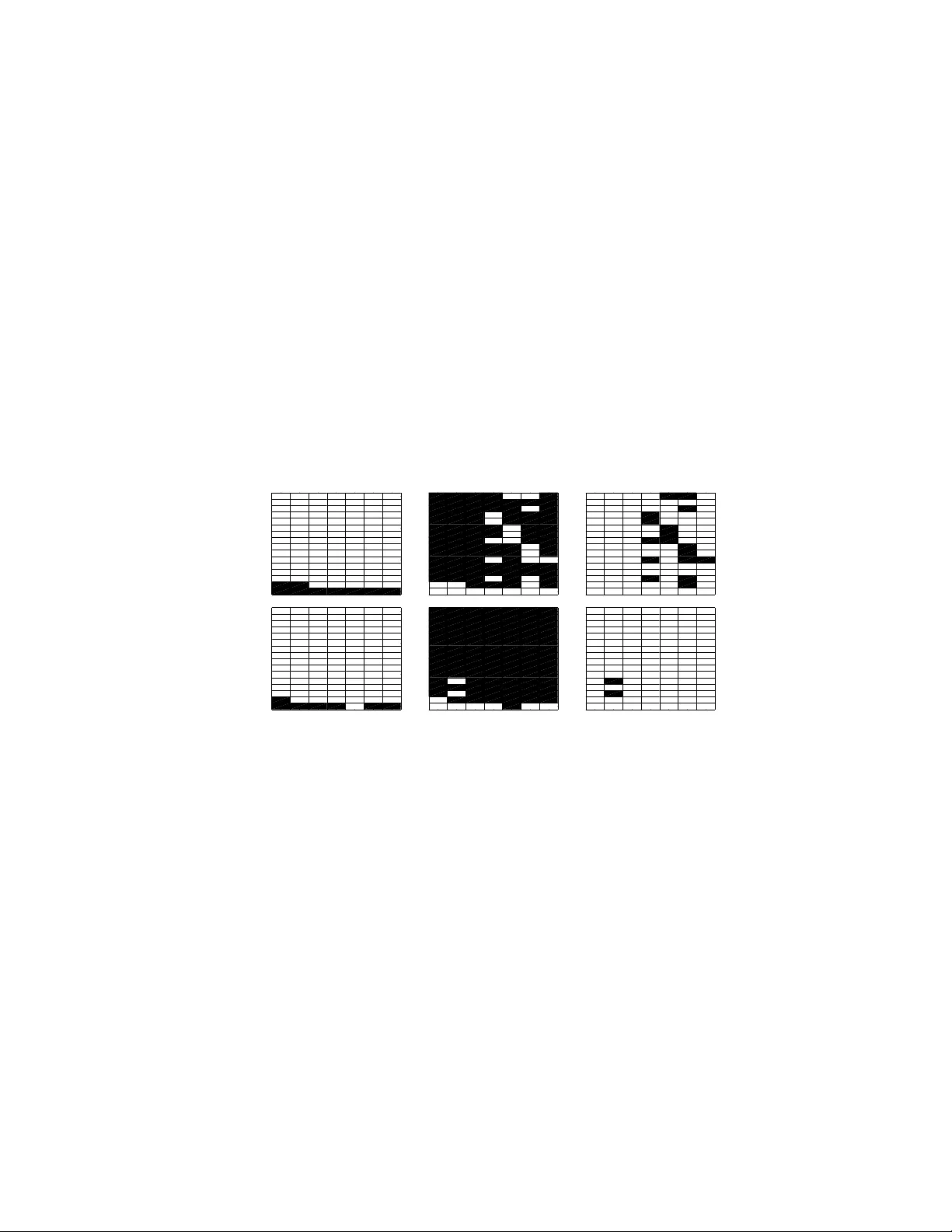
Inferenc e with Discriminati ve Posterior Jarkko Sa loj ¨ arvi † Kai Puolam ¨ aki ‡ Eerika Sa via † Samuel Kaski † Helsinki Institut e for Information T echnology Department of Information and Computer Science Helsinki Univer sity of T echnology P .O. Box 5400, FI-02015 TKK, Finland † Author belongs to the Finnish Centre of Excellence in Adaptive I nformatics Research. ‡ Author belongs to the Finnish Centre of Excellence in Algorithmi c Data Analysis Research. Abstract W e study Bay esian discriminati ve infe rence gi ven a model family p ( c, x , θ ) that is assumed to contain all our prior information b ut still kno wn to be incorrect. This falls in between “standard” Bayesian generati ve modeling and Bayesian r e- gression, where the margin p ( x , θ ) is kno wn to be u ninformativ e abo ut p ( c | x , θ ) . W e giv e an axiomatic proof that discriminative posterior is consistent for condi- tional inference; using the discriminativ e posterior is standard practice in classical Bayesian r egression , b ut we show t hat it is theoretically justified for mode l families of joint densities as well. A practical benefit compare d to Bayesian regression is that the standard me thods of hand ling missing va lues in generati ve mo deling can be extend ed into discriminati ve inference, which is useful if the amount of data is small. Compared to standard generati ve mo deling, discriminati ve posterior re- sults in better conditional inference i f the model family i s incorrect. If the model family co ntains also the true mod el, the discriminati ve posterior gi ves th e same re- sult as standard Bayesian g enerativ e modeling. Practical compu tation is done with Marko v chain Monte Carlo. 1 Introd uction Our aim is Bayesian discrimin ativ e infer ence in the case wh ere the m odel family p ( c, x , θ ) is known to be inco rrect. Here x is a d ata vector an d c its class, an d the θ are par ameters of the model family . By d iscriminative we mean pred icting the con- ditional distribution p ( c | x ) . The Bayesian ap proach of using the posterior of the gener ativ e m odel family p ( c, x , θ ) h as not been shown to be justified in this case, an d it is known that it does not always gen eralize well to n ew d ata (in case of p oint estimates, see for example 1 [1, 2, 3]; in this paper we provide a toy example that illustrates the fact for posterio r distributions). Therefo re alternative appr oaches such as Bayesian regression ar e ap- plied [4]. I t can b e argued tha t the best solu tion is to im prove the m odel family by incorpo rating more prior knowledge. Th is is not a lways possible or feasible, howe ver , and simplified mo dels are be ing generally used , often with g ood results. For example , it is often practical to use mixture models even if it is known a priori that the data can- not be faithf ully describ ed by them (see for example [5]). Th ere are go od reasons for still ap plying Bayesian- style techniqu es [6] but the gene ral problem of how to best d o inference with incorrect model families is still open. In practice, th e usual method for discrimina ti ve tasks is Bay esian regression. It dis- regards all assumptions ab out the distribution of x , and considers x only as covariates of th e mod el for c . Bayesian regression may g iv e superior results in discrimin ativ e inference , but the om ission of a generative model for x (althoug h it may be r eadily av ailable) makes it difficult to handle missing values in the data. Nu merous h euristic methods for imputing missing values have been suggested, see for example [7], b ut no theoretical argu ments of their o ptimality h av e b een presented. Here we assume that we are given a g enerative m odel family of the full data ( x , c ), and therefor e have a generative me chanism readily a vailable for imputing missing v alues. From the generative modeling per spectiv e, Bayesian regression ign ores any inf or- mation ab out c supplied by the m arginal distribution of x . This is justified if (i) th e covariates are e xplicitly chosen when designing the e xperim ental setting and hence are not no isy , or (ii) there is a sep arate set o f param eters for gen erating x on the o ne han d and c given x on the o ther, and the sets ar e assumed to be in depend ent in their p rior distribution. In the latter case the posterio r factors ou t into two parts, and the parame- ters used for gene rating x are neith er needed nor useful in the regression task. See for instance [4, 8 ] for more d etails. Howe ver , there has been no the oretical justification fo r Bayesian regression in the more general setting where th e independ ence do es not hold. For point estimates of generati ve mo dels it is well kno wn that maximizing th e joint likelihood and the co ndition al likelihoo d g iv e in gener al different results. Maximum condition al likelihoo d giv es asymp totically a better estimate of the condition al like- lihood [2] , and it can be optimized with expectation-m aximization- type pr ocedur es [9, 10]. In this paper we extend that line of work to show th at the two different approa ches, joint and con ditional mod eling, result in different posterior distributions which are asymp totically equ al o nly if th e true model is w ithin th e mode l family . W e giv e an axiomatic justification to the discriminati ve posterior, a nd demonstrate empiri- cally th at it works as e xpected . If there are no covariates, the discriminati ve posterior is the same as the standard posterior of joint density modeling, that is, ordinar y Bayesian inference . T o o ur kn owledge the extension from point estimates to a p osterior distribution is new . W e ar e aware of only o ne sug gestion, the so-called supervised po sterior [11], which also has empirical supp ort in the sense of m aximum a p osteriori estimates [12]. The posterior has, howe ver , on ly been justified heuristically . For the pur pose of r egression, the discrimin ativ e po sterior makes it possible to use more gen eral model stru ctures than stand ard Bayesian regression ; in essence any generative model family can be used . In add ition to giving a g eneral justification 2 to Bay esian r egression-type modelin g, pre dictions given a ge nerative model family p ( c, x , θ ) should b e better if the whole model is ( at least ap proxim ately) correct. The additional ben efit is that th e use of the full g enerative model gi ves a principled way o f handling missing values. The gain ed a dvantage, co mpared to using the standard no n- discriminative posterior, is that the prediction s shou ld b e m ore accu rate assuming the model family is incorrect. In this p aper, we present the necessary back groun d and definitio ns in Section 2. The discriminative posterior is derived briefly from a set of fi ve axioms in Section 3; the full proof is included as an append ix. There is a close resemblance to Cox axioms, and stand ard Bayesian inference can inde ed be d erived also from this set. However , the ne w axioms all ow also inference in the case where the m odel manifold is known to be inadequa te. In section 4 we sh ow that discriminative p osterior can be extended in a standard mann er [7] to handle data missing at random. In Section 5 we pre sent some experimental e vidence that the discriminative posterio r beha ves as e xpected . 2 Aims and Definitions In this paper, we prove the following two claims; the claims follow from Theorem 3.1, discriminative po sterior, wh ich is the main result of this paper . W ell-known Giv en a d iscriminative mod el, a model p ( c | x ; θ ) f or the condition al density , Bayesian regression results i n consistent cond itional inference. New Gi ven a joint density model p ( c, x | θ ) , discr iminative posterior results in co n- sistent condition al inference. In accordan ce with [13], we call in ference consistent if the utility is maximized with large data sets. This p aper pr oves bo th of the above claims. Notice that although th e claim 1 is well known, it has not been proven, aside f rom the special case where the priors for the m argin x and c | x are independ ent, as discussed in th e introd uction and in [4]. 2.1 Setup Throu ghout the paper , observations are denoted by ( c, x ) , an d assumed to b e i.i.d. W e use Θ to denote the set of all possible m odels that could generate the observations. Models that a re applicable in practice are restricted to a lower dimen sional manifold Θ of models, Θ ⊆ Θ . In other words, the subspac e Θ defin es ou r mo del fa mily , in this work denoted by a distrib ution p ( c, x , θ ) parame terized by θ ∈ Θ . There exists a mode l in Θ which describes the “ true” model, wh ich h as actu ally generated the ob servations and is typically u nknown. W ith sligh t abuse o f no tation we den ote this mo del by ˜ θ ∈ Θ , with the un derstandin g that it may be outside o ur parametric mo del family . I n fact, in pr actice no probab ilistic model is perfectly tru e and is false to some extent, that is, the da ta has usually no t been gene rated by a mod el in our model family , ˜ θ / ∈ Θ . 3 The distribution induc ed in the model p arameter space Θ after ob serving the data D = { ( c, x ) } n i =1 is referred to as a po sterior . By standard posterio r we m ean the posterior obta ined fro m Bayes formula using a fu ll join t density model. In this pap er we discuss the discriminative p osterior, which is o btained from axioms 1–5 belo w . 2.2 Utility Function and P oint Estimates In this subsection, we in troduce the research pro blem by recapitulating the known dif- ference between p oint estimates o f joint and cond itional likelihoo d. W e present th e point estimates in term s of Kullback-Leibler divergences, in a fo rm that allows ge ner- alizing from point estimates to the posterior distribution in section 3. Bayesian infer ence can be derived in a decision theoretic framework as maximiza- tion of the expected u tility of the decision maker [ 14]. In genera l, the cho ice of the utility f unction is subjective. Howe ver , several arguments for using log -prob ability as utility function can be made, see for example [14]. When i nspecting a full ge nerative mo del at th e limit where the amount o f d ata is in- finite, the joint posterior distribution p j ( θ | D ) ∝ p ( θ ) Q ( c, x ) ∈ D p ( c, x | θ ) becomes a point solution , p j ( θ | D ) = δ ( θ − ˆ θ ) . 1 An accur ate approx imation of the log-likelihoo d is pro duced by a utility function m inimizing the approxima tion er ror K J OI N T between the point estimate ˆ θ J OI N T and the true model ˜ θ as follows: ˆ θ J OI N T = arg min θ ∈ Θ K J OI N T ( ˜ θ , θ ) wher e K J OI N T ( ˜ θ , θ ) = X c Z p ( c, x | ˜ θ ) log p ( c, x | ˜ θ ) p ( c, x | θ ) d x , (1) If the tru e mod el is in the mo del family , that is, ˜ θ ∈ Θ , equ ation (1) can b e minimized to zero a nd the r esulting po int estimate is effecti vely the MAP solu tion. If ˜ θ / ∈ Θ th e resulting point estimate is the best estimate of the tru e joint d istribution p ( c, x | ˜ θ ) with respect to K J OI N T . Howe ver , th e joint estimate may not be optimal if we are interested in approx imat- ing some other q uantity than the likeliho od. Consider the problem o f finding the best point estimate ˆ θ C ON D for the con ditional distribution p ( c | x , θ ) . The average KL- div ergence between the true co nditional d istribution at ˜ θ and its estimate a t θ is given by K C ON D ( ˜ θ, θ ) = Z p ( x | ˜ θ ) X c p ( c | x , ˜ θ ) lo g p ( c | x , ˜ θ ) p ( c | x , θ ) d x , (2) and the best point estimate with respect to K C ON D is ˆ θ C ON D = arg min θ ∈ Θ K C ON D ( ˜ θ , θ ) . (3) By equations (1) and (2) we may write K J OI N T ( ˜ θ, θ ) = K C ON D ( ˜ θ, θ ) + Z p ( x | ˜ θ ) log p ( x | ˜ θ ) p ( x | θ ) d x . (4) 1 Strictl y spea king, the posterior can also have multiple modes; we will not treat these special cases here but th ey do not restric t the generali ty . 4 Therefo re the point estimates ˆ θ J OI N T and ˆ θ C ON D are different in gen eral. If the mod el that has ge nerated the d ata does n ot belon g to the m odel family , that is ˜ θ / ∈ Θ , then by Equation (4) the joint estimate is generally worse than th e conditional estimate in condition al inference, measured in terms of condition al likelihood. See also [2]. 2.3 Discriminative versus gener ative models A discriminative mo del does not make any ass ump tions on t he distribution of the mar - gin of x . Th at is, it do es not incorpo rate a generative model for x , and can b e interpreted to rather use the empirical distribution of p ( x ) as its margin [ 15]. A gen erative model, o n the other hand, assumes a specific param etric form for the full d istribution p ( c, x , θ ) . A ge nerative model can be learned either as a jo int d ensity model or in a discriminativ e manner . Our point in this paper is that the selection corre- sponds to cho osing the utility fun ction; this is actually o ur fifth axio m in section 3 . In joint d ensity mo deling the utility is to m odel the full distribution p ( c, x ) as ac curately as possible, which c orrespon ds to co mputing the stand ard po sterior inco rporatin g th e likelihood functio n. In d iscriminative learn ing the utility is to mod el the co nditional distribution of p ( c | x ) , and the result is a d iscriminative poster ior in corpo rating the condition al likelihoo d. A generative model op timized in discriminative manne r is re- ferred to as a discriminative join t density model in the following. For generative mo dels and i n case o f point estimates, if the model f amily is co rrect, a m aximum likelihood (ML) solutio n is better for pred icting p ( c | x ) than maximu m condition al likelihoo d (CML). They ha ve the same maximum, but the asymptotic vari- ance of CML estimate is higher [16]. Howe ver , in case of in correct models, a maximum condition al likelihood est imate is better than maximum lik elihood [2]. For an example illustrating that CML can be better than ML in predicting p ( c | x ) , see [17]. Since the discr iminative joint d ensity m odel has a mo re r estricted mod el stru cture than Bayesian regression, we expect it to perf orm better with small amoun ts o f data. More formally , later in Theorem 3.1 we move from point estimate of Equation (3) to a discriminative posterio r distribution p d ( θ | D ) over the m odel parame ters θ in Θ . Sin ce the posterio r is nor malized to unity , R Θ p d ( θ | D ) dθ = 1 , th e values of the p osterior p d ( θ | D ) are generally smaller for larger model families; the posterior is more dif fuse. Equation (2) can be generalized to the expectation of the approximation error , E p d ( θ | D ) h K C ON D ( ˜ θ, θ ) i = − Z X c p ( x , c | ˜ θ ) p d ( θ | D ) log p ( c | x , θ ) d x dθ +const . (5) The expected appro ximation error is sm all when b oth the d iscriminative posterior dis- tribution p d ( θ | D ) and th e conditio nal likeliho od p ( c | x , θ ) are large at the same time. For small amounts of data, if the model family is too large, t he values of the pos- terior p d ( θ | D ) ar e small. The d iscriminative join t density model h as a mor e re stricted model family than that of the Bayesian regression, an d hence the values of the po ste- rior are larger . If the model is ap proxim ately co rrect, the discrimin ativ e joint density model will have a smaller appr oximation error than the Bayesian regression, that is, p ( c | x , θ ) is large somewhere in Θ . This is ana logous to selecting the model family that m aximizes the evidence (in our case the expected co nditional log-likelihood ) in 5 Bayesian infer ence; choo sing a m odel family th at is too co mplex leads to small evi- dence (see, e.g., [18]). T he d ifference to the traditio nal Bay esian in ference is th at we do not requir e that the true data gene rating distribution ˜ θ is con tained in the param eter space Θ u nder consideratio n. 3 Axiomatic Derivation of Discriminative P osterior In this section we generalize the poin t estimate ˆ θ C ON D presented in sectio n 2.2 to a discriminative posterior distribution over θ ∈ Θ . Theorem 3.1 (Discrimi native posterior distrib ution) It follows fr om a xioms 1–6 listed below tha t, g iven d ata D = { ( c i , x i ) } n i =1 , the discriminative posterior distribution p d ( θ | D ) is of the form p d ( θ | D ) ∝ p ( θ ) Y ( c, x ) ∈ D p ( c | x , θ ) . The pr edictive distrib ution for n ew ˜ x , ob tained by inte grating over this posterior , p ( c | ˜ x , D ) = R p d ( θ | D ) p ( c | ˜ x , θ ) dθ , is consistent for co nditiona l infer ence. Th at is, p d is consistent for the utility of conditiona l likelihood. The discriminative posterior follo ws from requiring the following axioms to hold: 1. T he posterio r p d ( θ | D ) c an be r epresented by non -negative real numbers that satisfy R Θ p d ( θ | D ) dθ = 1 . 2. A mo del θ ∈ Θ ca n be r epresented as a fu nction h (( c, x ) , θ ) that m aps the observations ( c, x ) to r eal numbers. 3. T he p osterior, after observin g a data set D followed by an obser vation ( c, x ) , is giv en by p d ( θ | D ∪ ( c, x )) = F ( h (( c, x ) , θ ) , p d ( θ | D )) , where F is a twice differentiable function in both of its param eters. 4. E xchang eability: The v alue of the posterior is independent of the or dering of the observations. That is, the posterior after two observations ( c, x ) and ( c ′ , x ′ ) is the same irrespective of their ordering: F ( h (( c ′ , x ′ ) , θ ) , p d ( θ | ( c, x ) ∪ D )) = F ( h (( c, x ) , θ ) , p d ( θ | ( c ′ , x ′ ) ∪ D )) . 5. T he p osterior must agree with the utility . For ˜ θ ∈ Θ , and θ 1 , θ 2 ∈ Θ , the following condition i s satisfied: p d ( θ 1 | D ˜ θ ) ≤ p d ( θ 2 | D ˜ θ ) ⇔ K C ON D ( ˜ θ , θ 1 ) ≥ K C ON D ( ˜ θ, θ 2 ) , where D ˜ θ is a very la rge data set sampled from p ( c, x | ˜ θ ) . W e fur ther assume that th e d iscriminative posterior s p d at θ 1 and θ 2 are e qual on ly if the corr espond- ing condition al KL-diver gences K C ON D are equal. 6 The first axiom above is simply a req uiremen t that the posterio r is a p robab ility distri- bution in the param eter space. The second axiom d efines a model in gen eral te rms; we define it as a ma pping from ev ent space into a real number . The third axiom makes smoothness assumptions on the posterio r . Th e reason for the ax iom is techn ical; the smoothness is used in the pro ofs. Cox [19] m akes similar assumptions, and our proof therefore holds in the same scope as Cox’ s; see [20]. The fourth axiom requir es exch angeability ; the sh ape of the posterior distribution should not dep end on the order in which the observations are made. This deviates slightly fro m analo gous earlier pro ofs fo r standar d Bayesian in ference, which ha ve rather used the requir ement of associativity [1 9] or included it a s an addition al con- straint in modeling after presenting the axioms [14]. The fifth axiom states, in essence, th at asym ptotically (at the limit of a large but finite data set) the shap e o f the posterior is such th at the poster ior is always smaller if the “d istance” K C ON D ( ˜ θ, θ ) is larger . If the oppo site would b e tru e, th e integral over the d iscriminative p osterior would give larger weight to solutions further away from the true model, leading to a larger error measured by K C ON D ( ˜ θ , θ ) . Axioms 1–5 ar e sufficient to fix th e discriminative poster ior , up to a monoto nic transform ation. T o fix the mono tonic transformation we introduce the sixth axiom: 6. For fixed x the model re duces to the stand ard po sterior . For th e data set D x = { ( c, x ′ ) ∈ D | x ′ = x } , the discrimin ativ e posterior p d ( θ | D x ) match es the standard posterior p x ( c | θ ) ≡ p ( c | x , θ ) . W e use p ( θ ) = p d ( θ | ∅ ) to denote the p osterior when no data is observed ( prior distribution ). Proof The proof is in the Appendix. For clarity of presenta tion, we additionally sketch the proof in the following. Proposition 3.2 ( F is isomorphic to multiplication) It fo llows fr om axiom 4 tha t the function F is of the form f ( F ( h (( c, x ) , θ ) , p d ( θ | D )) ∝ h (( c, x ) , θ ) f ( p d ( θ | D )) , (6) where f is a monoton ic function which we, by co nv ention, fix to the identity function. 2 The pro blem then red uces to find ing a f unction al fo rm for h (( c, x ) , θ ) . Utilizing both the equality part and the inequality part of axiom 5, the follo wing propo sition can be derived. Proposition 3.3 It follows fr om axiom 5 that h (( c, x ) , θ ) ∝ p ( c | x , θ ) A where A > 0 . (7) Finally , the axiom 6 effecti vely states that we decide to follow the Bayesian c onv ention for a fixed x , that is, to set A = 1 . 2 W e follo w here Cox [19] and subsequent wor k, see e.g. [20]. A differe nce which does not af fect the need for the con vent ion is that usuall y multipl icati vit y is de riv ed based on t he assumptio n of associati vit y , not ex changeab ility . Our setup is sli ghtly differ ent from Cox, since instead of upd ating beliefs on e vent s, we here consider updat ing beliefs in a family of models. 7 4 Modeling Missing Data New Discriminativ e p osterior giv es a theoretically justified way of handlin g m issing values in discriminative tasks. Discriminative mo dels cann ot readily handle co mpon ents missing f rom the data vector, since the d ata is used only as covariates. Howev er, standard methods of h andling miss- ing data with generative mo dels [7] can be applied with the discriminative po sterior . The additiona l assumption we need to make is a model for which data are miss ing. Below we derive th e formulas fo r the comm on case of d ata m issing independ ently at random . Exten sions inc orpor ating pr ior info rmation of the process by which th e d ata are missing are straightforward, although possibly not tri vial. Write the obser vations x = ( x 1 , x 2 ) . Assume that x 1 can be missing and denote a missing observation by x 1 = ⊘ . The task is still to predic t c by p ( c | x 1 , x 2 ) . Since we are g iv en a m odel fo r the joint d istribution wh ich is assumed to be ap- proxim ately co rrect, it will be used to model the missing data. W e deno te this by q ( c, x 1 , x 2 | θ ′ ) , x 1 6 = ⊘ , with a p rior q ( θ ′ ) , θ ′ ∈ Θ ′ . W e furthe r d enote the parame- ters of the missing data mechan ism by λ . Now , similar to joint density m odeling , if the priors fo r th e join t model, q ( θ ′ ) , and missing -data mec hanism, g ( λ ) , are indepen dent, the missing data mechanism is ig norab le [7]. I n other words, the posterior that takes the missing data into account can be written as p d ( θ | D ) ∝ q ( θ ′ ) g ( λ ) Y y ∈ D f ull q ( c | x 1 , x 2 , θ ′ ) Y y ∈ D missing q ( c | x 2 , θ ′ ) , (8) where y = ( c, x 1 , x 2 ) and we have used to D f ull and D missing to denote the portion s of data set with x 1 6 = ⊘ and x 1 = ⊘ , respectively . Equation (8) has b een obtained by using q to con struct a mod el family in which the data is missing indepe ndently at rand om with probab ility λ , having a prior g ( λ ) . That is, we define a m odel family that g enerates the missing d ata in ad dition to th e non-m issing data, p ( c, x 1 , x 2 | θ ) ≡  (1 − λ ) q ( c, x 1 , x 2 | θ ′ ) , x 1 6 = ⊘ λ R supp( x 1 ) \⊘ q ( c, x , x 2 | θ ′ ) d x = λq ( c, x 2 | θ ′ ) , x 1 = ⊘ , (9) where θ ∈ Θ and supp( x 1 ) denotes the supp ort o f x 1 . The parame ter space Θ is spanned by θ ′ ∈ Θ ′ and λ . The equatio n (8) follows directly by applying Theorem 3.1 to p ( c | x 1 , x 2 , θ ) . 3 Notice th at th e po sterior for θ ′ of (8) is indep endent of λ . Th e division to x 1 and x 2 can be made separately f or each data item. The items can have different numb ers of missing comp onents, each co mpon ent k having a pr obability λ k of being missing. 3 Notice that p ( c | x 1 , x 2 , θ ) = q ( c | x 1 , x 2 , θ ′ ) when x 1 6 = ⊘ , and p ( c | x 1 = ⊘ , x 2 , θ ) = q ( c | x 2 , θ ′ ) . 8 5 Experiments 5.1 Implementation of Discriminative S ampling The discrimin ativ e posterior can be sam pled with a n ord inary Metrop olis-Hastings al- gorithm where the standard p osterior p ( θ | D ) ∝ Q n i =1 p ( c i , x i | θ ) p ( θ ) is simp ly replaced b y the d iscriminative version p d ( θ | D ) ∝ Q n i =1 p ( c i | x i , θ ) p ( θ ) , where p ( c i | x i , θ ) = p ( c i ,x i | θ ) p ( x i | θ ) . In MCMC sam pling o f the discriminative posterior, the n ormalizatio n ter m of the condition al likelihood p oses prob lems, since it in volv es a marginalization over the class variable c and latent variables z , that is, p ( x i | θ ) = P c R supp( z ) p ( x i , z , c | θ ) dz . In case o f discrete latent variables, such as in m ixture models, the marginalization re- duces to simple summations and can be computed exactly and ef ficiently . If the mode l contains continuou s latent variables the integral needs to be e valuated n umerically . 5.2 Pe rformanc e as a function of the incorrectn ess o f the model W e first s et up a toy exam ple wh ere the distance between the mo del family and the true model is varied. 5.2.1 Background In this experim ent we com pare th e pe rforma nce o f logistic regression an d a mixtu re model. L ogistic regression w as chosen sinc e many of the discriminative models can be seen as extensions of it, f or example con ditional r andom fields [8]. In case of lo gistic regression, the follo wing theorem exists: Theorem 5.1 [21] F or a k-cla ss cla ssification pr oblem with equa l priors, th e pairwise log-od ds ratio of the class p osteriors is affine if and o nly if th e cla ss cond itional distrib utions b elong to any fixed exponential family . That is, the mo del family of logistic regression incorpor ates the model family of any generative exponential (mixture) model 4 . A direct in terpretation is that a ny generative exponential family mixtu re model defines a sma ller subspace within the p arametric space of the logistic regression model. Since the mod el family o f logistic regression is larger, it is asymp totically better, but if the number of data is small, generative mo dels can be better due to the restricted parameter space; see fo r examp le [3] f or a co mparison of na iv e Bayes and log istic re- gression. This happens if the particular model family is at least approximately correct. 5.2.2 Experiment The tru e model gen erates ten- dimensiona l data x fro m the two-comp onent mixture p ( x ) = P 2 j =1 1 2 × p ( x | ˜ µ j , ˜ σ j ) , w here j indexes the mixture com ponen t, and p ( x | 4 Banerje e [21] provides a proof also for conditi onal random fields. 9 ˜ µ j , ˜ σ j ) is a Gaussian with mean ˜ µ j and stan dard d eviation ˜ σ j . The data is lab eled accordin g to the generating mixtu re co mpon ent (i.e., the “class” variable) j ∈ { 1 , 2 } . T wo of t he ten dimensions contain information about the class. The “true” parameters, used to generate the data, on these dimensions are ˜ µ 1 = 5 , ˜ σ 1 = 2 , and ˜ µ 2 = 9 , ˜ σ 2 = 2 . T he remain ing eight d imensions ar e Gaussian noise with ˜ µ = 9 , ˜ σ = 2 for bo th compon ents. The “inco rrect” generativ e model used for inference is a mix ture of two Gaussians where the v ariances are constrained to be σ j = k · µ j + 2 . W ith increasing k th e model family thus draws fu rther away from the tru e mo del. W e assum e fo r both of th e µ j a Gaussian prior p ( µ j | m, s ) ha ving the same fixed hyperparam eters 5 m = 7 , s = 7 for all dimension s. Data sets were gener ated from the tr ue mode l with 10000 test data points and a varying number of training d ata points ( N D = { 32 , 64 , 128 , 256 , 512 , 1024 } ). Both the d iscriminative and standard posteriors we re sampled for the model. Th e g oodne ss of the mod els was evaluated by perplexity of conditional likeliho od on th e test d ata set. Standard and discriminative posteriors of the incorrect gener ativ e mod el are com- pared against Bayesian logistic regression . A uniform prior for the pa rameters β of the logistic regression mod el was assumed. As m entioned in subsection 5.2.1 ab ove, the Gaussian naiv e Bay es and logistic regression are connected ( see fo r example [22] for e xact mapping between the parameters). The parameter spa ce of the logistic model incorpo rates the true mode l as well as th e inco rrect mo del family , an d is the refore the optimal discr iminative model fo r this toy data. Howe ver , since the param eter space o f the lo gistic r egression mod el is lar ger, th e m odel is e xpected to need more data samples for good predictions. The m odels p erform as exp ected (Figur e 1). The m odel family of ou r incorr ect model was chosen such that it contains useful prior k nowledge abou t the distribution of x . Compared with logistic regression , the model family b ecomes mo re restricted which is beneficial for sma ll learn ing d ata sets (see Figu re 1a). Comp ared to joint density sampling, discriminative sampling results in better pr edictions o f the class c when the model family is incorrect. The mo dels were compared mor e quantitatively by repeating the samplin g ten times for a fixed value of k = 2 for each of the learn ing data set sizes; in every repeat also a new data set was gen erated. The resu lts in Figu re 2 co nfirm the qu alitativ e findings of Figure 1. The p osterior was sampled w ith Metro polis-Hastings algo rithm with a Gaussian jump kernel. In case of joint d ensity and discr iminative samp ling, thr ee chain s were sampled with a burn-in of 50 0 iteration s each, afte r wh ich every fifth samp le was col- lected. Bayesian regression req uired m ore samples f or conv ergence, so a burn- in of 5500 samples was used. Conver gence was estimated when carr ying out experim ents for Figu re 2 ; the length o f sam pling ch ains was set suc h th at the con fidence intervals for each o f the models was roug hly th e same. Th e total number o f s amples w as 900 per chain. The wid th o f jump kerne l was chosen as a linear fu nction of data such that th e acceptance rate was b etween 0.2– 0.4 [4] as the amou nt of data was increased. Selectio n was carried out by preliminary tests with dif ferent random seeds. 5 The model is thus slightly incorrec t ev en with k = 0 . 10 Missing Dat a. The experimen t with toy data is co ntinued in a setting where 5 0% o f the learning data are missing at random . MCMC sampling was carried out as d escribed above. F or th e logistic regression model, a multiple imputatio n scheme is app lied, as rec ommend ed in [ 4]. In or der to have samp ling conditions comparab le to sampling from a generativ e model, each sam- pling ch ain used o ne impu ted data set. Imputation was car ried ou t with th e gen erative model (rep resenting our curre nt best knowledge, d iffering fro m the true joint mod el, howe ver). As can b e seen from Figure 1 , discrimina tiv e samp ling is better than joint d ensity sampling when the model is incorr ect. T he perform ance of Bayesian regression seems to be affected heavily by the incorrect generative mo del used to generate missing data. As can be seen fr om Figure 2, sur prisingly the Bayesian r egression is e ven worse than standard p osterior . The perfo rmance cou ld be in creased by imputing more than one data sets with the cost of additional computatio nal complexity , howev er . Joint density MCMC Discriminative MCMC Bayesian regression a) 32 64 128 256 512 1024 2048 0 1 2 3 32 64 128 256 512 1024 2048 0 1 2 3 32 64 128 256 512 1024 2048 0 1 2 3 b) 32 64 128 256 512 1024 2048 0 1 2 3 32 64 128 256 512 1024 2048 0 1 2 3 32 64 128 256 512 1024 2048 0 1 2 3 Figure 1: A comp arison of joint density sampling, d iscriminative sam pling, and Bayesian regression, a) Fu ll data, b) 50% of the data m issing. Grid poin ts wher e the method is better than othe rs are marked with black. The X-axis d enotes the amou nt of data, and Y -axis the deviance o f the the mode l family from the “tru e” model (i.e., the value of k ). The methods are prone to samp ling error, but the following general conclusion s can be made: Bayesian generative modelin g ( “Joint density MCMC”) is best when th e mode l family is ap proxim ately correct. Discrimina ti ve po sterior (“Dis- criminative MCMC”) is better wh en the m odel is inco rrect and the learning data set is small. As the amo unt of data is incr eased, Bayesian regression a nd discriminative posterior show roughly equal perform ance (see also Figure 2). 5.3 Document Modeling As a d emonstratio n in a practical d omain we ap plied the d iscriminative posterior to docume nt classification. W e used the Reuters data set [23], of which we selected a 11 a) b) 32 64 128 256 512 1024 2048 1.2 1.3 1.4 1.5 1.6 1.7 1.8 1.9 2 32 64 128 256 512 1024 2048 1.2 1.3 1.4 1.5 1.6 1.7 1.8 1.9 2 Figure 2: A co mparison of joint d ensity sampling (dotted line), discriminative sam- pling (solid lin e), and Bayesian regression (d ashed line) with an inco rrect mo del. X- axis: le arning d ata set size, Y -axis: per plexity . Also the 95 % con fidence intervals are p lotted (with the thin lines). Logistic regression pe rforms sign ificantly worse than discriminative posterior with small data set sizes, whereas with large data sets the p er- forman ce is roug hly equ al. Join t density modeling is consistently worse. Th e model was fixed to k = 2 , ten ind ividual runs were carried out in order to compu te 95 % confidenc e intervals. a) Full data, b) 50% of the data missing. subset o f 1 100 d ocumen ts f rom fo ur categor ies ( CCA T , ECA T , GCA T , MCA T). Each selected document was classified to exactly one of the four classes. As a preprocessing stage, we cho se the 25 mo st infor mative words within the trainin g set of 10 0 docu - ments, having th e highest mutu al in formation between classes and words [24]. Th e remaining 1000 documen ts were used as a test set. W e first a pplied a mixture of un igrams mo del ( MUM, see Figu re 3 left) [25]. The model assumes that each docu ment is generate d f rom a mixtur e of M h idden “top- ics, ” p ( x i | θ ) = P M j =1 π ( j ) p ( x i | β j ) , where j is the in dex of th e top ic, and β j the multinomia l parameters that generate words from the topic. The vector x i contains the observed word cou nts (with a total o f N W ) fo r d ocumen t i , an d π ( j ) is the probabil- ity of g enerating words from the topic j . The u sual appr oach [4] for mode ling paired data { x i , c i } N D i =1 by a jo int de nsity m ixture mo del was applied; c was assoc iated with the label o f the mixtur e compon ent f rom which the d ata is assum ed to b e gener ated. Dirichlet prio rs were used for th e β , π , with h yperp arameters set to 25 and 1, respec- ti vely . W e used th e simp lest for m of MUM containin g one top ic vector per class. The sampler used Metropolis-Hastings with a Gaussian jump kernel. The kernel wid th was chosen such that the acceptance rate was roughly 0.2 [4]. As an example o f a model with con tinous hidden variables, we implemen ted the Latent Dirichlet Allocation (LDA) or discrete PCA mo del [26, 27]. W e constru cted a variant of the model th at generates also th e classes, shown in Figure 3 (right) . The topolog y o f the mo del is a mixture of LD As; the generatin g mixtur e compon ent z c is fir st sampled f rom π c . T he componen t indexes a row in the matrix α , an d (for simplicity) con tains a direct m apping to c . Now , giv en α , the gen erative model for 12 words is an o rdinary L D A. Th e π is a topic d istribution drawn individually for each docume nt d from a Dir ichlet with p arameters α ( z c ) , that is, Dirichlet ( α ( z c )) . Ea ch word w nd belongs to one topic z nd which is picked from Multinomial ( π ) . Th e w ord is then generated from Multinomial ( β ( z nd , · )) , where z nd indexes a row in the matrix β . W e assume a Dirichlet prior fo r th e β , with hyperparameters set to 2 , Dirichlet prior for the α , with hyperp arameters set to 1, and a Dirichlet prior for π c with hyperparam eters equal to 5 0. The param eter values were set in initial test run s (with a separate d ata set from the Reuters corp us). Four topic vectors were assumed, making the mo del structure similar to [2 8]. The difference to MUM is that in LDA-type mod els a document can be generated from se veral topics. Sampling was carried out using Metropolis-Hastings with a Gaussian jump kernel, where the kernel wid th was chosen su ch that the acceptance rate was ro ughly 0.2 [4]. The necessary integrals w ere com puted with Monte Carlo integration. Th e conver gence of integration was monitored with a jackknife estima te of stand ard error [ 29]; sampling was ended when the estimate was less than 5 % of the v alue of the integral. The length of burn-in was 1 00 iterations, after which every tenth sample was p icked. The total number of collected samp les was 100. The p robab ilities were clipp ed to the rang e [ e − 22 , 1] . π z w β N W c N D π z w β N W c N D z c α π c Figure 3: Left: Mix ture of Unigra ms. Right: M ixture of Latent Dirichlet Allocatio n models. 5.3.1 Results Discriminative sam pling is better for both models (T ab le 1). T able 1: Com parison of samplin g from the or dinary posterior (jMCMC) an d discrimi- native posterior (d MCMC) for two mode l families: M ixture of Unigra ms (MUM) and mixture of Latent Dirichlet Allocation models (mLD A). The figures are perplexities of the 100 0 docume nt test set; th ere were 100 learnin g data poin ts. Small per plexity is better; random guessing gi ves perplexity of 4. Model dMCMC jMCMC Conditional ML MUM 2.56 3.98 4.84 mLD A 2.36 3.92 3.14 13 6 Discussion W e h av e introdu ced a principled w ay of makin g conditional inference with a discrimi- native po sterior . Compare d to standard joint posterior density , discriminative posterior results in better inferen ce when th e mo del family is in correct, which is usually the case. Compared to p urely discriminative modeling, discriminativ e posterior is better in case of small data sets if the model family is at least approxim ately co rrect. Addition ally , we have introd uced a ju stified method for incorp orating missing data into discriminative modeling . Joint density modeling, discrim inative joint den sity modeling , and Bayesian regres- sion can b e seen as mak ing different assumptions on th e margin model p ( x | θ ) . Joint density modeling assumes the model family to be correct, and hence als o the mod el of x margin to be correc t. If this assum ption holds, the discrimin ativ e posterior and joint density modeling will asym ptotically giv e th e same resu lt. On the other hand, if th e as- sumption does not hold, the d iscriminative joint den sity mo deling will asy mptotically giv e better or at least as good resu lts. Discriminative joint density modeling assumes that the margin model p ( x | θ ) may be incorrect, b ut the conditional model p ( c | x , θ ) , derived fr om the joint model that includes the mode l for the margin, is in itself at least approx imately correct. Then inf erence is best made with discriminative posterior as in this paper . Finally , if the m odel family is completely in correct — or if there is lots of data — a larger , discriminati ve model family and Bayesian regression sh ould be used. Another approach to the same problem was sug gested in [30 ], where the traditional generative view to d iscriminative modeling h as b een extend ed b y comp lementing the condition al model for p ( c | x , θ ) with a m odel for p ( x | θ ′ ) , to form th e joint de nsity model p ( c, x | θ, θ ′ ) = p ( c | x , θ ) p ( x | θ ′ ) . That is, a larger mod el family is postulated with addition al par ameters θ ′ for mod eling th e marginal x . The c ondition al density model p ( c | x , θ ) is derived by Bayes r ule from a formula for the joint density , p ( c, x | θ ) , and the model for the marginal p ( x | θ ′ ) is obtained by marginalizing it. This co nceptualizatio n is very useful for semisuperv ised learning; the dep enden cy between θ and θ ′ can be tu ned by choosing a su itable p rior, which allows balan cing between discrimin ativ e and genera ti ve modeling. The o ptimum for sem isupervised learning is foun d in between th e two extremes. The appro ach of [30] c ontains our discriminative posterior distribution as a special case in th e limit where the priors a re indepen dent, that is, p ( θ, θ ′ ) = p ( θ ) p ( θ ′ ) where the parameters θ and θ ′ can be treated indepen dently . Also [30] can be viewed as g iving a th eoretical justification for Bayesian discrim - inativ e le arning, based on gene rativ e mod eling. The work introduce s a meth od of ex- tending a fully discriminative model into a gener ativ e model, making discriminative learning a spec ial case of optimizing the likelihood ( that is, the case where priors sepa- rate). Our work st arts from different assumptions. W e assume that the utility functions can b e different, dep ending on the g oal o f th e modeler . As we show in this pap er , the requirem ent of our axiom 5 that the utility should agree with the posterior will e ventu- ally lead us to the proper form of the posterior . Here we chose conditional in ference as the utility , obtain ing a discriminativ e posterior . If the utility had b een joint mod eling o f ( c, x ) , we would ha ve obtained t he standard p osterior (the case of no cov ariates). I f the giv en model is incorrect the different utilities lead to dif ferent learning schemes. From 14 this point o f view , the approach of [3 0] is pr incipled o nly if th e “true” mod el belong s to the postulated larger model family p ( c, x | θ , θ ′ ) . As a practical matter , ef ficient implementation of samp ling from the discriminati ve posterior will require more work. The sampling schemes applied in this paper are sim- ple and compu tationally in tensiv e; there exist se veral more advanced m ethods which should be tested. Acknowledgmen ts This w ork was supported in part by the P ASCAL2 Network of Excellence of the Euro- pean Community . T his publication only reflects the authors’ views. Refer ences [1] B. Efron . The efficiency of log istic regression com pared to normal discrimina nt analysis. Journal of the American Statistical Association , 70:892– 898, 1975. [2] Arthur N ´ adas, David Nahamoo, and M ichael A. Pich eny . On a mod el-robust training method for speech recognition. IEEE transactions on Acoustics, Speech, and Signal Pr ocessing , 39(9):14 32–14 36, 1988. [3] Andrew Y . Ng and Michael I. Jo rdan. On discriminative vs. gene rativ e classi- fiers: A comparison of lo gistic regression and naive Bayes. In T . G. Dietter ich, S. Becker , an d Z. Ghahramani, editors, Advances in N eural Information Pr ocess- ing Systems 14 , pages 841–84 8. MIT Press, Cambridge, MA, 2002. [4] Andrew Gelm an, John B. Carlin, Hal S. Stern, and Donald B. Rubin. B ayesian Data Analysis (2nd edition) . Chapm an & Hall/CRC, Boca Raton, FL, 2003. [5] Geoffrey J. McLachlan and David Peel. F inite Mixtur e Models . John W iley & Sons, New Y ork, NY , 2000 . [6] L. K. Hansen . Bayesian averaging is well-temper ated. In Sara A. So lla, T odd K. Leen, an d Klaus-Robert M ¨ uller , edito rs, A dvances in Neural Info rmation Pr o- cessing Systems 12 , pages 265–2 71. MIT Press, 2000. [7] Roderick J.A. Litte an d Don ald B. Rub in. Statistical an alysis with missing data . John W ile y & Sons, Inc. , Hoboken, NJ, 2nd edition, 2002. [8] Charles Sutton and Andr ew McCallum . An in troduc tion to conditio nal rand om fields for r elational learning. In Lise Getoor and Ben T ask ar , editors, Intr o duction to Statistical Relational Learning , chapter 4. MIT Press, 2006. [9] Jarkko Salo j ¨ ar vi, Kai Puolam ¨ aki, and Samuel Kaski. Expectation maximizatio n algorithm s for con ditional likeliho ods. In Luc De Raedt and Stefan Wrobel, ed- itors, P r oceedings o f th e 22nd Internation al Conference on Machine Lea rning (ICML-2005 ) , pages 753–76 0, Ne w Y ork, USA, 2005. A CM press. 15 [10] P . C. W ood land and D. Povey . Large scale discrimin ativ e training of hid den Markov mo dels for speech recognitio n. Compu ter Speech an d Language , 16 :25– 47, 2002. [11] Peter Gr ¨ u nwald, Petri K ontkanen , Petri My llym ¨ aki, T eemu Roos, Henry Tirri, and Hann es W e ttig. Superv ised posterior d istributions. Presen tation at the Sev- enth V alencia I nternation al Meeting on Bayesian Statistics, T enerife, Spain, 2 002. http://homep ages.cwi.nl / ˜ pdg/presenta tionpage.ht ml . [12] Jes ´ us Cerqu ides an d Ramon L ´ opez M ´ a ntaras. Robust Bayesian linear classifier ensembles. In Jo ˜ ao Gama, Rui Camacho, Pa vel Brazdil, Al´ ıpio Jo rge, an d L u´ ıs T orgo, edito rs, Machine Learning: E CML 2005 , p ages 72– 83, Berlin , Germ any , 2005. Springer-V erlag. [13] V .N. V apnik. The Nature of Statistical Learning Theory . Springer, 1 995. [14] Jos ´ e M. B ernar do and Adrian F . M. Smith. Bayesian Theory . Joh n W iley & Sons Ltd, Chichester , England, 2000. [15] T . Hastie, R. T ibshirani, and J. Friedman . The Elements of Statistical Lea rning . Springer, New Y o rk, 2001. [16] Arthur N ´ adas. A decision th eoretic fo rmulation of a trainin g p roblem in speech recogn ition and a comp arison of trainin g b y un condition al versus condition al maximum likelihoo d. IEEE transactions on Acoustics, Speech, an d Sign al Pr o- cessing , 31(4):81 4–817 , 1983. [17] T o ny Jebara and Alex Pentland . On reversing Jensen’ s inequ ality . In T odd K. Leen, Th omas G. Dietterich, and V o lker T resp, e ditors, Ad vances in Neural In- formation Pr ocessing Systems 13 , p ages 231 –237 , Cambridg e, M A, Ap ril 2001 . MIT Press. [18] Christopher M. Bishop. P a ttern r ecognition and machine lea rning . Springer, 2006. [19] R. T . Cox. Pro bability , frequen cy and reasonable expectation. American Journal of Physics , 17:1–13 , 1946. [20] J.Y Halp ern. A cou nter example to theo rems o f Cox and Fine. J ournal of Artificial Intelligence Resear c h , 10:67 –85, 1999. [21] Arindam Banerjee. An analysis of logistic models: Expone ntial family connec- tions and on line perform ance. In Pr oceedin gs o f the 20 07 SIAM Inte rnational Confer ence on Data Mining , pages 204–21 5, 2007. [22] T o m Mitchell. Ma chine Learning , chapter Generative an d Discriminativ e Classi- fiers: Naive Bayes an d Log istic Regression. 2006. Additional ch apter in a dr aft for the secon d edition of the book, a vailable from http://www.cs .cmu. edu/ ˜ tom/NewChapt ers.html . 16 [23] D. D. Le wis, Y . Y ang, T . Rose, an d F . Li. Rcv1: A new benchmark collection for text categorization research. Journal of Machine Learning Resear c h , 5:361 –397, 2004. [24] Jaakko Peltonen, Janne Sinkkonen , and Samuel Kaski. Seque ntial inf orma- tion bottleneck for finite data. In Russ Greiner and Dale Schu urmans, ed itors, Pr oceedings o f the T wenty-Fi rst Internatio nal Confer ence on Machine Learning (ICML 2004) , pages 647–65 4. Omnipress, Madison, WI, 2004. [25] Kamal Niga m, Andrew K. McCallum, Sebastian Thrun , and T om M. Mitchell. T ext classification fro m lab eled and u nlabeled docu ments using EM. Machine Learning , 39(2- 3):103 –134, 200 0. [26] D. Blei, A. Y . Ng, and M. I. Jo rdan. Latent Dirichlet allocatio n. J ournal of Machine Learning Resear ch , 3:993–10 22, 2 003. [27] Wray Buntine and Aleks Jakulin. Discrete co mpone nts analysis. In C. Saun ders, M. Grobelnik, S. Gunn, and J. Shawe-T aylor, ed itors, Subspac e, La tent Structur e and F eature S election T echniques , pages 1–33 . Springer-V erlag, 2006. [28] Li Fei-Fei and Pietro Perona. A Bayesian hier archical model for learning natural scene categories. In Pr oceed ings 2 005 IEEE Conference on Computer V ision and P attern R ecognition , volume 2, pages 5 24–53 1, Los Ala mitos, CA, USA, 200 5. IEEE Computer Society . [29] B. Efron and R. Ti bshiran i. An Intr oductio n to the Bo otstrap . Chapman& Hall, New Y o rk, 1993. [30] Julia A. Lasserr e, Christoph er M. Bishop, an d T homas P . Min ka. Principled hy - brids of genera ti ve an d discrimin ativ e mo dels. In Pr oceedings 2 006 I EEE Con- fer ence on Computer V is ion and P attern Rec ognition , volume 1 , pages 87 –94, Los Alamitos, CA, USA, 2006. IEEE Computer Society . A Proofs W e u se the notation r = ( c, x ) and denote the set of all possible observations r b y R . For purposes of some part s of t he proof, we assume that t he set o f possibl e observ ati ons R is finite. This assumption is not exce ssiv ely restricti v e, sinc e any well-be having infinite set of observa tions and respecti ve probabil istic mod els can be approximat ed wi th an arbitrary accurac y by discretizin g R to suffici ently many bins and con v erting the probab ilistic models to the corresponding multinomial distribut ions over R . Example: Assume the observ ation s r are real numbers in compact inte rva l [ a, b ] and they are mode lled by a well-beha ving probabilit y density p ( r ) , that is, the set of possible observ ati ons R is an infinite set. W e can appro ximate t he distribut ion p ( x ) by partitioni ng the interv al [ a, b ] into N bins I ( i ) = [ a + ( i − 1)( b − a ) / N , a + i ( b − a ) / N ] of width ( b − a ) / N each, where i ∈ { 1 , . . . , N } , and assigning each bin a m ultinomia l p robabilit y θ i = R I ( i ) p ( r ) dr . One possible choice for the family of m odels p ( r ) would be the Ga ussian distrib utions parametriz ed by the mean a nd v arianc e; the parameter space of these Gaussian distrib utions would spa n a 2-d imensional subspace Θ in t he N − 1 dimensional parameter spa ce Θ of th e multinomia l distrib utions. 17 A.1 Fr om exchangeability F ( h ( c ′ , x ′ ) , p d ( θ | ( c, x ))) = F ( h ( c, x ) , p d ( θ | ( c ′ , x ′ ))) it f ollows t hat the posterior is homomorp hic to multi- plicativity 4. E xchang eability: The v alue of the posterior is independent of the or dering of the observations. That is, the posterior after two observations ( c, x ) and ( c ′ , x ′ ) is the same irr espective of their ordering : F ( h (( c ′ , x ′ ) , θ ) , p d ( θ | ( c, x ) ∪ D )) = F ( h (( c, x ) , θ ) , p d ( θ | ( c ′ , x ′ ) ∪ D )) . Proof For simp licity let us deno te x = h ( c ′ , x ′ ) , y = h ( c, x ) , and z = p ( θ ) . The exchangeab ility ax iom thus reduces to the problem of finding a function F such that F ( x, F ( y , z )) = F ( y , F ( x, z )) , (10) where F ( y , z ) = p d ( θ | ( c, x )) . By d enoting F ( x, z ) = u and F ( y , z ) = v , the equation becomes F ( x, v ) = F ( y , u ) . W e begin by assuming that fu nction F is d ifferentiable in both its arguments (in a similar ma nner to Cox). Differentiating with respect to z , y a nd x in turn, and wr iting F 1 ( p, q ) for ∂ F ( p,q ) ∂ p and F 2 ( p, q ) for ∂ F ( p,q ) ∂ q , we obtain F 2 ( x, v ) ∂ v ∂ z = F 2 ( y , u ) ∂ u ∂ z (11) F 2 ( x, v ) ∂ v ∂ y = F 1 ( y , u ) (12) F 1 ( x, v ) = F 2 ( y , u ) ∂ u ∂ x . (13) Differentiating equation (11) wrt. z , x and y in turn, we get F 22 ( x, v )  ∂ v ∂ z  2 + F 2 ( x, v ) ∂ 2 v ∂ z 2 = F 22 ( y , u )  ∂ u ∂ z  2 + F 2 ( y , u ) ∂ 2 u ∂ z 2 (14) F 12 ( x, v ) ∂ v ∂ z = F 22 ( y , u ) ∂ u ∂ x ∂ u ∂ z + F 2 ( y , u ) ∂ 2 u ∂ x∂ z (15) F 22 ( x, v ) ∂ v ∂ y ∂ v ∂ z + F 2 ( x, v ) ∂ 2 v ∂ z ∂ y = F 12 ( y , u ) ∂ u ∂ z , (16) and differentiating equation (12) wrt. x we get F 12 ( x, v ) ∂ v ∂ y = F 12 ( y , u ) ∂ u ∂ x . (17) By solvin g F 12 ( x, v ) f rom eq uation (15 ) and F 12 ( y , u ) from equ ation (16) and inser t- ing into equation (17), we get F 22 ( y , u ) ∂ u ∂ x ∂ u ∂ z + F 2 ( y , u ) ∂ 2 u ∂ x∂ z ∂ v ∂ z ∂ v ∂ y = F 22 ( x, v ) ∂ v ∂ y ∂ v ∂ z + F 2 ( x, v ) ∂ 2 v ∂ z ∂ y ∂ u ∂ z ∂ u ∂ x ⇔ F 22 ( y , u )  ∂ u ∂ z  2 − F 22 ( x, v )  ∂ v ∂ z  2 = F 2 ( x, v ) ∂ 2 v ∂ z ∂ y ∂ u ∂ x ∂ v ∂ z − F 2 ( y , u ) ∂ 2 u ∂ x∂ z ∂ u ∂ z ∂ v ∂ y ∂ u ∂ x ∂ v ∂ y . (18) 18 By inserting equation (18) into equation (14), we get F 2 ( x, v ) ∂ 2 v ∂ z 2 − F 2 ( y , u ) ∂ 2 u ∂ z 2 = F 2 ( x, v ) ∂ 2 v ∂ z ∂ y ∂ u ∂ x ∂ v ∂ z − F 2 ( y , u ) ∂ 2 u ∂ x∂ z ∂ u ∂ z ∂ v ∂ y ∂ u ∂ x ∂ v ∂ y ⇔ F 2 ( x, v ) F 2 ( y , u )  ∂ 2 v ∂ z 2 ∂ u ∂ x ∂ v ∂ y − ∂ 2 v ∂ z ∂ y ∂ u ∂ x ∂ v ∂ z  = ∂ 2 u ∂ z 2 ∂ u ∂ x ∂ v ∂ y − ∂ 2 u ∂ z ∂ x ∂ u ∂ z ∂ v ∂ y . (19) Notice th at by equatio n (11) we can write F 2 ( x,v ) F 2 ( y ,u ) = ∂ u ∂ z / ∂ v ∂ z . In serting this in to equa - tion (19), and dividing by ∂ v ∂ y ∂ u ∂ x ∂ u ∂ z , the equation simplifies to ∂ 2 v ∂ z 2 ∂ v ∂ z − ∂ 2 v ∂ z ∂ y ∂ v ∂ y = ∂ 2 u ∂ z 2 ∂ u ∂ z − ∂ 2 u ∂ z ∂ x ∂ u ∂ x . The equation can be written also as ∂ ∂ z ln ∂ v ∂ z − ∂ ∂ z ln ∂ v ∂ y = ∂ ∂ z ln ∂ u ∂ z − ∂ ∂ z ln ∂ u ∂ x ⇔ ∂ ∂ z ln ∂ v ∂ z ∂ v ∂ y ! = ∂ ∂ z ln ∂ u ∂ z ∂ u ∂ x ! . (20) Since the left hand s ide dep ends on y, z and right hand side depend s on x, z , it follows that both m ust b e fun ctions of only z . Furthe rmore, since the deriv ati ve of th e logar ithm of a function is a function of z , the function itself must be of the form ∂ v ∂ z ∂ v ∂ y = Φ 1 ( y ) Φ 2 ( z ) . (21) On the other hand, di viding equatio n (12) by equation (13), we get F 2 ( x, v ) F 1 ( x, v ) ∂ v ∂ y =  F 2 ( y , u ) F 1 ( y , u ) ∂ u ∂ x  − 1 . (22) By equation (21), F 2 ( x,v ) F 1 ( x,v ) = Φ 1 ( x ) Φ 2 ( v ) . Inserting this, we get Φ 1 ( x ) Φ 2 ( v ) ∂ v ∂ y =  Φ 1 ( y ) Φ 2 ( u ) ∂ u ∂ x  − 1 ⇔ Φ 1 ( y ) Φ 2 ( v ) ∂ v ∂ y =  Φ 1 ( x ) Φ 2 ( u ) ∂ u ∂ x  − 1 . (23) Now , sinc e left han d side d epends only on ( y , z ) a nd righ t hand side on ( x, z ) , each must be a function of z on ly , th at is g ( z ) . Fu rthermo re, we note that we must have g ( z ) = 1 g ( z ) ⇔ g ( z ) = ± 1 . (24) 19 Since the condition must be fulfilled for all x, y , we mu st ha ve Φ 1 ( y ) Φ 2 ( v ) ∂ v ∂ y = 1  Φ 1 ( y ) Φ 2 ( v ) ∂ v ∂ y  − 1 = 1 for each y as well. Summin g these, we get Φ 1 ( y ) Φ 2 ( v ) ∂ v ∂ y + Φ 2 ( v ) Φ 1 ( y ) 1 ∂ v ∂ y = 2 ⇔  ∂ v ∂ y − Φ 2 ( v ) Φ 1 ( y )  2 = 0 . W e ca n then write ∂ v ∂ y = Φ 2 ( v ) Φ 1 ( y ) ∂ v ∂ z = Φ 2 ( v ) Φ 2 ( z ) . Combining these to obtain the differential dv we get dv Φ 2 ( v ) = dy Φ 1 ( y ) + dz Φ 2 ( z ) . (25) By denoting R dp Φ k ( p ) = ln f k ( p ) , we obtain C f 2 ( v ) = f 1 ( y ) f 2 ( z ) . (26) The function f 1 can b e incor porated into our m odel, th at is f 1 ◦ h 7→ h . By in serting v = F ( y , z ) we get the final form C f 2 ( F ( y , z )) = h ( y ) f 2 ( z ) . (27)  A.2 Mapping from p ( c | x , θ ) to h ( r , θ ) is Monotonically Inc reasing Proposition A.1 F r om a xiom 5 it follows that log h ( r , θ ) = f C (log p ( c | x , θ )) (28) wher e f C is a mono tonically incr easing function. Proof Denotin g ˜ θ r = p ( r | ˜ θ ) in inequalities (5) and (6) in the paper we can write them in the following form X r ∈ R ˜ θ r log h ( r , θ 1 ) ≤ X r ∈ R ˜ θ r log h ( r , θ 2 ) (29) 20 m X r ∈ R ˜ θ r log p ( c | x , θ 1 ) ≤ X r ∈ R ˜ θ r log p ( c | x , θ 2 ) . (30) Consider the poin ts in the parameter space Θ , where ˜ θ k = 1 and ˜ θ i = 0 fo r i 6 = k (“corne r points”) . In the se poin ts the linear combination s vanish a nd the equ iv alent inequalities (29) and (30) become                    log h ( r k , θ 1 ) ≤ log h ( r k , θ 2 ) m log p ( c k | x k , θ 1 ) ≤ log p ( c k | x k , θ 2 ) . (31) Since the fun ctional fo rm of f C must be the same regardless o f the choice of ˜ θ , equiv alence (31) holds e verywhere in the parameter space, not just in the corners. From the equivalence (3 1) (and the symmetr y of th e m odels w ith respect to re- labeling the data items) it follows that h ( r , θ ) must be of the form log h ( r , θ ) = f C (log p ( c | x , θ )) where f C is a monotonica lly increasing function .  A.3 Mapping is of Form h ( r , θ ) = exp( β ) p ( c | x , θ ) A Proposition A.2 F or a contin uous incr easing function f C ( t ) fo r which log h ( r , θ ) = f C (log p ( c | x , θ )) it follows fr o m axiom 5 that f C ( t ) = At + β , or , equivalently , h ( r , θ ) = exp( β ) p ( c | x , θ ) A with A > 0 . (32) Proof Note,th at we can decompose K C ON D as K C ON D ( ˜ θ , θ ) = S ( ˜ θ ) − R ( ˜ θ, θ ) , (33) where S ( ˜ θ ) = P p ( | ˜ θ ) log p ( c | x ˜ θ ) and R ( ˜ θ , θ ) = P p ( | ˜ θ ) log p ( c | x θ ) . C onsider any ˜ θ an d the set of points θ that satisfy R ( ˜ θ, θ ) = t , where t is some constant. From the fifth ax iom (the equality part) it follows that there m ust exist a constant f ˜ θ ( t ) that defines the sam e set of po ints θ , d efined b y P r ∈ R p ( r | ˜ θ ) lo g h ( r , θ ) = f ˜ θ ( t ) . From 21 the in equality part of the same axiom it follows th at f ˜ θ is a mo notonica lly increasing function . Hence, X r ∈ R p ( r | ˜ θ ) lo g h ( r , θ ) = f ˜ θ X r ∈ R p ( r | ˜ θ ) log p ( c | x , θ ) ! . (34) On the other hand, from equation (28) we know that we can write log h ( r , θ ) = f C (log p ( c | x , θ )) . (35) So, equations (34) and (35) lead to f ˜ θ X r ∈ R p ( r | ˜ θ ) log p ( c | x , θ ) ! = X r ∈ R p ( r | ˜ θ ) f C (log p ( c | x , θ ) ) . (36) If we make a variable cha nge u i = lo g p ( c i | x i , θ ) and de note p ( r i | ˜ θ ) = ˜ θ i for brevity , equation (36) becomes f ˜ θ X i ˜ θ i u i ! = X i ˜ θ i f C ( u i ) . (37) Not all u i are in depend ent, howe ver: for e ach fixed x , one of the variables u l is determined by the other u i ’ s exp( u i ) = p ( c i | x i , θ ) , and X f ixed x p ( c i | x , θ ) = 1 ⇔ X f ixed x exp( u i ) = 1 . So the last u l for each x is u l = log    1 − X f ixed x indep. u m exp( u m )    , (38) where the sum only includes the ind ependen t variables u m for the fixed x . Th is way we can make the dependency on each u i explicit in equation (37): f ˜ θ    X indep. u j ˜ θ j u j + X dependent u l ˜ θ l log    1 − X f ixed x indep. u m exp( u m )       = X indep. u j ˜ θ j f C ( u j ) + X dependent u l ˜ θ l f C    log    1 − X f ixed x indep. u m exp( u m )       . (39) 22 Let us differentiate both s ides with respect to a u k : f ′ ˜ θ X i ˜ θ i u i ! | {z } α     ˜ θ k − ˜ θ l u l |{z} c x exp( u k )     = ˜ θ k f ′ C ( u k ) − ˜ θ l u l |{z} c x f ′ C ( u l ) | {z } d x exp( u k ) . (40) For all such v ariables u k that share the same x , we get α h ˜ θ k − c x exp( u k ) i = ˜ θ k f ′ C ( u k ) − c x d x exp( u k ) m ˜ θ k exp( − u k ) ( f ′ C ( u k ) − α ) = c x ( d x − α ) . Since the right-ha nd side o nly depend s on x , n ot on in dividual u k , the left- hand side must also only depend on x and the factors depending on u k must cancel out. f ′ C ( u k ) − α = B x exp( u k ) ˜ θ k m f ′ ˜ θ X i ˜ θ i u i ! | {z } does not depend on u k = f ′ C ( u k ) − B x exp( u k ) ˜ θ k | {z } depends on u k . Since the left-hand side depends neither on u k nor x , both sides must be constant = ⇒ f ′ ˜ θ ( t ) = A = ⇒ f ˜ θ ( t ) = A t + β . (41) Substituting (41) into equation (37) we get A X i ˜ θ i u i ! + β = X i ˜ θ i f C ( u i ) m X i ˜ θ i ( A u i − f C ( u i )) = − β , and since this must hold for any parameters ˜ θ , it must also hold for the corn er points: A u i − f C ( u i ) = − β = ⇒ f C ( t ) = A t + β . (42)  23 A.4 Axiom 6 Implies Exponent A = 1 Proposition A.3 F r om a xiom 6 it follows that A = 1 . Proof W ithout ax iom 6, the discrimin ativ e posterior would b e uniqu e up to a positive constant A : p d ( θ | D ) ∝ p ( θ ) Y ( c, x ) ∈ D p ( c | x , θ ) A . (43) Axiom 6 is used to fix this constan t to u nity by req uiring the d iscriminative poste- rior to obey the Bayesian con vention for a fixed x , that is, the discriminative mod eling should reduce t o Bayesian joint modeling when th ere is only one covariate. W e req uire that for a fixed x and a d ata set D x = { ( c, x ′ ) ∈ D | x ′ = x } the discrim inativ e posterior matches the joint posterior p x j of a model p x , where p x ( c | θ ) ≡ p ( c | x , θ ) , p x j ( θ | D x ) ∝ p ( θ ) Y c ∈ D x p x ( c | θ ) ∝ p ( θ ) Y ( c, x ) ∈ D x p ( c | x , θ ) , (44) Clearly , A = 1 satisfies the ax iom 6, i. e., p x j ( θ | D x ) equals p d ( θ | D x ) for all θ ∈ Θ . If the proposal would be false, the axiom 6 should be satisfied for some A 6 = 1 and for all θ an d data sets. I n particular, the result shou ld h old for a data set having a single element, ( c, x ) . The discrimina ti ve posterior w ould in this case read p d ( θ | D x ) = 1 Z A p ( θ ) p ( c | x , θ ) A , (45) where D x = { ( c, x ) } and Z A is a normalizatio n factor, chosen so th at the posterior satisfies R p d ( θ | D ) dθ = 1 . The joint posterio r w ould, on the other hand , read p x j ( θ | D x ) = 1 Z 1 p ( θ ) p ( c | x , θ ) . (46) These two posteriors should be equal for all θ : 1 = p d ( θ | D x ) p x j ( θ | D x ) = Z 1 Z A p ( c | x , θ ) A − 1 . (47) Because the norm alization factors Z 1 and Z A in equation (47 ) are constan t in θ , also p ( c | x , θ ) A − 1 must be constant in θ . This is possible o nly if A = 1 or p ( c | x , θ ) is a trivial function (constant in θ ) fo r all c .  24