Indexability of Restless Bandit Problems and Optimality of Whittles Index for Dynamic Multichannel Access

1 Indexabil ity of Restless Bandit Problems and Optimality of Whittle’ s Index f or Dynamic Multichanne l Access K eqin Liu, Qing Zhao Uni v ersity of California, Davis, CA 95616 kqliu@ucda vis.edu, qzhao@ec e.ucdavis.edu Abstract W e consider a class of restless mu lti-armed bandit pro blems (RMBP) that arises in dynamic multichann el access, user/server sch eduling , and optima l activ ation in multi-ag ent systems. For this class of RMBP , we establish the indexability and obtain Whittle’ s index in closed-form for both discounted and av erage re ward criteria. These results lead to a direct implementatio n of Whittle’ s in dex policy with remarkably low complexity . Whe n these Markov chains are stochastically identical, we show that Whittle’ s ind ex policy is optimal un der certain conditio ns. Fu rthermo re, it has a s emi-universal structure that o bviates the need to know the Markov transition pro babilities. The op timality and the semi-universal structure result from the equi valency be tween Whittle’ s index p olicy an d the myopic p olicy established in th is work. For non -identical channels, we develop ef ﬁcient algo rithms for computin g a perfor mance upper bound gi ven b y Lagrangian relaxation. T he tightness of the upper b ound and the n ear-optimal perfor mance of Whittle’ s index po licy are illustrated with simulation examples. Index T erms Opportu nistic acc ess, d ynamic c hannel selectio n, r estless mu lti-armed ban dit, Whittle’ s index, in - dexability , myop ic policy . 0 This work w as su pported by the Army Research Laboratory CT A on Communication and Networks un der G rant D AAD19- 01-2-0011 an d by t he National Science Foundation under Grants ECS-0622200 and CCF -0830685 . Part of this work was presented at the 5th I EEE Conference on Sensor, Mesh and Ad Hoc Communications and Networks (SECON) W orkshops (June, 20 08) and the IEEE Asilomar C onference on S ignals, Systems, and Computers (October , 200 8). 2 I . I N T RO D U C T I O N A. Restless Mul ti-armed Bandit Pr oblem Restless Multi -armed Bandit Process (RMBP) is a generalization of the class ical Multi-armed Bandit Processes (MBP), which has been stu died since 1930’ s [1]. In an MBP , a pl ayer , with full knowledge o f the current state of each arm, chooses one out of N arms to activate at each time and receiv es a rew ard d etermined by the state of the activ ated arm. Only the activ ated arm changes its s tate according to a Markovian rule while the states of p assiv e arms are frozen. Th e objective is t o m aximize the long-run rew ard ov er the inﬁnite hori zon by choosing which arm to activ ate at each time. The structure of the optim al pol icy for t he classical MBP w as e stablished by Gitt ins in 1979 [2 ], who proved th at an in dex poli cy is optimal. The signiﬁcance of Gi ttins’ result is that it reduces the com plexity of ﬁnding the optim al policy for an MBP from exponential with N to lin ear with N . Speciﬁcally , an index policy assigns an index to each state of each arm and activ ates the arm whose current state has the lar gest index. Arms are decoupled when comput ing th e index, th us reducing an N − dimensional problem to N ind ependent 1 − dimensional problems. Whittle generalized MBP to RMBP by allowing multip le ( K ≥ 1) arms t o be activ ated sim ul- taneously and all owing passi ve arms to also change states [3]. Either of th ese t wo generalizations would render Gitt ins’ index policy suboptim al i n general, and ﬁnding the opt imal solut ion to a general RMBP has been sho wn to be PSP A CE-hard by Papadimitrio u and Tsitsikli s [4]. In fact, merely allowing m ultiple plays ( K ≥ 1 ) would ha ve fundament ally chang ed the problem as shown in the classic work by Anantharam et al. [5] and by Pandelis and T enek etzis [6]. By consi dering the L agrangian relaxati on of the problem , Whittl e proposed a heuristi c index policy for RMBP [3]. Whittl e’ s index policy is t he opti mal solution t o RMBP und er a relaxed constraint: the num ber o f activated arms can vary over tim e provided that its a verage over the inﬁnite horizon equals to K . This average con straint l eads t o decoupling among arms , subsequently , the optim ality of an index policy . Under the strict constraint that exactly K arms are to be activ ated at each time, Whittle’ s index policy has been shown to be asymptotically optimal under certain conditi ons ( N → ∞ stochastically identi cal arms) [7]. In the ﬁnite regime, extensi ve empiri cal st udies ha ve demonstrated its near -opt imal performance, see, for example, [8], [9]. 3 The difﬁ culty of Whittle’ s index policy lies in the complexity of establishi ng its existence and computi ng the index, especiall y for RMBP with un countable state space as in our case. Not ev ery RMBP has a well-deﬁned Whittle’ s index; tho se that admit Whitt le’ s index policy are called indexable [3]. Th e i ndexability of an RMBP is often difﬁcult to establish, and computing Whittle’ s in dex can be compl ex, often relying on num erical approx imations. In this p aper , we show that for a signiﬁcant class of RMBP m ost relev ant to multi channel dynamic access appli cations, the ind exability can be establ ished and Wh ittle’ s index can be obtained in closed form. For stochastically identical arms, we est ablish the equivalenc y between Whittle’ s in dex policy and the myopic policy . Thi s result, coupled with recent ﬁndings in [10], [11] on the myopic policy for t his class of RMBP , shows that Whittle’ s index po licy achiev es t he optimal performance under certain conditions and has a semi-universal structure that is rob ust against model mismat ch and variations. This class of RMBP is d escribed next. B. Dynamic Multichannel Access Consider the problem of probin g N independent Markov chains. Each chain has two states— “good” and “bad”— wi th different transition probabilities across chains (see Fig. 1). At each time, a player can choose K (1 ≤ K < N ) chains to probe and recei ves rew ard determined by the states of the probed chains. The objectiv e is to design an opti mal policy that governs the selection of K chains at each time to maximi ze the long-run rewa rd. P S f r a g r e p l a c e m e n t s 0 1 (bad) (good ) p ( i ) 01 p ( i ) 11 p ( i ) 00 p ( i ) 10 Fig. 1. The Gilber -Elliot ch annel mod el. The above general problem arises in a wide range of comm unication systems, including cog- nitive radio networks, downlink scheduling in cellul ar system s, opportunisti c transm ission over fading channels, and resource-constrained jamming and anti-jamming. In the commun ications context, the N independent Markov chains corresponds to N communicatio n channels under t he 4 Gilbert-Elliot channel model [12], which has been common ly used to abstract ph ysical channels with memory (see, for example, [13], [14 ]). The state of a channel models t he comm unication quality of this channel a nd determines the resultant re ward of accessing this channel. For example, in cognitive radio networks where s econdary users search in the sp ectrum fo r idle channels temporarily unused by primary users [15], the state of a channel models th e occupancy of the channel. For do wnlink scheduli ng in cellular systems, t he user i s a base station, and each channel is associated wi th a downlink mobi le receiver . D ownlink receiv er scheduling is thus equiva lent to channel selection. The application of this problem also goes beyond commun ication systems . For example, i t has applications in target t racking as considered i n [16], where K unmanned aerial vehicles are tracking the states of N ( N > K ) targets in each slo t. C. Mai n Resu lts Fundamental questions concerning Wh ittle’ s index pol icy since the day of i ts in vention hav e been its existence, its performance, and the complexity i n computing t he index. What are the necessary and/o r sufﬁcient condition s on the s tate t ransition and the rew ard structure that m ake an RMBP indexable? When can Whittle’ s index be o btained in closed-form? For which s pecial classes of RMBP is Whittle’ s in dex policy optimal ? When numerical e valuation ha s to be resorted to in studyi ng its performance, are there easily computable performance benchmarks? In this paper , we at tempt to address these quest ions for the class of RMBP described above. As will be shown, this class of RMBP has an un countable state space, makin g the problem highly nontrivial. The underlying two-state Markov chain that governs the state transition of each arm, howe ver , brings rich structures into the probl em, leading to positiv e and surprising answers to the above questio ns. The wide range of applications of this class of RMBP makes the results obtained in this paper generally appli cable. Under both dis counted and aver age rew ard criteria, we establish the indexability of th is class of RMBP . The basic technique of our proof i s to bound the to tal amount o f time that an arm is made passive under the op timal po licy . The general approach of using the total passive time in proving indexability was considered by Whi ttle in [3] when showing that a classic MBP is alw ays indexable. Ap plying this approach to a no ntrivial RMBP is, howe ver , much m ore inv olved, and our proof appears to be t he ﬁrst t hat extends this approach to RMBP . W e hope that th is work 5 contributes to the set of po ssible t echniques for establishing indexability of RMBP . Based on th e indexability , we show that Whit tle’ s in dex can be obtained in closed-form for both discounted and ave rage re ward criteria. This result reduces the complexity of implementin g Whittle’ s ind ex policy to simple e valuations of these closed-form expressions. Thi s resul t is particularly signiﬁcant considering the uncou ntable state space which would render numerical approaches impractical. The mono tonically increasing and pi ece wi se concav e (for arms wi th p 11 ≥ p 01 ) or piecewise con vex (for arms with p 11 < p 01 ) properti es of Whittle’ s ind ex are also established. The mono tonicity of Whittle’ s i ndex leads to an interesting equi va lency with the myopic poli cy — the simplest nontrivial index policy — when arms are stochastically identical. This equiv alency allows us to work on the myopi c index, which has a much simp ler form, when establishing the st ructure and optimali ty of Whittle’ s index pol icy for stochastically identical arms. As to the performance of Whittl e’ s index policy for this cl ass of RMBP , we show that under certain con ditions, Whittl e’ s index policy is optimal for st ochastically identical arms. This result provides examples for the opt imality of Whitt le’ s index poli cy in the ﬁnite regime. The approximation factor of Whittle’ s i ndex pol icy (the ratio of the performance of Whi ttle’ s index pol icy to that o f the optimal policy) is analyzed when the optim ality cond itions do not hold. Speciﬁcally , we show that when arms are stochastically identi cal, the approx imation factor of Whittl e’ s in dex poli cy is at l east K N when p 11 ≥ p 01 and at least max { 1 2 , K N } when p 11 < p 01 . When arms are non-identical, we de velop an ef ﬁcient alg orithm to compute a p erformance upper bound b ased on Lagrangian relaxation. W e show that th is algorithm runs in at m ost O ( N (log N ) 2 ) ti me to comp ute the performance upper bound wi thin ǫ -accurac y for any ǫ > 0 . Furthermore, when e very channel satisﬁes p 11 < p 01 , we can compute the upper bound without error with complexity O ( N 2 log N ) . Another interesting ﬁnding is that when arms are s tochastically identical, Whittl e’ s index p olicy has a s emi-universal structure that obviates t he need to know the Markov transi tion probabilit ies. The only required knowledge about the Markovian model is the order of p 11 and p 01 . This semi- univ ersal structure reve als the robustness of Whittle’ s i ndex pol icy against model m ismatch and var iations. 6 D. Related W ork Multichannel opportunist ic access in the context of cognitive radio s ystems has been studied in [17], [18] where the problem is form ulated as a Partially Ob serva ble Markov Decision Process (POMDP) to take into account p otential correlations among channels. For sto chastically identical and i ndependent channels and under the assumpt ion of sing le-channel sensing ( K = 1 ), the structure, optimali ty , and performance of the m yopic policy have been inv est igated in [10], where the sem i-unive rsal structu re of the m yopic policy was establ ished for all N and the optimalit y of the myopi c pol icy proved for N = 2 . In a recent work [11 ], t he optimality of the m yopic pol icy was extended to N > 2 un der the conditi on of p 11 ≥ p 01 . Th ese results hav e also been extended to cases with probing errors in [19]. In this paper , we establ ish th e equiv alence relationshi p between the myopic pol icy and Whi ttle’ s i ndex po licy wh en channels are stochastically identical. This equiva lency shows that the results obtai ned in [10], [11] for the myopic policy are directly appl icable to Whittle’ s index policy . Furthermore, we extend these results to multichannel sensing ( K > 1 ). Other examples of applying the general RMBP frame work to communication syst ems include the work by Lott and T enek etzis [20 ] and the work by Raghunathan et al . [21]. In [20], th e problem of m ultichannel all ocation for single-hop m obile networks with multipl e service class es was formu lated as an RMBP , and su f ﬁcient condi tions for the optim ality of a myopi c-type index policy were established. In [21], multicast s cheduling in wi reless broadcast sy stems with strict deadlines was formulated as an RMBP with a ﬁnit e state space. The indexability was established and Whittle’ s index was obtai ned in closed-form. Recent work by Kleinberg give s interestin g applications of bandit processes to Internet search and web advertisement placement [22]. In t he general context of RMBP , there is a rich literature o n indexability . See [23] for the linear programmin g representation of condit ions for indexability and [9] for examples of speciﬁc indexable restless bandit p rocesses. Constant-factor approxim ation algorithms for RMBP ha ve also been explored in the l iterature. F or t he s ame class of RMBP as considered in th is paper , Guha and M unagala [24] have developed a constant-factor (1/68) approximation via L P relaxation under the condition of p 11 > 1 2 > p 01 for each channel. In [25], Guha et al. have d e veloped a factor -2 approxi mation policy vi a LP relaxation for the so-called monot one bandit processes. In [16], Le Ny et al. have considered the same class of RMBP motivated b y the applications 7 of target tracking. T hey ha ve independently established th e indexabilit y and obtained the closed- form expressions for Whitt le’ s in dex u nder the discoun ted re ward criterion 1 . Our approach t o establishing i ndexability and obtaini ng Whittle’ s index is, howe ver , different from that used in [16], and the two approaches complement each other . Indeed, the fact that two compl etely diffe rent applications lead to the same class of RMBP l ends support for a detailed in vestigation o f this particul ar type of RMBP . W e also include seve ral results that were not considered in [16]. In p articular , we consider both discount ed and av erage re ward criterion, dev elo p algorit hms for and analyze t he complexity of computing the optimal performance und er the Lagrangian relaxation, and est ablish the semi -univ ersal structure and the optim ality of Whitt le’ s index policy for stochastically identical arms. E. Or ganiza tion The rest of the paper i s organized as follows. In Sec. II , the RMBP formulation is presented. In Sec. III , we introd uce the basic concepts of ind exability and Whittle’ s index. In Sec. IV, we address t he tot al d iscounted reward criterion, where we establish the ind exability , o btain Whittle’ s in dex in closed-form, and develop ef ﬁcient algo rithms fo r computing an upper bou nd on the performance of the optim al policy . Simulation examples are provided to ill ustrate the tightness of the u pper bound and the near -opt imal performance of Whittle’ s index p olicy . In Sec. V, we consider the a verage rew ard criterion and obtain results parallel to those obtained under the discounted rewa rd criterion. In Sec. VI, we consider the special case when channels are stochastically i dentical. W e show that Whi ttle’ s in dex policy is optim al under certain conditi ons and has a simp le and robust s tructure. Th e approxim ation factor of Whittl e’ s index policy is also analyzed. Sec. VII concludes this paper . I I . P RO B L E M S T A T E M E N T A N D R E S T L E S S B A N D I T F O R M U L A T I O N A. Multi-channel Opportuni stic Access Consider N independent Gilbert-Elliot channels, each with transmission rate B i ( i = 1 , · · · , N ) . W ithout los s of generality , we norm alize the maximum data rate: max i ∈{ 1 , 2 , ··· ,N } { B i } = 1 . The 1 A con ference version of our result was published in June, 200 8, the same ti me as [16]. 8 state of channel i —“good”( 1 ) or “bad”( 0 )— e volves from slot t o slot as a Markov chain wi th transition matrix P i = { p ( i ) j,k } j,k ∈{ 0 , 1 } as shown in Fig. 1. At the beginning of slot t , the user s elects K ou t of N channels to sense. If the state S i ( t ) of the sensed channel i is 1 , the user transmits and col lects B i units of reward in this channel. Otherwise, the user collects no re ward in this channel. Let U ( t ) denote the set of k channels chosen in slot t . The reward obtained in slo t t is thus giv en by R U ( t ) ( t ) = Σ i ∈ U ( t ) S i ( t ) B i . Our objective is to maxim ize the expected long-run rew ard by designing a sens ing policy t hat sequentially selects K channels to sense i n each slot. B. Restless Mul ti-armed Bandit F ormulation The channel states [ S 1 ( t ) , ..., S N ( t )] ∈ { 0 , 1 } N are not di rectly observable before t he sensing action i s m ade. The user can, howe ver , infer the channel states from its decision and observation history . It has been shown th at a sufﬁ cient statistic for optimal decisi on makin g is giv en by th e conditional probabili ty that each channel i s i n state 1 given all past decisions and ob serva tions [26]. Referred to as th e belief vector or information st ate, thi s sufﬁcient statistic is denot ed by Ω( t ) ∆ = [ ω 1 ( t ) , · · · , ω N ( t )] , where ω i ( t ) is the condi tional probabili ty that S i ( t ) = 1 . Giv en the sensing action U ( t ) and t he observation in slot t , the belief state i n slot t + 1 can be obt ained recursiv ely as follows: ω i ( t + 1) =          p ( i ) 11 , i ∈ U ( t ) , S i ( t ) = 1 p ( i ) 01 , i ∈ U ( t ) , S i ( t ) = 0 T ( ω i ( t )) , i / ∈ U ( t ) , (1) where T ( ω i ( t )) , ω i ( t ) p ( i ) 11 + (1 − ω i ( t )) p ( i ) 01 denotes the operator for the one-step b elief up date for unobserved channels. If no information on the initial system state is a vailable, the i -th ent ry of the i nitial belief vector Ω(1) can be s et to the statio nary di stribution ω ( i ) o of the underlyin g Markov chain: ω ( i ) o = p ( i ) 01 p ( i ) 01 + p ( i ) 10 . (2) 9 It is now easy to see that we h a ve an RMBP , where each channel is considered as an arm and the st ate of arm i in slot t i s th e belief st ate ω i ( t ) . The user chooses an action U ( t ) consi sting of K arms to activ ate (sense) i n each slot, whil e other arms are made passive (un observed). Th e states of both active and passive arms change as given in (1). A policy π : Ω( t ) → U ( t ) is a function that m aps from the belief vector Ω( t ) to the action U ( t ) in s lot t . Ou r objectiv e is to desig n th e optimal pol icy π ∗ to maximize t he expected long-term re ward. There are t wo commo nly used performance measures. One is the expected total discount ed re ward over the inﬁnite ho rizon: E π [Σ ∞ t =1 β t − 1 R π (Ω( t )) ( t ) | Ω(1)] , (3) where 0 ≤ β < 1 is the di scount factor and R π (Ω( t )) ( t ) is the rewar d obtained i n slot t under action U ( t ) = π (Ω( t )) determined by the policy π . This performance measure applies when re wards in the future are l ess valuable, for example, in delay sensitive commu nication systems . It also appl ies when the ho rizon length is a geometrically distributed random variable with parameter β . For example, a commu nication session may end at a random time, and the us er aims to maximize the num ber of p ackets del iv ered before the session ends. The other performance measure is the expected average rew ard over the inﬁnite horizon [27]: E π [ lim T →∞ 1 T Σ T t =1 R π (Ω( t )) ( t ) | Ω(1)] . (4) This is the common measure of throu ghput i n the context of communications. For notation conv eni ence, let (Ω(1) , { P i } N i =1 , { B i } N i =1 , β ) denote the RMBP with the dis- counted re ward criterion , and (Ω(1) , { P i } N i =1 , { B i } N i =1 , 1) the RMBP with the a verage re ward criterion. I I I . I N D E X A BI L I T Y A N D I N D E X P O L I C I E S In t his section, we introduce th e basi c concepts of indexability and Whi ttle’ s index policy . A. Index P olicy An in dex pol icy assign s an i ndex for each state of each arm to measure how re warding it is to acti v ate an arm at a particular state. In each slot, the poli cy activ ates t hose K arms whos e current states hav e the l ar gest indices. 10 For a strongly d ecomposable ind ex policy , the index of an arm only depends on t he character- istics (transiti on probabilities, rew ard structure, etc. ) of this arm. Arms are thus decoupled wh en computing th e index, reducing an N − dimensional problem to N ind ependent 1 − dim ensional problems. A m yopic po licy is a si mple example o f strongly decomposabl e in dex policies. This policy ignores the impact of the current action on the future re ward, focusing solely on maximi zing the expected im mediate reward. Th e index is thus the expected im mediate re ward of activ ating an arm at a particular st ate. For t he problem at hand, the m yopic index of each state ω i ( t ) of arm i is simply ω i ( t ) B i . Th e my opic action ˆ U ( t ) under the belief s tate Ω( t ) = [ ω 1 ( t ) , · · · , ω N ( t )] i s giv en by ˆ U ( t ) = arg max U ( t ) Σ i ∈ U ( t ) ω i ( t ) B i . (5) B. Index ability a nd Whittl e’ s Index P olicy T o introd uce indexability and Wh ittle’ s index, it sufﬁ ces to cons ider a single arm due to the strong decomposabi lity of Wh ittle’ s index. Consider a single-armed bandit process (a singl e channel) with transition probabilities { p j,k } j,k ∈ 0 , 1 and b andwidth B (here w e drop t he channel index for notation simplicit y). In each slo t, the us er chooses one of two possible actions — u ∈ { 0 ( passive ) , 1 ( active ) } — to make the arm passiv e or active. An expected rewa rd of ω B is obtained when the arm is activ ated at belief st ate ω , and the belief state transit s according to (1). The objectiv e is to decide whether to activ e the arm i n each slo t to maximi ze the t otal discounted or a verage rew ard. The optim al policy is essentially given by an optimal partition of the state space [0 , 1] into a passive set { ω : u ∗ ( ω ) = 0 } and an acti ve set { ω : u ∗ ( ω ) = 1 } , where u ∗ ( ω ) denotes the optim al action u nder belief state ω . Whittle’ s index measures h ow att ractiv e i t is t o activ ate an arm based on the concept of subsidy f or pass ivity . Speciﬁcally , we const ruct a single-armed bandit process that i s identical to the abov e speciﬁed bandit process except that a constant subsid y m is obtained whene ver the arm is made pass iv e. Obviousl y , t his subsidy m will change the optimal partition of the passive and acti ve sets , and states that remain i n the activ e set under a larger subsid y m are more attracti ve to the user . The minim um s ubsidy m t hat is needed to move a state from the activ e set t o the passive set under the opt imal partitio n thu s measures how attractive this state is. 11 W e n ow present the formal deﬁnition of indexability and Whittle’ s index. W e consider the discounted rew ard criterion. T heir deﬁniti ons under t he av erage rew ard criterion can be similarly obtained. Denoted by V β ,m ( ω ) , the value functi on represents the maximum expected total di scounted re ward th at can be accrued from a single-armed bandit process with subsi dy m when the initi al belief state is ω . Considering the two possible actions in the ﬁrst slot, we hav e V β ,m ( ω ) = max { V β ,m ( ω ; u = 0) , V β ,m ( ω ; u = 1) } , (6) where V β ,m ( ω ; u ) denotes t he expected t otal discounted re ward obtained by taking action u in the ﬁrst sl ot followed by th e optimal po licy in fut ure slots. Cons ider V β ,m ( ω ; u = 0) . It is giv en by the sum of the s ubsidy m obtained in the ﬁrst slot under the passiv e action and t he t otal discounted future rewa rd β V β ,m ( T ( ω )) which is determ ined by th e updated belief state T ( ω ) (see (1)). V β ,m ( ω ; u = 1) can be similarly obtained, and we arri ve at the following dy namic programming. V β ,m ( ω ; u = 0) = m + β V β ,m ( T ( ω )) , (7) V β ,m ( ω ; u = 1) = ω + β ( ω V β ,m ( p 11 ) + (1 − ω ) V β ,m ( p 01 )) . (8) The optimal action u ∗ m ( ω ) for belief state ω un der subsidy m is given b y u ∗ m ( ω ) =    1 , if V β ,m ( ω ; u = 1) > V β ,m ( ω ; u = 0) 0 , otherwise . (9) The passive set P ( m ) und er subsidy m is given by P ( m ) = { ω : u ∗ m ( ω ) = 0 } (10) = { ω : V β ,m ( ω ; u = 0) ≥ V β ,m ( ω ; u = 1) } (11) Deﬁnition 1: An arm i s indexable if the pass iv e s et P ( m ) o f t he corresponding single-armed bandit process with subsid y m monotonically increases from ∅ to the who le state space [0 , 1] as m increases from −∞ to + ∞ . An RMBP is indexable if eve ry arm is indexable. Under t he indexability conditi on, Whittle’ s in dex is deﬁned as follows. Deﬁnition 2: If an arm is indexable, i ts Wh ittle’ s index W ( ω ) o f the state ω i s the i nﬁmum subsidy m such that i t is optim al to make the arm passive at ω . Equiv alently , Whittle’ s index 12 W ( ω ) i s t he inﬁmum subsidy m that makes the passive and acti ve actions equally rew arding. W ( ω ) = inf m { m : u ∗ m ( ω ) = 0 } (12) = inf m { m : V β ,m ( ω ; u = 0) = V β ,m ( ω ; u = 1) } . (13) In Fig. 2, we compare the performance (throughpu t) of t he m yopic policy , Whittle’ s index policy , and the optimal policy for the RMBP formulated in Sec. II. W e observe that Whi ttle’ s index pol icy achieves a n ear -op timal performance while the m yopic policy su f fers from a signiﬁcant performance loss. 1 2 3 4 5 6 0.32 0.34 0.36 0.38 0.4 0.44 Time Slot Troughput(bits per slot) Optimal policy Whittles index policy Myopic policy Fig. 2. T he performance by Whittle’ s index policy ( K = 1 , N = 7 , { p ( i ) 01 } 7 i =1 = { 0 . 8 , 0 . 6 , 0 . 4 , 0 . 9 , 0 . 8 , 0 . 6 , 0 . 7 } , { p ( i ) 11 } 7 i =1 = { 0 . 6 , 0 . 4 , 0 . 2 , 0 . 2 , 0 . 4 , 0 . 1 , 0 . 3 } , and B i = { 0 . 4998 , 0 . 6668 , 1 . 000 0 , 0 . 629 6 , 0 . 5830 , 0 . 8334 , 0 . 6668 } ). I V . W H I T T L E ’ S I N D E X U N D E R D I S C O U N T E D R E W A R D C R I T E R I O N In t his section, we focus on t he d iscounted reward criterion. W e establish the in dexability , obtain Whi ttle’ s index in closed-form, and de velop efﬁcient alg orithms for comp uting an upper bound of the optim al p erformance to provide a benchmark for e valuating the performance of Whittle’ s in dex policy . 13 A. Pr operties of Belief State T ransition T o establish i ndexability and obtain Whittl e’ s index, it suf ﬁces to consider the single-armed bandit process with subsidy m . Again, we drop th e channel index from all notations and set B = 1 . P S f r a g r e p l a c e m e n t s ω ω k k T k ( ω ) T k ( ω ) ω o ω o Fig. 3. The k -step belief u pdate of an unobserve d arm ( p 11 ≥ p 01 ). P S f r a g r e p l a c e m e n t s ω ω k k T k ( ω ) T k ( ω ) ω o ω o 0 0 1 1 2 2 3 3 Fig. 4. The k -step belief u pdate of an unobserve d arm ( p 11 < p 01 ). The following lemma establishes properties of belief state transiti on that reveal the b asic structure of th e RMBP con sidered in t his paper . W e resort often to these properties when deri ving the main results. Lemma 1: Let T k ( ω ( t )) ∆ = Pr[ S ( t + k ) = 1 | ω ( t )] ( k = 0 , 1 , 2 , · · · ) denote the k − step belief update of ω ( t ) when the arm i s unobserved for k consecutiv e slots. W e have T k ( ω ) = p 01 − ( p 11 − p 01 ) k ( p 01 − ( 1 + p 01 − p 11 ) ω ) 1 + p 01 − p 11 , (14) min { p 01 , p 11 } ≤ T k ( ω ) ≤ max { p 01 , p 11 } , ∀ ω ∈ [0 , 1 ] , ∀ k ≥ 1 . (15) Furthermore, t he con vergence of T k ( ω ) to th e stationary distribution ω o = p 01 p 01 + p 10 has the following property . 14 • Case 1: P ositively corr elated channel 2 ( p 11 ≥ p 01 ). For any ω ∈ [0 , 1] , T k ( ω ) monotoni cally con verges to ω o as k → ∞ (see Fig. 3). • Case 2: Ne gatively corr elated channel ( p 11 < p 01 ). For any ω ∈ [0 , 1] , T 2 k ( ω ) and T 2 k + 1 ( ω ) con ver ge, from oppos ite directions, to ω o as k → ∞ (see Fig. 4). Pr oof: T k ( ω ) = ω T k (1) + (1 − ω ) T k (0) , where T k (1) = Pr[ S ( t + k ) = 1 | S ( t ) = 1 ] is t he k − step transition probabilit y from 1 to 1 , and T k (0) = Pr[ S ( t + k ) = 1 | S ( t ) = 0] is th e k − st ep transition prob ability from 0 t o 1 . From the eig en-decomposition of the transition m atrix P (see [28]), we h a ve T k (1) = p 01 +(1 − p 11 )( p 11 − p 01 ) k 1+ p 01 − p 11 and T k (0) = p 01 (1 − ( p 11 − p 01 ) k ) 1+ p 01 − p 11 , which leads to (14). Other properties follow directly from (14). Next, we deﬁne an im portant q uantity L ( ω , ω ′ ) . Referred to as the cr ossin g time , L ( ω , ω ′ ) is the minim um amount of ti me required for a passive arm t o t ransit across ω ′ starting from ω . L ( ω , ω ′ ) ∆ = min { k : T k ( ω ) > ω ′ } . For a pos itive ly correlated arm, we have, from Lemma 1, L ( ω , ω ′ ) =          0 , if ω > ω ′ ⌊ log p 01 − ω ′ (1 − p 11 + p 01 ) p 01 − ω (1 − p 11 + p 01 ) p 11 − p 01 ⌋ + 1 , if ω ≤ ω ′ < ω o ∞ , if ω ≤ ω ′ and ω ′ ≥ ω o . (16) For a negatively correlated arm, we have L ( ω , ω ′ ) =          0 , if ω > ω ′ 1 , if ω ≤ ω ′ and T ( ω ) > ω ′ ∞ , if ω ≤ ω ′ and T ( ω ) ≤ ω ′ . (17) 2 It is easy to sho w that p 11 > p 01 corresponds to the case where the channel states in two consecuti ve slots are positiv ely correlated, i. e., for any distribution of S ( t ) , we have E [( S ( t ) − E [ S ( t )])( S ( t + 1) − E [ S ( t + 1)])] > 0 , where S ( t ) is the state of the Gilbert-Elliot channel in slot t . Similar , p 11 < p 01 corresponds to the ca se whe re S ( t ) and S ( t + 1) are neg ativ ely correlated, and p 11 = p 01 the case wh ere S ( t ) and S ( t + 1) are independent. 15 B. The Optimal P olicy In this s ubsection, we show that the opt imal policy for the si ngle-armed bandit process with subsidy m is a threshold policy . T his th reshold structure provides the key to establishing the indexability and solv ing for Whi ttle’ s index policy i n closed-form as shown in Sec. IV -E. This threshold structu re is obtained by examining the value functi ons V β ,m ( ω ; u = 0 ) and V β ,m ( ω ; u = 1) gi ven in (7) and (8). From (8), we observe th at V β ,m ( ω ; u = 1) is a linear function of ω . Following the general result on the con ve xity of t he value functio n of a POMDP [29], we conclude that V β ,m ( ω ; u = 0) given in (7) is conv ex in ω . These properties of V β ,m ( ω ; u = 1 ) and V β ,m ( ω ; u = 0) l ead to the lemma below . Lemma 2: The optimal pol icy for the single-armed bandit process with sub sidy m is a th resh- old policy , i .e., there exists an ω ∗ β ( m ) ∈ R such t hat u ∗ m ( ω ) =    1 if ω > ω ∗ β ( m ) 0 if ω ≤ ω ∗ β ( m ) , and V β ,m ( ω ∗ β ( m ); u = 0) = V β ,m ( ω ∗ β ( m ); u = 1) . P S f r a g r e p l a c e m e n t s 0 1 V β ,m ( ω ; u = 1) V β ,m ( ω ; u = 0) ω ∗ β ( m ) Passi ve Set Activ e Set ω < ω ∗ β ( m ) ω > ω ∗ β ( m ) ω Fig. 5. The op timality of a threshold policy ( 0 ≤ m < 1) . Pr oof: Cons ider ﬁrst 0 ≤ m < 1 . W e hav e the following inequality regarding the end poi nts of V β ,m (0; u = 1) and V β ,m (0; u = 0) (see Fig. 5). V β ,m (0; u = 1) = β V β ,m ( p 01 ) ≤ m + β V β ,m ( p 01 ) = V β ,m (0; u = 0) , (18) V β ,m (1; u = 1) = 1 + β V β ,m ( p 11 ) > m + β V β ,m ( p 11 ) = V β ,m (1; u = 0) . (19) 16 P S f r a g r e p l a c e m e n t s 0 1 ω V β ,m ( ω ; u = 1) = ω + mβ 1 − β V β ,m ( ω ; u = 0) = m 1 − β Fig. 6. The op timality of a threshold policy ( m ≥ 1 ). P S f r a g r e p l a c e m e n t s 0 1 ω V β ,m ( ω ; u = 1 ) = ω (1 − β )+ p 01 β (1 − β )(1 − β p 01 + β p 01 ) V β ,m ( ω ; u = 0) = m + β T 1 ( ω )(1 − β )+ p 01 β (1 − β )(1 − β p 01 + β p 01 ) Fig. 7 . The op timality of a threshold policy ( m < 0 .) Since V β ,m ( ω ; u = 1) is linear in ω and V β ,m ( ω ; u = 0) is con ve x in ω , V β ,m ( ω ; u = 1) and V β ,m ( ω ; u = 0) m ust hav e one un ique intersection at some point ω ∗ β ( m ) as shown in Fig. 5. When m ≥ 1 , it i s optimal to m ake the arm passive all the time s ince the expected i mmediate re ward ω by activ ating the arm is un iformly upper bou nded by 1 (s ee Fig. 6 ). W e can thus choose ω ∗ β ( m ) = c for any c > 1 . When m < 0 , we have (see Fig. 7) V β ,m (0; u = 1) = β V β ,m ( p 01 ) > m + β V β ,m ( p 01 ) = V β ,m (0; u = 0) , (20 ) V β ,m (1; u = 1) = 1 + β V β ,m ( p 11 ) > m + β V β ,m ( p 11 ) = V β ,m (0; u = 0) . (21) Based on the con vexity of V β ,m ( ω ; u = 0) in ω , we have V β ,m ( ω ; u = 1) > V β ,m ( ω ; u = 0) for any ω ∈ [0 , 1] . It i s thus o ptimal to alw ays activ at e the arm, and we can choose ω ∗ β ( m ) = b for any b < 0 . Lemma 2 th us follows. The expressions of V β ,m (0; u = 1) and V β ,m (0; u = 0) giv en in Fig. 6 and Fig. 7 are obtain ed from the closed-form expression o f the value function, which will be shown in the n ext subsectio n. C. Closed-fo rm Expr ession of The V alue Fun ction In t his su bsection, we obtain closed-form expressions for the value function V β ,m ( ω ) . This result is fundamental to calculating Whittle’ s index i n closed-form and analyzing the performance of Whittle’ s i ndex poli cy . 17 Based on the threshol d structure of th e optimal policy , the value function V β ,m ( ω ) can be expressed in terms of V β ,m ( T k ( ω ); u = 1) for so me t 0 ∈ Z + ∪ {∞} , where t 0 = L ( ω , ω ∗ β ( m )) + 1 is the index of the slot when the belief ω transits across the threshol d ω ∗ β ( m ) for the ﬁrst time (recall that L ( ω , ω ∗ β ( m )) is the crossi ng time giv en i n (16) and (17)). Speciﬁcally , in the ﬁrst L ( ω , ω ∗ β ( m )) slots, the subsidy m i s obtained in each slot. In slot t 0 = L ( ω , ω ∗ β ( m )) + 1 , the belief state transit s across the t hreshold ω ∗ β ( m ) and the arm is activ ated. T he total rewa rd th ereafter is V β ,m ( T L ( ω, ω ∗ β ( m )) ( ω ); u = 1) . W e thus hav e, considering the discount factor , V β ,m ( ω ) = 1 − β L ( ω, ω ∗ β ( m )) 1 − β m + β L ( ω, ω ∗ β ( m )) V β ,m ( T L ( ω, ω ∗ β ( m )) ( ω ); u = 1) . (22) Since V β ,m ( T k ( ω ); u = 1) is a function of V β ,m ( p 01 ) and V β ,m ( p 11 ) as shown in (7), we only need to solve for V β ,m ( p 01 ) and V β ,m ( p 11 ) . N ote that p 01 and p 11 are sim ply two speciﬁc va lues of ω ; both V β ,m ( p 01 ) and V β ,m ( p 11 ) can be written as functio ns of themselves through (22). W e can thus solve for V β ,m ( p 01 ) and V β ,m ( p 11 ) as giv en in Lemm a 3. Lemma 3: Let ω ∗ β ( m ) denote the threshold of the optim al policy for th e si ngle-armed bandit process wi th s ubsidy m . Th e va lue funct ions V β ,m ( p 01 ) and V β ,m ( p 11 ) can be obt ained i n clos ed- form as giv en below . • Case 1: P ositively corr elated channel ( p 11 ≥ p 01 ) V β ,m ( p 01 ) =          p 01 (1 − β )(1 − β p 11 + β p 01 ) , if ω ∗ β ( m ) < p 01 (1 − β p 11 )(1 − β L ( p 01 ,ω ∗ β ( m )) ) m +(1 − β ) β L ( p 01 ,ω ∗ β ( m )) T L ( p 01 ,ω ∗ β ( m )) ( p 01 ) (1 − β p 11 )(1 − β )(1 − β L ( p 01 ,ω ∗ β ( m ))+1 )+(1 − β ) 2 β L ( p 01 ,ω ∗ β ( m ))+1 T L ( p 01 ,ω ∗ β ( m )) ( p 01 ) , if p 01 ≤ ω ∗ β ( m ) < ω o m 1 − β , if ω ∗ β ( m ) ≥ ω o (23) V β ,m ( p 11 ) =    p 11 + β (1 − p 11 ) V β ,m ( p 01 ) 1 − β p 11 , if ω ∗ β ( m ) < p 11 m 1 − β , if ω ∗ β ( m ) ≥ p 11 . (24) Note that V β ,m ( p 01 ) is g iv en explicitly in (23) while V β ,m ( p 11 ) is g iv en in terms of V β ,m ( p 01 ) for the ease of presentation . 18 • Case 2: Ne gatively corr elated channel ( p 11 < p 01 ) V β ,m ( p 11 ) =          p 11 (1 − β )+ β p 01 (1 − β )(1 − β p 11 + β p 01 ) , if ω ∗ β ( m ) < p 11 m (1 − β (1 − p 01 ))+ β T ( p 11 )(1 − β )+ β 2 p 01 1 − β (1 − p 01 ) − β 2 T ( p 11 )(1 − β ) − β 3 p 01 , if p 11 ≤ ω ∗ β ( m ) < T ( p 11 ) m 1 − β , if ω ∗ β ( m ) ≥ T ( p 11 ) . (25) V β ,m ( p 01 ) =    p 01 + β p 01 V β ,m ( p 11 ) 1 − β (1 − p 01 ) , if ω ∗ β ( m ) < p 01 m 1 − β , if ω ∗ β ( m ) ≥ p 01 . (26) Note that V β ,m ( p 11 ) is g iv en explicitly in (25) while V β ,m ( p 01 ) is g iv en in terms of V β ,m ( p 11 ) for the ease of presentation . Pr oof: The key t o the closed-form expressions for V β ,m ( p 01 ) and V β ,m ( p 11 ) i s ﬁnding the ﬁrst slot that the opt imal action is to activ ate the arm ( i.e., the beli ef state transits across the threshold ω ∗ β ( m ) ). This can be done by app lying the transi tion p roperties of the belief state given in Lemma 1. See Appendi x A for the complete proof. D. The T otal Dis counted T ime of Being P assive In t his su bsection, we study the tot al discounted tim e that the single-armed bandit process with subsi dy m is made passive . Thi s qu antity plays the central role in our proof of indexability and in the algorithms of computing an upper bound of the optim al performance as shown in Sec. IV -E and Sec. IV -F. Let D β ,m ( ω ) denote the total discounted time that the single-armed bandit process with subsidy m i s made passive under t he optimal pol icy wh en the init ial belief s tate is ω . It has been shown by Whittle that D β ,m ( ω ) is the deriv ative of the value function V β ,m ( ω ) with respect to m [3]: D β ,m ( ω ) = d ( V β ,m ( ω )) dm . This result is intuitive: when the subsi dy for passivity m increases, the rate at which the tot al discounted rew ard V β ,m ( ω ) increases is determined by how often the arm is made pass iv e. Based on the threshold structure of the optim al policy , we can obtain the following dynam ic programming equation for D β ,m ( ω ) similar to that for V β ,m ( ω ) giv en in (22). D β ,m ( ω ) = 1 − β L ( ω, ω ∗ β ( m )) 1 − β + β L ( ω, ω ∗ β ( m ))+1 ( T L ( ω, ω ∗ β ( m )) ( ω ) D β ,m ( p 11 ) + (1 − T L ( ω, ω ∗ β ( m )) ( ω )) D β ,m ( p 01 )) . (27) Speciﬁcally , the ﬁrst term in (27) is the total d iscounted t ime of the ﬁrst L ( ω , ω ∗ β ( m )) sl ots when th e arm is made passive. In slot L ( ω , ω ∗ β ( m )) + 1 , the arm is activated. W i th prob ability 19 T L ( ω, ω ∗ β ( m )) ( ω ) , the channel is in the g ood state in th is slot, and the tot al future discounted passive time is D β ,m ( p 11 ) . W ith probability 1 − T L ( ω, ω ∗ β ( m )) ( ω ) , the channel is i n the bad s tate in this slot, and the total future d iscounted passive tim e i s D β ,m ( p 01 ) . By cons idering ω = p 01 and ω = p 11 , both D β ,m ( p 01 ) and D β ,m ( p 11 ) can be written as functions o f th emselves through (27). W e can thus s olve for D β ,m ( p 01 ) and D β ,m ( p 11 ) as giv en in Lemma 4. Lemma 4: Let ω ∗ β ( m ) denote the threshold of the optim al policy for th e si ngle-armed bandit process with subsidy m . The total d iscounted passive times D β ,m ( p 01 ) and D β ,m ( p 11 ) are given as follows. • Case 1: P ositively corr elated channel ( p 11 ≥ p 01 ) D β ,m ( p 01 ) =          0 , if ω ∗ β ( m ) < p 01 (1 − β p 11 )(1 − β L ( p 01 ,ω ∗ β ( m )) ) (1 − β p 11 )(1 − β )(1 − β L ( p 01 ,ω ∗ β ( m ))+1 )+(1 − β ) 2 β L ( p 01 ,ω ∗ β ( m ))+1 T L ( p 01 ,ω ∗ β ( m )) ( p 01 ) , if p 01 ≤ ω ∗ β ( m ) < ω o 1 1 − β , if ω ∗ β ( m ) ≥ ω o . (28) D β ,m ( p 11 ) =    β (1 − p 11 ) D β ,m ( p 01 ) 1 − β p 11 , if ω ∗ β ( m ) < p 11 1 1 − β , if ω ∗ β ( m ) ≥ p 11 , (29) • Case 2: Ne gatively corr elated channel ( p 11 < p 01 ) D β ,m ( p 11 ) =          0 , if ω ∗ β ( m ) < p 11 1 − β (1 − p 01 ) 1 − β (1 − p 01 ) − β 2 T ( p 11 )(1 − β ) − β 3 p 01 , if p 11 ≤ ω ∗ β ( m ) < T ( p 11 ) 1 1 − β , if ω ∗ β ( m ) ≥ T ( p 11 ) . (30) D β ,m ( p 01 ) =    β p 01 D β ,m ( p 11 ) 1 − β (1 − p 01 ) , if ω ∗ β ( m ) < p 01 1 1 − β , if ω ∗ β ( m ) ≥ p 01 , (31) Pr oof: The process of solving for D β ,m ( p 01 ) and D β ,m ( p 11 ) is simil ar to that of solving for V β ,m ( p 01 ) and V β ,m ( p 11 ) . Details are om itted. D β ,m ( p 01 ) and D β ,m ( p 11 ) can also be obtained by taking the deriv atives of V β ,m ( p 01 ) and V β ,m ( p 11 ) with respect to m . W e point out that V β ,m ( ω ) is not differ entiable in m at ev ery poi nt ( i.e., the left deriva tiv e may not equal to the righ t deriv ative). Suppose t hat V β ,m ( ω ) is no t differ entiable at m 0 . Then i t can be s hown th at t he l eft deriv ative at m 0 corresponds to the case wh en th e th reshold ω ∗ β ( m 0 ) is i ncluded in the active set while th e right deriv ative corresponds t o th e case when ω ∗ β ( m 0 ) is included in the passive set. In th is paper , we incl ude the threshold in the passive set (see (11 )), 20 i.e., we choose th e passive action when both action s are opti mal. As a con sequence, we consider the right deriv ative of V β ,m ( ω ) when it is not differentiable. The following lemm a shows th e piecewise constant (a stai r function) and m onotonically increasing properties of D β ,m ( ω ) as a function of m . These properties allow us to deve lop an efﬁ cient algorithm for computi ng a performance upper bou nd as shown in Sec. IV -F. Lemma 5: The total discounted p assiv e ti me D β ,m ( ω ) as a funct ion of m is monotonically increasing and p iece wise constant (with countable pi eces for p 11 ≥ p 01 and ﬁnite pieces for p 11 < p 01 ). Equiv alent ly , the value function V β ,m ( ω ) is piece wise linear and con vex in m . Pr oof: The piece wise constant property follows directly from (27) and Lemma 4 and is illustrated in F ig. 10 a nd Fig. 1 1. The m onotonicit y of D β ,m ( ω ) applies to a gener al restless bandit and has been stated wit hout proof by Whi ttle [3]. W e provide a proof below for completeness. W e show that V β ,m ( ω ) is con vex in m , i.e., for any 0 ≤ α ≤ 1 , m 1 , m 2 ∈ R , αV β ,m 1 ( ω ) + (1 − α ) V β ,m 2 ( ω ) ≥ V β ,αm 1 +(1 − α ) m 2 ( ω ) . (32) Consider the optimal po licy π under subsid y α m 1 + (1 − α ) m 2 . If we apply π to th e sys tem with subsidy m 1 , the total discounted rew ard will be V β ,αm 1 +(1 − α ) m 2 ( ω ) + D β ,αm 1 +(1 − α ) m 2 ( ω )((1 − α )( m 1 − m 2 )) . Since π m ay not be the optimal policy u nder subsidy m 1 , we hav e V β ,m 1 ( ω ) ≥ V β ,αm 1 +(1 − α ) m 2 ( ω ) + D β ,αm 1 +(1 − α ) m 2 ( ω )((1 − α )( m 1 − m 2 )) . (33) Similarly , V β ,m 2 ( ω ) ≥ V β ,αm 1 +(1 − α ) m 2 ( ω ) + D β ,αm 1 +(1 − α ) m 2 ( ω )( α ( m 2 − m 1 )) . (34) (32) thus follows from (33) and (34). E. Index ability a nd Whittl e’ s Index P olicy W ith the threshold s tructure of the optim al poli cy and the closed-form expressions of the value function and di scounted p assiv e t ime, we are ready to establish t he i ndexability and solve for Whittle’ s in dex. Theor em 1: The restless multi -armed bandi t p rocess (Ω(1) , { P i } N i =1 , { B i } N i =1 , β ) i s in dexable. Pr oof: The proof i s based on Lem ma 2 and Lem ma 4. Details are given in Appendix B. 21 Theor em 2: Whittle’ s index W β ( ω ) ∈ R for arm i of t he RMBP (Ω(1) , { P i } N i =1 , { B i } N i =1 , β ) is giv en as follows. • Case 1: P ositively corr elated channel ( p ( i ) 11 ≥ p ( i ) 01 ). W β ( ω ) =          ω B i , if ω ≤ p ( i ) 01 or ω ≥ p ( i ) 11 ω 1 − β p ( i ) 11 + β ω B i , if ω ( i ) o ≤ ω < p ( i ) 11 ω − β T 1 ( ω )+ C 2 (1 − β )( β (1 − β p ( i ) 11 ) − β ( ω − β T 1 ( ω ))) 1 − β p ( i ) 11 − C 1 ( β (1 − β p ( i ) 11 ) − β ( ω − β T 1 ( ω ))) B i , if p ( i ) 01 < ω < ω ( i ) o , (35) where C 1 = (1 − β p ( i ) 11 )(1 − β L ( p ( i ) 01 ,ω ) ) (1 − β p ( i ) 11 )(1 − β L ( p ( i ) 01 ,ω )+1 )+(1 − β ) β L ( p ( i ) 01 ,ω )+1 T L ( p ( i ) 01 ,ω ) ( p ( i ) 01 ) , C 2 = β L ( p ( i ) 01 ,ω ) T L ( p ( i ) 01 ,ω ) ( p ( i ) 01 ) (1 − β p ( i ) 11 )(1 − β L ( p ( i ) 01 ,ω )+1 )+(1 − β ) β L ( p ( i ) 01 ,ω )+1 T L ( p ( i ) 01 ,ω ) ( p ( i ) 01 ) . • Case 2: Ne gatively corr elated channel ( p ( i ) 11 < p ( i ) 01 ). W β ( ω ) =                    ω B i , if ω ≤ p ( i ) 11 or ω ≥ p ( i ) 01 β p ( i ) 01 + ω (1 − β ) 1+ β ( p ( i ) 01 − ω ) B i , if T 1 ( p ( i ) 11 ) ≤ ω < p ( i ) 01 (1 − β + β C 4 )( β p ( i ) 01 + ω (1 − β )) 1 − β (1 − p ( i ) 01 ) − C 3 ( β 2 p ( i ) 01 + β ω − β 2 ω ) B i , if ω ( i ) o ≤ ω < T 1 ( p ( i ) 11 ) (1 − β )( β p ( i ) 01 + ω − β T 1 ( ω )) − C 4 β ( β T 1 ( ω ) − β p ( i ) 01 − ω ) 1 − β (1 − p ( i ) 01 )+ C 3 β ( β T 1 ( ω ) − β p ( i ) 01 − ω ) B i , if p ( i ) 11 < ω < ω ( i ) o , (36 ) where C 3 = 1 − β (1 − p ( i ) 01 ) 1+(1+ β ) β p ( i ) 01 − β 2 T 1 ( p ( i ) 11 ) and C 4 = β T 1 ( p ( i ) 11 )(1 − β )+ β 2 p ( i ) 01 1+(1+ β ) β p ( i ) 01 − β 2 T 1 ( p ( i ) 11 ) . Pr oof: By the deﬁnition of Whitt le’ s index, for a given belief state ω , its Whittle’ s index is the subsidy m that is th e solution to the following equation of m : ω + β ( ω V β ,m ( p 11 ) + (1 − ω ) V β ,m ( p 01 )) | {z } V β ,m ( ω ; u =1) = m + β V β ,m ( T 1 ( ω )) | {z } V β ,m ( ω ; u =0) . (37) From the clos ed-form expressions for V β ,m ( p 11 ) , V β ,m ( p 01 ) and V β ,m ( T 1 ( ω )) giv en in L emma 3, we can solve (37) and obt ain Whittle’ s index. The fol lowing properties of Whittle’ s index W β ( ω ) follow from Theorem 1 and Theorem 2. Cor ollary 1: P r operties of Whittle’ s Index • W β ( ω ) is a monoton ically increasing function of ω . As a consequence, Whitt le’ s index policy is equiv alent to th e my opic policy for s tochastically identical arms. 22 • For a positively correlated channel ( p 11 ≥ p 01 ), W β ( ω ) is piecewise concav e wit h countable pieces. More speciﬁcally , W β ( ω ) is linear in [0 , p 01 ] and [ p 11 , 1 ] , con ca ve in [ ω o , p 11 ) , and piece wise conca ve wit h coun table pieces in ( p 01 , ω 0 ) (see Fig. 8-left). • For a negati vely correlated channel ( p 11 < p 01 ), W β ( ω ) is piece w ise conv ex wit h ﬁnite pieces. More s peciﬁcally , W β ( ω ) is li near in [0 , p 11 ] and [ p 01 , 1 ] , concav e in ( p 11 , ω o ) , [ ω o , T ( p 11 )) , and [ T ( p 11 ) , p 01 ) (see Fig. 8-right). The equiv alency between Whittle’ s index policy and the myopic policy is particularly impor- tant. It allows us to establish the structure and optim ality of Whittle’ s index policy by examining the myopic policy wh ich h as a very sim ple index form. Note that the region of [ p 01 , ω o ) for a p ositively correlated a rm is the most complex. The inﬁnite but countabl e conca ve pieces of Whitt le’ s index in t his region correspond to each possible value of the crossing t ime L ( p 01 , ω ) ∈ { 1 , 2 , · · · } . This region presents most of the difﬁ culties in analyzing the performance of Whitt le’ s index p olicy as shown in th e next subs ection. 0 0.2 0.4 0.6 0.8 1 0 0.1 0.2 0.3 0.4 0.5 0.6 0.7 0.8 0.9 1 Belief ω Whittle’s index W( ω ) 0 ≤ω≤ p 01 p 01 < ω < ω o ω o ≤ω

0 . Speciﬁcally , we set the length of the gray area for each posit iv ely correlated channel to δ N ( i.e., W β ( ω o ) − W β ( ¯ ω ) ≤ δ N ) where δ = ǫ (1 − β ) K . T he t otal lengt h of the g ray area over all channels is t hus at m ost δ , i.e., m ′ − m ∗ ≤ δ . Based o n the con ve xity of G β ,m (Ω(1)) , the maximum deriv ative of G β ,m (Ω(1)) for m ∗ ≤ m ≤ 1 is achieved at m = 1 , which is equal to 26 K 1 − β . Thus, we have G β ,m ′ (Ω(1))) − G β ,m ∗ (Ω(1)) ≤ K 1 − β ( m ′ − m ∗ ) ≤ δ K 1 − β = ǫ. W e point out that if m ∗ does not fall into t he gray area, t he algorithm wil l obtain m ∗ and ¯ V β (Ω(1)) without error . In the special case wh en every channel i s n egati vely correlated, the algorithm will alwa ys outpu t the e xact v alue of m ∗ and ¯ V β (Ω(1)) . The detailed algorit hm is giv en in Fig. 12. T he com plexity of thi s al gorithm is given in the following theorem. Computing the Perf ormance Upper Bound within ǫ -Accuracy Input an ǫ > 0 . Set δ = ǫ (1 − β ) K and j = 0 . 1) For each negati vely correlated channel i , calculate W β ( p ( i ) 11 ) , W β ( p ( i ) 01 ) , and W β ( T ( p ( i ) 11 )) . If ω i (1) < ω ( i ) o , ca lculate W β ( ω i (1)) and W β ( T 1 ( ω i (1))) ; otherwise only c alculate W β ( ω i (1)) . 2) For each posi tiv ely correlated channel i , calculate W β ( p ( i ) 01 ) , W β ( p ( i ) 11 ) , and W β ( ω ( i ) o ) . Search for an ¯ ω ( i ) ∈ [ ω ( i ) o − δ N , ω ( i ) o ) such that W β ( ω ( i ) o ) ≥ W β ( ¯ ω ( i ) ) − δ N . Let l i be the smallest integer such that T l i ( p ( i ) 01 ) > ¯ ω ( i ) . Calculate W β ( T k ( p ( i ) 01 )) for all 1 ≤ k ≤ l i . If ω i (1) < ω ( i ) o , then let d i be the s mallest integer s uch that T d i ( ω i (1)) > ¯ ω ( i ) and calculate W β ( T k ( ω i (1))) for all 1 ≤ k ≤ d i ; otherwise only calculate W β ( ω i (1)) . Set th e gray area V = ∪ i [min { W β ( T l i ( p ( i ) 01 )) , W β ( T d i ( ω i (1))) } , W β ( ω ( i ) o )) . 3) Order all Whittle’ s in dices calculated in Step 1 and 2 by th e ascending order . Let [ a 1 , ...a h ] denote the ordered Whi ttle’ s indi ces. Set a 0 = 0 and a h +1 = 1 . 4) If [ a j , a j +1 ) * V , calculate D = Σ N k =1 D ( k ) β ,m ( ω k (1)) − ( N − K ) 1 − β for m ∈ [ a j , a j +1 ) according to (27) (note that eve ry D ( k ) β ,m ( ω k (1)) is constant for m ∈ [ a j , a j +1 ) ). If D is nonnegativ e, go to Step 5; ot herwise set j = j + 1 and repeat Step 4. 5) Calculate G = G β ,m (Ω(1)) when m ∈ [ a j , a j +1 ) according to (22). Output m ′ = a j and G . Fig. 12. Algorithm for computing the up per bound of the optimal performa nce. Theor em 3: For any ǫ > 0 , the algorithm given in Fig. 12 runs in at m ost O ( N 2 log N ) time to output a value G that is within ǫ o f ¯ V β (Ω(1)) for any ǫ > 0 . Pr oof: See Appendix C. 27 T o ﬁnd the in ﬁmum of G β (Ω(1) , m ) , we can als o carry out a bi nary s earch on subsidy m . It can be s hown that this algorithm runs in O ( N (log N ) 2 ) time. Howe ver , it cannot output the exact value of m ∗ and ¯ V β (Ω(1)) . Fig. 13 s hows an example of t he performance of Whittl e’ s index policy . It demonstrates t he near optimal performance of Whittle’ s i ndex policy and the tigh tness of t he performance up per bound. 1 2 3 4 5 6 7 8 2 4 6 8 10 12 14 16 18 K Discounted total reward Whittles index plicy The upper bound of the optimal policy Fig. 13. The Performance of Whittle’ s inde x policy ( N = 8 , { p ( i ) 01 } 8 i =1 = { 0 . 2 , 0 . 5 , 0 . 8 , 0 . 1 , 0 . 6 , 0 . 2 , 0 . 3 , 0 . 8 } , { p ( i ) 11 } 8 i =1 = { 0 . 4 , 0 . 1 , 0 . 3 , 0 . 6 , 0 . 2 , 0 . 8 , 0 . 7 , 0 . 6 } , B i = 1 for i = 1 , . . . , 8 , and β = 0 . 8 ). V . W H I T T L E ’ S I N D E X U N D E R A V E R AG E R E W A R D C R I T E R I O N In this section, we i n vestigate Whittl e’ s index policy under the av erage rew ard criterion and establish results parallel to tho se ob tained under t he discounted rew ard criterion in Sec. IV. A. The V alue Function and The Opt imal P olicy First, we present a general result by Dutta [30 ] on the relationshi p bet ween the value function and the optim al po licy under th e total discounted rewar d criterion and those under the average re ward criterion . This result allows us to st udy Whittle’ s index p olicy un der the average re ward criterion by examining i ts limitin g beha vior as the discount factor β → 1 . 28 Dutta’ s Theor em [30]. Let F be the b elief space of a POMDP and V β (Ω) the va lue fu nction with d iscount factor β for beli ef Ω ∈ F . The POMDP satisﬁes the value boundedness conditi on if there exist a belief Ω ′ , a real-v alu ed function c 1 (Ω) : F → R , and a constant c 2 < ∞ such that c 1 (Ω) ≤ V β (Ω) − V β (Ω ′ ) ≤ c 2 , for any Ω ∈ F and β ∈ [0 , 1) . Under the v alue-boundedness cond ition, if a series of optimal policies π β k for a POMDP with discount factor β k pointwise con ver ges to a li mit π ∗ as β k → 1 , then π ∗ is the opt imal policy for the POMDP un der the av erage rew ard criterion. Furthermore, let J (Ω) denote the maximum expected average re ward over the inﬁnite horizon st arting from the initial belief Ω . W e have J (Ω) = lim β k → 1 (1 − β k ) V β k (Ω) and J (Ω) = J is in dependent of th e initial belief Ω . Next, we will show that the single-armed bandit process with subsi dy m under the discounted re ward criterion (see Sec. III-B) s atisﬁes the valueboundedness condition . Lemma 6: The single-armed bandit proce ss with subsidy under the d iscounted re ward criterion satisﬁes the value-boundedness conditio n. More sp eciﬁcally , we hav e 3 | V β ,m ( ω ) − V β ,m ( ω ′ ) | ≤ c + 1 , for all ω , ω ′ ∈ [0 , 1] , (40) where c = max { 2 1 − p 11 , 2 p 01 } . Pr oof: See Appendix D. Under the value boundedness condi tion, the optim al policy for the single-armed bandit process with subsi dy u nder the avera ge rew ard criterion can be obtained from the li mit of any pointwi se con ver gent series o f t he optim al policies u nder the discounted rew ard criterion . The fol lowing Lemma shows t hat the opti mal policy for the single-armed bandit p rocess wi th sub sidy un der the av erage reward criterion is also a t hreshold policy . Lemma 7: Let ω ∗ β ( m ) denote the threshold of the optim al policy for th e si ngle-armed bandit process with subsidy m u nder the d iscounted re ward criterion. Then lim β → 1 ω ∗ β ( m ) exists for any m . Furthermore, th e optim al pol icy for the single-armed bandit p rocess with subsid y m under the av erage reward criterion is also a t hreshold policy with thresho ld ω ∗ ( m ) = lim β → 1 ω ∗ β ( m ) . 3 Here we do not con sider the tri vial case tha t the a rm has absorbing states. 29 Pr oof: See Appendix E. B. Index ability a nd Whittl e’ s index policy Based on Lemma 7, the restless multi-armed bandit process (Ω , { P i } N i =1 , { B i } N i =1 , 1 ) i s in- dexable if th e threshold ω ∗ ( m ) of the optim al policy i s monotoni cally increasing with subsi dy m . Next, we show that the mo notonicity h olds and t he restless m ulti-armed bandit p rocess (Ω , { P i } N i =1 , { B i } N i =1 , 1 ) is indexable. Moreover , we obt ain Whittl e’ s index in clos ed-form as shown below . Theor em 4: The restless multi-armed bandit process (Ω(1) , { P i } N i =1 , { B i } N i =1 , 1 ) is indexable with Whittle’ s i ndex W ( ω ) giv en below . • Case 1: P ositively corr elated channel ( p ( i ) 11 ≥ p ( i ) 01 ) . W ( ω ) =                    ω B i , if ω ≤ p ( i ) 01 or ω ≥ p ( i ) 11 ( ω −T 1 ( ω ))( L ( p ( i ) 01 ,ω )+1)+ T L ( p ( i ) 01 ,ω ) ( p ( i ) 01 ) 1 − p ( i ) 11 +( ω −T 1 ( ω ) L ( p ( i ) 01 ,ω )+ T L ( p ( i ) 01 ,ω ) ( p ( i ) 01 ) B i , if p ( i ) 01 < ω < ω ( i ) o ω 1 − p ( i ) 11 + ω B i , if ω ( i ) o ≤ ω < p ( i ) 11 . (41) • Case 2: Ne gatively corr elated channel ( p ( i ) 11 < p ( i ) 01 ) . W ( ω ) =                            ω B i , if ω ≤ p ( i ) 11 or ω ≥ p ( i ) 01 ω + p ( i ) 01 −T 1 ( ω ) 1+ p ( i ) 01 −T 1 ( p ( i ) 11 )+ T 1 ( ω ) − ω B i if p ( i ) 11 < ω < ω ( i ) o p ( i ) 01 1+ p ( i ) 01 −T 1 ( p ( i ) 11 ) B i , if ω ( i ) o ≤ ω < T 1 ( p ( i ) 11 ) p ( i ) 01 1+ p ( i ) 01 − ω B i , if T 1 ( p ( i ) 11 ) ≤ ω < p ( i ) 01 . (42) Pr oof: See Appendix F . The monoton icity and piece wise concave/con ve x properti es of Whittl e’ s index under the discounted rew ard criterion given in Corollary 1 are preserved under the av erage re ward criterion. 30 The only difference is that Whittl e’ s i ndex under the discounted rewa rd criterion is always strictly increasing with the belief st ate while Whit tle’ s index W ( ω ) under the a verage re ward criterion is a constant function of ω when ω o ≤ ω < T 1 ( p 11 ) for a negati vely correlated channel (see (42)). C. The P erformance of Whi ttle’ s Index P o licy Similar to t he case under the dis counted rewar d criterion, Whittle’ s index policy is opti mal under the a verage re ward criterion when the constraint on the number o f activ ated arms K ( t ) ( t ≥ 1) is relaxed to the fol lowing. E π [ lim T →∞ 1 T Σ T t =1 K ( t )] = K. Let ¯ J (Ω(1)) denote the maxi mum expected av erage rew ard that can be obtained u nder this relaxed constraint when the init ial belief vector is Ω(1) . Based on the Lagrangian multipli er theorem, we hav e [3] ¯ J = inf m { Σ N i =1 J ( i ) m − m ( N − K ) } , (43) where J ( i ) m is t he value function of the single-armed bandit p rocess wit h sub sidy m that corre- sponds to the i -th channel. Let J (Ω(1)) denote the maximum expected aver age re ward of the RMBP under the strict constraint that K ( t ) = K for all t . Obvious ly , J (Ω(1)) ≤ ¯ J . ¯ J t hus p rovides a performance benchmark for Whitt le’ s index po licy under th e s trict constraint. T o ev aluate ¯ J , we consider the single-armed bandit with su bsidy m under th e average re ward criterion. The value fun ction J m and the ave rage passive t ime D m = d ( J m ) dm can be obt ained in closed-form as shown in Lemma 8 below . Lemma 8: The value fun ction J m and D m can be obt ained in closed-form as giv en below , where ω ∗ ( m ) is the threshold of the optim al pol icy . Furthermore, D m is piecewise constant and increasing with m . J m =              ω o , if ω ∗ ( m ) < min { p 01 , p 11 } (1 − p 11 ) L ( p 01 ,ω ∗ ( m )) m + T L ( p 01 ,ω ∗ ( m )) ( p 01 ) (1 − p 11 )( L ( p 01 ,ω ∗ ( m ))+1) + T L ( p 01 ,ω ∗ ( m )) ( p 01 ) , if p 01 ≤ ω ∗ ( m ) < ω o p 01 m + p 01 1+2 p 01 −T 1 ( p 11 ) , if p 11 ≤ ω ∗ ( m ) < T 1 ( p 11 ) m, other cases (44) 31 and D m =              0 , if ω ∗ ( m ) < min { p 01 , p 11 } (1 − p 11 ) L ( p 01 ,ω ∗ ( m )) (1 − p 11 )( L ( p 01 ,ω ∗ ( m ))+1) + T L ( p 01 ,ω ∗ ( m )) ( p 01 ) , if p 01 ≤ ω ∗ ( m ) < ω o p 01 1+2 p 01 −T 1 ( p 11 ) , if p 11 ≤ ω ∗ ( m ) < T 1 ( p 11 ) 1 , other cases . (45) Pr oof: Under t he value-boundedness conditi on as shown in Sec. V -A, we hav e, according to Dutta’ s t heorem, J m = lim β k → 1 (1 − β k ) V β k ( ω , m ) , which leads t o (44) directly . The clos ed-form expression for D m can be ob tained from the deriv ative of J m with respect to m . The proof that D m is increasing with m is simil ar to that giv en in Lemm a 5. Based on the clos ed-form D m giv en in Lemma 8, we can obtain the subsidy m ∗ that achiev es the inﬁmum in (43). Speciﬁcally , the subsidy m ∗ that achiev es the inﬁmum in (43) is the supremum value of m ∈ [0 , 1] s atisfying Σ N i =1 D m,i ≤ N − K . After obt aining m ∗ , it is easy to calculate the inﬁmum according to the closed-form J m giv en in Lemma 8. W i th m inor changes, the algorith m in Sec. IV -F can be applied to e v aluate the upper bound ¯ J . W e notice that the initial belief will not be consid ered in the algorithm , which leads to a sho rter running time. Simulation results simil arly to Fig. 9 h a ve been obs erved, demo nstrating t he near -optimal performance of Whittle’ s i ndex poli cy under the ave rage re ward criterion . V I . W H I T T L E ’ S I N D E X P O L I C Y F O R S T O C H A S T I C A L L Y I D E N T I C A L C H A N N E L S Based on the equiv alency between Whi ttle’ s index policy and the m yopic pol icy for st ochas- tically identical arms, we can analyze Whitt le’ s index p olicy by focusing on the m yopic po licy which has a mu ch simpl er i ndex form. In this sectio n, we establ ish the sem i-unive rsal structure and study the optim ality of Whitt le’ s in dex policy for st ochastically identical arms. A. The Structur e of Whitt le’ s Index P oli cy The implem entation of Whittle’ s index policy can be d escribed with a queue structure. Specif- ically , all N channels are ordered in a queue, and in each s lot, those K channels at the head of the queue are sens ed. Based on t he observations, channels are reordered at the end of each s lot according to the following sim ple rules. 32 When p 11 ≥ p 01 , the channels observed in state 1 wi ll stay at the head of the queue while the channels observed in s tate 0 will be moved to the end of the queue (see Fig . 14). When p 11 < p 01 , the channels observed in state 0 wi ll s tay at the head of the queue while t he channels o bserved in st ate 1 wi ll be moved to th e end of the queue. T he order of the unobserved channels are rev ersed (see Fig. 15). 1 2 3 4 2 1 3 4 N N P S f r a g r e p l a c e m e n t s Sense S 1 ( t ) = 1 S 3 ( t ) = 1 S 2 ( t ) = 0 K ( t ) K ( t + 1) Fig. 14. The structure of Whittle’ s index polic y ( p 11 ≥ p 01 ) 1 2 3 4 3 2 N 1 4 N P S f r a g r e p l a c e m e n t s Sense S 1 ( t ) = 1 S 3 ( t ) = 1 S 2 ( t ) = 0 K ( t ) K ( t + 1) Flip Fig. 15. The structure o f Whittle’ s index polic y ( p 11 < p 01 ) The i nitial channel ordering K (1) is determined by t he i nitial belief vector as giv en below . ω n 1 (1) ≥ ω n 2 (1) ≥ · · · ≥ ω n N (1) = ⇒ K (1) = ( n 1 , n 2 , · · · , n N ) . (46) See Ap pendix G for the proof of th e structure of Whittle’ s index poli cy . The adv antage of this structure of Whittle’ s in dex policy is twofold. First, it demonstrates the simplicit y of Whittle’ s in dex policy: channel selection is reduced to maintaining a simple queue structure t hat requires no computat ion and lit tle memory . Second, it sh ows that Wh ittle’ s index policy has a semi-universal structure; it can be implem ented without k nowing the channel transition probabilities except t he o rder of p 11 and p 01 . A s a result , Wh ittle’ s index policy is robust against model mismatch and auto matically tracks variations in the channel m odel provided that th e order o f p 11 and p 01 remains un changed. As sh ow in Fig. 16, the transiti on probabilit ies change abruptly in t he ﬁfth slot, wh ich corresponds to an i ncrease in the occurrence o f good channel st ate in the system. From th is ﬁgure, we can observe, from the change in t he throu ghput increasing rate, that Whitt le’ s index p olicy effe ctiv el y t racks th e model variations. 33 1 2 3 4 5 6 7 8 9 10 0.15 0.2 0.25 0.3 0.35 0.4 0.45 0.5 0.55 0.6 0.65 Time slot (T) Throughput p 11 =0.6, p 01 =0,1 (T<=5); p 11 =0.9, p 01 =0,4 (T>5) Model Variation Fig. 16. T racking the chang e in chan nel transition pro babilities occurred at t = 6 . B. Optimality and Appr oxima tion F actor of Whittl e’ s Index P olicy Based on th e sim ple structure of Whittle’ s index policy for sto chastically identi cal channels, we can obtai n a lower bound of it s performance. Com bining this lower bound and the upper bound s hown in Sec. V -C, we further obtain the approximati on factor of t he performance by Whittle’ s index policy , which are ind ependent of channel parameters. Recall that J denot e the a verage rew ard achieved by the optimal policy . Let J w denote the av erage rew ard achie ved by Whittle’ s in dex policy , Theor em 5: Lower and Upper Bound s o f The P erformance of Whit tle’ s Index P oli cy K T ⌊ N K ⌋− 1 ( p 01 ) 1 − p 11 + T ⌊ N K ⌋− 1 ( p 01 ) ≤ J w ≤ J ≤ min { K ω o 1 − p 11 + ω o , ω o N } if p 11 ≥ p 01 (47) K p 01 1 − T 2 ⌊ N K ⌋− 2 ( p 11 ) + p 01 ≤ J w ≤ J ≤ min { K p 01 1 − T 1 ( p 11 ) + p 01 , ω o N } if p 11 < p 01 (48) Pr oof: The upper bound of J is obtained from the up per bound of the opt imal performance for generally non-i dentical channels as given in (43). The lowe r bound of J w is o btained from the structure of Whittl e’ s index po licy . See Appendix H for the com plete proof. Cor ollary 2: L et η = J w J be th e approximati on factor deﬁned as the ratio of the performance by Whittle’ s index policy to the optimal performance. W e h a ve 34 1 2 . . 0 2/N . . . (N−2)/N 1 M Approximation Factor p 11 ≥ p 01 1 2 . . . . . . . N−1 N 1 2 . . N/2 0.5 1/2+1/N . . . 1 M Approximation Factor p 11

0 such that for any ∆ m ∈ [0 , ǫ ] , we have V β ,m 0 +∆ m ( ω ∗ β ( m 0 ); u = 1) ≥ V β ,m 0 +∆ m ( ω ∗ β ( m 0 ); u = 0) . (52) Since ω ∗ β ( m 0 ) is the threshol d of the optimal p olicy under subsi dy m 0 , we hav e V β ,m 0 ( ω ∗ β ( m 0 ); u = 1) = V β ,m 0 ( ω ∗ β ( m 0 ); u = 0) . (53) From (52) and (53), we have dV β ,m ( ω ; u = 1) dm | ω = ω ∗ β ( m 0 ) ≥ dV β ,m ( ω ; u = 0) dm | ω = ω ∗ β ( m 0 ) , which contradicts with (51). Lemma 9 th us holds. According to Lemm a 9, it is suf ﬁcient to p rove (51). Re call that D β ,m ( ω ) = d ( V β ,m ( ω )) dm . F rom (7) and (8), we can write (51) as β ( ω ∗ β ( m ) D β ,m ( p 11 ) + (1 − ω ∗ β ( m )) D β ,m ( p 01 )) < 1 + β D β ,m ( T 1 ( ω ∗ β ( m ))) . (54) T o prove (54), we consider the following th ree regions of ω ∗ β ( m ) . Region 1: 0 ≤ ω ∗ β ( m ) < min { p 01 , p 11 } . 37 Based on the lower bound of the updated b elief giv en in Lemma 1, the arm wil l be ac- tiv ated in ev ery sl ot when the in itial belief ω > ω ∗ β ( m ) . T hus, D β ,m ( p 11 ) = D β ,m ( p 01 ) = D β ,m ( T 1 ( ω ∗ β ( m ))) = 0 ; (54) holds trivially . Region 2: ω o ≤ ω ∗ β ( m ) ≤ 1 . In this region, th e arm is made passive in ev ery sl ot when the initial beli ef st ate is T 1 ( ω ∗ β ( m )) . This i s because T k ( ω ∗ β ( m )) ≤ ω ∗ β ( m ) for any k ≥ 1 (see Lemma 1, Fig. 3 and Fig. 4). Therefore, D β ,m ( T 1 ( ω ∗ β ( m ))) = 1 1 − β . Since both D β ,m ( p 11 ) and D β ,m ( p 01 ) are upper bounded by 1 1 − β , it is easy to see that (54) h olds. Region 3: min { p 01 , p 11 } ≤ ω ∗ β ( m ) < ω o . In this region, T 1 ( ω ∗ β ( m )) > ω ∗ β ( m ) (see Fig. 3 and Fig. 4). Thus , T 1 ( ω ∗ β ( m )) is in the activ e set, which gives us D β ,m ( T 1 ( ω ∗ β ( m ))) = β ( T 1 ( ω ∗ β ( m )) D β ,m ( p 11 ) + (1 − T 1 ( ω ∗ β ( m ))) D β ,m ( p 01 )) (55) T o prove (54), we consider th e pos itively correlated and negative ly correlated cases separately . • Case 1: Ne gatively corr elated channel ( p 11 < p 01 ). Since p 01 > ω o > ω ∗ β ( m ) , p 01 is in the activ e set. W e thus ha ve D β ,m ( p 01 ) = β ( p 01 D β ,m ( p 11 ) + (1 − p 01 ) D β ,m ( p 01 )) . (56) Substitutin g (55) and (56) int o (54 ), we reduce (54) to th e following i nequality . β 1 − β (1 − p 01 ) D β ,m ( p 11 )(1 − β )( β p 01 + ω ∗ β ( m ) − β T 1 ( ω ∗ β ( m ))) < 1 . (57) Notice that the left-hand side of (57) i s increasing with ω ∗ β ( m ) and D β ,m ( p 11 ) . It th us s ufﬁ ces to show the inequality by replacing ω ∗ β ( m ) wit h its up per bound ω o and D β ,m ( p 11 ) wit h i ts upper bound 1 1 − β . After some simpl iﬁcations, it is su f ﬁcient to prove f ( β ) ∆ = p 01 ( p 01 − p 11 ) β 2 + β ( p 01 + 1 − p 11 − p 2 01 + p 01 p 11 ) − 1 − p 01 + p 11 < 0 . ( 58) It is easy to see that f ( β ) i s conv ex in β , f (0) = − 1 − p 01 + p 11 < 0 , and f (1) = 0 . W e thus conclude that f ( β ) < 0 for any 0 ≤ β < 1 . • Case 2: P ositively corr elated channel ( p 11 > p 01 ). Since p 11 ≥ ω o > ω ∗ β ( m ) , p 11 is in the activ e set. W e thus hav e D β ,m ( p 11 ) = β ( p 11 D β ,m ( p 11 ) + (1 − p 11 ) D β ,m ( p 01 )) . (59) 38 Substitutin g (55) and (59) int o (54), we reduce (54) t o the following inequality . β D β ,m ( p 01 )(1 − β )(1 − ω ∗ β ( m ) − β T 1 ( ω ∗ β ( m )) 1 − β p 11 ) < 1 . (60) Substitutin g the closed-form of D β ,m ( p 01 ) gi ven in (28) in to (60), we end up wi th an inequalit y in terms of L ( p 01 , ω ∗ β ( m )) and ω ∗ β ( m ) . Notice that the left-hand side of (60) is decreasing with ω ∗ β ( m ) . It thus s ufﬁ ces to show the inequality by replacing ω ∗ β ( m ) with it s lower boun d T L ( p 01 ,ω ∗ β ( m )) − 1 ( p 01 ) (by the deﬁniti on of L ( p 01 , ω ∗ β ( m )) ). Let x = p 11 − p 01 . After some si mpli- ﬁcations, i t is suf ﬁcient to show that for any 0 ≤ β < 1 , 0 ≤ p 01 ≤ 1 , 0 ≤ x ≤ 1 − p 01 , L ∈ { 0 , 1 , 2 , .. } , f ( β ) ∆ = β L +2 p 01 x L +1 (1 − x ) + β 2 ( p 01 x L +2 + x − x 2 − p 01 x ) + β ( x 2 + p 01 x − p 01 x L +1 − 1) + 1 − x > 0 . (61) Since f (0) = 1 − x > 0 and f ( 1 ) = 0 , it is s ufﬁ cient to prove that f ( β ) i s strictly decreasing with β for 0 ≤ β ≤ 1 , which follows by showing d ( f ( β )) d ( β ) < 0 for 0 ≤ β < 1 . d ( f ( β )) d ( β ) = ( L + 2 ) β L +1 p 01 x L +1 (1 − x ) + 2 β ( p 01 x L +2 + x − x 2 − p 01 x ) + ( x 2 + p 01 x − p 01 x L +1 − 1) . (62) T o show d ( f ( β )) d ( β ) < 0 for 0 ≤ β < 1 , we will establis h t he fol lowing two facts: (i) d ( f ( β )) d ( β ) | β =1 ≤ 0 . (ii) d ( f ( β )) d ( β ) is strictly increasing with β . T o prove (i), we set β = 1 in (62). After some s impliﬁcations, we need to prove h ( p 01 ) ∆ = − p 01 Lx L +2 + p 01 ( L + 1) x L +1 − x 2 − p 01 x + 2 x − 1 ≤ 0 . (63) Since h (0) = − ( x − 1) 2 ≤ 0 , it is suf ﬁcient to prove th at h ( p 01 ) is mo notonically d ecreasing with p 01 , i .e., we need to prove d ( h ( p 01 )) d ( p 01 ) = − Lx L +2 + ( L + 1) x L +1 − x ≤ 0 . (64) Since Lx L +1 ≤ Σ L k =1 x k = x − x L +1 1 − x , it is easy t o s ee that (64) holds. W e thu s prove d (i ). T o prove (ii), it sufﬁces to show that the coef ﬁcient o f β in (62) is nonnegativ e, i.e., we need to prove x L +2 + x − x 2 − p 01 x ≥ 0 . (65) Since 0 ≤ x ≤ 1 − p 01 , we have p 01 x ( x L +1 − 1) ≥ − p 01 x ≥ ( x − 1) x . It is easy t o see that (65) holds. W e thus proved (ii). From (i ) and (ii ), i t is easy to s ee that d ( f ( β )) d ( β ) < 0 for any 0 ≤ β < 1 . W e thus prov ed the indexability . 39 A P P E N D I X C : P RO O F O F T H E O R E M 3 W e notice that Step 1 runs in O ( N ) tim e. In Step 2, the numb er of regions that needs to be calculated for each channel is at m ost O (log δ N ) = O (log N ) . It runs in const ant time to ﬁnd l i and d i for channel i . So Step 2 runs in at most O ( N log N ) time. In Step 3, the ordering of all those probabilities needs at most O ( N log N )(log ( O ( N lo g N ))) = O ( N (log N ) 2 ) time. Step 4 runs in O ( N ) time for each region that does not belong to V . So Step 4 runs in at most O ( N 2 log N ) tim e. Finall y , Step 5 runs in O ( N ) t ime. Overall, th e algorithm runs in at most O ( N 2 log N ) ti me. A P P E N D I X D : P RO O F O F L E M M A 6 From t he closed-form V β ,m ( p 01 ) (see Lemma 3), we have, for any β (0 ≤ β < 1) , | V β ,m ( p 01 ) − V β ,m ( p 11 ) | ≤ c. (66) From Fig. 6, Fig. 7, and Fig. 5, we ha ve, for any ω ∈ [0 , 1] , min { V β ,m (0; u = 1) , V β ,m (1; u = 1) } ≤ V β ,m ( ω ) ≤ max { V β ,m (0; u = 0) , V β ,m (1; u = 1) } . (67) Consequently , we have , for any ω , ω ′ ∈ [0 , 1] , | V β ,m ( ω ) − V β ,m ( ω ′ ) | ≤ max( | V β ,m (0; u = 1) − V β ,m (1; u = 1) | , | V β ,m (0; u = 0) − V β ,m (0; u = 1) | , | V β ,m (0; u = 0) − V β ,m (1; u = 1) | ) = max( | β ( V β ,m ( p 01 ) − V β ,m ( p 11 )) − 1 | , | β ( V β ,m ( p 01 ) − V β ,m ( p 11 )) | , 1) . Since | V β ,m ( p 01 ) − V β ,m ( p 11 ) | ≤ c for any β (0 ≤ β < 1) , then V β ,m ( ω ) − V β ,m ( ω ′ ) | ≤ c + 1 for any β (0 ≤ β < 1) and ω , ω ′ ∈ [0 , 1] . T hus the value-boundedness conditi on is satisﬁed. A P P E N D I X E : P RO O F O F L E M M A 7 The conv ergence of ω ∗ β ( m ) is trivial for m < 0 and m ≥ 1 . For 0 ≤ m < 1 , let W ( ω ) = lim β → 1 W β ( ω ) . This limit exists and is gi ven in Theorem 4 (it is tedio us and lengthy to get t he l imit and we skip the detailed calculati on). Deﬁne ω ∗ ( m ) as the in verse function of W ( ω ) . W e notice t hat W ( ω ) is a constant function (thus not in vertible) when ω o ≤ ω ≤ T 1 ( p 11 ) (see (42)). In thi s case, w e set ω ∗ ( m ) = T 1 ( p 11 ) . Formally , we have ω ∗ ( m ) =          c ( c < 0) if m < 0 max { ω : W ( ω ) = m } if 0 ≤ m < 1 b ( b > 1) if m ≥ 1 . (68) 40 Next, we p rove that lim β → 1 ω ∗ β ( m ) = ω ∗ ( m ) as β → 1 by contradiction. Since W ( ω ) = lim β → 1 W β ( ω ) and W β ( ω ) is increasing with ω , W ( ω ) is als o increasing with ω . Assum e ﬁrst that W β ( ω ) i s strict ly increasing at point ω ∗ β ( m ) . W e prove lim β → 1 ω ∗ β ( m ) = ω ∗ ( m ) by contradicti on as follows. Assume ω ∗ β ( m ) 9 ω ∗ ( m ) , i.e., there exists an ǫ > 0 , a β ′ (0 ≤ β ′ < 1 ) , and a series { β k } ( β k → 1) such that | ω ∗ β k ( m ) − ω ∗ ( m ) | > ǫ for any β k > β ′ . If ω ∗ ( m ) − ǫ > ω ∗ β k ( m ) for any β k > β ′ , t hen W β k ( ω ∗ ( m ) − ǫ ) ≥ W β k ( ω ∗ β k ( m )) for any β k > β ′ by the mo notonicity of W β k ( ω ) . Since W ( ω ) is strictly i ncreasing at point ω ∗ ( m ) , t here exists a δ > 0 such that W ( ω ∗ ( m )) − W ( ω ∗ ( m ) − ǫ ) > δ . Then we have, for any β k > β ′ , W β k ( ω ∗ ( m ) − ǫ ) ≥ W β k ( ω ∗ β k ( m )) = m = W ( ω ∗ ( m )) > W ( ω ∗ ( m ) − ǫ ) + δ, which contradicts with the fact th at W β k ( ω ∗ β k ( m ) − ǫ ) → W ( ω ∗ ( m ) − ǫ ) as β k → 1 . The p roof for the case when ω ∗ ( m ) + ǫ < ω ∗ β k ( m ) for any β k > β ′ is similar to the above. Consider n ext that W ( ω ) is not strictly increasing at point ω ∗ ( m ) . This case only occurs when p 11 < p 01 and ω ∗ ( m ) = T 1 ( p 11 ) . W e notice that W β ( T 1 ( p 11 )) increasingly conv erges to W ( T 1 ( p 11 )) as β → 1 . Thu s ω ∗ β ( m ) ≥ T 1 ( p 11 ) = ω ∗ ( m ) by the monotonicity of W β ( ω ) . As sume ω ∗ β ( m ) 9 ω ∗ ( m ) , i.e., , there exist an ǫ > 0 , a β ′ (0 ≤ β ′ < 1) and a series { β k } ( β k → 1) such that ω ∗ β k ( m ) − ω ∗ ( m ) > ǫ for any β k > β ′ . W e ha ve W β k ( ω ∗ ( m ) + ǫ ) < W β k ( ω ∗ β k ( m )) for any β k > β ′ by the monoto nicity of W β k ( ω ) . Since W ( ω ) is strictly increasing in [ ω ∗ ( m ) , ω ∗ ( m ) + ǫ ] , there exists a δ ′ > 0 such that W ( ω ∗ ( m ) + ǫ ) − W ( ω ∗ ( m )) > δ ′ . Then we hav e, for any β k > β ′ , W β k ( ω ∗ ( m ) + ǫ ) ≤ W β k ( ω ∗ β k ( m )) = m = W ( ω ∗ ( m )) < W ( ω ∗ ( m ) + ǫ ) − δ ′ , which contradicts with the fact that W β k ( ω ∗ β k ( m ) + ǫ ) → W ( ω ∗ ( m ) + ǫ ) as β k → 1 . Next, we show that the optim al policy π ∗ β k for the sin gle-armed bandi t process with subsidy under the discounted re ward criterion po intwise con ver ges to a threshold policy π ∗ as β k → 1 . T o see this , we construct π ∗ as follows: (1) If m < 0 , then th e arm is m ade acti ve all the time; (2) If m ≥ 1 , t he arm is made passiv e all the t ime; (3) If 0 ≤ m < 1 , then ω is made passive when current state ω ≤ ω ∗ ( m ) , otherwise it is activ ated. Since ω ∗ β ( m ) con ver ges to ω ∗ ( m ) as β → 1 , it i s easy to see that π ∗ β k pointwise conv erges to π ∗ for any β k → 1 . Because the single-armed bandit process with su bsidy under the discounted reward criterion satisﬁes the value boundedness condition (see Lemma 6), the threshol d policy π ∗ is opt imal for the sing le-armed bandit process with subsidy under the avera ge re ward criterion based on Dut ta’ s th eorem. 41 A P P E N D I X F : P RO O F O F T H E O R E M 4 Since ω ∗ ( m ) = lim β → 1 ω ∗ β ( m ) and ω ∗ β ( m ) is monotonically increasing with m (see Theorem 1), it is easy to see t hat ω ∗ ( m ) is also monot onically increasing with m . Therefore, the bandit is indexable. Next, we prove that W ( ω ) ∆ = lim β → 1 W β ( ω ) i s ind eed Whi ttle’ s ind ex under the a verage re ward criterion. For a belief state ω of an arm, its Whittle’ s index is the i nﬁmum subsid y m such that ω is in t he passiv e set under the opt imal policy for t he arm, i.e., th e inﬁmum subsid y m such that ω ≤ ω ∗ ( m ) (according t o Lemma 7). From (68) and the mo notonicity o f W ( ω ) with ω , we hav e that W ( ω ) is the inﬁmum subsi dy m such t hat ω ≤ ω ∗ ( m ) . A P P E N D I X G : P RO O F O F T H E S T RU C T U R E O F W H I T T L E ’ S I N D E X P O L I C Y The proof is an extension of t he proof given in [10] under single-channel sens ing ( K = 1 ). Consider the belief update of unobs erved channels (see (1)). T 1 ( ω ) = p 01 + ω ( p 11 − p 01 ) . (69) W e n otice t hat T 1 ( ω ) is an increasing function of ω for p 11 > p 01 and a decreasing function of ω for p 11 < p 01 . Furthermore, the belief value ω i ( t ) of channel i in s lot t is bounded between p 01 and p 11 for any i and t > 1 (see (1)). Consider ﬁrst p 11 ≥ p 01 . The channels observed to be in s tate 1 in slot t − 1 w ill achieve the upper bound p 11 of t he bel ief value i n slot t while the channels observed to be in st ate 0 the lower bound p 01 . Whi ttle’ s index policy , which i s equiv alent to the myopi c p olicy , will stay in channels obs erved to be in state 1 and recognize channels observed to be in s tate 0 as the least fa v orite in t he next slot. The unobserved channels maintains th e ordering of belief values i n e very s lot due t o the m onotonically increasing property of T 1 ( ω ) . The structure of Whittle index policy for p 11 < p 01 can be sim ilarly obt ained by noti cing that rev ersing the order of uno bserved channels in eve ry slot maint ains the ordering of beli ef values due to the mo notonically decreasing property of T 1 ( ω ) . A P P E N D I X H : P RO O F O F T H E O RE M 5 The proof for the lower boun d o f J w is an extension of that with singl e-channel sensi ng ( K = 1 ) giv en in [10]. It is, howe ver , much m ore complex to analyze t he performance of 42 Whittle’ s index pol icy when K ≥ 1 . The lower bound obtain ed here is loos er than t hat in [10] when applied to the case of K = 1 . Deﬁne a t ransmission p eriod on a channel as the number of consecutiv e slots in which the channel has b een sensed. Based on the s tructure of Whi ttle index policy , i t is easy to show that J w =    K (1 − 1 E [ τ ] ); if p 11 ≥ p 01 ; K 1 E [ τ ] ; if p 11 < p 01 , (70) where E [ τ ] i s the av erage leng th of the transmis sion period over the inﬁnite tim e ho rizon. T o boun d the throughpu t J w , i t is equiv alent to bound the av erage length of the transm ission period E [ τ ] as shown in equation (70). W e consi der th e following two cases. • Case 1: p 11 ≥ p 01 Let ω denote the belief value of th e chosen channel in the ﬁrst slot of a transmis sion period. The length τ ( ω ) of this transmissio n period has the following dis tribution. Pr[ τ ( ω ) = l ] =    1 − ω , l = 1 ω p l − 2 11 p 10 , l > 1 . (71) It is easy to see that i f ω ′ ≥ ω , then τ ( ω ′ ) stochastically dom inates τ ( ω ) . From the st ructure of Wh ittle index policy , ω = T k ( p 01 ) , where k is the n umber of consecutive slots in which the channel has been unobserved sin ce th e last v isit to this channel. When the user lea ves one channel, this channel has the lowest priority . It will take at l east ⌊ N − K K ⌋ sl ots before the u ser returns to the s ame channel, i.e., k ≥ ⌊ N K ⌋ − 1 . Based on the monot onically i ncreasing property of th e k -step transition probabili ty T k ( p 01 ) (see Fig. 3), we hav e ω = T k ( p 01 ) ≥ T ⌊ 1 α ⌋− 1 ( p 01 ) . Thus τ ( T ⌊ N K ⌋− 1 ( p 01 )) is stochasticall y domi nated b y τ ( ω ) , and t he expectation o f the former leads to th e lower boun d o f J w giv en in (47). • Case 2: p 11 < p 01 In t his case, τ ( ω ) h as the following distribution: Pr[ τ ( ω ) = l ] =    ω , l = 1 (1 − ω ) p l − 2 00 p 01 , l > 1 . (72) Opposite to case 1, τ ( ω ′ ) stochastically dominates τ ( ω ) if ω ′ ≤ ω . 43 From the structure o f Whitt le’ s in dex policy , ω = T k ( p 11 ) , where k is the number of consecutiv e slots in which the channel has been unobserved since the last visit to thi s channel . If k is odd, then T k ( p 11 ) ≥ T 2 ⌊ N K ⌋− 2 ( p 11 ) since 2 ⌊ N K ⌋ − 2 is an e ven number (see Fig. 4). If k is even, then k is at l east 2 ⌊ N − K K ⌋ . we have ω = T k ( p 11 ) ≥ T 2 ⌊ N K ⌋− 2 ( p 11 ) . Thus τ ( ω ) is stochastically domi nated by τ ( T 2 ⌊ N K ⌋− 2 ( p 11 )) , and the expectation of the latter leads to the lower bound of J w as give n in (48). Next, we show the upper bound of J . From (43), we hav e J ≤ inf m { N J m − m ( N − K ) } since channels are stochast ically ident ical. When p 11 ≥ p 01 , we ha ve J ≤ min m ∈{ ω o 1 − p 11 + ω o , 0 } N J m − m ( N − K ) = min { K ω o 1 − p 11 + ω o , N ω o } . (73) When p 11 > p 01 , we hav e J ≤ min m ∈{ p 01 1 −T 1 ( p 11 )+ p 01 , 0 } N J m − m ( N − K ) = min { K p 01 1 − T 1 ( p 11 ) + p 01 , N ω o } . (74) A P P E N D I X I : P RO O F O F C O R O L L A RY 2 It has been shown that the myopic poli cy is optimal when K = 1 and p 11 ≥ p 01 [10], [11] (note th at for N = 2 , 3 negati vely correlated channels, the optim ality of t he my opic policy has also b een establi shed). Based on the equivalenc y between Whi ttle’ s index poli cy and the myopic policy , we conclude th at Whittle index pol icy is optim al for K = 1 and p 11 ≥ p 01 . W e now prove t hat Whittle’ s index policy is optimal when K = N − 1 . W e construct a genie- aided s ystem wh ere the user knows t he st ates S i ( t ) of all channels at the end of each s lot t . In this system, Wh ittle’ s index policy i s clearly op timal, and t he optim al performance is th e upper bound of the original one. For the original system wh ere the user only knows the stat es of t he sensed N − 1 chann els, we notice that t he channel ordering by Whittle’ s in dex policy i n each slot is the s ame as that in the genie-aided sys tem. Whittl e’ s i ndex p olicy thus achieve s the sam e performance as in the genie-aided sy stem. It is t hus optimal. According to Theorem 5, we arrive at the following inequalities (notice that J w ≥ K ω o ). η ≥    max { 1 − p 11 + ω o , K N } , if p 11 ≥ p 01 max { 1 −T 1 ( p 11 )+ p 01 1 − p 11 + p 01 , K N } , if p 11 < p 01 . (75) From (75), we have η ≥ K N . 44 Next, we show that Whittle’ s ind ex policy achiev es at least half the optim al performance for negati vely correlated channels ( p 11 < p 01 ). In this case, we have η ≥ 1 − T 1 ( p 11 ) + p 01 1 − p 11 + p 01 = 1 + ( p 11 − p 01 )(1 − p 11 ) 1 − ( p 11 − p 01 ) ≥ 1 − (1 − p 11 ) 2 2 − p 11 ≥ 0 . 5 . R E F E R E N C E S [1] A. Mahajan and D. T eneketzis, “Multi-armed Ban dit P roblems, ” in F oun dations an d App lications of Sen sor Man ag ement , A. O. Hero III, D. A. Castanon, D. C ochran an d K. Ka stella (Editors), Spring er-V erlag, 2007. [2] J. C. Gittins, “Bandit P rocesses and D ynamic Allocation Indices. ” in Journal of the Royal Statistical Society , V ol.41, No.2., pp.148-177 , 1979. [3] P . Whittle, ”Restless band its: Acti vity allocation in a cha nging world” , in J ournal of Applied Proba bility , V ol. 25, 1 988. [4] C. H. Papadimitriou and J. N. Tsit siklis, “The Complexity of Optimal Queueing Network Control, ” in Mathematics of Operation s Resear ch , V ol. 24, No. 2, May 1999, p p. 293-30 5. [5] V . Anantharam, P . V araiya, and J. W alrand, “ Asymptotically efﬁcient adaptiv e allocation rules for the multi-armed b andit problem with multiple plays (Part I : I.I.D. reward s. Part II : Marko vian rewards.), ” in IEEE T ransa ctions on Automatic Contr ol , V ol. AC-32, No. 11, p p. 968 -982, Nov . 19 87. [6] D. G. Pandelis and D. T enek etzis, “On the Optimality of t he Gittins Index Rule in Multi-armed Bandits with Multiple Plays, ” in Mathematical Methods of Operations Resear ch , V ol. 50, pp. 449-461, 1999. [7] R. R. W eber and G. W eiss, “On an Index P olicy for Restless Bandits, ” in Journ al of Applied Pr obability , V ol.27, No.3, pp. 637-6 48, Sep 19 90. [8] P . S. Ansell, K. D. Glazebrook , J.E . Nio-Mora, and M. O’Kee ffe, “Whittle’ s index policy for a multi-class queueing system with con ve x holding costs, ” in Math. Meth. Oper at. Res. 57, 21– 39, 200 3. [9] K. D. Glazebrook, D. Ruiz-Hernandez, and C. Kirkbride, “Some Indexable Families of Restless Bandit Problems , ” in Advances in A pplied Pr obability , 38:6 43-672, 2006 . [10] Q. Z hao, B. Krishnamachari, and K. Li u, “On Myopic Sensing for Multi-Channel Opportunistic Access: S truc- ture, Optimality , and Performance, ” to appear in IEEE T rans. W ireless Communication s , Dec., 2008, available at http://arxiv .org/abs/0712.003 5v3 [11] S. H. Ahmad, M. Liu, T . Jav adi, Q. Zhao and B. Krishnamachari, “Optimality of Myopic S ensing in Multi- Channel Opportunistic Access, ” submitted to IEE E T ransactions on Information Theory , May , 2008, av ailable at http://arxiv .org/abs/0811.063 7 [12] E. N. Gilbert, “Capacity of b urst-noise cha nnels, ” Bell S yst. T ech. J., v ol. 39 , pp. 1 253-126 5, Sept. 1960. [13] M. Zorzi, R . R ao, an d L. Milstein, “Error statistics in data transmission over fading chann els, ” in IEEE T ran s. Commun . , vol. 46, pp. 146 8-1477, Nov . 1998. [14] L. A. Johnston and V . Krishnamurthy , “Opportunistic File T r ansfer over a Fading Channel: A POMDP Search Theory Formulation with Optimal Threshold Policies, ” in IEEE Tr ans. W ir eless Communications , v ol. 5, no. 2, 2 006. [15] Q. Zhao and B. Sadler , “A S urve y of D ynamic Spectrum Access, ” in IEEE Signal Processing magazin e , vol. 24, no. 3, pp. 79-89 , May 20 07. [16] J. Le Ny , M. Dahleh, E. Feron , “Multi-U A V Dyn amic Routing with Partial Observ ations using Restless Bandit Alloca tion Indices, ”, in Procee dings of the 2008 American Contro l Confer ence , Seattle, W A, June 2008 . 45 [17] Q. Zhao, L. T ong, A. Swami, and Y . Chen, “Decentralized Cognitiv e MA C for Opportunistic Spectrum Access in Ad Hoc Networks: A P OMDP Framewo rk, ” in IEEE J ournal on Selected Ar eas in Co mmunications (JSAC): Special I ssue on Adaptive, S pectrum Agile and Cognitive W ir eles Networks , April 2007. [18] Y . Chen, Q. Zhao, and A. Swami, “Joint design and sep aration principle for opportunistic spectrum access in the p resence of sensing errors, ” in IEEE T rans actions on Information Theory , vo l. 54, no. 5, pp. 2053-2071, May , 200 8 [19] Q. Zhao an d B. Krishnamachari, “Structure and Optimality of Myop ic Policy in Opportunistic Access with N oisy Obser- v ations, ” sub mitted to I EEE T ran sactions on Automatic Contr ol , Feb ., 2008, a vailable at http://arxiv .or g/abs/0802.13 79v2 [20] C. Lott and D. T enek etzis, “On t he Optimality of an Index Rule in Multi-Channel Allocation for Single-Hop Mobile Networks with Multiple Service Cl asses, ” in Pr obability in the E ngineering and Informational Sciences , V ol. 14, pp. 259-297, 200 0. [21] V . Raghunathan, V . Borkar, M. Cao and P . R. Kumar , ”Index policies f or real-time multicast scheduling for wireless broadcast systems, ” in IEEE INFOCOM , 2008. [22] R. Kleinberg, A. Slivkins, and E. Upfal, “Multi-armed bandit problems in metric spaces, ” in Pr oc. of the 40th ACM Symposium on Theo ry o f Computing (S TOC) , 2008. [23] J. E. Nio-Mora, “Restless bandits, partial conserv ation laws and indexability , ” in Advances i n A pplied Pro bability , 33:7698, 2001. [24] S. Guha and K. Munagala, “ Approxima tion algorithms for partial-information based stochastic control with Markovian rew ards, ” in Pr oc. 48th IE EE Symp osium on F oun dations of Compu ter Science ( FOCS) , 2 007. [25] S. Guha, K. Munagala, “ App roximation Algorithms for Restless Bandit Problems, ” http://arxiv .or g/abs/0711.3 861. [26] R. Smallwood and E. Sondik, “The optimal control of partially ovserv able Marko v processes ov er a ﬁ nite horizon, ” in Operation s Resear ch , pp. 1 071–10 88, 1971. [27] A. Arapostathis, V . S. B orkar , E. Fern ´ a nd ez-gaucheran d, M. K. Ghosh, and S . I. Marcus, “Discrete-ti me controlled marko v processes with average co st criterion: a surve y , ” in SIAM J . Contr ol a nd Optimization , V ol. 31, No . 2, pp. 28234 4, 1993. [28] R. G. Gallager , Discr ete Stoch astic Pr ocesses . Kluwer Academic P ublishers, 1995 . [29] E. J. Sondik, “ The Optimal Control at Partially Observab le Marko v P rocesses Over the Inﬁnite Horizon: Discounted Costs, ” in Operations Resear ch , V ol.26, No.2 (M ar . - Ap r ,. 1978), 282 - 304. [30] P . K. Dutta, “What do discounted optima con verge to? A theory of discount rate asymptotics in economic models, ” in Journal of E conomic Theo ry 55, pp. 6494, 1991 .

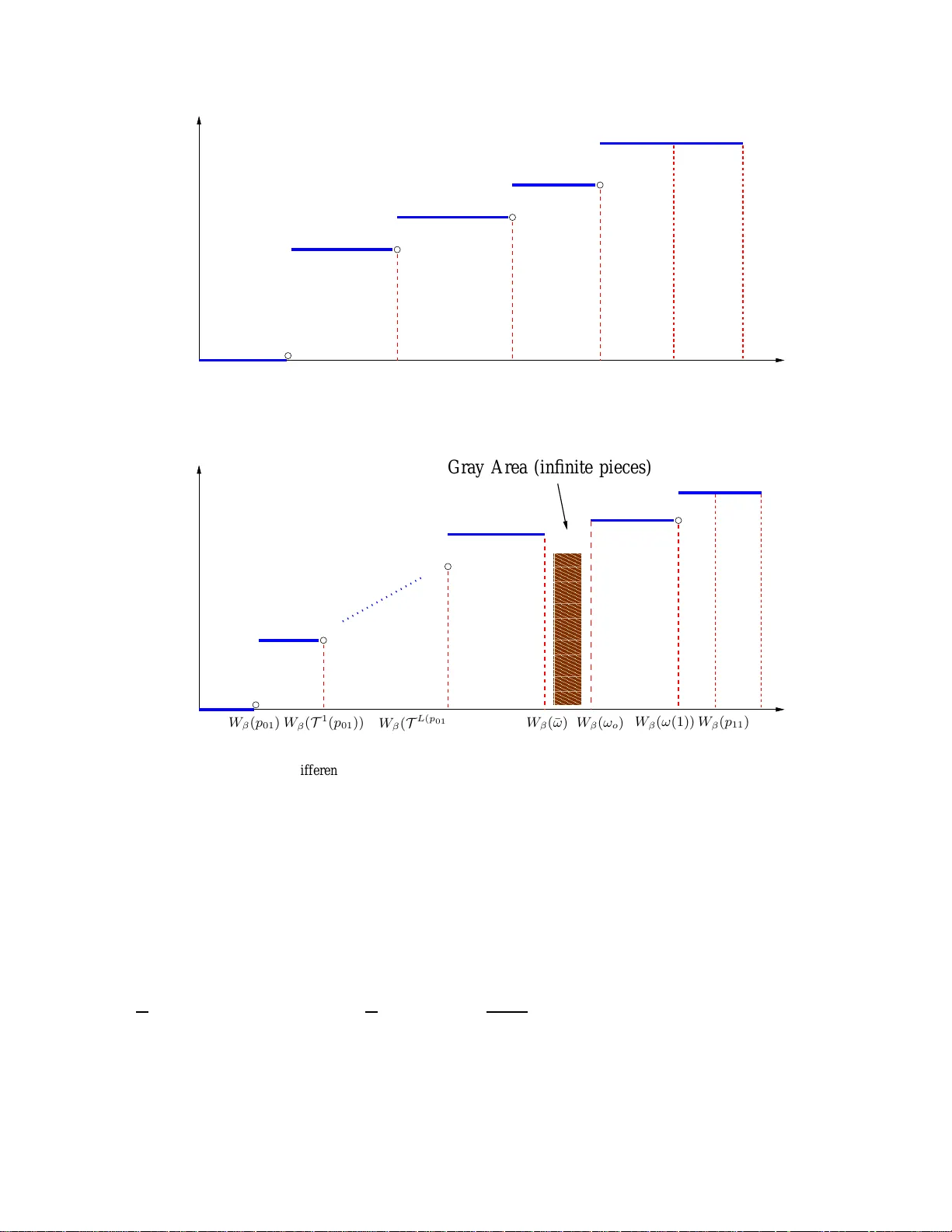
Indexability of Restless Bandit Problems and Optimality of Whittles Index for Dynamic Multichannel Access

Original Paper

Comments & Academic Discussion

Leave a Comment

Original Paper

Related Papers

Comments & Academic Discussion

Leave a Comment