On the Cramer-Rao Lower Bound for Spatial Correlation Matrices of Doubly Selective Fading Channels for MIMO OFDM Systems

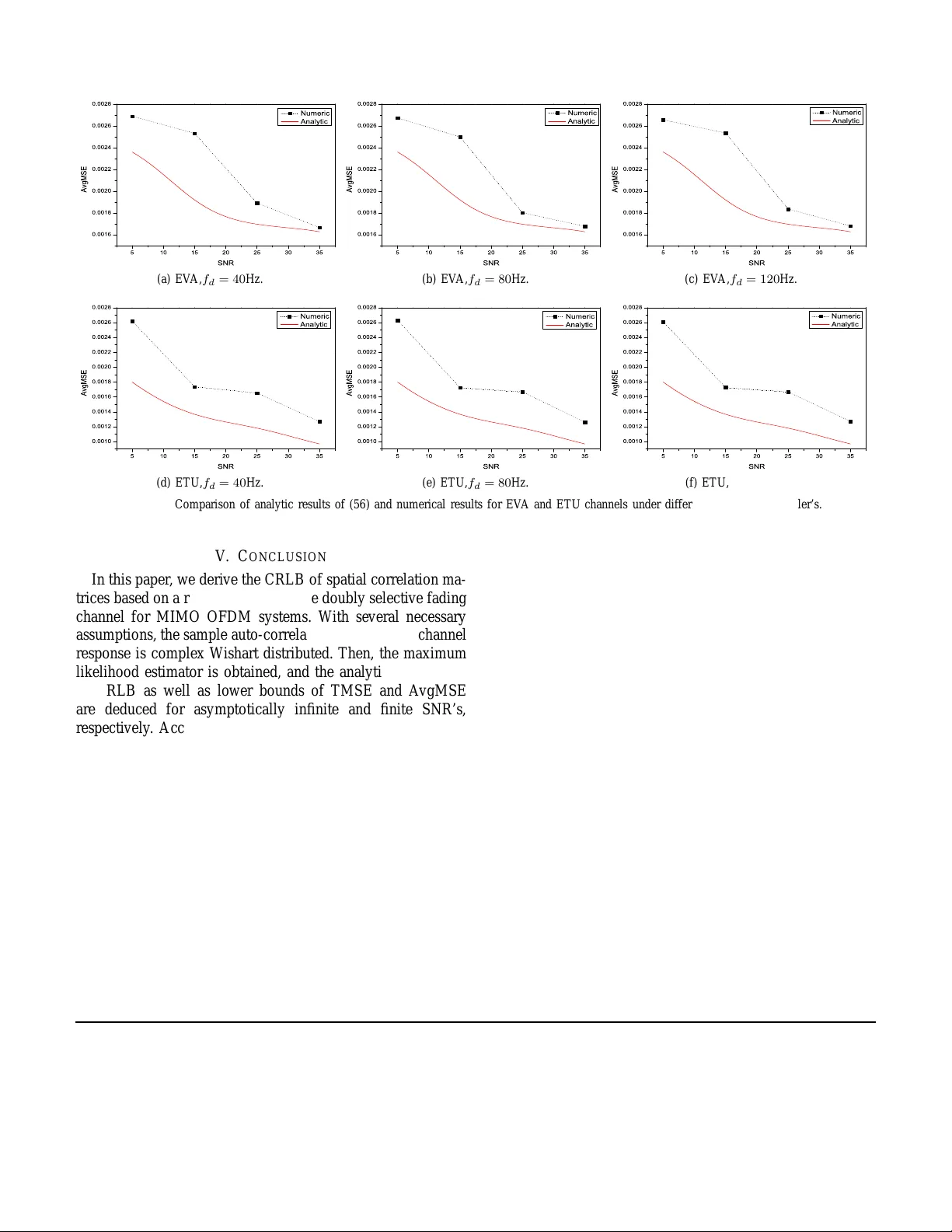
On the Cram ´ er -Rao Lo wer Bound for Spatial Correlati on Matric es of Doub ly Sel ecti v e Fading Channels for MIMO OFDM Systems Xiaochuan Zhao, T ao Peng, Ming Y ang and W enbo W ang W ireless S ignal Processing and Network Lab Ke y Lab oratory of Uni versal W ireless Comm unication, Min istry o f Education Beijing University of Po sts and T elecommunicatio ns, Beijing, China Email: zhaox iaochuan @gmail.com Abstract —In this paper , the Cram ´ er -Rao lower b ound (CRLB) fo r spatial correla tion matrices is deriv ed based on a rigorous model of the doubly selectiv e fading channel fo r mul tiple-inpu t multiple-outp ut (MIMO) orthogonal frequency division mult i- plexing (OFDM ) systems. Adopting an orthogonal pilot p attern fo r mult iple transmitti ng antennas and assuming in dependent samples along the time, the sample auto-corr elation matrix of the channel response is complex Wishart distributed. Th en, the maximum likelihood estimator (MLE) and the a nalytic expr ession of CRLB are derived by assuming that temporal and frequency correla tions are known. Furth ermor e, lower bounds of total mean squ ared error (TMS E) an d av erage mean squared error (A vgMSE) are deduced from CRLB for asymptotically infinite and finite signal-to-noise ratios (S NR’ s), respectively . Accordin g to the lower bound of A vgMSE, th e amount of samples and the order of frequency selectivity show dominant impact on the accuracy of estimation. Besides, the number of pi lot t ones, SNR and normalized maximum Doppler spread together i nfluence th e effectiv e order of frequency selectiv ity . Nu merical simulations demonstrate the analytic results. Index T erms —CRLB, Sp atial correla tion matrices, Dou bly selectiv e fading ch annels, MIMO, OFDM , Complex Wishart. I . I N T RO D U C T I O N Due to the v irtues of o rthogon al f requency division m ul- tiplexing (OFDM) for c on verting frequency selectiv e fading channels into flat fading ones and of multiple-in put mu ltiple- output (MIM O) techniqu es for exploiting spatial di versity gain and/or enhan cing the system cap acity , many current systems combine them two togeth er to achieve a b etter qu ality as well as a higher through put [1]. For M IMO systems, the spatial c orrelation matrices play very imp ortant roles and are wide ly utilized, for exam ple, to facilitate the transmitting precodin g [2] [3], MMSE receiver [4] an d multi-u ser strategies [5 ]. Howe ver , since the tru e spatial cor relation matrices are unk nown in real applicatio ns, the samp le co rrelation matrices have to be used in stead and are usually obtained through the channel estimation. This w ork is sponsore d in part by the National Natural Science Foundat ion of China under grant No.60572120 and 60602058, and in part by the national high technolo gy researching and dev elopin g program of China (National 863 Program) under grant No.2006AA01Z257 and by the National Basic Research Program of China (Nationa l 973 Program) under grant No.2007CB31060 2. In this paper , we study the Cra m ´ er-Rao lo wer bou nd (CRLB) f or the sample spatial correlatio n matrices of do u- bly selecti ve fading chan nels for MIMO OFDM systems. Based o n the a rigorous dou bly fading chan nel mo del and assuming in variant p ilot seq uence along the time, the maxi- mum likelihood estimator (ML E) and the CRLB are der i ved. Then, the analytic expression s of lower bo unds of the total mean squar ed error (TMSE) and av erage mean squar ed error (A vgMSE) are obtained for asymptotically infinite and fin ite signal-to-n oise ratios (SNR’ s), respectively . Based on t he lo wer bound o f A vgMSE, several factors influencing the accuracy of estimation, includin g the amo unt o f samples, the order of frequen cy selectivity , the no rmalized maximum Doppler spread, the number of pilo t tones per antenna and SNR, are further analyzed. This p aper is organized as follows. In Sectio n II, the MI MO OFDM system and chan nel mod el are in troduce d. Then, in Section III, CRLB of the sample spatial co rrelation matrix is derived and furthe r lo wer bounded to uncover the essential fac- tors. Numeric al results ap pear in Section IV. Finally , Section V conclud es the paper . Notation : Lowercase and up percase boldface letters denote column vectors and matrice s, respe cti vely . ( · ) ∗ , ( · ) T , ( · ) H , ( · ) † , and || · || F denote co njugate, transpo sition, conju gate transposition, Moor e-Penrose p seudo-inverse and Frobeniu s norm, respecti vely . ⊗ denotes the Kronecker pr oduct. E ( · ) represents expectation . [ A ] i,j and [ a ] i denotes the ( i , j ) -th element o f A and the i -th eleme nt of a , respectively . diag ( a ) is a diagonal matrix by placing a on the d iagonal. I I . S Y S T E M M O D E L Consider an MIMO OFDM system with a b andwidth of B W = 1 / T Hz ( T is th e sampling period). N d enotes the total n umber of tones, and a cyclic p refix (CP) of length L cp is inserted bef ore each symbol to eliminate inter-block inter- ference. Th us the whole sy mbol d uration is T s = ( N + L cp ) T . Then, n T transmitting anten nas at the base station (BS) and n R receiving antennas at the mobile station (MS) are assumed, respectively . Between the i -th transmitting antenna and j -th receiving antenna, the complex b aseband mo del o f a linear time- variant mobile channe l with L ( j,i ) paths can b e described by [6] h ( j,i ) ( t, τ ) = L ( j,i ) X l =1 h ( j,i ) l ( t ) δ  τ − τ ( j,i ) l T  (1) where ( τ l ) ( j,i ) ∈ R is the normalize d no n-sample-sp aced delay of the l -th p ath, and h ( j,i ) l ( t ) is the correspon ding complex am plitude with th e p ower ( σ 2 l ) ( j,i ) . The following conditio ns are assumed to character ize the correlation prop erty of the chann el. 1) Space Correlation : th e stochastic MIMO rad io channel model [7] is adopted ; 2) Frequen cy Cor relation: the wid e-sense stationary uncor- related scattering (WSSUS) [6] is assumed; 3) T ime Correlation: the uniform scatter ing en vironmen t introdu ced by Clarke [8] is assum ed. 4) Scattering Function Sep arability: th e chan nel h as degen- eracy in all three dimen sions [ 9]. Therefo re, the comp lete spa tial correlation m atrix of the MIMO radio channel is given b y [ 7] Ξ s = Ξ s,T ⊗ Ξ s,R (2) where Ξ s,T ∈ C n T × n T and Ξ s,R ∈ C n R × n R are the sym- metrical complex co rrelation matrices of antenn a arr ays o f BS and MS, respecti vely . Then, th e n ormalized time c orrelation function of any p ath is iden tical, i. e., [ 8] r t (∆ t ) = J 0 (2 π f d ∆ t ) (3) where f d is the maximu m Dop pler spread, and J 0 ( · ) is the zeroth order Bessel function of the first kin d. In addition , L ( j,i ) = L , ( τ l ) ( j,i ) = τ l and ( σ 2 l ) ( j,i ) = σ 2 l , hence, the frequen cy co rrelation matr ix is R f = F τ DF H τ (4) where D = diag ( σ 2 l ) , l = 1 , . . . , L and F τ ∈ C N × L is the unbalan ced F ourier transform matrix, defin ed as [ F τ ] k,l = e − j 2 π kτ l / N . M oreover , the power of the ch annel be tween eac h pair o f transmitting and receiving antennas is nor malized, i.e., tr ( D ) = 1 . Assuming a sufficient CP , i.e ., L cp ≥ L , the d iscrete signal model in the freque ncy dom ain is written as y ( j ) f ( n ) = n T X i =1 H ( j,i ) f ( n ) x ( i ) f ( n ) + n ( j ) f ( n ) (5) where x ( i ) f ( n ) , y ( j ) f ( n ) , n ( j ) f ( n ) ∈ C N × 1 are the n - th trans- mitted and received signal and additive white Gaussian n oise (A WGN) vectors, respectively , an d H ( j,i ) f ( n ) ∈ C N × N is the channel transfer matrix between the i -th transmittin g and j -th receiving antenn as with the ( k + ν, k ) - th elem ent as h H ( j,i ) f ( n ) i k + υ ,k = 1 N N − 1 X m =0 L X l =1 h ( j,i ) l ( n, m ) e − j 2 π ( υ m + kτ l ) / N (6) where h ( j,i ) l ( n, m ) = h ( j,i ) l ( nT s + ( L cp + m ) T ) is the samp led complex amplitude of the l -th path . k and υ de note freq uency and Doppler spread, r espectively . I I I . C R L B O F S PA T I A L C O R R E L A T I O N M A T R I C E S Usually the co rrelation matrices o f th e ch annel r esponse ar e obtained throug h th e least squar ed (LS) channe l estimation on pilot tones, that is, only p ilot symbols ar e extracted and used to p erform LS channel estimation. Therefo re, h ( j,i ) f ,ls ( n ) = ( X ( i ) f ( n )) − 1 y ( j ) f ( n ) (7) where X ( i ) f ( n ) = diag ( x ( i ) f ( n )) is a diagon al matrix co nsist- ing of pilo t sym bols. T o alleviate the in terference b etween multiple transmitting an tennas, p ilot symbols, i.e., x ( i ) f ( n ) , i = 1 , . . . , n T , are designed to be ortho gonal, therefor e ( x ( i 1 ) f ( n )) H x ( i 2 ) f ( n ) = δ ( i 1 − i 2 ) | x ( i 1 ) f ( n ) | 2 2 (8) In th is pape r , we ado pt th e freq uency di vision pilot pattern of wh ich the pilot to nes allocated to a certain transmitting antenna is exclusive o f the others. T o be m ore sp ecifically , it is assumed that th e pilot tone set of the i -th transmitting antenna is I ( i ) p = { i + k × θ ; k = 0 , . . . , P − 1 } , wh ere P is the number of pilot tones of each antenn a satisfy ing L ≤ P , θ ≥ n T and P θ ≤ N . T hus, the i -th transmitting an tenna transmits non-ze ro pilots on I ( i ) p while nulls o n the r est. Besides, we assume that the n on-zero elements of x ( i ) f ( n ) constitute a fixed vector x p ∈ C P × 1 , wh ich is indepen dent of n and i an d of the no rmalized power so that X p X H p = I P , wh ere X p = diag ( x p ) . Then, by discarding the zero elemen ts, ( 7) is further rewritten into h ( j,i ) p,ls ( n ) = X − 1 p H ( j,i ) p ( n ) x p + X − 1 p n ( j,i ) p ( n ) (9) where the subscript p denotes elements on pilot tones. According to th e or thogon al pilot pattern, the instan ta- neous channel imp ulse respo nse (CIR) vector b etween the i - th transm itting antenna an d the j -th recei ving anten na cor- respond ing to th e ( i + k × θ ) -th samp le of the n -th OFDM symbol can be denoted as h ( j,i ) t ( n, i + k × θ ) = [ h ( j,i ) 1 ( n, i + k × θ ) , . . . , h ( j,i ) L ( n, i + k × θ )] T , k = 0 , . . . , P − 1 . Then , the ( j, i ) -th CIR matrix fo r th e n -th OFDM symbol is formed as H ( j,i ) t ( n ) = [ h ( j,i ) t ( n, i ) , . . . , h ( j,i ) t ( n, i + ( P − 1 ) × θ )] . Ac- cording to the assumption s of WSSUS an d u niform scattering , H ( j,i ) t ( n ) is complex n ormal, i.e., H ( j,i ) t ( n ) ∼ C N L × P (0 , Ω ⊗ D ) (10) where Ω ∈ C P × P is a T oeplitz matr ix, defin ed a s [ Ω ] k 1 ,k 2 = J 0 (2 π f d ( k 1 − k 2 ) θT ) (11) Then according to (6) and the pilot pattern, the ( j, i ) -th channel transfer m atrix is H ( j,i ) p ( n ) = F ( i ) τ H ( i ) t ( n ) , where F ( i ) τ is the subm atrix of F τ by drawing rows f rom I ( i ) p . Thus H ( j,i ) p ( n ) ∼ C N P × P (0 , Ω ⊗ [ F ( i ) τ D ( F ( i ) τ ) H ]) (12) Assuming CIR is indepen dent of the therma l n oise, with (9) and (12), we have h ( j,i ) p,ls ( n ) ∼ C N P (0 , Υ ( j,i ) ) (13) where the cov ariance m atrix Υ ( j,i ) is defined as Υ ( j,i ) = ( x H p Ωx p )( X H p F ( i ) τ D ( F ( i ) τ ) H X p ) + σ 2 n I P (14) Apparen tly , Υ ( j,i ) is irr elev an t of the in dexes o f the receiving antennas, wh ich follows the assump tion 4). Ac cording to the orthog onal pilo t pattern, F ( i ) τ = F (0) τ Φ i , wher e F (0) τ ∈ C P × L is a submatrix of F τ by d rawing rows from I (0) p = { k × θ ; k = 0 , . . . , P − 1 } and Φ is a diagon al ph ase-twisted matrix with [ Φ ] l,l = e − j 2 π τ l / N . Then , the fre quency auto -correlation matrix of I ( i ) p is R ( i ) p = F ( i ) τ D ( F ( i ) τ ) H = F (0) τ Φ i D ( F (0) τ Φ i ) H = R p (15) where R p = F (0) τ D ( F (0) τ ) H . Furth ermore, to simplify the following d eriv ation , we assume that CFR v aries slightly within n T contiguo us tones, so th at the fre quency cro ss- correlation matrix between the pilot sets I ( i 1 ) p and I ( i 2 ) p is R ( i 1 ,i 2 ) p = F ( i 1 ) τ D ( F ( i 2 ) τ ) H = F (0) τ Φ i 1 − i 2 D ( F (0) τ ) H ≈ R p (16) Then, the complete LS-estimated channel transfer matrix is constructed as H p,ls ( n ) =      h (1 , 1) p,ls ( n ) · · · h (1 ,n T ) p,ls ( n ) . . . . . . . . . h ( n R , 1) p,ls ( n ) · · · h ( n R ,n T ) p,ls ( n )      P n R × n T (17) and it is complex nor mal, i.e., H p,ls ( n ) ∼ C N P n R × n T (0 , Σ ) (18) where Σ ∈ C P n R n T × P n R n T . Acco rding to the assumption s 1)-4), its (( i 1 − 1 ) n R + j 1 , ( i 2 − 1 ) n R + j 2 ) -th submatrix is (19), shown at b ottom of the next pag e. Then, with (15) and (16), Σ is expressed as Σ = Ξ s ⊗ ( ω A ) + σ 2 n I n T n R P (20) where ω = x H p Ωx p and A = X H p R p X p . When N t complete LS estimated ch annel tr ansfer matrices are a vailable, the sample auto- correlation matrix is for med as ˆ Σ = 1 N t N t X n =1 vec ( H p,ls ( n )) vec ( H p,ls ( n )) H (21) where N t is the nu mber of samp les. T o d eriv e the probab ility density fu nction (PDF) of the sample auto- correlation matrix, we assume that samples are ind ependen t o f each other, wh ich may be a strict constraint. Howe ver, whe n the spacing between two contiguo us pilot sym bols is sufficiently large, the co rre- lation between them is rath er low , which alleviates the effect of m odel mismatch . Then, ˆ Σ has the co mplex central Wis hart distribution with N t degrees of freed om and covariance matrix Σ ′ = Σ /N t [10], denoted as ˆ Σ ∼ C W n T n R P ( N t , Σ ′ ) (22) and its PDF is f ( ˆ Σ ) = etr ( − Σ ′− 1 ˆ Σ )[det( ˆ Σ )] N t − n T n R P C Γ n T n R P ( N t )[det( Σ ′ )] N t (23) where etr ( · ) = ex p( tr ( · )) a nd C Γ n T n R P ( N t ) is the complex multiv a riate gamm a functio n, defin ed as C Γ n T n R P ( N t ) = π n T n R P ( n T n R P − 1) / 2 n T n R P Y k =1 Γ( N t − k + 1) Then, according to (23), the likelihood func tion with respect to th e parameter matrix Ξ s can be written as L ( Ξ s ) = tr ( − Σ ′− 1 ˆ Σ ) + ( N t − n T n R P ) ln(det( ˆ Σ )) − ln( C Γ n T n R P ( N t )) − N t ln(det( Σ ′ )) (24) Therefo re, the score functio n [11] is score ( vec ( Ξ s )) = ∂ L ( Ξ s ) ∂ vec ( Ξ s ) = ∂ vec ( Σ ′ ) T ∂ vec ( Ξ s ) ∂ L ( Ξ s ) ∂ vec ( Σ ′ ) (25) where the first multip licati ve term on the r ight-han d side, accordin g to (20), is ∂ vec ( Σ ′ ) T ∂ vec ( Ξ s ) = ω N t ∂ vec ( Ξ s ⊗ A ) T ∂ vec ( Ξ s ) (26) and the second term is ∂ L ( Ξ s ) ∂ vec ( Σ ′ ) = vec [( Σ ′− 1 ˆ ΣΣ ′− 1 − N t Σ ′− 1 ) T ] (27) Since vec ( Ξ s ⊗ A ) = K ⊗ [ vec ( Ξ s ) ⊗ vec ( A ) ] (28) where K ⊗ is K ⊗ = I n R n T ⊗ K T ( n R n T ) P ⊗ I P (29) where K ( n R n T ) P ∈ R ( n R n T ) P × ( n R n T ) P is a transpose ma- trix satisfying vec ( B T ) = K ( n R n T ) P vec ( B ) , where B ∈ C n R n T × P . Hen ce, (26) is rewritten into ∂ vec ( Σ ′ ) T ∂ vec ( Ξ s ) = ω N t [ I ( n R n T ) 2 ⊗ vec ( A ) T ] K T ⊗ (30) By letting the score function equal zero, we know that the maximum lik elihood estimator (MLE) of Σ is ˆ Σ , so, with (1 9), its ( k 1 , k 2 ) -th submatrix, denoted as { Σ } ( P × P ) k 1 ,k 2 ∈ C P × P , ca n be used to estimate [ Ξ s ] k 1 ,k 2 by [ Ξ s ] k 1 ,k 2 × ( ω A k 1 ,k 2 ) + σ 2 n δ ( k 1 − k 2 ) I P = { Σ } ( P × P ) k 1 ,k 2 (31) where k 1 = ( i 1 − 1) n R + j 1 , k 2 = ( i 2 − 1) n R + j 2 , and A k 1 ,k 2 = X H p R ( i 1 ,i 2 ) p X p (32) Note that A k 1 ,k 2 and σ 2 n are assumed to be kn own for (31), that is, the frequen cy auto/c ross-correlatio n ma trices, the pilot sequence and the noise power a re available. In order to solve [ Ξ s ] k 1 ,k 2 from (31), th e singular matrices of A k 1 ,k 2 , denoted as U k 1 ,k 2 and V k 1 ,k 2 , is used to transform (31) into ω [ Ξ s ] k 1 ,k 2 Λ k 1 ,k 2 + σ 2 n δ ( k 1 − k 2 ) I P = U H k 1 ,k 2 { Σ } ( P × P ) k 1 ,k 2 V k 1 ,k 2 where Λ k 1 ,k 2 is a diag onal matrix with sing ular values of A k 1 ,k 2 on the diag onal. Th en, sin ce ran k ( A k 1 ,k 2 ) = rank ( R p ) = L , the MLE of [ Ξ s ] k 1 ,k 2 is MLE ([ Ξ s ] k 1 ,k 2 ) = L X l =1 c l [ U H k 1 ,k 2 { Σ } ( P × P ) k 1 ,k 2 V k 1 ,k 2 ] l,l − σ 2 n δ ( k 1 − k 2 ) [ Λ k 1 ,k 2 ] l,l (33) where c l ’ s are norma lized non-n egati ve weight co efficients, i.e., c l ≥ 0 an d P L l =1 c l = 1 . Further, according to the score function , the Fisher In for- mation matrix with respect to Ξ s [11] is J ( Ξ s ) = E "  ∂ L ( Ξ s ) ∂ vec ( Ξ s )   ∂ L ( Ξ s ) ∂ vec ( Ξ s )  H # (34) with (25)( 30)(27), (34) is rewritten into (35), sho wn at the bottom of the next page, where B = Σ ′− 1 ˆ ΣΣ ′− 1 . Notice that B ∼ C W N ( N t , Σ ′− 1 ) therefor e E { vec [( B − N t Σ ′− 1 ) T ] vec [( B − N t Σ ′− 1 ) T ] H } = V ar [ vec ( B T )] (36) According to [12], (36) is V ar [ vec ( B T )] = N t ( Σ ′− H ⊗ Σ ′− T ) (37) Then, with (37), J ( Ξ s ) is J ( Ξ s ) = ω 2 N t [ I ( n R n T ) 2 ⊗ vec ( A k 1 ,k 2 ) T ] K T ⊗ ( Σ ′− H ⊗ Σ ′− T ) × K ⊗ [ I ( n R n T ) 2 ⊗ vec ( A k 1 ,k 2 ) ∗ ] (38) Therefo re, the CRLB of Ξ s is [11] CRLB ( Ξ s ) = J − 1 ( Ξ s ) (39) Now we consider the case that the SNR is asy mptotically infinite, o r , equiv alently , the p ower of no ise is zero. Accordin g to (20), then, Σ ′ is reduced to Σ ′ = ω N t Ξ s ⊗ A (40) Since A is ran k deficien t if L < P , Σ ′− 1 should be re placed by Σ ′† . Then K T ⊗ ( Σ ′† H ⊗ Σ ′† T ) K ⊗ = N 2 t ω 2 Ξ − H s ⊗ Ξ − T s ⊗ A † H ⊗ A † T (41) W ith (4 1), ( 38) is rewritten into J ( Ξ s ) = N t [ I ( n R n T ) 2 ⊗ vec ( A ) T ][( Ξ − H s ⊗ Ξ − T s ) ⊗ ( A † H ⊗ A † T )][ I ( n R n T ) 2 ⊗ vec ( A ) ∗ ] = αN t ( Ξ − H s ⊗ Ξ − T s ) (42) where α = vec ( A ) T ( A † H ⊗ A † T ) vec ( A ) ∗ = L (43) From (42) and (43), (39) is rewritten into CRLB ( Ξ s ) = 1 LN t ( Ξ H s ⊗ Ξ T s ) (44) Based on (44), a lower boun d of T MSE o f estimating Ξ s is obtained, i.e., TMSE LB ( Ξ s ) = tr [ CRLB ( Ξ s )] = ( n T n R ) 2 LN t (45) And, accordin gly , th e lower bound of A vg MSE o f Ξ s is A v gMSE LB ( Ξ s ) = TMSE LB ( Ξ s ) ( n T n R ) 2 = 1 LN t (46) In rea l application s, the numb er of sign ificant eigenv alue s of A , denoted as L s , may be less than L . Sin ce the amount of samples, N t , is finite, the in significant eigen values are much less cred ible than significant on es. Theref ore, only sign ificant ones ar e used in (33). Besides, the weig hts of significant ones are considered to be equal. Hence, ( 33) is changed into MLE ([ Ξ s ] k 1 ,k 2 ) = L s X l =1 [ U H k 1 ,k 2 { Σ } ( P × P ) k 1 ,k 2 V k 1 ,k 2 ] l,l − σ 2 n δ ( k 1 − k 2 ) L s [ Λ k 1 ,k 2 ] l,l (47) Correspon dingly , the lower bou nd of a verage MSE of Ξ is modified into A v gMSE LB ( Ξ s ) = 1 αN t = 1 L s N t (48) In fact, L s represents the ord er of frequen cy selectivity , that is, the number of equ iv alen t in depend ent p arallel transmission branch es of the multipath channels for OFDM systems. When the SNR is finite, Σ ′ is appro ximated as Σ ′ = ω N t Ξ s ⊗ ( A + σ 2 n ω I P ) (49) and, co rrespon dingly , ( 39) is rewritten into CRLB ( Ξ s ) = 1 β N t ( Ξ H s ⊗ Ξ T s ) (50) and (46) is rewritten into A v gMSE LB ( Ξ s ) = 1 β N t (51) { Σ } ( P × P ) ( i 1 − 1) n R + j 1 , ( i 2 − 1) n R + j 2 = [ Ξ s ] ( i 1 − 1) n R + j 1 , ( i 2 − 1) n R + j 2 × ( ω X H p R ( i 1 ,i 2 ) p X p ) + σ 2 n δ ( i 1 − i 2 ) δ ( j 1 − j 2 ) I P (19) where β = vec ( A ) T [( A + σ 2 n ω I P ) − H ⊗ ( A + σ 2 n ω I P ) − T ] vec ( A ) ∗ = L X l =1 [ 1 1 + ( ω ρ l ) − 1 ] 2 (52) where ρ l = λ l σ 2 n and λ l is the l -th eigenv alu e of A . Moreover , since ω = x H p Ωx p = k x p k 2 2 × x H p Ωx p x H p x p = k x p k 2 2 × R ( Ω ) (53) where k x p k 2 2 is the power of p ilot symbol, and R ( Ω ) is the Rayleigh quotien t of Ω [13 ]. D ue to the normalized power , k x p k 2 2 = P . Besides, it is straightforward that R ( Ω ) ≤ λ max ( Ω ) , wh ere λ max ( Ω ) denotes the m aximum eig en value of Ω . Acco rding to [14 ], when θ f d T s ≤ 0 . 35 , λ max ( Ω ) can be well approxim ated by λ max ( Ω ) ≈ P J 0 (2 π cθ f d T s ) (54) where c = 0 . 35 . Ther efore, β is upper b ounded by β ≤ L X l =1 [ 1 1 + ( P 2 J 0 (2 π cθ f d T s ) ρ l ) − 1 ] 2 = β max (55) Then, (51) is further lower boun ded by A v gMSE LB ( Ξ s ) = 1 β max N t (56) Note that ω ρ l can be regarded as th e effective SNR on the l -th subchann el. When ω ρ l is too small, say , below 0 dB, it sho uld not be used in MLE (47), which would re duce the effective order o f freque ncy selecti v ity . Acco rding to (55), th erefore, the number o f p ilot to nes, SNR a nd m aximum Doppler spr ead together in fluence the ef fective orde r of f requency selecti vity and, further, th e accuracy of estimation . I V . N U M E R I C A L R E S U LT S The OFDM system in simulations is of B W = 1 . 25 MH z ( T = 1 /B W = 800 ns), N = 128 , and L cp = 16 . T wo 3 GPP E-UTRA channe l m odels are adopted : Exten ded V ehicu lar A mo del (EV A) an d Extend ed T ypical U rban mo del (ETU) [15]. The excess tap delay of EV A is [ 0 , 3 0 , 150 , 310 , 3 70 , 710 , 109 0 , 1730 , 2510 ] ns, and its relativ e power is [ 0 . 0 , − 1 . 5 , − 1 . 4 , − 3 . 6 , − 0 . 6 , − 9 . 1 , − 7 . 0 , − 1 2 . 0 , − 16 . 9 ] dB. For ETU, they are [ 0 , 50 , 12 0 , 200 , 230 , 500 , 1600 , 2 300 , 5000 ] n s and [ − 1 . 0 , − 1 . 0 , − 1 . 0 , 0 . 0 , 0 . 0 , 0 . 0 , − 3 . 0 , − 5 . 0 , − 7 . 0 ] dB, respectively . The classic Doppler spectrum, i.e., Jakes’ spectrum [6], is applied to g enerate the Rayleigh fadin g channel. Th e M IMO co nfiguratio n is 4 × 4 , and the c orrelation matrices o f transmittin g and recei ving anten nas are shown at the bottom o f the n ext page, respectively [ 7]. Besides, the 2 0 0 4 0 0 6 0 0 8 0 0 1 0 0 0 0 . 0 0 0 0 . 0 0 1 0 . 0 0 2 0 . 0 0 3 0 . 0 0 4 0 . 0 0 5 A vg M S E A m o u n t o f S a m p l e s L s= 1 , N u m e r i ca l L s= 2 , N u m e r i ca l L s= 3 , N u m e r i ca l L s= 4 , N u m e r i ca l L s= 5 , N u m e r i ca l L s= 1 , A n a l y t i ca l L s= 2 , A n a l y t i ca l L s= 3 , A n a l y t i ca l L s= 4 , A n a l y t i ca l L s= 5 , A n a l y t i ca l (a) E V A 2 0 0 4 0 0 6 0 0 8 0 0 1 0 0 0 0 . 0 0 0 0 . 0 0 1 0 . 0 0 2 0 . 0 0 3 0 . 0 0 4 0 . 0 0 5 A vg M S E A m o u n t o f S a m p l e s L s= 1 , N u m e r i ca l L s= 2 , N u m e r i ca l L s= 3 , N u m e r i ca l L s= 4 , N u m e r i ca l L s= 5 , N u m e r i ca l L s= 1 , A n a l y t i ca l L s= 2 , A n a l y t i ca l L s= 3 , A n a l y t i ca l L s= 4 , A n a l y t i ca l L s= 5 , A n a l y t i ca l (b) ETU Fig. 1. Compa rison of analytic results of (48) and numerical results for EV A and E TU channels when S N R → ∞ and f d = 100 Hz. number of p ilot tones p er transmitting an tenna is 16, th e pilot spacing is 8, an d the p ilot symbols ar e separated far en ough from others to reduce the correlation am ong them. In Fig.1, we comp are the a nalytic results (48) and the numerical results over a rang e o f N t ’ s for EV A and ETU channels, respectively , when the SNR is asymptotically infinite and f d = 100 Hz. Th e pilot sequences ar e QPSK m odulated and randomly chosen. Besides, dif ferent L s ’ s are tested to demonstra te that (48) is a tight lower bo und of ( 47). Appar- ently , the analytic r esults meet the n umerical one s quite well. In Fig .2, different SNR’ s and maxim um Dopp ler spread s are tested to demo nstrate that ( 56) is tigh t lower b ound of (47) when the pilot sequence, x p , is pr operly selected, spe cifically , the eigenv ector of Ω associated with the maxim um eigen value. Since the num ber of p ilot to nes, SNR and n ormalized max - imum Doppler spread tog ether influence the effecti ve orde r of frequen cy selecti v ity , the value of L s varies fo r d ifferent cases, which is reflecte d by varying A vgMSE. Further, it is obvious that SNR h as a more significant imp act on L s than the maximum Do ppler sp read, wh en the n umber o f p ilot tones are large eno ugh, e.g. , over 1 6. J ( Ξ s ) = ω 2 N 2 t [ I ( n R n T ) 2 ⊗ vec ( A ) T ] K T ⊗ E { vec [( B − N t Σ ′− 1 ) T ] vec [( B − N t Σ ′− 1 ) T ] H } K ⊗ [ I ( n R n T ) 2 ⊗ vec ( A ) ∗ ] (35) 5 1 0 1 5 2 0 2 5 3 0 3 5 0 . 0 0 1 6 0 . 0 0 1 8 0 . 0 0 2 0 0 . 0 0 2 2 0 . 0 0 2 4 0 . 0 0 2 6 0 . 0 0 2 8 A vg M S E S N R N u m e r i c A n a l y t i c (a) E V A, f d = 40 Hz. 5 1 0 1 5 2 0 2 5 3 0 3 5 0 . 0 0 1 6 0 . 0 0 1 8 0 . 0 0 2 0 0 . 0 0 2 2 0 . 0 0 2 4 0 . 0 0 2 6 0 . 0 0 2 8 A vg M S E S N R N u m e r i c A n a l y t i c (b) EV A, f d = 80 Hz. 5 1 0 1 5 2 0 2 5 3 0 3 5 0 . 0 0 1 6 0 . 0 0 1 8 0 . 0 0 2 0 0 . 0 0 2 2 0 . 0 0 2 4 0 . 0 0 2 6 0 . 0 0 2 8 A vg M S E S N R N u m e r i c A n a l y t i c (c) E V A, f d = 120 Hz. 5 1 0 1 5 2 0 2 5 3 0 3 5 0 . 0 0 1 0 0 . 0 0 1 2 0 . 0 0 1 4 0 . 0 0 1 6 0 . 0 0 1 8 0 . 0 0 2 0 0 . 0 0 2 2 0 . 0 0 2 4 0 . 0 0 2 6 0 . 0 0 2 8 A vg M S E S N R N u m e r i c A n a l y t i c (d) ETU, f d = 40 Hz. 5 1 0 1 5 2 0 2 5 3 0 3 5 0 . 0 0 1 0 0 . 0 0 1 2 0 . 0 0 1 4 0 . 0 0 1 6 0 . 0 0 1 8 0 . 0 0 2 0 0 . 0 0 2 2 0 . 0 0 2 4 0 . 0 0 2 6 0 . 0 0 2 8 A vg M S E S N R N u m e r i c A n a l y t i c (e) E TU, f d = 80 Hz. 5 1 0 1 5 2 0 2 5 3 0 3 5 0 . 0 0 1 0 0 . 0 0 1 2 0 . 0 0 1 4 0 . 0 0 1 6 0 . 0 0 1 8 0 . 0 0 2 0 0 . 0 0 2 2 0 . 0 0 2 4 0 . 0 0 2 6 0 . 0 0 2 8 A vg M S E S N R N u m e r i c A n a l y t i c (f) ET U, f d = 120 Hz. Fig. 2. Comparison of analytic results of (56) and numerica l results for EV A and ETU channe ls under diffe rent SNR’ s and Doppler’ s. V . C O N C L U S I O N In this paper, we der i ve the CRLB of sp atial cor relation ma- trices based on a r igorou s model of the doub ly selecti ve fading channel f or MIMO O FDM systems. W ith sev eral necessary assumptions, the sample au to-corr elation m atrix of the chan nel response is co mplex W ishart distributed. Then, the max imum likelihood estimator is obtained , and the analytic expre ssions of CRLB as well as lower bou nds of TMSE and A vgMSE are deduced fo r asy mptotically in finite and fin ite SNR’ s, respectively . Accordin g to the lower bou nd of A vgMSE, the amount of samp les an d the ord er of freque ncy selectivity influence the accuracy o f estimatio n d ominantly . Besides, th e number of p ilot tones, SNR and maximum Dopp ler spre ad have effects on the effecti ve order of frequency selectivity . R E F E R E N C E S [1] G. St ¨ uber , J. Barry , S. McLaughli n, Y . Li, M. Ingram, and T . Pratt, “Broadba nd MIMO-OFDM Wirel ess Communica tions, ” Proc eeding of the IEEE , vol. 92, pp. 271–294, February 2004. [2] A. Gorokhov , “Ca pacit y of Mult i-Antenna Rayle igh Channel with a Limited Tra nsmit Di versi ty , ” in IEEE ISIT 00 , Sorrento, Italy , June 2000. [3] H. Sampath and A. Paulraj, “Linear Precoding for Space-T ime Coded Systems with Known Fading Correlati ons, ” in Proc . Asilomar Conf . on Singals, Systems and Computers, 1 , Pacific Grove, CA, Nov ember 2001. [4] A. Nordio and G. T aricco, “Linear Rec ei vers for the Multi ple-Input Multipl e-Output Multiple-Acc ess Channel, ” IE EE T rans. Commun. , vol. 54, pp. 1446–1456, August 2006. [5] E. Jorswieck and H. Boche, “Transmission Strategi es for the MIMO MA C with MMSE Rec ei ver: A verage MSE Optimiz ation and Achie vabl e Indi vidual MSE Region , ” IEEE T rans. Signal Process. , vol. 51, pp. 2872–2881, Nov ember 2003. [6] R. Steele, Mobile Radio Communica tions . IEEE Press, 1992. [7] J. Kermoal , L. Schumacher , K. Pedersen, P . Mogensen, and F . Fred- eriksen, “A Stochastic MIMO Radio Channel Model with Experimental V alidati on, ” IEEE J . Sel. Areas Commun. , vol . 20, pp. 1211–1226, August 2002. [8] R. Clarke, “A Statisti cal Theory of Mobile Radio Rece ption, ” Bell Syst. T ech. J . , pp. 957–1000, July-Auguest 1968. [9] A. Paul raj, R. Nabar , and D. Gore, Introd uction to Space-T ime W ir eless Communicat ions , 1st ed. Cambridge, England: Cambridge Uni versity Press, 2003. [10] T . Ratnaraj ah, R. V aillancourt , and M. Alvo, “Complex Random Ma- trices and Rayleigh Channel Capacity , ” Commun. Inf. Syst. , vol. 3, pp. 119–138, October 2003. [11] K. Mardia, J. Kent , and J. Bib by , Multi variate A nalysis . Academic Press, 1979. [12] D. Ma iwal d and D. Kraus, “Ca lcula tion of Moments of Comple x W ishart and Complex In verse W ishart Distribute d Matric es, ” IEE Pro c.-Radar . Sonar Navig. , vol. 147, pp. 162–168, August 2000. [13] G. Golub and C. V . Loan, Matrix Computat ions , 3rd ed. Ne w Y ork: Johns Hopkins Univ ersity Press, 1996. [14] X. Zhao and M. Y ang and T . Peng and W . W ang, “On the Cram ´ er-Ra o Lowe r Bound for Frequenc y Correlatio n Matric es of Doubly Selecti ve Fadi ng Channel s for O FDM Systems, ” Submitted to IEEE ICC 09 , Dresden, Germany , June 2009. [15] “3GPP TS 36.101 v8.2. 0 – Evolve d Univ ersal Terrestria l Radio Access (E-UTRA); User E quipment (UE) Radio T ransmission and Rece ption (Relasa se 8), ” 3GPP , May 2008. Ξ s,T = Ξ s,R =     1 − 0 . 13 − j 0 . 62 − 0 . 49 + j 0 . 23 0 . 15 + j 0 . 28 − 0 . 13 + j 0 . 62 1 − 0 . 13 − j 0 . 52 − 0 . 38 + j 0 . 12 − 0 . 49 − j 0 . 23 − 0 . 13 + j 0 . 52 1 0 . 02 − j 0 . 61 0 . 15 − j 0 . 28 − 0 . 3 8 − j 0 . 12 0 . 02 + j 0 . 61 1     ,     1 − 0 . 45 + j 0 . 53 0 . 37 − j 0 . 22 0 . 19 + j 0 . 21 − 0 . 45 − j 0 . 53 1 − 0 . 35 − j 0 . 02 0 . 02 − j 0 . 27 0 . 37 + j 0 . 22 − 0 . 35 + j 0 . 02 1 − 0 . 10 + j 0 . 54 0 . 19 − j 0 . 21 0 . 02 + j 0 . 27 − 0 . 10 − j 0 . 54 1    