Quasi-metrics, Similarities and Searches: aspects of geometry of protein datasets

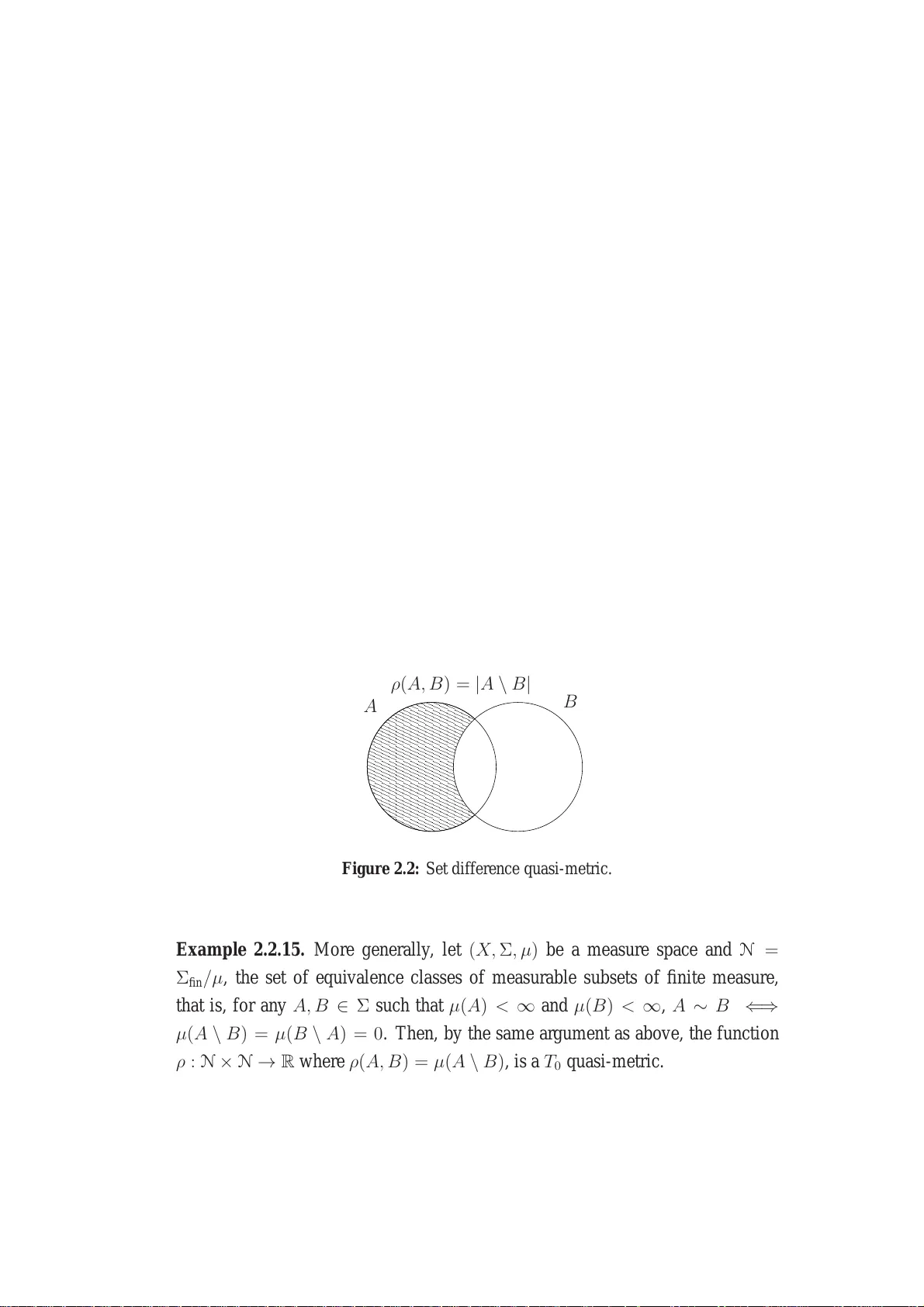
Quasi-metrics, Similarities and Sear ches: aspects of geome try of pr otein datasets by Aleksandar Stojmirovi ´ c A thesis submitted to the V ictoria Univ ersity of W ellington in fulﬁlment of the requirements for the degree of Doctor of Philosophy in Mathematics. V ictoria Univer si ty of W ellington 2005 Abstract A quasi -metric is a di stance function which sat isﬁes the triangl e inequalit y b ut is not symmetric: it can be thought of as an asymmetric metric. Quasi-metrics were ﬁrst i ntroduced in 1930s and are a subject of intensiv e research in th e cont ext of topology and theoretical computer science. The ce ntral result of this thesis, de veloped in C hapter 3, is that a natural corr e- spondence e xis ts between similarity m easures between biological (nucleoti de or protein) sequences and quasi-m etrics. A s sequence sim ilarity search is one of the most important t echniques of m odern bioinformatics, this motiv ates a new direc- tion of research: dev elopment of g eometric aspects of the theory of quasi-metric spaces and its app lications to simi larity search in general and l ar ge protein datasets in particular . The thesis starts by presenting b asic concepts of the th eory of quasi-metri c spaces illustrated b y numerous examples, some previously known, so me novel. In particular , the u niv ersal coun table rational q uasi-metric space and its bi comple- tion, t he unive rsal bicom plete separable quasi-metric space are constructed. Sets of biol ogical sequences with some comm only used simil arity measures provide a further and the most important example. Chapter 4 is d edicated to dev elopm ent of a notion of the quasi-metri c space with Borel probabilit y measure, or pq-sp ace . The concept of a pq -space is a gen- eralisation of a notion of an mm -space from the asympt otic geometric analy sis: an mm -space is a metric space wi th Borel measure th at p rovides the framew ork for study o f t he phenomenon o f concentration of measure on high dimension al structur es . While so me concepts and results are direct e xtensi ons of results about mm -spaces, some are intrinsi c to the quasi-m etric case. One o f t he m ain results of this chapter ind icates th at ‘a high dim ensional quasi -metric s pace i s clo se to being a metric space’. Chapter 5 in vestigates the geometric aspects of the theory of database similar- ity search. It extends the existing conce pts of a workload and an indexing scheme in order to cover more general cases and introduces the concept of a quasi-metric tr ee as an analogue to a metric tree , a popul ar class of access meth ods for met ric datasets. The result s about pq -spaces are used t o produce som e new theoretical bounds on performance of indexing schemes. Finally , the thesis presents some biological applications. Chapter 6 introduces FSIndex, an indexing scheme that s igniﬁcantly accelerates similarity searches of short protein fragment datasets. The performance of FSInde x turns out to be very good in com parison with existing access methods. Chapter 7 presents the prototype of the s ystem for discov ery of short functional protein motifs called PFMFind, which relies on FSIndex for similarity searches. Acknowl edgemen ts I am indebted to man y people and institutions who ha ve helped me to survi ve and e ven enjoy the four years it took to produce this thesis. First of all I wish to off er my sincere st thanks to m y supervisors, Dr . Vladimi r Pestov , who was a Reader in Mathem atics at V ictoria U niv ersity of W ellington when I started my PhD studies and is now a Professor of Mathematics at the Univ ersity of Ottawa, and Dr . Bill Jordan, Reader in Biochem istry at V i ctoria Univ ersity of W ellington, who ha ve suppo rted me and guided me in all im aginable ways during the course of the study . Dr . M ike Boland fr om the Fonterra Research Centre was prin cipal in getting my study off the ground b y int roducing me to th e problem of short peptide fragments. My scholarship stipend was provided through a Bright Future Enterprise Schol- arship joi ntly funded by the The Foundation for Research, Science and T echnol- ogy and Fonterra Research Centre (formerly The New Zealand D airy Research Institute). I ha ve enjoyed a generous and consistent support from the F aculty of Science , the School of Mathemati cal and Computing Sciences and the School of Biological Sciences at the V ictoria University of W ellington. Not only hav e they contrib uted signiﬁcant funds towar ds my t ra vels to conferences and to Canada t o visit my su- pervisor as well as t ow ards a part of tuiti on fees, but hav e provided an excellent en vi ronment to w ork in. I would particularly lik e to thank Dr . Peter Donelan, who was the head of the School of Math ematical and Computing Sciences for most of the time I was doing my thesis and who signed my progress re ports inst ead of my principal supervisor . I am grateful to Professor Estate Khmaladze and Dr . Peter iii iv Andreae for being willing to list en to my num erous quest ions i n their respectiv e areas. I also wish to acknowledge the system programmers Mark Da vis and Dun- can McEwan for maintaini ng our system s and being always av ailable to answer my qu estions about C programming, UNIX, networks etc. I wish t o thank the Department of Mathematics and Statistics of the University of Ottaw a, which has accepted me as a visitor on two occasions for four months in total. I thank m y colleagues Azat Arslanov and T odd Rangiwhetu who at times shared ofﬁ ce with me for encouraging me and proofreading some of my manuscript s. I would like to thank Professor V i tali Mil man who, while bein g a visito r in W ellington, offered a lot of encouragement and some very helpful advice on how to approach math ematics. A very s pecial thanks g oes to Dr . Markus Hegland for con v incing me to l earn the Python p rogramming language and ease m y program- ming burden. Markus was also one of t he supervisors (the oth er bein g Vladimir Pestov) for my summ er 1999 project at t he Australi an National U niv ersity that is presented as Appendix A. Professor Paolo Ciaccia and Dr . Marco Patella have generously made the source code for their M-tree publicly av ailable on the web and hav e agreed to send me a copy of the code for mvp-tree. My mother Lji ljana has supported m e throughout my stu dies and sacriﬁced a lot to see me where I am now . No words can eve r be sufﬁcient to express my gratitude. Contents Abstract i Acknowledgeme nts iii Contents v List of Figure s x List of T ables xii List of Algorithms xiii 1 Intr oduction 1 1.1 Proteins . . . . . . . . . . . . . . . . . . . . . . . . . . . . . . . 2 1.1.1 Basic concepts . . . . . . . . . . . . . . . . . . . . . . . 2 1.1.2 Protein sequence alignment . . . . . . . . . . . . . . . . 4 1.1.3 Short peptide fragments . . . . . . . . . . . . . . . . . . 7 1.2 Indexing for Similarity Search . . . . . . . . . . . . . . . . . . . 8 1.3 Quasi-metrics . . . . . . . . . . . . . . . . . . . . . . . . . . . . 10 1.4 Overvie w of the Chapters . . . . . . . . . . . . . . . . . . . . . . 11 2 Quasi-metric Spaces 15 2.1 Basic Deﬁnitions . . . . . . . . . . . . . . . . . . . . . . . . . . 16 2.2 T opologies and quasi-uniformit ies . . . . . . . . . . . . . . . . . 19 2.3 Quasi-normed Spaces . . . . . . . . . . . . . . . . . . . . . . . . 26 v vi CONTENTS 2.4 Lipschitz Functions . . . . . . . . . . . . . . . . . . . . . . . . . 29 2.4.1 Examples . . . . . . . . . . . . . . . . . . . . . . . . . . 31 2.4.2 Quasi-normed spaces of left-Lipschi tz function s and best approximation . . . . . . . . . . . . . . . . . . . . . . . 32 2.5 Hausdorff quasi-metric . . . . . . . . . . . . . . . . . . . . . . . 3 4 2.6 W eighted quasi-metrics and partial metrics . . . . . . . . . . . . . 39 2.6.1 W eighted quasi-metrics . . . . . . . . . . . . . . . . . . . 39 2.6.2 Bundles ov er metric spaces . . . . . . . . . . . . . . . . . 4 2 2.6.3 P artial m etrics . . . . . . . . . . . . . . . . . . . . . . . 43 2.6.4 Semilattices, semiv al uations and semigroups . . . . . . . 45 2.7 W eighted Directed Graphs . . . . . . . . . . . . . . . . . . . . . 48 2.8 Univ ersal Quasi-metric Spaces . . . . . . . . . . . . . . . . . . . 51 2.8.1 Uni versal countable rational quasi-metric space . . . . . . 54 2.8.2 Uni versal bicomplete separable quasi-metric space . . . . 57 3 Sequences and Similarities 63 3.1 Free semigroups and monoids . . . . . . . . . . . . . . . . . . . 64 3.2 Generalised Hamming Distance . . . . . . . . . . . . . . . . . . 65 3.3 String Edit Distances . . . . . . . . . . . . . . . . . . . . . . . . 66 3.3.1 W -S-B dist ance . . . . . . . . . . . . . . . . . . . . . . . 66 3.3.2 Alignments . . . . . . . . . . . . . . . . . . . . . . . . . 70 3.3.3 Dynamic programming algorithms . . . . . . . . . . . . . 74 3.4 Global Similarity . . . . . . . . . . . . . . . . . . . . . . . . . . 83 3.4.1 Correspondence to distances . . . . . . . . . . . . . . . . 85 3.5 Local Similarity . . . . . . . . . . . . . . . . . . . . . . . . . . . 89 3.6 Score Matrices . . . . . . . . . . . . . . . . . . . . . . . . . . . 96 3.6.1 DN A score matrices . . . . . . . . . . . . . . . . . . . . 97 3.6.2 BLOSUM matrices . . . . . . . . . . . . . . . . . . . . . 98 3.7 Proﬁles . . . . . . . . . . . . . . . . . . . . . . . . . . . . . . . 1 00 3.7.1 Position speciﬁc score matrices . . . . . . . . . . . . . . 100 3.7.2 Proﬁles as distributions . . . . . . . . . . . . . . . . . . . 102 CONTENTS vii 4 Quasi-metric Spaces with Measur e 105 4.1 Basic Measure Theory . . . . . . . . . . . . . . . . . . . . . . . 105 4.2 pq-spaces . . . . . . . . . . . . . . . . . . . . . . . . . . . . . . 107 4.3 Concentration Functions . . . . . . . . . . . . . . . . . . . . . . 109 4.4 De viat ion Inequalities . . . . . . . . . . . . . . . . . . . . . . . . 113 4.5 L ´ evy Families . . . . . . . . . . . . . . . . . . . . . . . . . . . . 115 4.6 High dimensi onal pq-spaces a re very c los e to mm-spaces . . . . . 117 4.7 Product Spaces . . . . . . . . . . . . . . . . . . . . . . . . . . . 119 4.7.1 Hamming cube . . . . . . . . . . . . . . . . . . . . . . . 1 19 4.7.2 General setting . . . . . . . . . . . . . . . . . . . . . . . 121 5 Indexing Schemes for Similarity Searc h 125 5.1 Introduction . . . . . . . . . . . . . . . . . . . . . . . . . . . . . 125 5.2 Basic Concepts . . . . . . . . . . . . . . . . . . . . . . . . . . . 129 5.2.1 W orkloads . . . . . . . . . . . . . . . . . . . . . . . . . 129 5.2.2 Similarity queries . . . . . . . . . . . . . . . . . . . . . . 130 5.2.3 Indexing schemes . . . . . . . . . . . . . . . . . . . . . . 13 3 5.2.4 Inner and outer workloads . . . . . . . . . . . . . . . . . 137 5.3 Metric trees . . . . . . . . . . . . . . . . . . . . . . . . . . . . . 138 5.3.1 V ector space indexing schemes . . . . . . . . . . . . . . . 141 5.3.2 General metric space indexing schemes . . . . . . . . . . 144 5.4 Quasi-metric trees . . . . . . . . . . . . . . . . . . . . . . . . . . 14 8 5.5 V aluation W orkloads and Indexing Schemes . . . . . . . . . . . . 151 5.6 Ne w in dexing schemes from old . . . . . . . . . . . . . . . . . . 152 5.6.1 Disjoint sums . . . . . . . . . . . . . . . . . . . . . . . . 153 5.6.2 Query partitions . . . . . . . . . . . . . . . . . . . . . . 154 5.6.3 Inductive reductio n . . . . . . . . . . . . . . . . . . . . . 155 5.6.4 Projectiv e reduction . . . . . . . . . . . . . . . . . . . . 156 5.7 Performance and Geometry . . . . . . . . . . . . . . . . . . . . . 159 5.7.1 Cost model for indexing schemes . . . . . . . . . . . . . 159 5.7.2 W orkloads and pq-spaces . . . . . . . . . . . . . . . . . . 164 viii CONTENTS 5.7.3 The Curse of Dimensionalit y . . . . . . . . . . . . . . . . 165 5.7.4 Dimensionality estimation . . . . . . . . . . . . . . . . . 1 70 5.8 Discussion and Open problems . . . . . . . . . . . . . . . . . . . 171 5.8.1 W orkl oad reductions . . . . . . . . . . . . . . . . . . . . 17 1 5.8.2 Certiﬁca ti on functions . . . . . . . . . . . . . . . . . . . 1 72 5.9 Conclusion . . . . . . . . . . . . . . . . . . . . . . . . . . . . . 173 6 Indexing Protein Fragment Datasets 175 6.1 Protein Sequence W orkloads . . . . . . . . . . . . . . . . . . . . 175 6.1.1 Sequence datasets . . . . . . . . . . . . . . . . . . . . . . 1 76 6.1.2 Unique fragments . . . . . . . . . . . . . . . . . . . . . . 177 6.1.3 Random sequences . . . . . . . . . . . . . . . . . . . . . 178 6.1.4 Quasi-metric or metric? . . . . . . . . . . . . . . . . . . 179 6.1.5 Neighbourhood of dataset . . . . . . . . . . . . . . . . . 181 6.1.6 Distance Exponent . . . . . . . . . . . . . . . . . . . . . 182 6.1.7 Self-similarities . . . . . . . . . . . . . . . . . . . . . . . 183 6.2 T ries, Suf ﬁx Trees and Suf ﬁx Arrays . . . . . . . . . . . . . . . . 185 6.3 FSIndex . . . . . . . . . . . . . . . . . . . . . . . . . . . . . . . 187 6.3.1 Data structure and construction . . . . . . . . . . . . . . 1 88 6.3.2 Searc h . . . . . . . . . . . . . . . . . . . . . . . . . . . . 190 6.3.3 Implementation . . . . . . . . . . . . . . . . . . . . . . . 192 6.3.4 Extensions . . . . . . . . . . . . . . . . . . . . . . . . . 197 6.4 Experimental Results . . . . . . . . . . . . . . . . . . . . . . . . 20 0 6.4.1 Datasets and indexes . . . . . . . . . . . . . . . . . . . . 201 6.4.2 General performance . . . . . . . . . . . . . . . . . . . . 204 6.4.3 Dependence on similarity measures . . . . . . . . . . . . 205 6.4.4 Scalability . . . . . . . . . . . . . . . . . . . . . . . . . 209 6.4.5 Access ov erhead . . . . . . . . . . . . . . . . . . . . . . 209 6.4.6 Comparisons with other access methods . . . . . . . . . . 209 6.5 Discussion . . . . . . . . . . . . . . . . . . . . . . . . . . . . . . 214 6.5.1 Po wer laws and dimensionality . . . . . . . . . . . . . . . 214 CONTENTS ix 6.5.2 Eff ect of sub indexing of bins . . . . . . . . . . . . . . . . 215 6.5.3 Eff ect of si milarity measures . . . . . . . . . . . . . . . . 216 6.5.4 Scalability . . . . . . . . . . . . . . . . . . . . . . . . . 21 6 6.5.5 Comparison with other indexing schemes . . . . . . . . . 217 7 Biological App licatio ns 219 7.1 Introduction . . . . . . . . . . . . . . . . . . . . . . . . . . . . . 219 7.2 Methods . . . . . . . . . . . . . . . . . . . . . . . . . . . . . . . 22 3 7.2.1 General ove rview . . . . . . . . . . . . . . . . . . . . . . 223 7.2.2 PSSM construction . . . . . . . . . . . . . . . . . . . . . 223 7.2.3 Statistical signiﬁcance of search results . . . . . . . . . . 2 24 7.2.4 Implementation . . . . . . . . . . . . . . . . . . . . . . . 225 7.2.5 Experimental parameters . . . . . . . . . . . . . . . . . . 226 7.3 Results . . . . . . . . . . . . . . . . . . . . . . . . . . . . . . . . 227 7.4 Discussion . . . . . . . . . . . . . . . . . . . . . . . . . . . . . . 230 7.4.1 Hits to close homologs . . . . . . . . . . . . . . . . . . . 230 7.4.2 Low complexity re gions and repeats . . . . . . . . . . . . 231 7.4.3 Issues with algorithm and implement ation . . . . . . . . . 233 7.5 Conclusion . . . . . . . . . . . . . . . . . . . . . . . . . . . . . 233 8 Conclusions 235 8.1 Directions for Future W ork . . . . . . . . . . . . . . . . . . . . . 238 A Distance Exponent 241 A.1 Basic Concepts . . . . . . . . . . . . . . . . . . . . . . . . . . . 241 A.2 T heoretical Examples . . . . . . . . . . . . . . . . . . . . . . . . 24 4 A.2.1 The cube [0 , 1] n . . . . . . . . . . . . . . . . . . . . . . . 2 45 A.2.2 Multiv ariate normal distribution . . . . . . . . . . . . . . 247 A.3 E stimation From Datasets . . . . . . . . . . . . . . . . . . . . . . 249 A.3.1 Estimation from log-log plots . . . . . . . . . . . . . . . 251 A.3.2 Estimation by polynomial ﬁtting . . . . . . . . . . . . . . 254 A.4 G eneral Observations . . . . . . . . . . . . . . . . . . . . . . . . 257 x CONTENTS Bibliography 259 List of Figur es 2.1 Left open balls form a base for a quasi-metric topolog y . . . . . . . 1 9 2.2 Set difference quasi-metric. . . . . . . . . . . . . . . . . . . . . . 25 2.3 Set of points of best approximation. . . . . . . . . . . . . . . . . 34 2.4 Hausdorff distance between two sets. . . . . . . . . . . . . . . . . 35 2.5 Illustration of Remark 2.5.10. . . . . . . . . . . . . . . . . . . . . 38 4.1 ρ p function. . . . . . . . . . . . . . . . . . . . . . . . . . . . . . 108 4.2 Left concentration function α L . . . . . . . . . . . . . . . . . . . . 109 4.3 A L ε can take as much mass as required. . . . . . . . . . . . . . . . 110 4.4 Space where max { α L ( ε ) , α R ( ε ) } < α ( ε ) . . . . . . . . . . . . . . 1 12 4.5 Spaces X n where α R n → 0 as n → ∞ b ut α L n does not. . . . . . . 1 16 5.1 Growth of GenBank DN A sequence database. . . . . . . . . . . . 127 5.2 An indexing scheme I = ( T , B , F ) on a workload (Ω , X, Q ) . . . . 134 5.3 An indexing tree for range queries of a linearly ordered dataset. . . 137 5.4 A metric tree indexing scheme. . . . . . . . . . . . . . . . . . . . 139 5.5 The shapes of the ℓ 2 1 , ℓ 2 2 and ℓ 2 ∞ unit balls. . . . . . . . . . . . . . 141 5.6 An example of R-tree. . . . . . . . . . . . . . . . . . . . . . . . . 143 5.7 Structure of X-tree. . . . . . . . . . . . . . . . . . . . . . . . . . 144 5.8 An example of SS-tree . . . . . . . . . . . . . . . . . . . . . . . . 144 5.9 An example of a binary vp-tree. . . . . . . . . . . . . . . . . . . 145 5.10 An example of an mvp-tree. . . . . . . . . . . . . . . . . . . . . 1 46 5.11 An example of GN A T . . . . . . . . . . . . . . . . . . . . . . . . 1 47 xi xii LIST OF FIGURES 6.1 Percentage of unique SwissProt fragments of v arious lengths. . . . 178 6.2 Ratios between sizes of metric and quasi-metric balls. . . . . . . . 180 6.3 Distributions of distances from random fragments to the SwissProt fragment datasets. . . . . . . . . . . . . . . . . . . . . . . . . . . 182 6.4 Growth of metric balls in SwissProt fragment datasets. . . . . . . 183 6.5 Distributions of self-similariti es of SwissProt fragment datasets. . 184 6.6 A trie and a P A TRICIA tree. . . . . . . . . . . . . . . . . . . . . 185 6.7 A suf ﬁx tree and a sufﬁx a rray . . . . . . . . . . . . . . . . . . . . 186 6.8 Structure of an FSIndex. . . . . . . . . . . . . . . . . . . . . . . 1 89 6.9 An example of T ω (FSIndex implicit searc h tree). . . . . . . . . . 191 6.10 BLOSUM62 quasi-metric. . . . . . . . . . . . . . . . . . . . . . 203 6.11 Distribution of SPEQ09 bin sizes. . . . . . . . . . . . . . . . . . 204 6.12 Performance of FSIndex for fragments of length 6. . . . . . . . . 206 6.13 Performance of FSIndex for fragments of length 9. . . . . . . . . 207 6.14 Performance of FSIndex for fragments of length 12. . . . . . . . . 208 6.15 Performance of FSIndex for fragments of l ength 9 (datasets of diffe rent sizes). . . . . . . . . . . . . . . . . . . . . . . . . . . . 21 0 6.16 A verage access ov erhead of searches using FSIndex. . . . . . . . 211 6.17 Performance of FMT ree based on M-tree on a dataset of fragments of length 10. . . . . . . . . . . . . . . . . . . . . . . . . . . . . . 212 A.1 A parabolic th rough in R 3 . . . . . . . . . . . . . . . . . . . . . 250 A.2 A typi cal distance distribution function and its approximation. . . 251 A.3 A pproximations of dist ance exponent from th e s lope of log-l og graph for a var iety of datasets. . . . . . . . . . . . . . . . . . . . 252 A.4 A pproximations of dist ance exponent from th e s lope of log-l og graph for multiv ariate Gaussian distrib uti ons (large interv al). . . . 253 A.5 A pproximations of dist ance exponent from th e s lope of log-l og graph for multiv ariate Gaussian distrib uti ons (small interval). . . . 254 A.6 A pproximation of distance exponent by ﬁtting monom ials. . . . . 256 List of T ables 1.1 The standard amino acids. . . . . . . . . . . . . . . . . . . . . . 3 3.1 An example of a dynam ic programm ing table for comput ation of W -S-B distance between two strings. . . . . . . . . . . . . . . . . 82 3.2 An example of a dynam ic programm ing table for comput ation of Smith-W aterman local simil arity between two strings. . . . . . . . 91 3.3 Numbers of t riples of am ino acids failing the triangl e inequ ality in the BLOSUM family of score matrices. . . . . . . . . . . . . . 100 6.1 V ariables and functions of FSIndex cre ation and search algorithms. 1 93 6.2 Priority queue operations. . . . . . . . . . . . . . . . . . . . . . . 198 6.3 Instances of FSIndex used in e xperim ental e valuations. . . . . . . 202 6.4 Performance of the FSIndex with dif ferent similarity measures. . . 205 6.5 Comparison of performance of FSIndex, suf ﬁx array and mvpt-tree. 213 7.1 Signiﬁcant hits to query fragments. . . . . . . . . . . . . . . . . . 229 xiii xiv LIST OF T ABLES List of Algorithms 5.2.1 Answering a query using an indexing scheme. . . . . . . . 135 5.6.1 Answering a query using inductive reduction of the w ork- load. . . . . . . . . . . . . . . . . . . . . . . . . . . . . . 155 5.6.2 Answering a query using projectiv e reduction of the work- load. . . . . . . . . . . . . . . . . . . . . . . . . . . . . . 157 6.3.1 FSIndex construction algorithm. . . . . . . . . . . . . . . 195 6.3.2 FSIndex range sear ch algorithm . . . . . . . . . . . . . . . 19 6 6.3.3 FSIndex searc h tree trav ersal algorithm. . . . . . . . . . . 196 6.3.4 FSIndex bin processing algorithm. . . . . . . . . . . . . . 1 97 6.3.5 FSIndex kNN search algorithm. . . . . . . . . . . . . . . 198 6.3.6 FSIndex kNN hit list insertion algorithm. . . . . . . . . . 199 xv xvi LIST OF ALGORITHMS Chapter 1 Intr oduction The main focus of this thesis is on application of c oncepts of mod ern m athematics not pre viou sly used in biological context to problems of biological sequence sim- ilarity search as well as t o the general theory of indexability of databases for fast similarity search. The bio logical appli cations are concentrated to in vestigations of short protein fragments using a novel tool, called FSIndex, which allows very fast retrie val of similarity based queries of datasets of short protein fragments. Clearly , this work st ands at an intersection of se veral disciplines. The approach is mo stly mathem atical and rigorous wh ere poss ible but also touches some aspects of t he d atabase theory and computati onal biology . The main resul t, presented in Chapter 3, shows that deep connections exist between quasi-metrics (asymmetric distance functions), and sim ilarity measures on biologi cal sequences. Th is moti- vates an ef fort to generalis e the concepts and techniques from asymptotic geom et- ric analy sis and database indexing that apply to metric spaces to t heir quasi-metric counterparts, and to apply the resulting structures to biological questions. The present chapter introduces th e biological backgroun d associated with pro- teins and their short fragment s and o utlines the remainder of the thesis. It is as- sumed that general concepts related to biological macromolecules are well known and only those particul arly relev ant wi ll be emphasi sed. Many i mportant con- cepts will only be mentioned brieﬂy a nd their d etailed explanation left for t he subsequent chapters. 1 2 CHAPTER 1. INTR ODUCTION 1.1 Pr ote ins 1.1.1 Basic concepts Pr oteins are or ganic macromolecules consisting of amino acids joined by peptide bonds , essential for functioning of a li vi ng cell. They are in volved in all major cel- lular processes, p laying a variety of roles, such as catalytic (enzymes), structural, signalling, transport etc. Structurally , proteins are linear chains ( po lypeptides ) composed of the twenty standard amino acids whi ch can be class iﬁed according to their chemical proper- ties (T able 1.1 ). A protein in the l iving cell is prod uced through the processes of transcription and transla tion . Simply stated, the inform ation encoded by a gene on DN A is transcribed into a mRN A molecule which is then translated into a pro- tein on ribosomes by p utting an ami no acid for ev ery codon trip let of nucleot ides on mRN A. Constituent amino acids of a protein can be post-translationally modi- ﬁed, for example by attaching a sugar or a phosphate group on their side chains. Four distinct aspects of pro tein structure are generally recognis ed. T he pri - mary structur e of a protein is the sequence of its constit uent amino acids. The secondary structur e refers t o the local sub-structures such as α -helix , β -sheet or random coil . The tertiary structur e is t he spatial arrangement of a single polypep- tide chain while t he quaternar y str uctur e refers to the arrangements of multip le polypeptides ( protein subunits ) forming a pr otein complex . W e refe r to the tertiary and quaternary structures as conformatio ns . Protein function in general is determined by the conformation b ut it is strongly believ ed that secondary , tertiary and quaternary structure are all determi ned by the amino acid sequence. So far , there has been n o s olution to the folding problem , which is to determine the con formation solely from th e amino acid s equence by computational means. All presently known s tructures have been determin ed either experimentally , by using crystallographic or NMR (Nuclear Magnetic Resonance) techniques, or by hom ology modelling from c los ely related sequ ences wi th e xper- imentally deri ved structures. While the number of possible amino ac id sequences is very lar ge, known pro- 1.1. PR O TEINS 3 Name Three Letter Code One Letter Code Residue Mass (Da) Ab undance (%) Propertie s Glycine Gly G 57 .0 6.93 no side chain Alanine Ala A 71 .1 7.80 non-p olar alipha tic V aline V al V 99 .1 6.69 Isoleu cine Ile I 113.2 5.91 Leucine Leu L 113.2 9.62 Methion ine Met M 131.2 2.37 Pheny lalanine Phe F 147.2 4.02 non-p olar aromatic T ryptophan T rp W 1 86.2 1.16 Serine Ser S 87.1 6.89 polar aliph atic Threonin e Thr T 101.1 5.46 Asparagi ne Asn N 114.1 4.22 Glutamine Gln Q 128.1 3.93 T yrosine T yr Y 162.2 3.09 polar aromatic L ysine L ys K 128.2 5.93 char ged, basic Arg inine Arg R 156.2 5.29 Histidine His H 137.1 2.27 Aspartic acid Asp D 115.1 5.30 char ged, acidic Glutamic acid Glu E 129.1 6.59 Cysteine Cys C 103.1 1.57 forms disulp hide bridge s Proline Pro P 97.1 4.85 cyc lic, disrupts struc- ture T able 1.1: The standard amino acids. Residue mass is the mass of amino acid minus t he mass of a mo lecule of water (18 .0 Da). Rela tiv e abund ances are take n from the Releas e 44.0 of SwissProt sequen ce datab ase [2 3]. teins take a relatively sm all amount of conformation s [142, 95]. There is an on- going effort to determine all pos sible conformation s proteins can take, that is, to 4 CHAPTER 1. INTR ODUCTION produce a map of the conform ation space [95, 9 6, 97]. Such a map would enable modelling o f all the struct ures which hav e not been experimentally determined using the existing structures of the similar proteins. A structural motif is a three-dimensional structural element or fold consist ing of consecutive secondary st ructures, for example, the β -barell motif. Structural motifs can but need n ot be associated with bi ological function. A structural do- main is a unit of struct ure ha vin g a speciﬁc function which combines seve ral mo- tifs and whi ch can fold independent ly . A protein sequence mo tif is a amino-acid pattern associated with a biolo gical function. It m ay , but need not, be associated with a structural motif. 1.1.2 Protein sequence alignment Sequence alignment is presently one of the cornerstones of computational biology and bioi nformatics [18 0]. As mentio ned before, all elements of protein structure and function ultimately depend on t he sequence and in addi tion, sequence data is most readily av ailable, mostl y originating from the translations of the sequences of genes and transcripts obtained through lar ge scale sequencing projects [196, 213] such as the rece nt ly completed Human Genome Project [ 43]. Raw sequences pro- duced by the sequencing p rojects need to b e annotated , that is, functional descrip- tions attached to each sequence and/or its con stituent parts [17 9]. The most widely used (but not always adequate [166, 69]) techniq ue for annotatio n is homology or simil arity search where the u nannotated sequences are ann otated according to their similarity to pre vio usly anno tated sequences [24] resulting i n great savings of time and ef fort required for experimental analysis of each sequence. Much of the sequence data is easily accessible from publi c repositories [62], the best known being the d atabase coll ection at the National Center for Biot ech- nology Information (NCBI – http://www. ncbi.nlm.n ih.gov ) in t he United States [20 9]. The NCBI repository contains among m any others t he Gen- Bank [15] DNA sequence database, a part of the int ernational collaboration in- volving its European ( EMBL ) [117] and Japanese (DDBJ) [139] counterparts and the RefSeq [158], the set of reference gene, transcript and protein sequences for a 1.1. PR O TEINS 5 var iety of organisms. The major s ource of protein r elated resources is the ExP ASy site [67] at the Swiss Institut e of Bioi nformatics ( http://www. expasy.org ), the home of SwissPr ot , a human cura ted database of a nno tated protein sequences, and it s companion T rEMBL , a database of machine-annot ated translated coding sequences from EMBL [23]. SwissProt and T rEMBL together form the Uni pr ot [10] universal protein resource. Uniprot h as sequence com position similar to th e NCBI RefSeq protein dataset. The principal technique for general p airwise biological sequence comp arison is known as alignment 1 . W e distinguis h a global ali gnment where the who le extent of both sequences is ali gned and lo cal alignment w here only sub strings (contigu- ous subsequ ences) are aligned. The foundati ons of t he algorithms for sequence alignment ha ve been dev eloped in the 1970s and early 1980s [146, 171 , 203, 178] culminating with the famous Smith-W aterman [177] algorithm for local sequence alignments. Pairwise s equence alignment is based on transformations of one sequ ence into other w hich is broken into transformations of substrings o ne sequ ence into su b- strings of other . Ultim ately two types of trans formations are used: substitut ions where one residue (amino acid in proteins) is substituted for another and indels or insertions and deletions where a residue or a sequence fragment is inserted (in one sequence) or d eleted (in th e other). Indels are often called gaps and alignments without gaps are call ed un gapped . Each of the basic transformations is ass igned a numerical scor e or weight and t he transformation with the optimal score is re- ported as the ‘best ’ alignm ent of the two sequences. All algorithms for computa- tion of pairwise alignments use the dynamic pr ogramming [13] technique. Alignment scores can be distan ces in which case all scores are posi tive and identity transformations (no changes) hav e the score 0 . Dis tances are often re- quired to have additional properties such as to satisfy t he triangle in equality . Al- ternativ ely , transformation scores may be giv en as similarities whi ch are lar ge and positiv e for matches (identity transformations) and some (‘close’) mismatches 1 The term ‘alignment’ is used to denote b oth the m ethod of seq uence comparison and a p artic- ular transform ation of one sequence into another . 6 CHAPTER 1. INTR ODUCTION while other mismatches and gaps ha ve a ne gative score. The choice of whether to use sim ilarities or dist ances is inﬂuenced by av ailable computational algorith ms: similariti es are preferre d in sequence comparisons because they are more suitable for local alignm ents while d istances are often used in phylogenetics [83]. Fur- thermore, similarity scores ar e, at least in some cases, amenable for statistical and information-theoretic interpretations [105, 5, 104]. According to t he ‘basic’ alignm ent model, the t ransformation scores only de- pend on the residues being s ubstituted in the case of subst itutions , and lengths of th e gaps in the case of indels. There is no dependence on th e pos ition of the transformation withi n the two sequences being com pared nor on the previous or subsequent transformation s. In this model, substit ution scores come from scor e matrices , the best kno wn being the P AM [45] and BLOSUM [88] f amili es of amino acid matrices. Both P AM and BLOSUM matrices were deriv ed from mul- tiple alignments (alignments of more than two sequences) of related proteins. The most widely used tool for sequence similarit y search is BLAST (Basic Local Align ment Search T o ol) [6] deve lop ed at the NCBI. BLAST is a based on heuristic search algori thm which us es dynami c programming on only a relatively small p art of the sequence database searched whi le retrieving m ost of th e hits or neighbours . The importance of BLAST cannot be overe st imated – its applications range from day-to-day use by biologists to ﬁnd sequences similar to the sequence s of their interest to high throughput automated annotation, sequence clustering and many others. Findin g efﬁcient algorit hms which would im prove o n BLAST i n accurac y and/or s peed remains one of the areas of very active de velopment [108, 70, 131, 99]. While BLAST is q uite fast and accurate, i t cannot always retriev e all bio- logically sig niﬁcant homologs due to li mitations of the basic ali gnment model . Improvements to the basic alignm ent m odel in volve the use of P osition Speciﬁc Scor e Matrices or PSSMs, also kno wn as pr oﬁles [78], which assi gn dif ferent sub - stitutio n scores at different positions. PSI-BLAST [6] uses PSSMs t hrough an i t- erativ e techni que where the results o f each search are used to compute a PSS M for a s ubsequent i teration – t he ﬁrst search is performed usin g the basic model. This 1.1. PR O TEINS 7 method i s known to retrieve mo re ‘dist ant’ homol ogues which would be m issed using t he basic model. More soph isticated s equence and align ment m odels su ch as Hidden Markov Models (HMMs) [52, 53, 106, 85] can be used with e ven more accurac y if t here is su f ﬁcient data for their training. In most comm on cases, a sub- stantial body of statistical theory for interpretation of the results exists [52, 54] . 1.1.3 Short peptide fragments While mo st of the works relating to protein sequence analysis concentrate on ei- ther full sequences, or fragments of medium length (50 amino acids – e.g. [126]), the main biolo gical focus of th is thesis is on sh ort peptide fragments of leng ths 6 to 15. While short peptide fragments can be interesting as being parts of lar ger func- tional domains, the y often ha ve important physiological function on their o wn. T o mention one of many examples, a large variety of peptides are g enerated in the gut lum en during normal d igestion of d ietary prot eins and absorbed throug h the gut mucosa. Smaller fragments, that is dipeptides a nd tripepti des, are the primary source of dietary nit rogen. Larger p eptides, many o f whi ch hav e been shown to hav e phy siological activity m ay also be absorbed. These peptides may modulate neural, end ocrine, and imm une function [221, 110]. Short peptide mo tifs may also hav e a r ole in disease. For example, it was discov ered that one of the proteins encoded by HIV -1 and Eb ola viruses cont ains a conserved short peptide motif which, due to its interaction with ho st cell proteins in volved in protein s orting, plays a signiﬁcant role in progress of the disease [132]. The biological part of this thesis aim s to dev elop tools for i dentifying con- served fragment mot ifs amon g possibly otherwise unrelated prot ein sequences. Such t ools may produce th e results that would enable determin ation of the origin of fragments with no obviou s function . The in vestigation is not restricted so lely to bioacti ve peptides but considers all po ssible fragments (of gi ven lengt hs) of full sequences av ailable from the databases. The main paradigm can be expressed as follo ws: 8 CHAPTER 1. INTR ODUCTION A sequence f ragment that r ecurs in a non random and unexpected pat- tern indi cates a p ossible struct ural motif that has a biological func- tion. The approach taken here mirrors th at of full s equence analysis – the princip al technique used is similarity search using substitut ion matrices and proﬁles. How- e ver , t he sequence com parison model us es a gl obal ung apped similarity measure comparing the fragments of t he sam e length. This can b e justiﬁed by com puta- tional adv antages – i t leads to sequence comparisons of linear instead of quadratic complexity , and also by the speciﬁc nature of the problem. One i ssue whi ch is not so p roblematical wi th lo nger sequences is that of sta- tistical s igniﬁcance. According t o th e model of Karli n and Altschul [105] used (in a sli ghtly modiﬁed form) in BLAST , sh ort alignments are not statisti cally sig- niﬁcant at the lev els routinely us ed for full sequence analy sis – t here are too few possible align ments b etween two short fragment s . In ot her words, high scor- ing alignment s of two short fragments are not unlikely to occur by chance and hence the results of searches cannot be immediately assumed to ha ve a biological signiﬁcance. The current attempt towards overcoming thi s problem is based on using the iterati ve approach to reﬁne the sequence proﬁle and in sistence on strong conservation a mo ng the search results. Reliance on similarity s earch and t he v ast scale of existing sequence databases puts a premi um on fast query retrie val that cannot be obtained using existing t ools such as B LAST , which, at signiﬁcance le vels necessary to retrie ve suf ﬁcient num- bers of hits, essent ially reduces to sequential scan of al l fragment s. Hence it is necessary t o ﬁrst dev elop an index that would speed up th e search and to do so it is necessary to e xplo re the geometry of the space of peptide fragments. This leads to the other central concepts of the thesis: indexing schemes and quasi-metrics . 1.2 Indexing f or Similarity Search Indexing a dataset means im posing a structure on it which facilitates query re- triev al. Most common uses of databases require indexing for exact queries, where 1.2. INDEXING FOR SIMILARITY SEARCH 9 all records matching a given key are retriev ed. On the other hand, many kinds of databases such as multim edia, s patial and indeed biolog ical, need to suppo rt query retrie val by si milarity – then need to fetch not only the objects that m atch the qu ery key exactly but also th ose that are ‘close’ according to some simil ar - ity measure. Hence, subs tantial amount of research is d irected towa rds ef ﬁcient algorithms and data structures for indexing of datasets for similarity search [130]. It is not surprising that g eometric as wel l as purely computational aspects such as I/O costs are heavily represented i n the existing works on i ndexing for s imilarity search. Indeed, most publications concentrate on the alg orithms and d ata struc- tures which can be applied to the datasets whi ch can be represented as vector or metric (distance) spaces [36, 93 ]. In many cases, the so -called Curse of Dimen- sionality [61] i s encountered: performance of indexing schemes deteriorates as the dimension of datasets grow so that at some stage sequential scan ou tperforms any indexing scheme [20, 91]. This manifestation has been linked by Pesto v [154] to the phenom enon of concentration o f measure on h igh-dimensional str uctur es , well known from the asymptotic geometric analysis [138, 121]. In th eir inﬂuenti al paper [87], Hellerstei n, K out soupias and Papadimitriou stressed the n eed for a general theory of i ndexability in order to provide a uniﬁed approach to a g reat variety of s chemes used t o index into d atasets for similarit y search and provided a simple model of an inde xing scheme . The aim of this thesis is to extend their model s o that it corresponds more closely to the e xist ing indexing schemes for simil arity search and to apply t he methods from th e asymptot ic ge- ometric analys is for performance prediction. Sharing the philosop hy espoused in [150], that theoretical de velopments and massi ve a mo unts of computational work must proceed i n parallel, we apply some of the theoretical concepts to concrete datasets of short peptide fragments. In that way we both dem onstrate im portant theoretical and practical techniques and obtain an ef ﬁcient ind exing scheme which can be used to answer biological questions. 10 CHAPTER 1. INTR ODUCTION 1.3 Quasi-me trics One of the f und amental concepts of modern mathematics is the notion of a metric space : a set togeth er wit h a d istance function w hich separates point s (i.e. the distance between two points 0 if and only i f they are i dentical), is sym metric and satisﬁes the tri angle inequ ality . The theory of metric spaces is very well dev eloped and provides the fou ndation of many branches of mathemati cs such as geometry , analysis and topol ogy as well as mo re applied areas. In many practical applications, it is to a great advantage if the distance fun ction is a met ric and this is often achived by symmetrisi ng o r otherwise manipulati ng o ther distance functions. A quasi-metric i s a di stance fun ction which s atisﬁes the triangle inequality but is not symmetric. There are two versions of the separation axiom: eit her it remains the same as in the case of metric, th at is, for a distance between two point s to be 0 they must be the same, or , it is allowed that one distance between two differ ent points b e 0 but not both. In all cases the di stance betw een two identical poin ts has to be 0 . Hence, for any pair of point s in a quasi -metric s pace there are two distances which need not be t he sam e. Quasi-m etrics were ﬁrst introduced i n 1930s [212] and are a subject of intensive resear ch in the context of topology and theoretical computer science [118]. While much of the results from the theory of metric spaces transfer directly to the quasi-metric case, there are some concepts whi ch are u nique to the quasi- metrics, the most imp ortant bein g the concept of duality . Every qu asi-metric has its c onj ugate quasi-metric which is obtained by reversing t he order o f e ach pair of points before computing t he distance. E xistence of two quasi-m etrics, the o riginal one and its conjugate l eads to other du al structures dependi ng on wh ich quasi- metric is used: balls, neighbourho ods, contractive funct ions etc. W e dist inguish them by calli ng the structures obtained using the original quasi-metric the left structures while the st ructures obtained using the conjug ate q uasi-metric are called the righ t structu res. The join or symmetrisati on of the left and right structu res produces a corresponding metric structure. 1.4. O VER VIEW OF THE CHAPTERS 11 Another important concept which has no metric counterpart is t hat of an as- sociated partial order . Every quasi-m etric s pace can be associated with a partial order and every partial order can be shown to aris e from a quasi-metric. Hence, quasi-metrics ar e not only genera lis ed metrics, b ut also generalised partial orde rs. This f act has been i mportant for the theoretical computer science applications and also has signiﬁcance in the context of sequence based biology . While the t opological properties of quasi-m etric and related structures have been extensively in vestigated [118], mu ch l ess is known about the geometric as- pects. W e therefore aim to extend the concepts from the asymptot ic geom etric analysis to quasi-metric spaces in order to ha ve results analogous to those in volv- ing metric spaces as well as to in vestigate the phenomena speciﬁc to the asymmet- ric case. Such resul ts can then be appl ied to the theory of indexing for similarity search and its applications to sequence based biology . 1.4 Overview of the Ch apters Chapter 2 introduces quasi-metric spaces and related concepts. The emphasis is on the notion s used in the subsequent chapters as well as o n examples. In t he last section, we const ruct examples o f u niv ersal quasi-metric spaces of s ome classes. A universal quasi-metric space of a giv en cl ass cont ains a copy of every quasi- metric space of that class and satisﬁes in additi on the ultrahomogeneity property . This not ion is a generalisati on of a well known con cept of a u niv ersal metric space ﬁrst constructed by Urysohn [191]. While there are no direct applications o f univ ersal quasi-metric spaces in this thesis, our construction serves two purposes: it provides examples of quasi-m etric spaces not previously known and s ets the foundations for pos sible further research mirroring the inv estigati ons [193, 198, 156] relating to the unive rsal metric spaces and their groups of isometries. Chapter 3 explores in detail the connection s between bi ological sequence sim- ilarities and quasi-metrics. The main result is t he Theorem 3.5 .5 which sho ws that local sim ilarity measures on b iological sequences can be, under some assump tions frequently full ﬁlled in the real appli cations, n aturally con verted int o equiva lent 12 CHAPTER 1. INTR ODUCTION quasi-metrics. While it was long known that glob al similariti es can be con verted to metrics or quasi-met rics, it was believed [178] that no such con version exists for the local case, at least with respect to metrics. Chapter 4 i ntroduces th e central mathemati cal object of this study: the quasi- metric space with measure, or pq-space . This is a generalisation of a metric space with measure or an mm-s pace which p rovides the framew ork for study of the phenomenon of con centration of measure on high d imensional structures. W e extend these concepts to pq -spaces and point out t he s imilarities and difference s to the m etric case. In particular we study the interplay between asymmetry and concentration – the Theorem 4 .6.2 indicates that ‘a high dimensional q uasi-metric space is close to being a metric space’. The results from Chapter 4 as well as an alternativ e formulation of the main results from Chapter 3 are publ ished in a paper to appear in T opology Proceedings [181]. Chapter 5, partially based on the joint preprint with Pesto v [157], is dedicated to appli cations of the mathematical concepts and results of previous chapters to in- dexing for s imilarity search. W e extend, among others, the concepts o f worklo ad and in dex ing scheme ﬁrst i ntroduced by Hellerstein, Koutsoupias and Papadim- itriou [87] in order to make t hem more suitabl e for analysis of similarity s earch and apply them to numerous existing published e xampl es. W e only consider con- sistent indexing schemes – those t hat are guaranteed to always retrieve all qu ery results. Most existing indexing schemes for simil arity search can only be appl ied to metri c workloads and whi le quasi-m etrics are ment ioned in the lit erature (e.g. in [39]), no general quasi-metric indexing scheme exists. W e therefore i ntroduced a concept of a quasi-metric tree and dedicated a separate section to it. Chapter 5 also contains a proposal for a general frame work for analysis of indexing schemes and an app lication of the concepts dev eloped in Chapter 4 to the analy sis of per- formance of range queries. Chapter 6, building on a second j oint preprint with Pestov [182], examines some aspects of geom etry o f workloads over datasets o f sh ort peptid e fragment s and i ntroduces FSIndex, an indexing scheme fo r such workloads. F SIndex is based on parti tioning of amino acid al phabet and combinatori al generation o f 1.4. O VER VIEW OF THE CHAPTERS 13 neighbouring fragments . Experim ental results provide an i llustration o f many concepts from Chapter 5 and show t hat FSIndex st rongly outperformes so me es- tablished indexing schemes whi le not using signiﬁcantly m ore s pace. It al so has an advantage that a singl e i nstance of FSIndex can b e used for searches usin g multiple similarity measures. Chapter 7 in troduces the prot otype of th e PFMF ind meth od for identifying potential short mot ifs within protein sequences that uses FSIndex to query datasets of protein fragments. Prelim inary experimental ev aluations , in volving s ix selected protein sequences, show th at PFMFind is capable of ﬁnding highly conserved and fun ctionally imp ortant dom ains but needs improvemement with respect to fragments ha ving unus ual amino acid compositions. Appendix A presents previously unpubli shed result s on estimation of dimen- sion of d atasets that the thesis author o btained as a summer stud ent at the Aus- tralian National Uni versity in summer 1999/2000. It takes the concept of distance e xponent introd uced by Traina et al . [188] and provides it with more rigou rous foundations. Sev eral computati onal techniques for computi ng distance exponent are proposed and tested on artiﬁcially generated datasets. The best performing method is appl ied in Chapter 6 to estimate the dimensions of two datasets of short peptide fragments. 14 CHAPTER 1. INTR ODUCTION Chapter 2 Quasi-metric Spaces In this chapt er we introduce the concept of a quasi -metric space with related no- tions. A quasi-metri c can be tho ught of as an “asym metric metric”; indeed by removing the symmetry axiom from t he deﬁnition o f metric one obtains a quasi- metric. H owe ver , we sh all adopt a more general deﬁnition which has the ad- vantage of naturally i nducing a partial order . Thu s, a notion of a qu asi-metric generalises both distances and partial orders. There is substanti al am ount of publications abou t topological and uniform structures related to quasi-metric sp aces – the m ajor re view by K ¨ unzi [118] con- tains 589 r eferences. In contrast, there is a relativ e sca rcity of w orks on g eometric and analytic aspects which is partially being add ressed by t he recent papers on quasi-normed and biBanach spaces [63, 64, 160, 65, 66]. Whi le most known ap- plications of quasi-metrics come from theoretical comput er science, the aim for this thesis is t o show that t here is a fundamental connection t o sequence based biology . Duality is a very important phenomeno n o ften ass ociated with asymmet ric structures. The topological aspects of dualit y are in vestigated in great detail in the paper by K opperman [ 113]. In the c ase of quasi-metrics, duality is manifested by having two structures, which we call left and rig ht, associat ed with notions generalised from metric spaces. The sy mmetrisation (or a ‘joi n’) of th ese t wo structures corresponds to a metric structure. 15 16 CHAPTER 2. QU ASI-METRIC SP A CES The present chapter consists mostly of the revie w of the literature and basic concepts illust rated by e xamples. Our m ain ne w contribution is contained in Sec- tion 2 .8, which introduces uni versal quasi-metric spaces analogous to the Urysohn univ ersal metric spaces ﬁrst introduced by Urysohn [191]. 2.1 Basic Deﬁnitio ns Deﬁnition 2.1.1 . Let X b e a set. Consider a mapping d : X × X → R + and the following axioms for all x, y , z ∈ X : (i) d ( x, x ) = 0 . (ii) d ( x, z ) ≤ d ( x, y ) + d ( y , z ) . (iii) d ( x, y ) = d ( y , x ) = 0 = ⇒ x = y . (iv) d ( x, y ) = d ( y , x ) . The axiom (ii) is known as the triangl e inequa lity , the axiom (i ii) is called the separation axiom and the a xio m (i v) is called the symmetr y axiom . A function d satis fying axi oms (i),(ii) and (iii ) is called a Quasi-metric and if it also satisﬁes (iv) it is a met ric . A pair ( X , d ) , where X is a set and d a (qu asi-) metric, is called a (quasi-) metric space . For a quasi-metric d , it s conjugate (or dual ) qu asi-metric d ∗ is deﬁned for all x, y ∈ X by d ∗ ( x, y ) = d ( y , x ) , and its associated metric d s by d s ( x, y ) = max { d ( x, y ) , d ( y , x ) } . The associated metric is is the smallest metric majorising d . N A quasi-metric d is a metric i f and only i f it coi ncides with i ts conjugate qu asi- metric. 2.1. B ASIC DEFINITIONS 17 Remark 2.1.2 . A function satisfying axi oms (i),(ii) above b ut not necessarily s at- isfying the separation axiom (axiom (iii)) is c alled a pseudo-quas i-metric and if it also satisﬁes t he axiom (iv) it i s called a pseudo-metric . W e u se the generic term distance to denote any of the pseudo-quasi-metrics. If a distance is allowed to take values in R + ∪ {∞} (the extended half-reals), it is called an ex tended distance depending o n the o ther axi oms satisﬁed (e.g. extended pseudo-quasi-metric). Another often used symmetris ation of a quasi-metric is the ‘sum’ metric d u where for each x, y ∈ X d u ( x, y ) = d ( x, y ) + d ( y , x ) . W e now summarise some standard notation . Deﬁnition 2.1.3. Let ( X , d ) b e a quasi-m etric space, x ∈ X , A, B ⊆ X and ε > 0 . Denote by • diam( A ) := sup { d ( x, y ) : x, y ∈ A } , the diameter of set A ; • B L ε ( x ) := { y ∈ X : d ( x, y ) < ε } , the left open ball of radius ε centred at x ; • B R ε ( x ) := { y ∈ X : d ( y , x ) < ε } , the right open ball of radius ε centred at x ; • B ε ( x ) := { y ∈ X : d s ( x, y ) < ε } , t he associa ted metric open ball of radius ε centred at x ; • d ( x, A ) := inf { d ( x, y ) : y ∈ A } , the left distance from x t o A ; • d ( A, x ) := inf { d ( y , x ) : y ∈ A } , the right distance from x to A ; • d s ( A, x ) := inf { d s ( x, y ) : y ∈ A } , the associated metric distance f rom x to A ; • A L ε := { x ∈ X : d ( A, x ) < ε } , the left ε -neighbour hood of A ; • A R ε := { x ∈ X : d ( x, A ) < ε } , the right ε -neighbourhoo d of A ; • A ε := { x ∈ X : d s ( A, x ) < ε } , the associated metric ε -neighbourhood of A . 18 CHAPTER 2. QU ASI-METRIC SP A CES • d ( A, B ) := inf { d ( x, y ) : x ∈ A, y ∈ B } , th e distance between A and B . N The left balls , distances, and neighbourhoods coincide with the right versions in the case of metric spaces. Remark 2.1.4 . Our notation in some cases slightly dif fers f rom that adopted in the literature. W e use d s to denote the associated metric (and later the norm associated to a quasi-norm) in order to av oid any confusion that can arise from the more usual symbols d s or d S . Als o note that we denote t he open b alls by B while we shall use B to denot e a Borel σ -algebra of measurable sets and B to denot e the s et of blocks of an inde xi ng scheme. The notation d u is our o wn – ‘u’ is the second letter of the word ‘sum’ and ‘s’ w as already used. Remark 2.1.5 . W e s hall often (b ut not al ways) use x ∨ y to denote max { x , y } and x ∧ y to denote min { x, y } . The fol lowing result generalises the triang le inequality t o the distances from points to sets. Lemma 2.1.6. Let ( X , d ) be a pseudo-quasi -metric space. Then f or all x, y ∈ X and A ⊂ X , d ( x, A ) ≤ d ( x, y ) + d ( y , A ) . Pr oof. By the triangle inequalit y , for all z ∈ A , d ( x, z ) ≤ d ( x, y ) + d ( y , z ) . T aking inﬁmum over all z ∈ A of b oth si des of the inequality produces the desired result. Deﬁnition 2.1.7. Let ( X , d X ) and ( Y , d Y ) be t wo quasi-metric spaces. A map ϕ : X → Y is called a ( quasi-metri c ) is ometry if ϕ is a bijection and for all x, y ∈ X , d Y ( ϕ ( x ) , ϕ ( y )) = d X ( x, y ) . N Lemma 2.1.8. Let ϕ : X → Y be an isometry between quasi -metric spaces ( X , d X ) and ( Y , d Y ) . Then ϕ i s also an isometry between metric s paces ( X , d s X ) and ( Y , d s Y ) . 2.2. TOP OLOGIES AND QU ASI-UNIFORMITIES 19 2.2 T opologies a nd quasi-unif orm ities Each quasi-metri c d naturally induces a to pology T ( d ) whose base consi sts of all open left ball s B L ε ( x ) , centred at any x ∈ X , o f radius ε > 0 . This is a base indeed. T ake any x, y ∈ X and ε, δ > 0 such that B L ε ( x ) ∩ B L δ ( y ) 6 = ∅ . For any z ∈ B L ε ( x ) ∩ B L δ ( y ) set ζ = min { ε − d ( x, z ) , δ − d ( y , z ) } and observe that B L ζ ( z ) ⊆ B L ε ( x ) ∩ B L δ ( x ) . ε B L ε ( x ) x y B L δ ( y ) δ d ( y , z ) z d ( x, z ) ζ = min { ε − d ( x, z ) , δ − d ( y , z ) } Figur e 2.1: Left open balls form a base for a quasi-metric topology . Thus, a set U is open if for each x ∈ U there is an ε > 0 such that B L ε ( x ) ⊆ U . The t opology T ( d ∗ ) i s deﬁned in si milar way: its base consis ts of al l open right balls B R ε ( x ) of radius ε > 0 . Hence, one can naturally asso ciate a bitopol ogical space ( X , T ( d ) , T ( d ∗ )) to a quasi-metric space ( X , d ) . T he relationships between quasi-metric and bitopolo gical spaces are well researched [118]. Deﬁnition 2.2.1. A topo logical space is quas i-metrisable if there exists a quasi- metric d such that T = T ( d ) . N Remark 2.2.2 . Note t hat for any quasi-m etric sp ace ( X , d ) , B ε ( x ) = B L ε ( x ) ∩ B R ε ( x ) and hence the base o f the metric topolog y T ( d s ) consis ts exactly of in- tersections of left and right open balls o f the same radius, centred at any point. Therefore, T ( d s ) is the supremum of T ( d ) and T ( d ∗ ) : T ( d s ) = T ( d ) ∨ T ( d ∗ ) . 20 CHAPTER 2. QU ASI-METRIC SP A CES Not ever y top ology is induced by a q uasi-metric, howe ver K opperman [112] showed that ev ery to pology o n a space X is generated by a continui ty function ; that is, an analogue of a quasi -metric which takes values in a semigroup of a special kind called a value semigroup . The questi on of which topolog ies are quasi-metrisable (i .e. can be in duced from a quasi-metric) has been long open. W e mention t he characterisations by K opperman [114] in terms of bito pological spaces and by V ito lo [200] ( see Corollary 2.5.12) in terms of hyperspaces of met- ric spaces. The topology T ( d ) induced by a quasi-metric d clearly satisﬁes the T 0 separa- tion axiom. The induced t opology is T 1 if and onl y if d als o satisﬁes the property d ( x, y ) = 0 = ⇒ x = y for all x, y ∈ X . Often in t he literature, t he T 0 quasi- metric is called the pseudo-qu asi-metric while th e n ame q uasi-metric is reserved only for the T 1 case [47, 118 ]. The deﬁnition presented here is also widely us ed [161, 201] a nd comes mostly from computer science applications where the a sso - ciation with partial orders justi ﬁes consideration of the T 0 quasi-metrics. Partial orders also arise naturall y in th e context of biologi cal sequences which are the main objects of study of this thesis. Deﬁnition 2.2.3. A partial or der on a set X is a b inary relation ≤⊆ X × X w hich is reﬂe xive, a nti symmetric and transitive, that is, (i) for all x ∈ X , x ≤ x . (ii) for all x, y ∈ X , x ≤ y ∧ y ≤ x = ⇒ x = y . (iii) for all x, y , z ∈ X , x ≤ y ∧ y ≤ z = ⇒ x ≤ z . N Deﬁnition 2.2.4. Let ( X, d ) be a quasi-metric space. The associated partial order ≤ d is deﬁned by x ≤ d y ⇐ ⇒ d ( x, y ) = 0 . N 2.2. TOP OLOGIES AND QU ASI-UNIFORMITIES 21 It is easy to see that ≤ d is indeed a par ti al order a nd hence one can associate a partial order to e very quasi-metric. The con verse is also true. Example 2.2.5 ([119]) . Let ( X , ≤ ) be a partially ordered set and for any x, y ∈ X , set d ( x, y ) = 0 if x ≤ y and d ( x, y ) = 1 o therwise. It is clear that d is a quasi- metric and that ≤ d coincides wit h ≤ . The topology T ( d ) induced b y d is called the Ale xandr off topology . The metric associated to d is the discrete, that is { 0 , 1 } - valued, metric (c.f. t he Example 2.2.8 belo w). Quasi-metrics also generate the so-called quasi-uniformities wh ich are un ifor- mities but for the lack of symm etry [57]. More formally , a quasi-unifo rmity U on a set X is a non -empty collection of s ubsets of X × X , called entourages (of the diagonal) , satisfying 1. Every subset of X × X containi ng a set of U belong s to U ; 2. Every ﬁnite intersection of sets of U belongs to U ; 3. Every set in U con tains the diagonal (the set { ( x, x ) | x ∈ X } ); 4. If U belongs to U , then exists V i n U such that, whene ver ( x, y ) , ( y , z ) ∈ V , then ( x, z ) ∈ U . Axioms 1 and 2 mean that U is a ﬁlter . Any collectio n B of ent ourages s at- isfying 3, 4 and which is a pr eﬁlter (that i s, for each A, B ∈ B there i s a C ∈ B with C ⊆ A ∩ B ) generates a quasi-uniformi ty U which is the smallest ﬁlter on X × X contai ning B . In thi s case, B is call ed a basis of U . Deﬁnition 2.2.6. A p air of the form ( X , U ) wh ere X i s a set and U is quasi- uniformity on X is called a qua si-uniform space. N Let ( X , U ) and ( Y , V ) be quasi-uniform spaces. A function f : X → Y is called quasi -uniformly continuou s if f for each V ∈ V , f − 1 ( V ) ∈ U . This exactly mirrors the notion of uniformly continuous function between uniform spaces. Let ( X , d ) be a q uasi-metric space. Denote by N r = { ( x, y ) | d ( x, y ) ≤ r } the entourage o f radius r > 0 . The qu asi-metric quasi-unifo rmity U on X has 22 CHAPTER 2. QU ASI-METRIC SP A CES as a base the s et all ento urages of radi us r > 0 , that is, U ∈ U ⇐ ⇒ ∃ r ∈ R + : N r ⊆ U . The dual (conjugate) qu asi-uniformity U ∗ is generated by the entourages N ∗ r = { ( x, y ) | d ( y , x ) ≤ r } and th e sym metrisation U s = U ∨ U ∗ produces a uniformit y . It is easy to s ee that for any quasi-metric, the un iformity U s is equiv alent to the uniformity genera ted by the associated metric d s . W e no w re call parts of the basic theory of completions of quasi-metric s paces. All statements are particular cases of corresponding statements for quasi-uniformiti es. Recall that a s equence x 1 , x 2 , . . . of poin ts in a metric space ( X , ρ ) is Cauchy if for eve ry ε > 0 there exists N ∈ N such that for all i, j > N , ρ ( x i , x j ) < ε . A metric space ( X , ρ ) is complete if every Cauchy sequence is con vergent in X . Deﬁnition 2.2.7. A quasi-m etric s pace ( X , d ) is called bicomplete if t he associ- ated metric space ( X , d s ) is complete. N The theory of bicomplete quasi-uniformities was dev eloped in [ 44] and [124]. It is well known that e very quasi-metric space ( X , d ) has a uniqu e (up to a quasi - metric isometry) bicompletion ( ˜ X , ˜ d ) such that ( ˜ X , ˜ d ) is a bicomplete extension of ( X , d ) in which ( X, d ) is T ( ˜ d ) -dense. The associated metrics ( ˜ d ) s and ˜ d s coincide so ( X , d ) i s also T ( ˜ d s ) -dense in ˜ X . Furthermore, if D is a T ( ˜ d ) -dense subs pace of a quasi-metric space ( X , d ) and f : ( D , d | D ) → ( Y , ρ ) is a quasi-uniforml y continuous map where ( Y , ρ ) is a bicomplete quasi-metric space, then there e xist s a (unique) quasi-uniforml y continuous e xtension ˜ f : ˜ X → Y of f . Apart from the above deﬁnition there are in existence more restricted not ions of complet eness of quasi-metric and quasi -uniform spaces developed by Doitchi- nov [49, 51, 50], which we will not use in this w ork. W e now present some well-known e xamples of quasi-metric spaces. Example 2.2.8. Let X be any set and set d : X × X → R by: d ( x, y ) =    0 , if x = y 1 , if x 6 = y . It can be easily checked that d is a metric and such metric is called the discr ete metric. The top ology induced by d is discrete: every singleton is open. 2.2. TOP OLOGIES AND QU ASI-UNIFORMITIES 23 Next we deﬁne the quasi-metrics on R generating th e so-called upper and lower topology . Deﬁnition 2.2.9. The left quasi-metri c u L : R × R → R + is given by u L ( x, y ) = max { x − y , 0 } . Similarly , deﬁne the right quasi-metric u R : R × R → R + by u R ( x, y ) = max { y − x, 0 } . N It is trivial to show that u L and u R are quasi-metrics which are conjugate t o each other . The associated metric u = max { u L , u R } is t he canonical absolute value m etric on R give n by u ( x, y ) = | x − y | . The base for the left topo logy T ( u L ) consist s of all sets o f the form ( ξ , ∞ ) and the base for the right t opology T ( u R ) of all sets of the form ( −∞ , ξ ) , where ξ ∈ R . Hence T ( u L ) and T ( u R ) are T 0 but not T 1 separated. The parti al order associated with u L (in this case a linear order) is the usual order on reals, while u R induces the re verse order . For any t opological space ( X , T ) , a continuous function ( X , T ) → ( R , u L ) is often called lower semicontinuous and a continuous function ( X , T ) → ( R , u R ) is upper semi-cont inuous . In accordance with this terminolog y , T ( u L ) is often called the topology of lower semicontinui ty on reals w hile T ( u R ) is called the topo logy of upper semicontinuit y . Remark 2.2.10 . It is worth not ing that for any quasi-metric space ( X , d ) , the quasi- metric d , taken as a function X × X → R i s lower semi continuous with respect to the product topology T ( d ∗ ) × T ( d ) and up per sem icontinuous with respect to the product topolog y T ( d ) × T ( d ∗ ) . Ind eed, let U = { ( x, y ) : d ( x, y ) < δ } and let V = { ( x, y ) : d ( x, y ) > δ } . One can show using the triangle inequality that U = [ ( x,y ) ∈ U  B R 1 2 ( d ( x,y ) − δ ) (( x, y )) × B L 1 2 ( d ( x,y ) − δ ) (( x, y ))  , and V = [ ( x,y ) ∈ V  B L 1 2 ( δ − d ( x,y )) (( x, y )) × B R 1 2 ( δ − d ( x,y )) (( x, y ))  , 24 CHAPTER 2. QU ASI-METRIC SP A CES and hence U is open in T ( d ∗ ) × T ( d ) and V is open in T ( d ) × T ( d ∗ ) . Howe ver , d is not in general l ower or up per sem icontinuous wi th respect to the product topologies T ( d ) × T ( d ) or T ( d ∗ ) × T ( d ∗ ) . For the counter example, set d = u L and consider neighbourhoods of (0 , 0) . Example 2.2.11 ([119, 47]) . Another quasi -metric on R + is giv en by d ( x, y ) =    min(1 , y − x ) , i f x ≤ y 1 , otherwise. In this case d i nduces a T 1 topology T on R whose base con sists of all left b alls centred at x ∈ R of the form B L r ( x ) = [ x, x + r ) , where 0 < r < 1 (for any x ∈ R , and r ≥ 1 , B L r ( x ) = R ). The topological space ( R , T ) is called the S or genfr ey line , a well kn own object in topol ogy and a s ource of m any coun ter -examples. The associated metric d s is the discrete metric. Any unbo unded quasi-metric can be con verted to a bounded quasi-metric while preserving the topology in the following way . Example 2.2.12. Let ( X , d ) be an extended quasi-m etric s pace. Then ρ : X × X → R + deﬁned by ρ ( x, y ) = min { 1 , d ( x, y ) } , is a quasi-m etric such that T ( ρ ) = T ( d ) . The proof of quasi-metric axioms is trivial and the fact that topologies coincide follows from the fact that all open balls of radius not greater than 1 coincide. Deﬁnition 2.2.13. Let ( X , T ) be a topol ogical space. Denote by • P ( X ) , the set of all subsets of X ; • P 0 ( X ) , the set of all non-empty subsets of X ; • P ω ( X ) , the set of all ﬁnite subsets of X ; • K ( X , T ) , t he set of all compact subsets of X ; 2.2. TOP OLOGIES AND QU ASI-UNIFORMITIES 25 • K 0 ( X , T ) , the set of all non-empt y compact subsets of X ; • C ( X , T ) , the set of all closed subsets of X ; • C 0 ( X , T ) , the set of all non-empt y closed subsets of X . If th e to pology T is generated by a quasi-metric d we will often replace T in the above expressions by d , for example obtaining K ( X , d ) for the set of all compact subsets of X . The set P ( X ) (or restrictions as above) wit h some (topologi cal) structure is often called a hyperspace . N Example 2.2.14 ([47]) . Let X be a set and let N = P ω ( X ) . Deﬁne ρ : N × N → R by ρ ( A, B ) = | A \ B | = | A | − | A ∩ B | . It is easy to see t hat A ⊆ B ⇐ ⇒ ρ ( A, B ) = 0 . The triangle inequali ty can be veriﬁed by noting that A \ C = ( A \ ( B ∪ C )) ∪ ( ( A ∩ B ) \ C ) ⊆ ( A \ B ) ∪ ( B \ C ) and h ence ρ is a quasi-metric with t he asso ciated order correspondin g to the s et inclusion. The symmetrisati on ρ u ( A, B ) = | A △ B | = | A | + | B | − 2 | A ∩ B | produces the well-known symmetric diffe rence metric. 000000000 000000000 000000000 000000000 000000000 000000000 000000000 000000000 000000000 000000000 000000000 000000000 000000000 000000000 000000000 000000000 000000000 000000000 111111111 111111111 111111111 111111111 111111111 111111111 111111111 111111111 111111111 111111111 111111111 111111111 111111111 111111111 111111111 111111111 111111111 111111111 A ρ ( A, B ) = | A \ B | B Figur e 2.2: Set diffe rence quasi-metric. Example 2.2.15. More generally , let ( X , Σ , µ ) be a measure s pace and N = Σ ﬁn /µ , the set of equiv alence class es o f measurable subsets of ﬁnite measure, that is, for any A, B ∈ Σ such that µ ( A ) < ∞ and µ ( B ) < ∞ , A ∼ B ⇐ ⇒ µ ( A \ B ) = µ ( B \ A ) = 0 . Th en, by the same argument as above, t he fun ction ρ : N × N → R where ρ ( A, B ) = µ ( A \ B ) , is a T 0 quasi-metric. 26 CHAPTER 2. QU ASI-METRIC SP A CES Example 2.2.16. Let ( X i , d i ) , i = 1 , 2 . . . n be qu asi-metric sp aces and supp ose X = X 1 × X 2 . . . × X n , that is, for each x ∈ X , x = ( x 1 , x 2 . . . x n ) , x i ∈ X i . Deﬁne d : X × X → R by d ( x, y ) = n X i =1 d i ( x i , y i ) . Then it is easy t o show that ( X , d ) is a quasi-m etric space. W e will call the product spaces of this kind the ℓ 1 -type quasi-metr ic spaces . They will feature extensiv ely later on. Example 2.2.17. Let X be an ℓ 1 -type product space as above. T he Ha mming metric is a metric obt ained by setting each d i above to be the discrete metric. In other words, d ( x, y ) = |{ i : x i 6 = y i }| . 2.3 Quasi-nor med Sp aces Important e xamples of quasi-metrics are i nduced by quasi-norms, the asymmetric versions o f norms. The research area of quasi-no rmed spaces has seen a signiﬁcant dev elopment in recent years both in theory [63, 64, 160, 65, 66] and appl ications [161, 164]. W e su rve y here some of the main deﬁnitions and examples. Recall that a semigr oup ( X, ⋆ ) is a set X wit h a binary operation ⋆ satis fying 1. ∀ x, y ∈ X , x ⋆ y ∈ X (closure), 2. ∀ x, y , z ∈ X , x ⋆ ( y ⋆ z ) = ( x ⋆ y ) ⋆ z (associativity). A monoid or a semigr oup with id entity is a semig roup ( X, ⋆ ) containing a uni que element e ∈ X (also called a neutral element ) such th at ∀ x ∈ X , x ⋆ e = e ⋆ x = x , and a gr oup ( X , ⋆ ) is a monoid wh ere each element has an inv erse, that is, ∀ x ∈ X , ∃ x − 1 ∈ X : x ⋆ x − 1 = x − 1 ⋆ x = e . A homomorphi sm from a semigroup ( X , ⋆ ) to a semigrou p ( Y , ∗ ) is m ap φ : X → Y su ch that ∀ x, y ∈ X , φ ( x ) ∗ φ ( y ) = φ ( x ⋆ y ) . An isomorphi sm is a homomorphis m whi ch is a bijection such that its in verse is also a homom orphism. 2.3. QU ASI-NORMED SP A CES 27 Deﬁnition 2 .3.1. A semilin ear (or semivector ) s pace on R + is a trip le ( X , + , · ) such that ( X , +) is an Abelian semigroup with neutral element 0 ∈ X and · i s a function R + × X → X which satisﬁes for all x, y ∈ X and a, b ∈ R + : (i) a · ( b · x ) = ( ab ) · x , (ii) ( a + b ) · x = ( a · x ) + ( b · x ) , (iii) a · ( x + y ) = ( a · x ) + ( a · y ) , and (iv) 1 · x = x . Whene ver an element x ∈ X admi ts an inv erse it can be shown to be unique and is denot ed − x . If we replace in t he above deﬁnition R + with R and “semigroup ” with “group” we obtain an ordinary vector (or linear) space. N Deﬁnition 2.3.2 ([164]) . Let ( E , + , · ) be a l inear space over R where e i s the neutral element of ( E , +) . A quasi -norm on E is a is a function k ·k : E → R + such that for all x, y ∈ E and a ∈ R + : (i) k x k = k− x k = 0 ⇐ ⇒ x = e , (ii) k a · x k = a k x k , and (iii) k x + y k ≤ k x k + k y k . The pair ( E , k·k ) is called a qua si-normed space . N It is easy to verify that the function k·k s deﬁned on E by k x k s = max {k x k , k − x k} is a norm on E . The quasi-norm k·k induces a quasi-metric d k·k in a natural way . Lemma 2 .3.3. Let ( E , k·k ) be a quasi-no rmed s pace. Then d k·k deﬁned f or a ll x, y ∈ E by d k·k ( x, y ) = k y − x k is a quasi-metric whose conjugate d ∗ k·k is given by d ∗ k·k ( x, y ) = k x − y k . 28 CHAPTER 2. QU ASI-METRIC SP A CES Pr oof. Let x, y , z ∈ E . W e have d k·k ( x, x ) = k x − x k = k e k = 0 . Also if d k·k ( x, y ) = d k·k ( y , x ) = 0 it fol lows b y the ﬁrst axi om th at k y − x k = k x − y k = 0 and hence x − y = e , t hat is x = y . For the triangle inequality we ha ve d k·k ( x, y ) + d k·k ( y , z ) = k y − x k + k z − y k ≥ k y − x + z − y k ≥ k z − x k = d k·k ( x, z ) as required. The statement about the conjugate is obvious. Deﬁnition 2.3.4 ([164]) . A quasi-normed space ( E , k·k ) where the i nduced quasi - metric d k·k is bicomplet e is called a biBana ch space. N Example 2.3.5. A quasi-norm on R i s given for all x ∈ R by k x k = max { x, 0 } . It is easy to show that u R (Deﬁnition 2.2.9) is induced by the above quasi-norm. Example 2.3.6 ([164]) . Let ( E , k·k ) be a quasi-normed space. Deﬁne B ∗ E = { f : N → E | ∞ X n =1 2 − n k f ( n ) k s < ∞} . The set B ∗ E can be m ade into a li near space using st andard addition and scalar multipli cation of functions. Set the quasi norm for each f ∈ B ∗ E by k f k B ∗ = ∞ X n =1 2 − n k f ( n ) k . Then, the space ( B ∗ E , k·k B ∗ ) i s a quasi -normed space and is a biBanach space i f E is a biBanach space. W e conclude this section by consid ering quasi-no rmed semi linear spaces and the dual complexity space. 2.4. LIPSCHITZ FUNCTIONS 29 Deﬁnition 2.3.7 ([164]) . A quas i-normed semilinear sp ace is a pair ( F , k ·k F ) such that F is a non-empt y subset of a quasi -normed space ( E , k·k ) with th e properties that ( F , + | F , ·| F ) is semilinear space on R + and k·k F is a restriction of the quasi-norm k·k t o F . The space ( F , k·k F ) i s called a biBanach semilinear space if ( E , k·k ) is a biBanach space and F is closed in the Banach space ( E , k ·k s ) . N The complexity spac e and its dual ha ve been introduced a nd extensively stud- ied in the papers b y Schellek ens [169] and Romaguera and Schellekens [162, 164] respectiv ely , i n o rder to stud y the complexity o f programs. The example b elow presents the dual complexity space as an example of a quasi -normed semilinear space. Example 2.3 .8 ([164]) . Let ( F , k·k F ) be a q uasi-normed s emilinear s pace where F i s a non-empty subset of a quasi-normed space ( E , k· k ) . Let C ∗ = { f : N → F | ∞ X n =1 2 − n k f ( n ) k s < ∞} . It is apparent that C ∗ is a s emilinear space and that C ∗ ⊂ B ∗ E (Example 2.3.6). Deﬁne for each f ∈ C ∗ k f k C ∗ = ∞ X n =1 2 − n k f ( n ) k F so that ( C ∗ , k·k C ∗ ) becomes a quasi-normed semilinear space. It associated quasi- metric space ( C ∗ , d k·k C ∗ ) is called the dual complexity space . Section 2.4 will present a further example of a q uasi-normed semilinear space. 2.4 Lipschitz Functions While the quasi-metric spaces h a ve been extensively studied from a top ological point of view , the properties of the non-contracting m aps between them, also called 1-Li pschitz functions, have not recei ved the same attention. Th e only 30 CHAPTER 2. QU ASI-METRIC SP A CES widely av ailabl e reference solel y on this topic i s the paper by Romaguera and San- chis [161]. In this section we w ill deﬁne left- and ri ght- Lips chitz maps, present a few basic results and examples, as well as survey some of t he results b y Roma- guera and Sanchis. Lipschit z maps will be extensively used in subsequent chapters and new structures will be introduced where needed. Deﬁnition 2.4.1. Let ( X , d ) and ( Y , ρ ) be quasi-metric spaces. A map f : X → Y is called left K -Lipschitz if there exists K ∈ R + such that for all x, y ∈ X ρ ( f ( x ) , f ( y )) ≤ K d ( x, y ) . The constant K is called a left Lipschitz constant . Similarly , f is right K -Lipsc hit z if ρ ( f ( y ) , f ( x )) ≤ K d ( x, y ) . Maps that are both left and right K -Lipschitz are called K -Lip schitz. N Left-Lipschitz functions are commonly called semi-Lipschitz [161] b ut we use the above nomenclature in order to be cons istent with the other “one-sided” (left- or right -) structures we i ntroduced. Indeed, it i s easy to note that every left K - Lipschitz map ( X , d ) → ( Y , ρ ) is rig ht K -Lipschitz as a mappi ng ( X , d ∗ ) → ( Y , ρ ) . Lemma 2.4.2 . Let ( X , d ) and ( Y , ρ ) be qu asi-metric spaces and let f : X → Y be a left 1-Lipschitz map. Then f is continu ous with r espect to the left topologies on both spaces. Pr oof. T ake any ε > 0 . W e need to show that there is δ > 0 such t hat for any y ∈ Y and x ∈ X , f − 1 ( B L ε ( y )) ⊇ B L δ ( x ) . Pick δ = ε − ρ ( y , f ( x )) . It follows that for any z ∈ B L δ ( x ) , ρ ( y , f ( z ) ) ≤ ρ ( y , f ( x )) + ρ ( f ( x ) , f ( z ) ) ≤ ρ ( y , f ( x )) + ρ ( x, z ) < ρ ( y , f ( x )) + δ = ε. 2.4. LIPSCHITZ FUNCTIONS 31 2.4.1 Examples From no w on we will concentrate on the maps from a quasi-metric space ( X, d ) t o ( R , u L ) . Recall that the quasi-metric u L is gi ven by u L ( x, y ) = max { x − y , 0 } = x − y ∨ 0 . The following is an ob vio us f act. Lemma 2.4.3. Let ( X , d ) be a quasi-metri c space and f : ( X , d ) → ( R , u L ) a left K -Lipschitz functi on. Then, g : ( X , d ) → ( R , u L ) wher e g = − f i s a right K -Lipsc hit z function. Unless stated otherwise, we will consider u L as the canonical quasi-metric on R . The m ain examples of Lipschi tz functions are, as in th e metric case, dis tance functions from p oints or set s, as well as sums of such functions. For each e xampl e both a left- and a right- 1 -Lipschitz function will b e p roduced but the proofs will be presented only for the left case since the r ig ht case w ould be follo w by duality . Lemma 2.4 .4. Let ( X , d ) be a quasi-metric sp ace and y ∈ X . Then the f unction d y : X → R , wher e d y ( x ) = d ( x, y ) , is left 1-Lipschitz and the function d ∗ y : X → R , wher e d ∗ y ( x ) = d ( y , x ) , is right 1-Lipschitz. Pr oof. Let x, z ∈ X . Then d y ( x ) − d y ( z ) = d ( x, y ) − d ( z , y ) ≤ d ( x, z ) by t he triangle inequality . Similarly , d ∗ y ( z ) − d y ( x ) = d ( y , z ) − d ( y , x ) ≤ d ( x, z ) . Lemma 2.4.5. Let ( X , d ) be a quasi-metric space and A ⊆ X . Then d A : X → R , wher e d A ( x ) = d ( x, A ) , is left 1-Lipschitz and d ∗ A : X → R , wher e d ∗ A ( x ) = d ( A, x ) , is right 1-Lipschitz. 32 CHAPTER 2. QU ASI-METRIC SP A CES Pr oof. Let x, y ∈ X . Then d ( x, y ) + d A ( y ) = d ( x, y ) + inf w ∈ A { d ( y , w ) } = inf w ∈ A { d ( x, y ) + d ( y , w ) } ≥ inf w ∈ A { d ( x, w ) } by the triangle inequality = d A ( x ) . Lemma 2.4.6. Let ( X , d ) be a quasi -metric space, { f i } n i =1 a ﬁ nite collection o f left (right) 1-Lipschitz functi ons X → R and { λ i } n i =1 a collection of coefﬁcients such that λ i ≥ 0 for all i = 1 , 2 . . . n and P n i =1 λ i = 1 . Then, f = n X i =1 λ i f i is left (right) 1-Lipschitz. Pr oof. W e prove the left case only . f ( x ) − f ( y ) = n X i =1 λ i f i ( x ) − n X i =1 λ i f i ( y ) = n X i =1 λ i ( f i ( x ) − f i ( y )) ≤ n X i =1 λ i d ( x, y ) = d ( x, y ) . In particular , for any collection { f i } n i =1 of left 1-Lipschitz functions , the nor- malised sum f = 1 n P n i =1 f i is also left 1-Lipschitz. 2.4.2 Quasi-normed spaces of left-Lipschitz fu nctions and best appr oximation Another example o f a semi linear quasi-normed space was prod uced b y Roma- guera and Sanchis [161] who constructed a quasi-normed semilinear space of left Lipschitz functions. 2.4. LIPSCHITZ FUNCTIONS 33 Denote by SL 0 ( d ) th e set of all left Lips chitz functions on a quasi-metric space ( X , d ) that v anish at some ﬁxed point x 0 . W e can deﬁne for all f , g ∈ SL 0 ( d ) and a ∈ R + the su m f + g and scalar mu ltiple a · f i n t he usu al way , p roducing a semilinear space ( SL 0 ( d ) , + , · ) on R + . Also, the function k . k d : SL 0 ( d ) → R + deﬁned by k f k d = sup d ( x,y ) 6 =0 ( f ( x ) − f ( y )) ∨ 0 d ( x, y ) < ∞ is a quasi -norm on SL 0 ( d ) and h ence ( SL 0 ( d ) , k . k d ) forms a quasi-normed semi- linear space. Theor em 2.4.7 ([161]) . The function ρ d : SL 0 ( d ) × SL 0 ( d ) wher e ρ d ( f , g ) = sup d ( x,y ) 6 =0 (( f − g )( x ) − ( f − g )( y )) ∨ 0 d ( x, y ) is a bicomplete e xtended qua si-metric on SL 0 ( d ) . Recall that a set S in a li near space E is con vex if and only if for any collec- tion x 1 , x 2 . . . x n ∈ S and λ 1 , λ 2 , . . . λ n ∈ R + such that P n i =1 λ i = 1 , we hav e P n i =1 λ i x i ∈ S . This deﬁnition can be extended to sem ilinear spaces and hence, by the Lemm a 2.4.6, t he set of 1-Lip schitz functi ons vanishing at a ﬁxed p oint is a con vex subset of SL 0 ( d ) . Best appr oximation From now on to the end of this section let ( X , d ) be, as before, a quasi -metric space and denote by cl X { y } t he closure { x : d ( x, y ) = 0 } of the subset { y } in the topo logy T ( d ) . Let Y ⊂ X , p ∈ X and denote b y P Y ( p ) the set of p oints of best appr oximation to p b y elements of Y , that is: P Y ( p ) = { y 0 ∈ Y : d ( p, Y ) = d ( p , y 0 ) } Theor em 2.4.8 ([161]) . Let p / ∈ S { cl X { y } | y ∈ Y } an d let M ⊂ Y . Then M ⊂ P Y ( p ) if and only if ther e ex ist s f ∈ SL 0 ( d ) such that 34 CHAPTER 2. QU ASI-METRIC SP A CES Y P Y ( p ) p ( X , d ) Figur e 2.3: Set of points of best approximatio n. 1. k f k d = 1 , 2. f | Y = 0 , and 3. d ( p, y ) = f ( p ) − f ( y ) for al l y ∈ M . Furthermore, deﬁne Y 0 = { f ∈ SL 0 ( d ) and f | Y = 0 } , and for each x, y ∈ X such that d ( x, y ) 6 = 0 set d Y 0 ( x, y ) = su p k f k d 6 =0  f ∈ Y 0 : ( f ( x ) − f ( y )) ∨ 0 k f k d  . Theor em 2.4.9 ([161]) . Let p / ∈ Y an d let M ⊂ Y . Then M ⊂ P Y ( p ) i f and only if d Y 0 ( p, y ) = d ( p, y ) for all y ∈ M . 2.5 Hausdorf f qu asi-metr ic Asymmetric variants of the Hausdo rf f metric provide further examples o f qu asi- metrics. Deﬁnition 2.5.1. Let ( X , ρ ) be a metric space. A m ap ρ H : K 0 ( X , ρ ) × K 0 ( X , ρ ) → R + deﬁned by ρ H ( A, B ) = max { sup a ∈ A ρ ( a, B ) , sup b ∈ B ρ ( b, A ) } , 2.5. HA USDORFF QU ASI-METRIC 35 B A Figur e 2.4: Hausdorf f distance between two sets. is called the Hausdorff metric . N Remark 2.5.2 . An equiv alent, more geometric w ay would be to deﬁne ρ H ( A, B ) = inf { ε > 0 : A ⊆ B ε ∧ B ⊆ A ε } . In oth er words, ρ H ( A, B ) is the inﬁmal ε ≥ 0 such that for ev ery δ > 0 , A is contained in the ( ε + δ ) -neighbourhoo d of B and B is contained in the ( ε + δ ) - neighbourhood of A (Fig. 2.5). At t his stage we om it the proof that Hausdorff metric is indeed a m etric on K 0 ( X , ρ ) since it follows from the properties of the Hausdorff quasi-metri c de- ﬁned below . Deﬁnition 2.5.3. Let ( X , d ) b e a pseud o-quasi-metric space. Denote by d + H , d − H , and d H , the maps P 0 ( X ) × P 0 ( X ) → R + ∪ {∞} where for all A, B ∈ P 0 ( X ) , d + H ( A, B ) = sup a ∈ A d ( a, B ) , d − H ( A, B ) = sup b ∈ B d ( A, b ) , and d H ( A, B ) = max { d + H ( A, B ) , d − H ( A, B ) } . N 36 CHAPTER 2. QU ASI-METRIC SP A CES Lemma 2.5 .4. Let ( X , d ) be a pseudo -quasi-metric space. Then d + H , d − H , and d H ar e e xtended ps eudo-quasi-metrics. Pr oof. It is obvious that for any A ∈ P 0 ( X ) , d + H ( A, A ) = d − H ( A, A ) = d H ( A, A ) = 0 as d is a pseudo-quasi-metric. T o prove the t riangle i nequality l et A, B , C ∈ P 0 ( X ) . T ake an y a ∈ A, b ∈ B . By the Lem ma 2.1.6, we ha ve d ( a, C ) ≤ d ( a, b ) + d ( b, C ) ≤ d ( a, b ) + d + H ( B , C ) , by the deﬁnition of d + H . Hence, d ( a, C ) ≤ d ( a, B ) + d + H ( B , C ) and by taking supremum over a ∈ A o n both sides we get d + H ( A, C ) ≤ d H ( A, B ) + d + H ( B , C ) as required. The statement for d − H follows by the same ar gum ent once we note that d − H ( A, B ) = sup b ∈ B d ( A, b ) = sup b ∈ B d ∗ ( b, A ) . It is obvious that if both d + H and d − H satisfy the triangle inequality then d H does as well. Lemma 2.5.5. Let ( X , d ) be a quasi-metri c space with ρ = d s , the associated metric. Then for any A, B ∈ P 0 ( X ) ρ + H ( A, B ) = max { d + H ( A, B ) , d − H ( B , A ) } and ρ − H ( A, B ) = max { d − H ( A, B ) , d + H ( B , A ) } Pr oof. The result follows straight from the deﬁnition. max { d + H ( A, B ) , d − H ( B , A ) } = sup a ∈ A max { d ( a, B ) , d ( B , a ) } = sup a ∈ A ρ ( a, B ) = ρ + H ( A, B ) Similarly , max { d − H ( A, B ) , d + H ( B , A ) } = sup b ∈ B ρ ( A, b ) = ρ − H ( A, B ) . Lemma 2.5.6. Let ( X, d ) b e a quasi-metric space. Then d H r estricted t o C 0 ( X , d ) is an e xtended qu asi-metric and r est ricted to K 0 ( X , d ) is a quasi-metri c. 2.5. HA USDORFF QU ASI-METRIC 37 Pr oof. T o show d H is an extended quasi-metric, only the separation axiom needs to be prove n as the rest follows by the Lemma 2.5.4. Suppose A, B ∈ C 0 ( X , d ) and d H ( A, B ) = d H ( B , A ) = 0 . Let ρ = d s . By the Lemma 2.5.5, w e hav e ρ + H ( A, B ) = ρ − H ( A, B ) = 0 . Now , if ρ + H ( A, B ) = 0 , then for all a ∈ A there exists a b ∈ B such that ρ ( a, b ) = 0 as B is closed, implying a = b since ρ is a m etric. Hence, ρ + H ( A, B ) = 0 = ⇒ A ⊆ B . Similarly , ρ − H ( A, B ) = 0 = ⇒ B ⊆ A as ρ − H ( A, B ) = d + H ( B , A ) . Therefore, d H ( A, B ) = d H ( B , A ) = 0 impli es A = B . If A, B ∈ K 0 ( X , d ) , for any a ∈ A , th e functi on a 7→ d ( a, B ) i s left 1- Lipschitz (Lemma 2.4 .5), hence continuo us (Lemma 2.4.2) and bo unded si nce A is compact. Hence d H ( A, B ) < ∞ and thus d H is a quasi-metric. W e are therefore justiﬁed to state the following Deﬁnition 2. 5.7. Let ( X , d ) be a quasi-metric space. T he map d H restricted to C 0 ( X , d ) is called a Haus dorff extended quasi-metric and restricted t o K 0 ( X , d ) is called a Hausdorff quasi-metric . N Corollary 2.5.8. Let ( X , d ) be a quasi -metric space. The Hausdor ff metric over K 0 ( X , d s ) r estricted to K 0 ( X , d ) is the metri c associated to t he Hausd orff quasi- metric over K 0 ( X , d ) . Pr oof. Follo ws from the Lemmas 2.5.5 and 2.5.6. A stronger st atement for d + H and d − H is possibl e if t he underlyin g space is T 1 - separated. Lemma 2.5.9. Let ( X, d ) b e a T 1 quasi-metric space. Then q + H and q − H , r estricted to C 0 ( X , d ) , ar e e xtended quasi-metrics whose ass ociated or ders corr espon d to set inclusion. They ar e quasi-metri cs if the y are r estricted to K 0 ( X , d ) . Pr oof. As in Lem ma 2.5.6, we only need to prove separation – the rest follo ws by the Lemma 2. 5.4. T ake any A, B ∈ C 0 ( X , d ) and suppose q + H ( A, B ) = 0 . Then, for all a ∈ A and for all ε > 0 , there is a b ∈ B such th at d ( a, b ) < ε . Since B is closed, th ere exists a b 0 ∈ B such t hat d ( a, b 0 ) = 0 and therefore a = b 0 as 38 CHAPTER 2. QU ASI-METRIC SP A CES d satisﬁes t he T 1 separation axiom. Thus A ⊆ B ⇐ ⇒ d + H ( A, B ) = 0 and it immediately fol lows that the associated order is set i nclusion and that d H ( A, B ) = d H ( B , A ) = 0 ⇐ ⇒ A = B . If A, B ∈ K 0 ( X , d ) , for any a ∈ A , th e functi on a 7→ d ( a, B ) is left 1- Lipschitz (Lemma 2.4.5), hence continu ous (Lemma 2.4.2) and bounded since B is compact. Hence d + H ( A, B ) < ∞ . The statements for d − H follow by duality . Remark 2.5.10 . The ass umption that d satisﬁes the T 1 separation axiom is indeed necessary for separation. Consider the following example o f a general quasi - metric space where the q + H ( A, B ) = q + H ( B , A ) = 0 n o longer implies A = B . Let X = { a, b, c } and deﬁne a quasi-metric q by q ( a, a ) = q ( b, b ) = q ( c, c ) = q ( a, b ) = q ( c , b ) = 0 and q ( a, c ) = q ( b, a ) = q ( b, c ) = q ( c, a ) = 1 . Let A = { a, b } and B = { b, c } . It can be easily veriﬁed (Figure 2 .5) that q is i ndeed a quasi-metric on X and that q + H ( A, B ) = q + H ( B , A ) = 0 but A 6 = B . B c 1 0 b 0 1 1 1 a A Figur e 2.5: Illustratio n of Remark 2.5.10. The construction above was observed by Berthiaume [18 ] in a m ore general context of quasi-uniform ities over hyperspaces of quasi-uniform spaces. Th ere exist alt ernativ e deﬁnitions o f Hausdorff q uasi-metric. V it olo [200] deﬁnes an (extended) Haus dorff quasi-metri c e d over the col lection of all nonempty closed subsets of a metric space ( X, d ) by e d ( A, B ) = sup a ∈ A d ( a, B ) , 2.6. WEIGHTED QU ASI-METRICS AND P AR TIAL METRICS 39 that is, in our notation, his quasi-metric corresponds to d + H . W e no w brieﬂy surve y his application of this quasi-metric to quasi-metrisabili ty of topologi cal spac es. Theor em 2.5.11 (V itol o [200]) . E very (e xtended) quasi-metric space e mbeds into the quasi-metric space of th e form ( C 0 ( Y , ρ ) , ρ + H ) , wher e ( Y , ρ ) is a metric space. Let ( X , d ) be a quasi-m etric space. The proo f i n volv es const ruction o f t he space Y = X × R + with the metric ρ w here ρ (( s, α ) , ( t, β )) = d s ( s, t ) + | α − β | for all ( s, α ) , ( t, β ) ∈ Y . The mapping E : X → C 0 ( Y , ρ ) where E ( z ) = { ( y , η ) ∈ X : d ( y , z ) ≤ η } produces the required embedding. Corollary 2.5 .12 (V itolo [200]) . A topological space is qu asi-metrisabl e if an d only if it admits a topological embedding into a hyperspace . 2.6 W eig hted quasi-metric s an d partial metrics Our main example of a quasi-metric comes from biol ogical sequence analysis. It t urns out that the similarity scores between bi ological s equences can oft en be mapped to a m ore restri cted cl ass of quasi-m etrics, the weighted qua si-metrics [119, 201], or equiv alently , the pa rtial metrics [133]. Chapter 3 presents the ful l dev elopment of the bio logical application while the present section surveys the mathematical theory that was origin ally dev eloped i n the context of theoretical computer science. 2.6.1 W eighted quasi-metrics Deﬁnition 2.6.1 ([119, 20 1]) . Let ( X , d ) be a quasi -metric space. The quasi- metric d is called a weightabl e qua si-metric if there exists a function w : X → 40 CHAPTER 2. QU ASI-METRIC SP A CES R + , called the w eight function or simply the weight , satisfying for e very x, y ∈ X d ( x, y ) + w ( x ) = d ( y , x ) + w ( y ) . In this case we call d weightable by w . A quasi-metric d is co-weightable if its conjugate quasi-metric d ∗ is weightable. The weight function w by which d ∗ is weightable is called the co-we igh t of d and d is co-weightable by w . A triple ( X, d, w ) where ( X , d ) is a quasi-metric space and w a function X → R + is called a weighted qu asi-metric space if ( X , d ) is weight able by w and a co-weighted quasi-metric space if ( X , d ) i s co-weightable by w . In all the above, if the weight functio n w takes values in R i nstead of R + , the preﬁx gener ali sed is added to the deﬁnitions. N Not ev ery quasi-metric space is weightable [133] b ut each metri c space is o bvi- ously weightabl e, admitting constant weight functions . If ( X , d, w ) is a weighted quasi-metric space then so is ( X, d, w + C ) w here C ≥ 0 . Deﬁnition 2.6.2 ([170]) . Let X be a set. A functi on f : X → R + is fadin g i f inf x ∈ X f ( x ) = 0 . A w eighted quasi metric sp ace ( X , d, w ) is of fading weight if its weight function is fading. N Lemma 2.6.3 ([119], [170]) . The weight fun ctions of a weight able quasi-metric space ar e strictly decr easing (with r espect to the associated parti al or der). These ar e exactly the functions of the form f + C , wher e C ≥ 0 and wher e f is th e unique fading weight of the space. Example 2.6.4. The set-difference q uasi-metric on ﬁnite sets (Example 2.2.14) is co-weightable with a co-weight assigning to each set A its cardinality | A | . Example 2.6.5 ([119]) . Let X = R + and set d = u R | R + , the restrictio n of u R to positive reals (i.e. for any x, y ∈ R + d ( x, y ) = y − x if x ≤ y and d ( x, y ) = 0 if y < x ). Set w ( x ) = x for all x ∈ X . It is easy to verify that ( X , d, w ) is a weighted quasi-metric space and that w is its unique fading weight function. 2.6. WEIGHTED QU ASI-METRICS AND P AR TIAL METRICS 41 Example 2.6.5 shows that a weight able quasi-metric space need not be co- weightable – in that case its weight is unbo unded. Further examples are provided in [119]. It is easy to see t hat a generalised weigh table quasi-metric space is exactly a space which is weig htable or co-weight able. The following result can be used to distingui sh between weighted and co-weighted quasi-metric spaces. Lemma 2.6.6 ([119], [201]) . Let ( X , d, w ) be a gener alis ed weighted quas i-metric space. • If w > m for all x ∈ X , ( X, d, w − m ) is a weighted quasi-metri c space; • If w < M for all x ∈ X , ( X , d ∗ , M − w ) is a weighted quasi-metric space; • If ( X , d ∗ , u ) is a generalised weighted quas i-metric space then w + u is constant on X . Lemma 2.6.7. Let ( X, d, w ) be a weighted quasi-metric space. Then w is a right- 1-Lipschitz function. Pr oof. Let x, y ∈ X . Then w ( x ) − w ( y ) = d ( y , x ) − d ( x, y ) ≤ d ( y , x ) . Hence it follows that a weight function w for a weightable quasi -metric space ( X , d, w ) is continuous function X → R + with re gard to the quasi-metric u R (i.e. it is upper semicontinuous ). Partial to pological characterisation of weighted qu asi-metric spaces was ob- tained by K ¨ unzi and V ajner [119]. For e xamp le, they show that Sor genfrey line is not weightable. The full results of their in vestigation are out of scope of this thesis and we only present a theorem about weightability of Alexandrof f topologies. Theor em 2.6.8 ([119]) . Let ≤ be a pa rtial or der on a set X and T be the full Alexandr off topology on X . Then ( X , T ) admits a weightable quasi-metric if and only if ther e is a function w : X → R + such that for each x ∈ X t her e exists l x > 0 such t hat for a ny y , z ∈ X with x ≤ y , z < y and x  z we have w ( z ) − w ( y ) ≥ l x . 42 CHAPTER 2. QU ASI-METRIC SP A CES 2.6.2 Bundles over metric spaces V itolo [201] characterised weighted quasi-metric s paces as bundles over a metric space. Deﬁnition 2.6.9 . Let ( X , ρ ) be a metri c space. A bundle over ( X , ρ ) [201] is th e weighted quasi-metric space ( X × R + , d, w ) where d (( x, ξ ) , ( y , η )) = ρ ( x, y ) + ξ − η and w (( x, ξ )) = 2 ξ . N Theor em 2.6.10 ([201]) . Every weighted quas i-metric space embeds into the bun- dle over a metric space. In fact, every weight ed q uasi-metric space can be constructed from a metric space and a non-distance-increasing (1-Li pschitz) po sitive real-valued function o n it. If a generalis ed weighted quasi-metri c space is desired, such function can take values over the whole real line. Theor em 2.6.11 ([201]) . Given a metric space ( Y , ρ ) and a 1 -Lipschitz functi on f : Y → R + , l et G = { ( s, f ( s )) : s ∈ Y } be the graph of f . If d : Y → R is deﬁned by (( s, f ( s )) , ( t, f ( t ))) 7→ ρ ( s, t ) + f ( t ) − f ( s ) then ( G, d, 2 f ) is a w eight ed quasi -metric space. Mor eover , every weight ed quasi- metric space can be constructed in this way . The quasi-metri c space ( G, d ) is T 1 -separated if and o nly if the functio n f above also satisﬁes ∀ s, t ∈ Y : s 6 = t, | f ( s ) − f ( t ) | < ρ ( s, t ) . 2.6. WEIGHTED QU ASI-METRICS AND P AR TIAL METRICS 43 Theor em 2.6.12 ([201]) . A q uasi-metric space ( X , d ) a dmits a generalised weight if and only if ∀ x, y , z ∈ X d ( x, y ) + d ( y , z ) + d ( z , x ) = d ( x, z ) + d ( z , y ) + d ( y , x ) . Furthermor e, ( X , d ) is weightabl e if and only if it a dmits a generalised weight and for some (equivalently for each) a ∈ X , t he set T a = { d ( a, x ) − d ( x, a ) | x ∈ X } is bounded below . The generalised weight functio n above is gi ven by γ a ( x ) = q ( a, x ) − q ( x, a ) , a ∈ X . The statement can be dualised to the co-weig htable case and used to distingui sh weightable and co-weightable quasi-metric spaces. 2.6.3 Partial metrics Matthews [133 ] proposed the concept of a partial metric, a generalisati on of met- rics whi ch allows di stances of p oints from thems elves t o be no n-zero. He then showed that partial metrics correspond to weighted quasi -metrics. Partial metrics were further dev eloped with a view to th e appl ications in theoretical com puter science [147, 30, 31, 163, 170]. The greatest relev ance of parti al m etrics in the context of this t hesis is that sim ilarity scores between biol ogical sequences very often correspond exactly to partial metrics. Deﬁnition 2.6.13 (Matthews [13 3]) . Let X be a set. A map p : X × X → R is called a partial metric if for any x, y , z ∈ X : 1. p ( x, y ) ≥ p ( x, x ) ; 2. x = y ⇐ ⇒ p ( x, x ) = p ( y , y ) = p ( x, y ) ; 3. p ( x, y ) = p ( y , x ) ; 4. p ( x, z ) ≤ p ( x, y ) + p ( y , z ) − p ( y , y ) . 44 CHAPTER 2. QU ASI-METRIC SP A CES For a partial metric p its associat ed parti al order ≤ p is deﬁned so th at for all x, y ∈ X , x ≤ p y ⇐ ⇒ p ( x, x ) = p ( x, y ) . N A parti al m etric p induces a topo logy T ( p ) who se base are the open balls of radius ε > 0 of th e form { y ∈ X : p ( x, y ) < p ( x, x ) + ε } ([147]). Example 2.6.14 ([133]) . Let X b e any s et and Y = X N , the set of all in ﬁnite sequences of elements of X . The Bair e metric is a distance d on Y deﬁned for all x, y ∈ Y by: d ( x, y ) = 2 − sup { i ∈ N : x j = y j ∀ j 0 and a ny one poi nt quasi-metric extension ( Y , d Y ) of F , wher e Y = F ∪ { y } , ther e ex is ts x ∈ X such that for all f ∈ F | d X ( x, f ) − d Y ( y , f ) | ≤ δ and | d X ( f , x ) − d Y ( f , y ) | ≤ δ. Pr oof. Let X , Y , Z and F = { f 1 , f 2 , . . . , f n } be as above and let δ > 0 and ε = δ 4 . Since Z is ever ywhere dense in X we can approximate F by the set F ′ = { f ′ 1 , f ′ 2 , . . . , f ′ n } ⊂ Z such t hat for all i = 1 , 2 , . . . n , d X ( f i , f ′ i ) ≤ ε and d X ( f ′ i , f i ) ≤ ε . Let Γ F ′ = ( F ′ , E , γ ) be the weigh ted di rected graph from the Lemma 2.7.7 such that the path quasi-metric on Γ F ′ coincides with d X | F ′ . Con- struct a one point extension Γ Y ′ = ( Y ′ , E ′ , γ ′ ) such that Y ′ = F ′ ∪ { y ′ } and E ′ = E ∪ { ( y ′ , f ′ i ) , ( f ′ i , y ′ ) | i = 1 , 2 . . . , n } ∪ { ( y ′ , y ′ ) } . Set γ ′ ( y ′ , y ′ ) = 0 and for each i , let γ ( f ′ i , y ′ ) be any rational such that d Y ( y , f i ) − ε ≤ γ ′ ( y ′ , f ′ i ) ≤ d Y ( y , f i ) + ε, 58 CHAPTER 2. QU ASI-METRIC SP A CES and γ ( y ′ , f ′ i , ) a rational such that d Y ( f i , y ) − ε ≤ γ ′ ( f ′ i , y ′ ) ≤ d Y ( f i , y ) + ε. By the Lemma 2.7.5 , Y ′ = ( Y , d Γ Y ′ ) forms a rational quasi-m etric sp ace which is a one point extension of F ′ ⊂ Z . By the U Q -univ ersality of Z , th ere exists x ∈ Z such that for each i = 1 , 2 , . . . n , d X ( x, f ′ i ) = d Z ( x, f ′ i ) = d Γ Y ′ ( y ′ , f ′ i ) and d X ( f ′ i , x ) = d Z ( f ′ i , x ) = d Γ Y ′ ( f ′ i , y ′ ) . It remains to verify the requi red inequali- ties. Clearly , fo r each i , d Γ Y ′ ( f ′ i , y ′ ) ≤ γ ′ ( f ′ i , y ′ ) and hence d X ( x, f i ) ≤ d X ( x, f ′ i ) + d X ( f ′ i , f i ) ≤ d Γ Y ′ ( y ′ , f ′ i ) + ε ≤ γ ′ ( y ′ , f ′ i ) + ε ≤ d Y ( y , f i ) + 2 ε. On the other hand, sin ce d Γ Y ′ is a path quasi -metric, there exists 1 ≤ j ≤ n such that d Γ Y ′ ( y ′ , f ′ i ) = γ ′ ( y ′ , f ′ j ) + d X ( f ′ j , f ′ i ) (this includes th e case j = i ) and therefore d X ( x, f i ) ≥ d X ( x, f ′ i ) − d X ( f i , f ′ i ) ≥ d Γ Y ′ ( y ′ , f ′ i ) − ε ≥ γ ′ ( y ′ , f ′ j ) + d X ( f ′ j , f ′ i ) − ε ≥ d Y ( y , f j ) + d X ( f j , f i ) − d X ( f ′ i , f i ) − d X ( f j , f ′ j ) − 2 ε ≥ d Y ( y , f i ) + d Y ( f j , f i ) − 4 ε ≥ d Y ( y , f i ) − 4 ε. Thus, for all f ∈ F , | d X ( x, f ) − d Y ( y , f ) | ≤ 4 ε = δ . The ot her inequali ty is veriﬁed in the same wa y . Lemma 2.8.1 4. Let X = ( X , d X ) b e a bicomplete quasi-metric sp ace admi t- ting an everywher e d ense U Q -universal qu asi-metric subspace. Then X i s a U - universal quasi-metric space. 2.8. UNIVERSAL QU ASI-METRIC SP A CES 59 Pr oof. Let X be a as abov e, F a ﬁnite subset of X and ( F ∪ { y } , d Y ) a one-point quasi-metric extension of F . W e must show that there exists a poin t x ∈ X such that for each f ∈ F , d X ( x, f ) = d Y ( y , f ) and d X ( f , x ) = d Y ( f , y ) . Assume withou t los s of generality that for al l f ∈ F , d s Y ( y , f ) ≥ δ > 0 , that is, one of the distances d Y ( y , f ) and d Y ( f , y ) is bounded b elow by δ while the other can be 0 . W e ﬁnd b y induction a sequence o f po ints x 0 , x 1 , . . . x i , . . . ∈ X such that for all f ∈ F and all i = 1 , 2 . . . (i) | d X ( f , x i ) − d Y ( f , y ) | ≤ δ 2 − i , (ii) | d X ( x i , f ) − d Y ( y , f ) | ≤ δ 2 − i , (iii) d s X ( x j , x j +1 ) ≤ δ 2 − j +2 for all j = 2 , 3 , . . . i , and (iv) min { d X ( f , x i ) , d X ( x i , f ) } ≥ 3 δ 2 − i . Indeed, assum e such elements x i exist for all i = 1 , 2 , . . . k . Let F k = F ∪ { x 1 , x 2 , . . . , x k } and Y ′ = F k ∪ { y ′ } , a one point e xtension of F k . W e claim there exists a quasi-metric d Y ′ on Y ′ satisfying (a) d Y ′ | F k = d X | F k , (b) d Y ′ ( f , y ′ ) = d Y ( f , y ) , (c) d Y ′ ( y ′ , f ) = d Y ( y , f ) , and (d) d Y ′ ( y ′ , x k ) = d Y ′ ( x k , y ′ ) = δ 2 − k . It clear that the condi tion (a) deﬁnes a q uasi-metric on F k . W e will show that the conditions (a), (b), (c) and (d) together also deﬁne a quasi-metric d F ′ on F ′ = F ∪ { x k , y ′ } . Denote by ∆( u, v , w ) the triang le inequalit y d F ′ ( u, w ) ≤ d F ′ ( u, v ) + d F ′ ( v , w ) for so me point s u, v , w ∈ F ′ . The inequaliti es ∆( y ′ , f 1 , f 2 ) , ∆( f 1 , y ′ , f 2 ) and ∆( f 1 , f 2 , y ′ ) where f 1 , f 2 ∈ F follow from our assumpt ion of Y being a quasi- metric space while the inequalities ∆( y ′ , x k , f ) , ∆( f , y ′ , x k ) , ∆( y ′ , x k , f ) , ∆( x k , y ′ , f ) and ∆( f , x k , y ′ ) where f ∈ F clearly foll ow b y (i) and (i i). T he 60 CHAPTER 2. QU ASI-METRIC SP A CES remaining two inequalities, ∆( y ′ , f , x k ) and ∆( x k , f , y ′ ) follow directly from (i v) (we have d F ′ ( f , x k ) ≥ 3 δ 2 − k ≥ δ 2 − k = d F ′ ( y ′ , x k ) and d F ′ ( x k , f ) ≥ 3 δ 2 − k ≥ δ 2 − k = d F ′ ( x k , y ′ ) ). Therefore, d F ′ is a quasi -metric on F ′ = F ∪ { x k , y ′ } agreeing wit h the in- duced quasi-met ric o n F k = F ∪ { x 1 , x 2 , . . . , x k } on the intersection F k ∩ F ′ = F ∪ { x k } . Hence, there e xi sts a quasi-metric on the union Y ′ = F k ∪ F ′ satisfying the p roperties (a) – (d) (this is easi ly shown by taki ng the dist ance between any two points not in the intersection to be the shortest path through the intersection). By th e Lem ma 2.8.13, t here exists a point x k +1 ∈ X su ch that for each f ′ ∈ F k , | d X ( x k +1 , f ′ ) − d Y ′ ( y ′ , f ′ ) | ≤ δ 2 − k − 1 and | d X ( f ′ , x k +1 ) − d Y ′ ( f ′ , y ′ ) | ≤ δ 2 − k − 1 and thus, by (a) and (b), it follows that for all f ∈ F , | d X ( x k +1 , f ) − d Y ( y , f ) | ≤ δ 2 − ( k + 1) and | d X ( f , x k +1 ) − d Y ( f , y ) | ≤ δ 2 − ( k + 1) . Furthermore, by (d), d X ( x k +1 , x k ) ≤ δ 2 − k − 1 + d Y ′ ( y ′ , x k ) ≤ δ 2 − k +1 and d X ( x k , x k +1 ) ≤ δ 2 − k − 1 + d Y ′ ( y ′ , x k ) ≤ δ 2 − k +1 , implying d s X ( x k , x k +1 ) ≤ δ 2 − k +1 . Finall y , for all f ∈ F , d X ( f , x k +1 ) ≥ d Y ′ ( f , y ) − δ 2 − k − 1 ≥ d X ( f , x k ) − d Y ′ ( y ′ , x k ) − δ 2 − k − 1 ≥ 3 δ 2 − ( k + 1) . Similarly , d X ( x k +1 , f ) ≥ 3 δ 2 − ( k + 1) . 2.8. UNIVERSAL QU ASI-METRIC SP A CES 61 W e conclude by inducti on that there e xis ts an inﬁnite sequence x 1 , x 2 , . . . sat- isfying (i) – ( iv). By (iii), this sequence is d s X -Cauchy and hence c on vergent since X is bicom plete. It con ver ges to the required x by (i) and (ii). Corollary 2.8.15. Ther e exists a U -uni versal bicomplete separable qua si-metric space V . Pr oof. The requi red s pace V = ˜ V Q , the bicompl etion of t he un iv ersal countabl e rational quasi-metric space V Q . 62 CHAPTER 2. QU ASI-METRIC SP A CES Chapter 3 Sequences and Similarities Pairwise sequence comparison i s undoub tedly one of t he core areas of bio infor- matics. The most well known tool (actually a set of tools) is NCBI BLAST (Ba si c Local Align ment Search T ool) [6] which, given a DN A or protein sequence of interest, retrieves all simi lar sequences from a sequ ence d atabase. The si milar- ity measure according to whi ch sequences are com pared is based on extension of a sim ilarity m easure on the set of nucleotides in the case of DNA, or the set of amino acids i n the case of proteins to DN A or protein sequences, u sing a proce- dure k nown as alignment . T wo types of (pairwise) alignments are usuall y dist in- guished: global , between whole sequ ences and l ocal , between fragments of se- quences. Sim ilarity scores on nucl eotides or amino acids , as well as the penalties for ‘gaps ’ introduced into sequ ences wh ile align ing them, usu ally hav e statistical interpretation. The ob jectiv e of thi s chapter is t o est ablish th e link between simil arity mea- sures on biological sequences and quasi-metrics. While the connections of global similariti es t o (qu asi-) m etrics ha ve been kn own for lo ng [178], the novel result is that local sim ilarities can also be con verted to quasi-m etrics while preserving the neighbourho od structure. The assum ptions required for such con version are satisﬁed by the similarity measures most widely used for searching DN A and pro- tein databases. W e develop this result in the context of free sem igroups, which correspond to sets o f strings from a ﬁnite alphabet and use the st ring and semi- 63 64 CHAPTER 3. SEQUENCES AND SIMILARITIES group terminology interchangeably . The use of semigroup terminology may point to generalisations and extensions of our re sul ts to other areas. 3.1 Fr ee sem igr oup s and monoids Recall that the fr ee monoid on a nonempty set Σ , deno ted Σ ∗ , is the monoid whose elements, called wor ds or strings , are a ll ﬁnite sequ ences of zero or more elements from Σ , with the binary operation of concatenati on. The uniqu e sequence of zero letters (empty string), which we shall denot e e , is the identity element. The f r ee semigr oup on Σ , denoted Σ + is the s ubset of Σ ∗ containing all elements except the identity . The l ength of a word w ∈ Σ ∗ , denoted | w | , is the number of occurrences of members of Σ in it. For w = σ 1 σ 2 . . . σ n , where σ i ∈ Σ , | w | = n and we set | e | = 0 . For two words u, v ∈ Σ + , u is a factor or su bstring of v if v = xuy for some x, y ∈ Σ ∗ ; u is a preﬁx of v if v = uw for some w ∈ Σ ∗ ; u is a su fﬁx of v i f v = w u for some w ∈ Σ ∗ ; u is a subsequence or subwor d of v i f v = w ∗ 1 u ∗ 1 w ∗ 2 u ∗ 2 . . . w ∗ n u ∗ n w ∗ n +1 , where u = u ∗ 1 u ∗ 2 . . . u ∗ n , u ∗ i ∈ Σ ∗ and w ∗ i ∈ Σ ∗ . For any x ∈ Σ ∗ , we use F ( x ) to denote the set of all factors of x . W e call a sem igroup (monoi d) ( X , ⋆ ) fr ee if it is is omorphic to the free semi- group (mono id) on some set Σ . The u nique set of elements of X m apping to Σ under the isomorphism is called the set of fr ee generators . As a con vention, for any word u ∈ Σ ∗ , th e notation u = u 1 u 2 . . . u n , where n = | u | shall mean that u i ∈ Σ whi le the notation u = u ∗ 1 u ∗ 2 . . . u ∗ m shall imply that u ∗ i ∈ Σ ∗ . For all 1 ≤ k ≤ | u | we sh all use ¯ u k to denot e t he word u 1 u 2 . . . u k and set ¯ u 0 = e . The motivating examples of free semigroups for this chapter are bi ological sequences and structures related to them. It i s quite natural that those m acro- molecules which are linear polymers of a limited numb er of small m olecules and whose properti es strongly depend on the sequence of their const ituent building blocks can be represented in this way . For example, a D N A molecule can be rep- 3.2. GENERALISED HAMMING DIST ANCE 65 resented as a word in th e free semi group generated by the four-letter nucleoti de alphabet Σ = { A, T , C , G } while an RN A molecule is a word in the free semi- group generated by the alphabet Σ = { A, U, C , G } . A protein can be thoug ht of as a w ord in the f ree semigrou p genera ted by the amino acid alphabet (T able 1.1). A further example from biolo gical s equence analysis is p rovided by pr oﬁl es [78, 218]. Let Σ be a s et and denote by M (Σ) t he set of all probabilit y measures supported on Σ . W e shall call the elements of the free monoid M (Σ) ∗ pr oﬁles over Σ ∗ . Proﬁles arise as mo dels o f sets o f structurally related bio logical sequences where Σ is the DN A or protein alphabet. 3.2 Generalis ed Hamming Distance A s implest way to extend a dis tance from generators to words of equal length is to use what we call a ge neralised Hamming distance , a special case of the ℓ 1 -type sum mentioned in the Example 2.2.16. Deﬁnition 3 .2.1. Let Σ be a set and let Σ n = { w ∈ Σ + : | w | = n } , the set of words in the free semigroup g enerated by Σ of l ength n . Let d Σ : Σ × Σ → R be a distance on Σ . T he generalised Hamming distance on Σ n is a function d : Σ n × Σ n where d ( u, v ) = n X i =1 d Σ ( u i , v i ) . N As mentioned in the Examp le 2.2.17, the Hamming distance is a special case where d Σ is the discrete m etric. If t he dist ance on the set of generators Σ is a quasi- metric, the sam e ho lds for the generalis ed H amming dis tance on Σ n (Example 2.2.16). Obviousl y , sim ilarity measures on t he generators can be extended in the same way . The generalised Hamming distance has an advantage th at it can be computed in lin ear time. It can be interpreted as the total cost of substitut ions necessary to transform one w ord into a not her . It is worth noting that it is permutation in variant – permuting both words with a same permutation does not change their distance. 66 CHAPTER 3. SEQUENCES AND SIMILARITIES The main practical disadvantage of the generalised Hamming dist ance is that it is restricted to the words of the same size and that it does not consider any other type of transformation but substitu tion. H ence it is only suitable for modelli ng the sets of words of the sam e l ength where insertions or deletio ns of factors (i.e. single characters or segments) are unlikely . 3.3 String Edit Distances The term s tring edit distances shall be used to r efer to all di stances between words deﬁned as t he smallest weight of a sequence of permitted weight ed transform a- tions transformin g one word i nto another . In a stricter s ense, the st ring edit dis - tance denotes the smallest number of permitted edit operations required to trans- form one st ring into another w here the permitted edit operations are substitut ions of one character for another , inserti ons of on e character i nto the ﬁrst string and deletions of one character from the ﬁrst stri ng. It was ﬁrst mentio ned i n the pa- per by V . Leve nst ein [122] and is often referred to as the Levenstein d istance. In their 1976 p aper [203], W at erman, Sm ith and Beyer introduced th e most g eneral form of the string edit dist ance and propo sed an algorithm to comput e it in s ome important cases. Belo w , we outli ne their construction of the so-called τ -(quasi-) metric which we shall refer to as the W -S-B distance . 3.3.1 W -S-B distance Deﬁnition 3.3.1. Let Σ be a set and Σ ∗ a free m onoid over Σ with th e identity element e . Suppose τ = { T : D ( T ) → Σ ∗ | D ( T ) ⊆ Σ ∗ } is a ﬁnite set of transformations deﬁned on subsets Σ ∗ such that the identity transformation I is in τ . Let w : τ → R + be a function such t hat w ( T ) = 0 ⇐ ⇒ T = I . W e call the pair ( τ , w ) a set of weighted edit operations on Σ ∗ . N Deﬁnition 3.3.2. Let Σ be a set and ( τ , w ) a (ﬁnit e) set of weighted edit operations on Σ ∗ . Let u = u 1 u 2 . . . u n ∈ Σ ∗ , where u i ∈ Σ and let T ∈ τ . Fix 1 ≤ j ≤ n 3.3. STRING EDIT DIST A NCES 67 and suppose u j u j +1 . . . u n ∈ D ( T ) . Then T j is deﬁned by T j ( u ) = u 1 u 2 . . . u j − 1 T ( u j u j +1 . . . u n ) . If e ∈ D ( T ) , then T n +1 is deﬁned by T n +1 ( u ) = u T ( e ) . For an y u, v ∈ Σ ∗ deﬁne { u → v } τ = { T j m i m , T j m − 1 i m − 1 , . . . , T j 1 i 1 : T j m i m T j m − 1 i m − 1 . . . T j 1 i 1 ( u ) = v } , where T i k ∈ τ , t hat is, { u → v } τ is the set of all ﬁnite sequences of transforma- tions from τ such that ordered composition of such transformation maps u into v . The members of { u → v } τ are called edit scripts . Also, if { u → v } τ 6 = ∅ , for any ζ = T j m i m , T j m − 1 i m − 1 , . . . , T j 1 i 1 ∈ { u → v } τ , deﬁne w ( ζ ) = m X k =1 w ( T i k ) . N Remark 3.3.3 . In theory , τ can be allowed to be an inﬁnite set. In that case, the minimu m in t he Deﬁnition 3.3 .4 of the τ -distance below must be replaced by inﬁmum and many proofs become very awkward. So far there hav e been no interesting examples in volving inﬁnite sets of transformations. Deﬁnition 3.3.4. Let Σ be a set and ( τ , w ) a (ﬁnite) set of weighted edit o perations on Σ ∗ . For any u, v ∈ Σ ∗ , deﬁne the τ -distance ρ τ ,w : Σ ∗ → Σ ∗ by ρ τ ,w ( u, v ) = min ζ ∈{ u → v } τ w ( ζ ) , if { u → v } τ 6 = ∅ and ρ τ ,w ( u, v ) = ∞ if { u → v } τ = ∅ . N Hence, the τ -distance between two words is the smallest weight of an edit script of operations in τ t ransforming (in the sens e of ordered comp osition) one word into another . The relation ρ τ ,w ( u, v ) < ∞ is an equiv alence relation and partitions Σ ∗ into equiv alence classes { Σ ∗ i } where the value of ρ τ ,w between any two m embers of Σ ∗ i is ﬁnite. W e have the following simple fact: 68 CHAPTER 3. SEQUENCES AND SIMILARITIES Theor em 3.3.5 ([203]) . Let Σ be a set and ( τ , w ) a set of weighted edit operations on Σ ∗ . F or each equivalence c las s Σ ∗ i of Σ ∗ , ρ τ ,w | Σ ∗ i is a quasi-metr ic. The τ -metric is deﬁned on each Σ ∗ i as the associated metric ρ s τ ,w . Note that t he requirement th at w ( T ) > 0 for each T ∈ τ such t hat T 6 = I impli es that ρ τ ,w is a T 1 -quasi-metric. Remark 3 .3.6 . It is easy to ob serve that the τ -quasi-metri c i s equiv alent to the path quasi-metric on the connected components of a weighted di rected m ultigraph (two vertices can be j oined by more than o ne directed edge) wh ere t he vertices are words in Σ ∗ and two words u and v are joi ned with an edge if there is a transformation T ∈ τ such that for som e j , T j ( u ) = v . The weight o f each edge is the we igh t of the corresponding transformation a nd an edit script is a path in the mul tigraph. Section 2.7 presents the dev elopm ent of path quasi-metric on a weighted directed graph and the same technique can be trivially extended to multigraphs. W e now present t he terminol ogy and notati on for t he most bi ologically rele- vant sets of weighted edit operations. Deﬁnition 3.3.7. Let Σ be a set and Σ ∗ a free m onoid over Σ with th e identity element e . Deﬁne t he following transformations of elements of Σ ∗ : • T u − : uv 7→ v , where u ∈ Σ + , v ∈ Σ ∗ , • T u + : v 7→ uv , where u ∈ Σ + , v ∈ Σ ∗ , and • T ( a,b ) : au 7→ bu , where a, b ∈ Σ and u ∈ Σ ∗ . The transformati ons of the type T ( a,b ) are called sub stitutio ns or mutations , of the type T u + are called in sertions and of t he type T u − are called deleti ons . Insertion s and deletions are collectiv ely called indels . Deﬁne τ 0 = { T a − : a ∈ Σ } ∪ { T a + : a ∈ Σ } ∪ { T ( a,b ) : a, b ∈ Σ } 3.3. STRING EDIT DIST A NCES 69 and τ λ = { T u − : u ∈ Σ + } ∪ { T u + : u ∈ Σ + } ∪ { T ( a,b ) : a, b ∈ Σ } . N Note that τ 0 and τ λ implicitl y contain the identity t ransformation I = T ( a,a ) for any a ∈ Σ . Example 3.3 .8. For a set of letters Σ , the Leve nst ein distance is realised as ρ τ 0 ,w where w ( T ) = 1 for all T ∈ τ 0 such that T 6 = I . While providing an easi ly int erpretable example, the Lev enstein distance is too simplist ic for c om parison of biological sequences and more general distances must be used. From an e volutionary po int of view , each transformatio n sh ould correspond t o a mutational event and the resul ting dis tance to the ‘ev olutionary distance’ between two sequences. In practice, not all transformations of biological sequences are equally likely . For e xample, substituti ons are generally more likely than indel s, w hile som e substi tutions may be m ore l ikely t han others. This is certainly the case in protei ns where one observes for example, that sub stitutio ns of I for V are more common than substitutions of I for K. It w as also ar gued [178] that ind els are m ore likely to take place by segments than character-by-chara cter and hence that i ndels of arbitrary segments shoul d take weights smaller than the sum of the weights of indels of single characters comprising each segment. Example 3.3.9. The Sellers (or s -) d istance, introduced by Sellers in 1974 [171], is a metric obtained by e xtens ion of a metric ρ on the set Σ † = Σ ∪ { e } , the set of generators plus the identi ty element , to the free m onoid Σ ∗ . T he value of ρ ( σ, τ ) for σ, τ ∈ Σ represents the cost of sub stitutio n of σ for τ in a word in Σ + while ρ ( σ , e ) is the cost of insertion or deletion of a character σ . The s -metric c an be considered as a special case of the W -S-B metric by using τ 0 as t he set o f t ransformations. Suppose w ( T a − ) = d ( a, e ) , w ( T a + ) = d ( e, a ) and w ( T ( a,b ) ) = d ( a, b ) . W aterman, Smith and Beyer [203] sh owed that the necessary and suf ﬁcient condition for the τ -metric induced by the above weights to coincide with an s -metric is that d be a metric on Σ † . 70 CHAPTER 3. SEQUENCES AND SIMILARITIES In fact, the construction of Sellers has long been known in the theory of t opo- logical groups [153]. The s -metric on Σ + is equiv alent to t he Graev pseudo-metric [75, 76] on the free group F (Σ) (i.e. the free group g enerated by Σ ), restricted to Σ + . T he Graev pseudo-metric, can be described as the maximal bi-in variant pseudo-metric ¯ ρ on F (Σ) such that ¯ ρ | X † = ρ . Example 3.3.10. Let Σ be a set and for u, v ∈ Σ ∗ denote by LC S ( u, v ) the longest common subsequence of u and v . Deﬁne ρ LC S ( u, v ) = | u | + | v | − 2 | LC S ( u, v ) | . It can be easily shown that ρ LC S is a metric on Σ ∗ and that ρ LC S = ρ τ 0 ,w where w ( T a + ) = w ( T a − ) = 1 and w ( T ( a,b ) ) ≥ 2 for all a, b ∈ Σ (i.e. optim al sequences of edit operations only in volve indels ). The LCS metric provides a special c ase of string edi t dis tance (mo re speciﬁcally of Sellers distance) which has been exten- siv ely studied in computer science [8]. Example 3.3.11. Let Σ be a set and suppose τ consist s only of the transformations of the type T ( a,b ) , where a, b ∈ Σ . Suppose w ( T ( a,b ) ) = d Σ ( a, b ) where d Σ is a function Σ × Σ → R + such that d ( a, a ) = 0 for all a ∈ Σ and d ( a, b ) > 0 for all a 6 = b .. It is clear that ρ τ ,w ( u, v ) = ∞ if and only if | u | 6 = | v | and therefore the partition s o f the equiv alence relation ρ τ ,w ( u, v ) < ∞ are the sets Σ n for all n ∈ N + plus the set { e } . It is easy to verify that on each Σ n , ρ τ ,w coincides with the generalised Hammi ng dis tance d if and only i f d satisﬁes the t riangle inequality (i.e. d i s a quasi-metric). 3.3.2 Alignments In biolo gy , one is usually i nterested not only in the distance between two words, but also in the edit script realisi ng it. A standard w ay of representing an edit script mapping one sequence into another is called a (pairwise) alignment . Deﬁnition 3.3.12. Let Σ be a set, u, v ∈ Σ + and suppos e ( τ λ , w ) is a set of weighted edit operations on Σ ∗ . A g lobal align ment between u and v is a ﬁnit e sequence of pairs ( u ∗ i , v ∗ i ) such that u ∗ i , v ∗ i ∈ Σ ∗ for all i and 3.3. STRING EDIT DIST A NCES 71 (i) u = u ∗ 1 u ∗ 2 . . . u ∗ m , (ii) v = v ∗ 1 v ∗ 2 . . . v ∗ m , (iii) u ∗ i 6 = e ∨ v ∗ i 6 = e for all i , and (iv) there exists T ∈ τ λ such that v ∗ i = T ( u ∗ i ) . The weight or scor e of the alignment h ( u ∗ i , v ∗ i ) i i is th e sum P i w ( T i ) where T i ∈ τ λ and v ∗ i = T i ( u ∗ i ) . N The axiom (iii) in the Deﬁnition 3.3.12 above ensures that a sequence that is a global alignment is ﬁnite. Deﬁnition 3.3.13 . A lo cal alignment between u , v ∈ Σ ∗ is a global alignm ent between u ′ and v ′ where u ′ is a factor of u and v ′ a factor of v . N Alignments are usu ally displayed by ﬁrst ins erting chosen spaces (or dashes), either into or at t he ends of u and v , and then p lacing the two resultin g st rings one above the oth er so that e very character or space in either s tring is opposite a unique character of a unique space in the other string [83]. It is obvious that ev ery (global) alignment can be asso ciated with an edi t script of the same weight. The con verse is not true in general as th e Exampl e 3.3.14 attests. Recall that τ λ consists of substitut ions, insertions and deletions (Deﬁnition 3.3.7) and that a superscript on a transformati on T denotes the start of the fragment being acted on by T (Deﬁnition 3.3.2). Example 3.3. 14. L et Σ = { a, b, c } and consider ( τ λ , w ) ,the s et of weighted edit operations on Σ ∗ where w ( T ( a,b ) ) = w ( T ( b,c ) ) = 1 , w ( T ( a,c ) ) = 3 and for each u ∈ Σ ∗ , w ( T u + ) = w ( T u − ) = 5 . Suppose u = aa and v = ac . Then, it i s cl ear that ζ = T 2 ( b,c ) , T 2 ( a,b ) ∈ { u → v } τ λ and that w ( ζ ) = 2 . Howe ver , the ali gnment of sm allest weight, A = ( a, a ) , ( a, c ) , has weight 3 . It is easy to see that all other possible a lig nments hav e an e ven greater weight. 72 CHAPTER 3. SEQUENCES AND SIMILARITIES Deﬁnition 3.3.15. Let u, v ∈ Σ + . An edi t script T j m i m , T j m − 1 i m − 1 , . . . , T j 1 i 1 ∈ { u → v } τ λ admits an alignment if there exists a s equence h u ∗ i i m i =1 where u ∗ i ∈ Σ ∗ such that u = u ∗ m u ∗ m − 1 . . . u ∗ 1 and v = T i m ( u ∗ m ) T i m − 1 ( u ∗ m − 1 ) . . . T i 1 ( u ∗ 1 ) . N The following Lemma provides a straightforward characterisation of the abov e deﬁnition. Lemma 3.3.16. Let x, y ∈ Σ + . An edi t script T j m i m , T j m − 1 i m − 1 , . . . , T j 1 i 1 ∈ { x → y } τ λ , wher e j m ≤ j m − 1 . . . ≤ j 1 , admits an alignment if j m = 1 and (i) j 1 = | x | if T i 1 = T ( a,b ) for some a, b ∈ Σ , (ii) j 1 = | x | + 1 if T i 1 = T u + for some u ∈ Σ + , (iii) j 1 = | x | − | u | + 1 if T i 1 = T u − for some u ∈ Σ + , and for all 1 < k ≤ m , (iv) j k = j k − 1 − 1 if T i k = T ( a,b ) for some a, b ∈ Σ ; (v) j k = j k − 1 if T i k = T u + for some u ∈ Σ + ; (vi) j k = j k − 1 − | u | if T i k = T u − for some u ∈ Σ + ; Pr oof. For each k = 1 , 2 . . . m set x ∗ k =          a, if T i k = T ( a,b ) for some a, b ∈ Σ e, if T i k = T u + for some u ∈ Σ + , u, if T i k = T u − for some u ∈ Σ + . W e claim that x = x ∗ m x ∗ m − 1 . . . x ∗ 1 and y = T i m ( x ∗ m ) T i m − 1 ( x ∗ m − 1 ) . . . T 1 ( x ∗ 1 ) . The ﬁrst claim is proven by showing by induction that for all k = 1 , 2 . . . m , x j k x j k +1 . . . x | x | e = x ∗ k x ∗ k − 1 . . . x ∗ 1 . Indeed, the condi tions (i), (ii) and (iii) directly im ply the base step while the con- ditions (iv), (v) and (vi) impl y the i nductive s tep. Since j m = 1 , it fol lows that x = x ∗ m x ∗ m − 1 . . . x ∗ 1 . 3.3. STRING EDIT DIST A NCES 73 Similarly , th e second claim is proven by s howing by induction that for all k = 1 , 2 . . . m , T j k i k T j k − 1 i k − 1 . . . T j 1 i 1 ( x ) = ¯ x j k − 1 T i k ( x ∗ k ) T i k − 1 ( x ∗ k − 1 ) . . . T 1 ( x ∗ 1 ) . The base step in this case follows from the deﬁniti on of T j while the inductive step follows easily from the conditions (i v), (v) and (vi). The following simple result was ﬁrst observed by Smith, W at erman and Fitch [178]. Lemma 3.3.17 ([178]) . Let Σ be a set, u , v ∈ Σ ∗ and suppose h ( u ∗ i , v ∗ i ) i i is a global alignment between u and v . Then | u | + | v | = 2 X a ∈ Σ X b ∈ Σ M a,b + X k k I k + X k k D k (3.1) wher e M a,b = |{ i : u ∗ i = a ∧ v ∗ i = b | a, b ∈ Σ }| , I k = | { i : u ∗ i = e ∧ | v ∗ i | = k }| and D k = |{ i : v ∗ i = e ∧ | u ∗ i | = k }| . String edits and alignments are best il lustrated b y e xampl es. For simpl icity we use the Le venstein distance. Example 3.3 .18. Let Σ be the English alph abet, let u = COMPLEXIT Y and v = FLEXIBILIT Y . It is easy to see that the Lev enstein distance between u and v is 8 . Indeed, if we align u and v in the following w ay , COMPLEXI-- --TY ---FLEXIBI LITY we note that s e ven indels and one s ubstituti ons are necessary to con vert u into v and vice versa. One can also easil y see that this is the s mallest number of transformations necessary (more formally , this fact would be a sim ple corol lary of the Theorem 3.3.27 to be stated and prov en later). The string edit distances may , in some ca ses, be more suitable for comparison of strings of the same length than the (generalised) Hamming distance. Example 3.3. 19. Consider t he words u = ABCDEF and v = FABCDE of length 6. Th e Ham ming dist ance between u and v i s 6 whil e the L e venstein dis tance is 2. 74 CHAPTER 3. SEQUENCES AND SIMILARITIES 3.3.3 Dynamic pr ogram ming algorithms While the τ -metric (and qu asi-metric) can be genera ted from any sets of transfor - mations of Σ ∗ , the m ain mo tiv ation of W aterman, Smith and Beyer in [203] was to extend the cons truction of Sellers [171] so that indels of mul tiple characters with weights less t han the sum of the weights o f indels o f individual character s can be permitted. The algorit hm they proposed for computing such distances is based on dynamic p r ogramming techniq ue, introduced by Bellman [13] in the general context and ﬁrst app lied to biological sequence comparison by Needlem an and W unsch [14 6] us ing similarit ies and by Sellers [171] usin g distances. Dynamic programming remains the found ation of all pairwise bi ological sequence align- ment algorithms and we here brieﬂy present it in relation to the W -S-B algorithm. The t hree essential components of the dyn amic programming approach are r ecurr ence r elation , tabular computation and the traceback . Recurr ence Relations W e n ow outl ine the recurrence relations us ed for com putation of the W -S-B metric which takes into account indels of multiple characters. Deﬁnition 3.3.20. Let Σ be a s et. The set of weighted edit operations ( τ λ , w ) on Σ ∗ satisﬁes t he condi tion M if for all x, y ∈ Σ + and for each sequence of edit operations ζ ∈ { x → y } τ λ there exists η ∈ { x → y } τ λ which admits an ali gnment and w ( η ) ≤ w ( ζ ) . N The condition M was introduced in [203] in a slightly dif ferent b ut essentially equiv alent form. It i mplies that t he W -S-B di stance between any t wo points is determined solely from edit s cripts admitting an alignment and l eads t o t he fol- lowing theorem. Recall th at for all u ∈ Σ ∗ and for any 1 ≤ k ≤ | u | , ¯ u k denotes the word u 1 u 2 . . . u k and that ¯ u 0 = e . Theor em 3.3.21 ([203]) . Let Σ be a set, x, y ∈ Σ ∗ and suppose ( τ λ , w ) is a set of weighted edi t operations on Σ ∗ satisfying the condition M . Then, for all 3.3. STRING EDIT DIST A NCES 75 0 ≤ i ≤ | x | , 0 ≤ j ≤ | y | such that i + j 6 = 0 , ρ τ λ ,w ( ¯ x i , ¯ y j ) = min  ρ τ λ ,w ( ¯ x i − 1 , ¯ y j − 1 ) + w ( T ( x i ,y i ) ) , min 1 ≤ k ≤ j  ρ τ λ ,w ( ¯ x i , ¯ y j − k ) + w ( T y j − k +1 y j − k +2 ...y j + )  , min 1 ≤ k ≤ i  ρ τ λ ,w ( ¯ x i − k , ¯ y j ) + w ( T x i − k +1 x i − k +2 ...x i − )   , wher e ρ τ λ ,w ( ¯ x p , ¯ y q ) is ignor ed if p or q ar e ne gative. Pr oof. Obviously ρ ( ¯ x 0 , ¯ y 0 ) = 0 . Fix 0 ≤ i ≤ | x | and 0 ≤ j ≤ | y | such that i + j 6 = 0 . Since ( τ λ , w ) satisﬁes t he conditi on M , there exists an edit script T j m i m , T j m − 1 i m − 1 , . . . , T j 1 i 1 ∈ { ¯ x i → ¯ y j } τ λ that adm its an alignment and ρ τ λ ,w ( ¯ x i , ¯ y j ) = P m k =1 w ( T i k ) . Since T j m i m , T j m − 1 i m − 1 , . . . , T j 1 i 1 admits an alignm ent, i t follows t hat T j m i m , T j m − 1 i m − 1 , . . . , T j 2 i 2 ∈ { ¯ x i ′ → ¯ y j ′ } τ λ for some i ′ < i , j ′ < j and that ρ τ λ ,w ( ¯ x i ′ , ¯ y j ′ ) = P m k =2 w ( T i k ) (oth erwise the assumpt ion ρ τ λ ,w ( ¯ x i , ¯ y j ) = P m k =1 w ( T i k ) would be violated). The proo f is completed by considering all possibilities for T i 1 . Remark 3.3.22 . Under the conditions of t he T heorem 3.3.21 it is clear t hat ρ τ λ ,w is in variant (in t he sense of the Deﬁnition 2 .6.21) with respect to th e string con- catenation, that is, for all x, y , z ∈ Σ ∗ , ρ τ λ ,w ( xz , y z ) ≤ ρ τ λ ,w ( x, y ) and ρ τ λ ,w ( z x, z y ) ≤ ρ τ λ ,w ( x, y ) . Hence, the triple (Σ ∗ , ρ τ λ ,w , ⋆ ) where ⋆ is the string concatenation o peration is a quasi-metric semigroup (Deﬁnition 2.6.21). Deﬁnition 3.3.23. Let Σ be a s et. A map f : Σ + → R is called incre asi ng if for any u ∈ Σ + and any v ∈ F ( u ) \ { e } , f ( v ) ≤ f ( u ) . N Deﬁnition 3.3.24. Let Σ be a set. The set of weighted edit operations ( τ λ , w ) on Σ ∗ satisﬁes the condition N if (i) w ( T ( a,b ) ) = d ( a, b ) for all a, b ∈ Σ , (ii) w ( T u + ) = g ( | u | ) + P | u | k =1 s ( u i ) for all u ∈ Σ + , and 76 CHAPTER 3. SEQUENCES AND SIMILARITIES (iii) w ( T u − ) = h ( | u | ) + P | u | k =1 t ( u i ) for all u ∈ Σ + . where d is a quasi-metri c on Σ , g , h are non-decreasing positive functi ons N → R + , and s, t are n on-negati ve functions Σ → R + such that for all a, b ∈ Σ , s ( b ) − s ( a ) ≤ d ( a, b ) ( s is right 1-Lip schitz) and t ( a ) − t ( b ) ≤ d ( a, b ) ( t is left 1-Lipschitz). N W e now sho w that the condition N implies the condition M . Lemma 3.3.25. Let Σ be a set and ( τ λ , w ) a set of weighted edit operations on Σ ∗ satisfying the condi tion N . Suppose x = x 1 x 2 . . . x m ∈ Σ ∗ , 1 ≤ j 2 < j 1 ≤ m + 1 and let T 1 , T 2 ∈ τ such th at T j 1 1 T j 2 2 ( x ) is well-deﬁned. Denot e x ′ = T j 1 1 T j 2 2 ( u ) and ζ = T j 1 1 , T j 2 2 ∈ { x → x ′ } τ λ . Then, ther e e xist s an edit s cript η = T j 2 3 , T l 4 ∈ { x → x ′ } τ λ such that j 2 ≤ l and w ( η ) ≤ w ( ζ ) . Pr oof. There are nine principal cases corresponding to al l combi nations of trans- formation types in ζ . If T 2 = T ( a,b ) for some a, b ∈ Σ (the transformation acting on th e position j 2 is substit ution), it is easy to see that T j 1 1 T j 2 2 = T j 2 2 T j 1 1 , whateve r T 1 might be. Similarly , if T 2 = T v − for some v ∈ Σ + (the transformation a ctin g on the position j 2 is deletion), we ha ve T j 1 1 T j 2 2 = T j 2 2 T l 1 , where l = j 1 + | v | , again whate ver T i k +1 might be. This covers six ca ses. Now consid er the three cases where T 2 = T u + (the transformation acti ng on the position j 2 is insertion). If j 1 ≥ | u | + j 2 , then, whate ver T 2 might be, T j 1 1 T j 2 2 = T j 2 2 T l 1 , w here l = j 1 − | u | and the statement is satisﬁed. Hence, ass ume without loss of generality that j 1 < | u | + j 2 . If T 1 = T v + for some v ∈ Σ + , we hav e a situation where u = y z and x ∗ 1 x ∗ 2 T 2 7− → x ∗ 1 y z x ∗ 2 T 1 7− → x ∗ 1 y v z x ∗ 2 , (3.2) for some x ∗ 1 , x ∗ 2 ∈ Σ ∗ and y , z ∈ Σ + and where w ( ζ ) = g ( | y z | ) + g ( | v | ) + P | y | k =1 s ( y k ) + P | z | k =1 s ( z k ) + P | v | k =1 s ( v k ) . Since the weight of ζ depends solely on compositio n and length of ins erted fragment s and not on the order of g enerators within them, we can set η = T j 2 u ′ + , T j 2 + | u ′ | v ′ + where u ′ v ′ = y v z and | u ′ | = | y z | . Clearly , | v ′ | = | y v z | − | y z | = | v | and hence w ( η ) = w ( ζ ) . 3.3. STRING EDIT DIST A NCES 77 If T 1 = T ( a,b ) for some a, b ∈ Σ , we have a situation where u = y az and x ∗ 1 x ∗ 2 T 2 7− → x ∗ 1 y az x ∗ 2 T 1 7− → x ∗ 1 y bz x ∗ 2 , (3.3) for some x ∗ 1 , x ∗ 2 , y , z ∈ Σ ∗ and w ( ζ ) = g ( | y az | ) + P | y | k =1 s ( y k ) + P | z | k =1 s ( z k ) + s ( a ) + d ( a, b ) . In this case, we can set η = T j 2 y bz + , I j 2 , where w ( η ) = g ( | y bz | ) + P | y | k =1 s ( y k ) + P | z | k =1 s ( z k ) + s ( b ) . As s is right 1-Lip schitz ( s ( b ) − s ( a ) ≤ d ( a, b ) ), it follows that w ( η ) ≤ w ( ζ ) . The ident ity t ransformation I j 2 = T j 2 ( x j 2 ,x j 2 ) is there so that the form of η exactly satisﬁes the statement of the Lemma. If T 1 = T v − for some v ∈ Σ + , we hav e a situati on where u = y v z and x ∗ 1 x ∗ 2 T 2 7− → x ∗ 1 y v z x ∗ 2 T 1 7− → x ∗ 1 y z x ∗ 2 , (3.4) for some x ∗ 1 , x ∗ 2 , y , z ∈ Σ ∗ such that y z ∈ Σ + , and w ( ζ ) = g ( | y v z | )+ P | y | k =1 s ( y k )+ P | z | k =1 s ( z k ) + P | v | k =1 s ( v k ) + h ( | v | ) + P | v | k =1 t ( v k ) . Set η = T j 2 y z + , I j 2 so that w ( η ) = g ( | y z | ) + P | y | k =1 s ( y k ) + P | z | k =1 s ( z k ) . Since h, s and t are non-negativ e functions and g i s a non-decreasing function, we ha ve w ( η ) ≤ w ( ζ ) . Lemma 3.3.26. Let Σ be a set and ( τ λ , w ) a set of weighted edit operations on Σ ∗ satisfying the condi tion N . Then, for a ny x, y ∈ Σ ∗ and any edi t scrip t ζ ∈ { x → y } τ λ , t her e exists an edit scrip t η = T j ′ n i ′ n , T j ′ n − 1 i ′ n − 1 , . . . , T j ′ 1 i ′ 1 ∈ { x → y } τ λ such that j ′ n ≤ j ′ n − 1 . . . ≤ j ′ 1 and w ( η ) ≤ w ( ζ ) . Pr oof. Let x, y ∈ Σ + and l et ζ = T j m i m , T j m − 1 i m − 1 , . . . , T j 1 i 1 ∈ { x → y } τ λ . W e con- struct the r equired edit script η by using the Lemma 3.3.25 rec ursively on pairs of transformations from ζ . Set η 1 0 = ζ and ﬁnd th e largest k such that j k is the s mallest superscript in η 0 . If k = m , set η 1 1 = η 1 0 and procee d to the next s tep. Otherwise, produce a ne w edit script η 1 1 ∈ { x → y } τ λ such that w ( η 1 1 ) ≤ w ( ζ ) , by repl acing t he pair of terms T j k +1 i k +1 , T j k i k in η 1 0 by the pair T j k i k , T l i k +1 where l ≥ j k . By the Lemma 3.3. 25, this is alwa ys possi ble. After th is step, j k will remai n the smallest sup erscript in η 1 1 . Apply the sam e procedure to η 1 1 to produce η 1 2 and so on. After at m ost m steps we get an edit script η 1 = T j 1 m i 1 m , T j 1 m − 1 i 1 m − 1 , . . . , T j 1 1 i 1 1 , with the same number of terms as ζ , such th at j 1 m is the smallest superscript. 78 CHAPTER 3. SEQUENCES AND SIMILARITIES T o get from η p to η p +1 , 1 ≤ p ≤ m − 1 , repeat the abo ve procedure to the edit script T j p m − p i p m − p , T j p m − p − 1 i p m − p − 1 , . . . , T j p 1 i p 1 to obt ain the edit script T j p +1 m − p i p +1 m − p , T j p +1 m − p − 1 i p +1 m − p − 1 , . . . , T j p +1 1 i p +1 1 and then set η p +1 = T j 1 m i 1 m , T j 2 m − 1 i 2 m − 1 , . . . , T j p m − p +1 i p m − p +1 , T j p +1 m − p i p +1 m − p , T j p +1 m − p − 1 i p +1 m − p − 1 , . . . , T j p +1 1 i p +1 1 . A fter m such steps we get η = η m = T j 1 m i 1 m , T j 2 m − 1 i 2 m − 1 , . . . , T j m 1 i m 1 where j 1 m ≤ j 2 m − 1 ≤ . . . ≤ j m 1 . Since the weight did not increase at any step, it follo ws that w ( η ) ≤ w ( ζ ) . Theor em 3.3.27. Let Σ be a set and ( τ λ , w ) a set o f weighted edit o perations on Σ ∗ satisfying t he condition N . Then, for any x, y ∈ Σ ∗ and any edit script ζ ∈ { x → y } τ λ ther e exists an edit script θ ∈ { x → y } τ λ such that θ admits an alignment and w ( θ ) ≤ w ( ζ ) . Pr oof. Let x, y ∈ Σ + and let ζ = T j m i m , T j m − 1 i m − 1 , . . . , T j 1 i 1 ∈ { x → y } τ λ . If ζ already admits an alignm ent, there is nothing to prove. Otherwise, due t o the Lemm a 3.3.26, we can assume wit hout loss o f generalit y that j m ≤ j m − 1 . . . ≤ j 1 . Using a recursi ve p rocess starting from ζ , we const ruct an edit script θ ∈ { x → y } τ λ that satisﬁes t he requirements o f the Lemma 3.3.16 and hence admits an alignment . W e will use t he no tation θ p = T j p m p i p m p , T j p m p − 1 i p m p − 1 , . . . , T j p 1 i p 1 , where p = 0 , 1 , . . . , N to denote the edit script at each step of the recursion. If j m > 1 , s et θ 0 = T 1 ( x 1 ,x 1 ) , T j m i m , T j m − 1 i m − 1 , . . . , T j 1 i 1 , ot herwise set θ 0 = ζ . For each p , let k p denote the largest i ndex s uch that on e of th e conditi ons (iv), (v) or (vi) of the Lemma 3.3.16 is not satisﬁed (which one of the three is violated depends on the type of T i k p ). If T i p k p = T ( b,c ) for s ome b, c ∈ Σ , the condi tion (iv) o f t he Lemma 3.3.16 requires that j k p = j k p − 1 − 1 . Since th e condition (iv) is violated, it must fol- low that either j k p < j k p − 1 − 1 or j k p = j k p − 1 . In the former case, set θ p +1 = T j p m p i p m p , T j p m p − 1 i p m p − 1 , . . . , T j p k p i p k p , T l ( x l ,x l ) , T j p k p − 1 i p k p − 1 , . . . , T j p 1 i p 1 where l = j p k p + 1 . Sin ce the in- serted transformation is the identity transformation, the weight does not change. In t he former case there are th ree poss ibiliti es. If T i p k p − 1 = T ( a,b ) for s ome a, b ∈ Σ , construct θ p +1 by replacing the terms T j p k p ( b,c ) , T j p k p − 1 ( a,b ) in θ p , of total weight d ( b, c ) + d ( a, b ) , with a single t ransformation T j p k p ( a,c ) , of weight d ( a, c ) , and leav- ing the rest of θ p unchanged. Clearly , since d sati sﬁes the triangle inequali ty , 3.3. STRING EDIT DIST A NCES 79 w ( θ p +1 ) ≤ w ( θ p ) . If T i p k p − 1 = T u + for some u = bv ∈ Σ + , construct θ p +1 by re- placing the terms T j p k p ( b,c ) , T j p k p − 1 bv + in θ p , of total weight d ( b, c ) + s ( b ) + P i s ( v i ) with a single tra nsform ation T j p k p cv + , of weight s ( c ) + P i s ( v i ) . Ag ain, w ( θ p +1 ) ≤ w ( θ p ) because of the right Lipschitz assumpt ion on s . If T i p k p − 1 = T u + for som e u = bv ∈ Σ + , construct θ p +1 by replacing the T j p k p ( b,c ) , T j p k p − 1 u − in θ p with T j p k p u − , T j p k p + | u | ( b,c ) without changing the weight. If T i p k p = T u + for som e u ∈ Σ + , the condi tion (v) of the Lemma 3.3.16 requires th at j k p = j k p − 1 . Since we assume it i s v iolated, it follows that j k p < j k p − 1 . Set θ p +1 = T j p m p i p m p , T j p m p − 1 i p m p − 1 , . . . , T j p k p i p k p , T l ( x l ,x l ) , T j p k p − 1 i p k p − 1 , . . . , T j p 1 i p 1 where l = j p k p . Since the inserted transformati on is the identity transformation, the weight does not change. Finally , if T i p k p = T u − for s ome u ∈ Σ + , t he condition (vi) of t he Lemma 3.3.16 requires that j k p = j k p − 1 −| u | . If j k p < j k p − 1 −| u | , s et, with out changing the weight, θ p +1 = T j p m p i p m p , T j p m p − 1 i p m p − 1 , . . . , T j p k p i p k p , T l ( x l ,x l ) , T j p k p − 1 i p k p − 1 , . . . , T j p 1 i p 1 where l = j p k p + | u | . If j k p − 1 − | u | < j k p ≤ j k p − 1 and T i p k p − 1 = T v − for some v ∈ Σ ∗ , we hav e a situation where u = y z and x ∗ 1 y v z x ∗ 2 T i p k p − 1 7− → x ∗ 1 y z x ∗ 2 T i p k p 7− → x ∗ 1 x ∗ 2 , (3.5) for so me x ∗ 1 , x ∗ 2 ∈ Σ ∗ and y , z ∈ Σ + . Const ruct θ p +1 by replacing the terms T j k p y z − , T j k p − 1 v − in θ p with T j k p u ′ − , T j k p + | u ′ | v ′ − such that u ′ v ′ = y v z and | u ′ | = | y z | . Clearly , this case is analogou s to (3.2) of the Lemma 3.3.25 and, since the weight of a deleti on also depends o nly on com position and length of deleted fragments , θ p +1 will hav e the same weight as θ p . If j k p − 1 − | u | < j k p ≤ j k p − 1 and T i p k p − 1 = T ( a,b ) for s ome a, b ∈ Σ , we have a situation where u = y bz and x ∗ 1 y az x ∗ 2 T i p k p − 1 7− → x ∗ 1 y bz x ∗ 2 T i p k p 7− → x ∗ 1 x ∗ 2 , (3.6) for some x ∗ 1 , x ∗ 2 , y , z ∈ Σ ∗ . Construct θ p +1 by replacing the terms T j k p y bz − , T j k p − 1 ( a,b ) in 80 CHAPTER 3. SEQUENCES AND SIMILARITIES θ p by a single transformation T j k p y az − . This case is analogous to (3.3) of the Lemma 3.3.25 and hence, by the left 1-Lipschitz assumpti on on t , w ( θ p +1 ) ≤ w ( θ p ) . If j k p − 1 − | u | < j k p ≤ j k p − 1 and T i p k p − 1 = T v + for some v ∈ Σ ∗ , we hav e a situation where u = y v z and x ∗ 1 y z x ∗ 2 T i p k p − 1 7− → x ∗ 1 y v z x ∗ 2 T i p k p 7− → x ∗ 1 x ∗ 2 , (3.7) for some x ∗ 1 , x ∗ 2 , y , z ∈ Σ ∗ . Construct θ p +1 by replacing the terms T j k p y v z − , T j k p − 1 v + in θ p by a single transformati on T j k p y z − . This case is analogous to (3.4) o f the Lemma 3.3.25 and, by a similar ar gum ent, θ p +1 will ha ve the same weight as θ p . Hence, in all cases where one of the condit ions (iv), (v) or (vi) of the Lemma 3.3.16 is violated, we construct a n e w edit script of no greater weig ht where all transformations up to and includin g the previously vio lating t ransformation now fully satisfy the conditio ns. Depending on the particul ar ty pe o f violati on, the number of transformations in the new edit script either decreases by one, remains the same or increases by one. The onl y way it can increase i s by in serting an identity transformation and clearly , there can be ﬁnit ely many such insertio ns. Thus, the recursion t erminates after ﬁnit ely many s teps. It remains to satisfy the conditions (i), (ii) and (iii) of th e th e Lem ma 3.3.16 concerning the ﬁrst edit op- eration. This can be a chieved by inserti ng as many of the identity transformations as necessary . Remark 3.3.28 . The Theorem 3.3.27 i s als o valid in the case where g ≡ 0 and h ≡ 0 , but in t hat case, in order to satisfy the Deﬁnit ion 3.3.1 o f ( τ , w ) , s and t must be strictly positive. The Th eorem 3.3.27 is a generalisation of the Theorem 4 of [203], which assumes w ( T ( a,b ) ) = λ , w ( T u + ) = g ( | u | ) and w ( T u − ) = h ( | u | ) , where λ > 0 and g , h are positi ve in creasing f uncti ons. The functions g and h giving the weights of indels are called ga p penalties . The most widely used gap penalties are linear , of the form g ( k ) = ak and afﬁne , of th e form g ( k ) = a + bk , where k is the lengt h of a gap and a, b are cons tants. Both l inear and af ﬁne gap penalties are examples of c oncave functions , satisfying g ( k + l ) ≤ g ( k ) + g ( l ) . Gap penalties of the form g ( k ) = a + b log ( k ) ha ve also been proposed [14]. 3.3. STRING EDIT DIST A NCES 81 The complexity of dy namic programming algorithms d epends on the gap penalty . In general, W aterman, Sm ith and Beyer [203] obtain ed the O ( m 2 n + mn 2 ) av erage and w orst case running time, where m = | x | and n = | y | . If g and h are linear , this can be reduced to O ( nm ) . The sam e bounds hold for af ﬁne g ap penalties using the algorithm of Gotoh [74]. T abular computation The Theorem 3.3.21 can be used directly to compute ρ τ λ ,w ( x, y ) for an y x, y ∈ Σ ∗ . Let m = | x | and n = | y | and let D be an ( m + 1) × ( n + 1) matrix with rows and col umns indexed from 0 . Suppos e w ( T ( a,b ) ) = d ( a, b ) , w ( T u + ) = g ( | u | ) and w ( T u − ) = h ( | u | ) where d is a quasi-metric and g , h are positive increasing functions. Clearly , ( τ λ , w ) satisﬁes the con dition N and hence, by the Theorem 3.3.27, condition M . Set D 0 , 0 = 0 , D i, 0 = min 1 ≤ k ≤ i { D i − k , 0 + h ( k ) } , D 0 ,j = min 1 ≤ k ≤ j { D 0 ,j − k + g ( k ) } and for all i = 1 , 2 . . . m and j = 1 , 2 . . . n , D i,j = min  D i − 1 ,j − 1 + d ( x i , y j ) , min 1 ≤ k ≤ j { D i,j − k + g ( k ) } , min 1 ≤ k ≤ i { D i − k ,j + h ( k ) }  . The form of the recurrence abov e is the same a s i n the Theorem 3.3.21 and hence ρ ( τ λ , w )( x, y ) = D m,n . Th e t ab ul ar comp utation approach in volve s com putation of D m,n bottom-up: the values of D i,j for all 1 ≤ i ≤ m and 1 ≤ j ≤ n are computed i n an i ncreasing row (or column ) order . T he Ex ample 3.3.2 9 provides an illustration . Example 3.3 .29. Let Σ be the English alph abet, let u = COMPLEXIT Y and v = FLEXIBILIT Y as in the Example 3.3.18. For all a, b ∈ Σ , set d ( a, b ) = 0 if a = b and d ( a, b ) = 4 if a 6 = b and let g ( k ) = h ( k ) = 9 + k . The matrix (or table) D used for computation of the W -S-B dis tance ρ τ λ ,w is giv en in the T able 3.1 – observe that ρ τ λ ,w ( u, v ) = D 10 , 11 = 29 . 82 CHAPTER 3. SEQUENCES AND SIMILARITIES 0 1 2 3 4 5 6 7 8 9 10 11 F L E X I B I L I T Y 0 0 10 11 1 2 13 14 15 16 1 7 18 19 20 1 C 10 4 14 15 16 17 18 19 2 0 21 22 23 2 O 11 14 8 18 19 20 21 2 2 23 24 25 26 3 M ↑ 12 15 18 12 22 23 24 25 26 27 28 29 4 P 13 տ 16 19 22 16 26 27 28 29 30 31 32 5 L 14 17 տ 1 6 23 26 20 29 30 28 32 33 34 6 E 15 18 21 տ 1 6 26 27 24 29 30 31 32 33 7 X 16 19 22 25 տ 16 26 27 28 ← 29 30 31 32 8 I 17 20 23 26 26 16 26 27 28 տ 29 30 3 1 9 T 18 21 24 27 27 26 20 30 31 32 տ 29 34 10 Y 19 22 25 28 28 27 30 24 34 35 36 տ 29 T able 3.1: The dynamic programming table u sed to compute t he W -S-B distance b etween the strings COM PLEXI TY and FL EXIBI LITY . The cells on an optimal path between (0 , 0) and ( m, n ) are shown in bold . T raceback Computation using a d ynamic prog ramming table provides the value of d istance but often, especially in biologi cal appli cations, an optim al edit script (need not be unique) and the corresponding alignment need to be retrieved. This is most easily achie ved (at least conceptually ) by keeping on e or more po inters at each entry ( i, j ) of the dynamic programming table D apart from (0 , 0) , pointing to the entries ( i 0 , j 0 ) such th at D i,j is obtained by summing D i 0 ,j 0 and the weigh t of the corresponding t ransformation. An optimal edit script is obtained by foll owing any path of point ers from ( m, n ) to (0 , 0 ) and accumu lating t he transformatio ns cor- responding to each poin ter . This procedure is known as traceback . It is clear that there exists a 1-1 correspondence between alignments and paths between (0 , 0) and ( m, n ) . Example 3.3.3 0. The path shown in bold in the T able 3.1 corresponds to the following alignment: COMPLEX--- ITY ---FLEXBIL ITY. 3.4. GLOB AL SIMILARITY 83 Note that there exists a second optimal path in this ca se – it corresponds to the alignment in the Example 3.3.18. The correspond ence between alignments and paths in the dyn amic program- ming table suggests an alternative deﬁnition of a distance. Let u , v ∈ Σ + and suppose d is a non-negative fun ction Σ × Σ → R + such that d ( a, a ) = 0 and g , h are positive fun ctions. Deﬁne ρ ( u, v ) = min alignmen ts of u and v X a ∈ Σ X b ∈ Σ M a,b · d ( a, b ) + X k I k · g ( k ) + X k D k · h ( k ) , where, as in the Lemma 3.3.17, M a,b = |{ i : u i = a ∧ v i = b }| , I k = | { i : u i = e ∧ | v i | = k }| and D k = |{ i : v i = e ∧ | u i | = k }| . The condit ion N is the sufﬁc ient condit ion for ρ t o be a quasi-metric. 3.4 Global Similarity An alternative approach to sequence comparison is maxi mise s imilarities instead of min imising distances. In thi s case a s imilarit y measur e on Σ and gap p enalties are used to deﬁne the global similarity between t wo sequences i n Σ ∗ . The c om pu- tation is handled usin g the Needleman-W uns ch dynamic programming algorithm [146] which i s very similar to the W -S-B algorit hm for computati on of distances. W e deﬁne global similarity using a dynamic programming matrix. Deﬁnition 3.4.1. Let Σ be a set, x, y ∈ Σ ∗ , s : Σ × Σ → R and g , h : N + → R + . Let x, y ∈ Σ ∗ and let m = | x | and n = | y | . The Needleman-W unsch dy- namic programm ing matrix, denoted NW ( x, y , s, g , h ) , is an ( m + 1) × ( n + 1) matrix S with rows and columns indexed from 0 such that S 0 , 0 = 0 , S i, 0 = max 1 ≤ k ≤ i { S i − k , 0 − h ( k ) } , S 0 ,j = max 1 ≤ k ≤ j { S 0 ,j − k − g ( k ) } and for all i = 1 , 2 . . . m and j = 1 , 2 . . . n S i,j = max  S i − 1 ,j − 1 + s ( x i , y j ) , max 1 ≤ k ≤ i { S i − k ,j − h ( k ) } , max 1 ≤ k ≤ j { S i,j − k − g ( k ) }  . W e deﬁ ne the global similarit y bet ween the sequences x and y (given s , g , and h ) , denoted S ( x, y ) , to be the v alue S m,n . N 84 CHAPTER 3. SEQUENCES AND SIMILARITIES Remark 3.4.2 . In terms of alignments , we ha ve S ( x, y ) = max alignmen ts of x and y X a ∈ Σ X b ∈ Σ M a,b · s ( a, b ) − X k I k · g ( k ) − X k D k · h ( k ) , where, as before, M a,b = | { i : u i = a ∧ v i = b }| , I k = | { i : u i = e ∧ | v i | = k }| and D k = |{ i : v i = e ∧ | u i | = k }| . The term global is used because the align- ments in quest ion are global – in the next section we wil l examine local simil ari- ties which in volve local alignments. Remark 3.4 .3 . Traditionally the gap penalty is a positive function in t he case of both distances and s imilarities, being added in one case and subtracted in th e other . The running tim es of dynami c programming algo rithms sti ll depend on the types of gap penalties, as discussed in the section about distances. It is also possib le to interpret s imilarities by consid ering the sets o f weighted transformations similar to th ose used to deﬁne th e W -S-B distance. In this case, the set τ sti ll consists of weighted transformations of the elements o f Σ ∗ but th e re- quirement that W ( T ) = 0 ⇐ ⇒ T = I i s dropped. In p articular , this means th at each transformation of the form T ( a,a ) , where a ∈ Σ , does not need to ha ve weight 0 and that the weights of T ( a,a ) and T ( b,b ) may be dif ferent for dif ferent a , b ∈ Σ . It may be desirable to impose as an additional condition that W ( T ( a,a ) ) > W ( T ( a,b ) ) for all a 6 = b . The deﬁnit ion of { u → v } τ remains as before and the sim ilarity S of two w ords u and v i s deﬁned to be S ( u, v ) = max { u → v } τ m X k =1 w ( T i k ) . For this deﬁnit ion to be equiv alent to the one obtain ed from the Needleman- W unsch algorit hm, it is necessary that a condition simi lar t o the condition M is ful- ﬁlled: there mus t be at least one opt imal s equence of transformation s which cor- responds to a sequence of transform ations considered by the Needleman-W unsch algorithm. This is not alw ays the case in practice (see Section 3.6 below) and one then needs t o ass ume in addition that only t hose transformations acting on each alignment position only once are allowed. 3.4. GLOB AL SIMILARITY 85 3.4.1 Corr espondence to distances The follo wing observ ation allows con version of simi larity s cores to quasi-metrics. Lemma 3.4.4 ([181]) . Let X be a set and s : X × X → R a m ap such that (i) s ( x, x ) > 0 ∀ x ∈ X , (ii) s ( x, x ) ≥ s ( x, y ) ∀ x, y ∈ X , (iii) s ( x, y ) = s ( x, x ) ∧ s ( y , x ) = s ( y , y ) = ⇒ x = y ∀ x, y ∈ X , (iv) s ( x, y ) + s ( y , z ) ≤ s ( x, z ) + s ( y , y ) ∀ x, y , z ∈ X . Then d : X × X → R wher e ( x, y ) 7→ s ( x, x ) − s ( x, y ) i s a q uasi-metric. Furthermor e, if s i s symmetric, that is, s ( x, y ) = s ( y , x ) for all x, y ∈ X , ( X , d ) is a co-weighted quasi-metric space with the co-weight w : x 7→ s ( x, x ) . Pr oof. Positivity of d is equiv alent to (ii ), s eparation of points is equiv alent to (iii) while the triangle i nequality is equivalent to (iv). If s ( x, y ) = s ( y , x ) th en d ∗ ( x, y ) + s ( x, x ) = s ( y , y ) − s ( x, y ) + s ( x, x ) = s ( x, x ) − s ( x, y ) + s ( y , y ) = d ∗ ( y , x ) + s ( y , y ) and si nce s ( x, x ) > 0 it follows that w : x 7→ s ( x, x ) is a co-weight. Obviously , if s satisﬁes all the requirements of the Lemm a 3.4.4 and is s ym- metric, then − s is a partial m etric (Subs ection 2.6.3) and the Lemma 3.4.4 is equiv alent to the Theorem 2.6.15. Lemma 3.4 .5. Let Σ be a set and x ∈ Σ ∗ . If s : Σ × Σ → R is a map satisfyi ng the conditi ons (i) and (ii) of the Lemma 3.4.4, g and h a r e fun ctions N + → R + and S = N W ( x, x, s, g , h ) , then for all i = 0 , 1 , . . . , | x | and for all j ≤ i , S i,i > S i,j and S i,i > S j,i . Pr oof. W e prove our claim by i nduction. Let  denote a partial order on N × N where ( i 0 , j 0 )  ( i, j ) if i 0 < i or i 0 = i and j 0 ≤ j (lexicographic order). The 86 CHAPTER 3. SEQUENCES AND SIMILARITIES relation  is well –founded o f order type ω 2 (but of course th e inducti on is ﬁnite) and our claim is trivially true for (0 , 0) . Assume it is true for all ( i ′ , j ′ ) ≺ ( i, j ) . If i > 0 and j = 0 , we have for som e 1 ≤ k ≤ i , S i, 0 = S i − k , 0 − h ( k ) < S i,i since S i − k , 0 < S i,i by the induction hypothesis and h is non-negati ve. In a similar way , it follows that S i,i > S 0 ,i since g is non-negative. W e now consider the case where i > 0 and 0 < j ≤ i and show that S i,i > S i,j . If S i,j = S i − 1 ,j − 1 + s ( x i , x j ) we hav e S i − 1 ,j − 1 < S i − 1 ,i − 1 by the induct ion hypothesis and s ( x i , x j ) ≤ s ( x i , x i ) by the cond ition (ii), and th erefore S i,i > S i,j . If S i,j = S i − k ,j − h ( k ) for some 1 ≤ k ≤ j , the resul t follows since g is a non-negative function and S i − k ,j < S i,i by the ind uction h ypothesis. If S i,j = S i,j − k − h ( k ) , the same result foll ows by the in duction hypothesis and non-negati vi ty of h . The inequality S i,i > S j,i follows by the same ar gu ment. Corollary 3.4.6. Suppo se s : Σ × Σ → R i s a fun ction s atisfying t he conditi ons (i) and (ii) o f the Lemma 3.4.4, g and h ar e functi ons N + → R + and S the globa l similarit y on Σ ∗ with r espect to s, g and h . Then, fo r all x ∈ Σ ∗ , S ( x, x ) = | x | X i =1 s ( x i , x i ) . Pr oof. Let x ∈ Σ ∗ . If x = e , by deﬁnition S ( x, x ) = 0 , coinciding with a sum over an empty set. For x ∈ Σ + , the Lem ma 3.4.5 directly implies the requi red result. Theor em 3.4.7 . Suppos e s : Σ × Σ → R is a map satisfying the conditions of the Lemma 3.4.4 and let g , h be incre asi ng functions N + → R . Then, the formula ρ ( x, y ) = S ( x, x ) − S ( x, y ) , wher e x, y ∈ Σ ∗ and S is the global simila rity (given s, g and h ), deﬁnes a τ - quasi-metric ρ on Σ ∗ . Pr oof. Set d ( a, b ) = s ( a, a ) − s ( a, b ) . By the Lem ma 3 .4.4, d is co-weightable quasi-metric wi th co-weight s ( a, a ) . The Lemma 2.6.7 im plies that a co-weight function is left 1-Lips chitz. Consid er the set ( τ λ , w ) of edit operations over Σ ∗ 3.4. GLOB AL SIMILARITY 87 where w ( T ( a,b ) ) = d ( a, b ) , w ( T v + ) = g ( v ) and w ( T v − ) = h ( v ) + S ( v , v ) = h ( v ) + P | v | i =1 s ( v i , v i ) . Let ρ = ρ τ λ ,w . By our assumption s, ( τ λ , w ) satisﬁes the condition N and hence, by t he Theorem 3.3.27, the condi tion M . By the Theorem 3.3.21, we hav e ρ ( ¯ x 0 , ¯ y 0 ) = 0 , ρ ( ¯ x 0 , ¯ y j ) = min 1 ≤ k ≤ j { ρ ( ¯ x 0 , ¯ y j − k ) + g ( k ) } , ρ ( ¯ x i , ¯ y 0 ) = min 1 ≤ k ≤ i { ρ ( ¯ x i − k , ¯ y 0 ) + h ( k ) + S ( x i − k +1 . . . x i , x i − k +1 . . . x i ) } , and for all 1 ≤ i ≤ | x | , 1 ≤ j ≤ | y | , ρ ( ¯ x i , ¯ y j ) = min ( ρ ( ¯ x i − 1 , ¯ y j − 1 ) + s ( x i , x i ) − s ( x i , y j ) , min 1 ≤ k ≤ j { ρ ( ¯ x i , ¯ y j − k ) + g ( k ) } , min 1 ≤ k ≤ i { ρ ( ¯ x i − k , ¯ y j ) + h ( k ) + S ( x i − k +1 . . . x i , x i − k +1 . . . x i ) } ) . W e claim that for all 0 ≤ i ≤ | x | , 0 ≤ j ≤ | y | , ρ ( ¯ x i , ¯ y j ) = S ( ¯ x i , ¯ x i ) − S i,j , where S = NW ( x, y , s, g , h ) . It i s clear that ρ ( ¯ x 0 , ¯ y 0 ) = S 0 , 0 and t hat ρ ( ¯ x i , ¯ y 0 ) = S ( ¯ x i , ¯ x i ) − S i, 0 . By the Lemma 3.4.6, S ( ¯ x 0 , ¯ x 0 ) = S ( e, e ) = 0 and hence ρ ( ¯ x 0 , ¯ y j ) = S ( ¯ x 0 , ¯ x 0 ) − S 0 ,j . Let 0 ≤ i ′ ≤ m , 0 ≤ j ′ ≤ n and assume ρ ( ¯ x i , ¯ y j ) = S ( ¯ x i , ¯ x i ) − S i,j for all ( i, j ) such that 0 ≤ i ≤ i ′ and 0 ≤ j ≤ j ′ but excluding ( i ′ , j ′ ) . T hen, ρ ( ¯ x i ′ , ¯ y j ′ ) = min ( S ( ¯ x i ′ − 1 , ¯ x i ′ − 1 ) − S i ′ − 1 ,j ′ − 1 + s ( x i ′ , x i ′ ) − s ( x i ′ , y j ′ ) , min 1 ≤ k ≤ j ′ { S ( ¯ x i ′ , ¯ x i ′ ) − S i ′ ,j ′ − k + g ( k ) } min 1 ≤ k ≤ i ′ { S ( ¯ x i ′ − k , ¯ x i ′ − k ) − S i ′ − k ,j ′ + h ( k ) + S ( x i ′ − k +1 . . . x i ′ , x i ′ − k +1 . . . x i ′ ) } ) = min ( S ( ¯ x i ′ , ¯ x i ′ ) − S i ′ − 1 ,j ′ − 1 − s ( x i ′ , y j ′ ) , min 1 ≤ k ≤ j ′ { S ( ¯ x i ′ , ¯ x i ′ ) − S i ′ ,j ′ − k + g ( k ) } , min 1 ≤ k ≤ i ′ { S ( ¯ x i ′ , ¯ x i ′ ) − S i ′ − k ,j ′ + h ( k ) } ) 88 CHAPTER 3. SEQUENCES AND SIMILARITIES = S ( ¯ x i ′ , ¯ x i ′ ) − max ( S i ′ − 1 ,j ′ − 1 + s ( x i ′ , y j ′ ) , max 1 ≤ k ≤ j ′ { S i ′ ,j ′ − k − g ( k ) } , max 1 ≤ k ≤ i ′ { S i ′ − k ,j ′ − h ( k ) } ) = S ( ¯ x i ′ , ¯ x i ′ ) − S i ′ ,j ′ , and our claim follows by induction. In particular , ρ ( x, y ) = S ( ¯ x m , ¯ x m ) − S m,n = S ( x, x ) − S ( x, y ) as required. Example 3.4.8. It is well k nown [83] that t he longest comm on subsequence prob - lem can be approached using similariti es rather than distances. Let Σ be a set and set for all a, b ∈ Σ , s ( a, a ) = 1 and s ( a, b ) = 0 if a 6 = b . Let g ( k ) = h ( k ) = 0 for all k ∈ N + . It i s easy to conﬁrm that for x, y ∈ Σ ∗ , S ( x, y ) = | LC S ( x, y ) | . By the Theorem 3.4.7, d ( x, y ) = S ( x, x ) − S ( x, y ) = | x | − | LC S ( x, y ) | giv es a co-weightable quasi-metric with co-weight |·| . The metric d u is the metric ρ LC S from the Example 3.3.10. The associated order ≤ d is clearly the subsequence order: x ≤ d y ⇐ ⇒ x is a subsequence of y , and (Σ ∗ , ≤ d ) forms a meet semilattice where x ⊓ y = LC S ( x, y ) . The partial order (Σ ∗ , ≤ d ) is an example of an in variant meet semilattice (Def- inition 2.6.19) since d ( x ⊓ z , y ⊓ z ) = | x ⊓ z | − | x ⊓ y ⊓ z | ≤ d ( x ⊓ z , x ) + d ( x, y ) = d ( x, y ) . By the Theorem 2.6.20, the map f = |·| is a meet v aluati on and d ( x, y ) = f ( x ) − f ( x ⊓ y ) . 3.5. LOCAL SIMILARITY 89 3.5 Local Similarity Presently , most bio logical sequence com parison is done using lo cal rather th an global s imilarity m easures. The p rincipal reason is t hat elements of biological function whose detectio n is desired are usually restricted to discrete fragm ents of sequences and t he s trong si milarity of fragments of two sequences may not extend to s imilarity of full sequences. For example, t he structure of a protein consists of discrete structural d omains interspersed with random coils linki ng them and var iati on is much higher in th e parts not directly related to the function. Thu s, even relativ ely closel y related protein sequences may show litt le sim ilarity outs ide the functionally important regions a nd t heir global similarit y may not be signiﬁcant. The simi lar phenomenon occurs in DNA sequences, where ev ents other than point mutations and insertions and deletions, such as in versions or translocations, may occur between very closely related sequences. Therefore, local simil arity measures, and the associated l ocal alignments between two sequences are mos t appropriate for general comparison of biological sequences. A dynamic program- ming alg orithm fo r computation o f local similariti es, o f th e same compl exity as the Needleman-W uns ch a lg orithm w as proposed by Smith a nd W aterman in 1981 [177]. Wh ile its cubic (quadratic if gap penalties are afﬁne) complexity renders it not very sui table for sequ ential searches o f large datasets, it remains the canoni- cal yardstick with which the accuracy of any heuristic algorithms is assessed. W e therefore follow the precedent of the previous section and deﬁne local sim ilarity between two sequences using a dynamic programming matrix. Deﬁnition 3.5.1. Let Σ be a set, x, y ∈ Σ ∗ , s : Σ × Σ → R and g , h : N + → R + . Let x, y ∈ Σ ∗ and l et m = | x | and n = | y | . The Smi th-W aterman dyn amic programming matrix, denot ed SW ( x, y , s, g , h ) , i s an ( m + 1 ) × ( n + 1) matrix H with rows and colu mns indexed from 0 such th at H 0 , 0 = H i, 0 = H 0 ,j = 0 and for all i = 1 , 2 . . . m and j = 1 , 2 . . . n H i,j = max  0 , H i − 1 ,j − 1 + s ( x i , y j ) , max 1 ≤ k ≤ i { H i − k ,j − h ( k ) } , max 1 ≤ k ≤ j { H i,j − k − g ( k ) }  . 90 CHAPTER 3. SEQUENCES AND SIMILARITIES W e d eﬁne the local similari ty between the sequences x and y (given s , g , and h ), denoted H ( x, y ) , to be the largest entry of H , that is, H ( x, y ) = max i,j H i,j . N An optimal edi t script and a correspon ding alignment is retrieved from H b y a slightly modiﬁed traceback procedure: the traceback st arts at ( i, j ) such that H i,j is m aximal and ends at an entry of H with a value of 0 (Example 3 .5.2). Clearly , no traceback is possibl e if H ≡ 0 . T wo additional requirements are usu ally associated with the Smi th-W aterman algorithm: t he expected value of s mus t be negativ e and at least for some a, b ∈ Σ , s ( a, b ) m ust be posit iv e. The ﬁrst requirement obviousl y requires a prob ability measure on Σ and exists t o ensure t hat the alignm ents retrieved are ind eed lo cal rather than global or close to global. The second requirement ensures that pairs of sequences with a positive local s imilarity score exist. Example 3.5.2. Consider the Englis h words u = C OMPLEXITY and v = FLEXIBI LITY from the Example 3.5.2. Suppose s ( a, a ) = 3 , s ( a, b ) = − 1 if a 6 = b and let g ( k ) = h ( k ) = 9 + k . The matrix H = SW ( u, v , s, g , h ) i s given in the T able 3.2. The local sim ilarity score is 12 – the corresponding alignment is the exact match of the common substring LEXI . The local similarity between two words as deﬁned using the Smith-W aterman algorithm can be realised as a global s imilarity b etween so me of their fragments (provided there exist two fragments with po sitive global sim ilarity). Recall that we use F ( x ) to denote the set of all factors (or fragments) of x ∈ Σ ∗ . Lemma 3.5.3. Let Σ be a set, x, y ∈ Σ ∗ , s : Σ × Σ → R and g , h : N + → R + . Sup pose H ( x, y ) > 0 . Then ther e e xist x ′ ∈ F ( x ) and y ′ ∈ F ( y ) such that H ( x, y ) = S ( x ′ , y ′ ) , wher e both global and local simil arities ar e taken with r espect to s, g and h . Pr oof. Since H ( x, y ) > 0 , i t follows th at x, y ∈ Σ + . W e ﬁnd x ′ ∈ F ( x ) , y ′ ∈ F ( y ) by traceback. L et H = SW ( x, y , s, g , h ) . By deﬁnit ion of local similarit y there exist i 0 , j 0 such t hat H ( x, y ) = H i 0 ,j 0 > 0 . W e trace back the path of cells of the Smi th-W aterman dynami c programming m atrix from ( i 0 , j 0 ) to a zero entry 3.5. LOCAL SIMILARITY 91 0 1 2 3 4 5 6 7 8 9 10 11 F L E X I B I L I T Y 0 0 0 0 0 0 0 0 0 0 0 0 0 1 C 0 0 0 0 0 0 0 0 0 0 0 0 2 O 0 0 0 0 0 0 0 0 0 0 0 0 3 M 0 0 0 0 0 0 0 0 0 0 0 0 4 P 0 0 0 0 0 0 0 0 0 0 0 0 5 L 0 0 տ 3 0 0 0 0 0 3 0 0 0 6 E 0 0 0 տ 6 0 0 0 0 0 2 0 0 7 X 0 0 0 0 տ 9 0 0 0 0 0 1 0 8 I 0 0 0 0 0 տ 1 2 2 3 0 3 0 0 9 T 0 0 0 0 0 2 11 1 2 0 6 0 10 Y 0 0 0 0 0 1 1 10 0 1 0 9 T able 3.2: The dynamic programming table used to compute the S mith-W aterman local similarit y between the strings COMPL EXITY and FL EXIBI LITY . The path recov ering the optimal align ment is shown in bol d. by constructing a sequence h ( i k , j k i m k =0 such that H i 0 ,j 0 = H ( x, y ) , H i m ,j m = 0 and i k +1 ≤ i k , j k +1 ≤ j k in the fol lowing way . For each k , i f H i k ,j k = 0 st op. Otherwise, if H i k ,j k = H i k − 1 ,j k − 1 + s ( x i , y i ) , set ( i k +1 , j k +1 ) = ( i k − 1 , j k − 1) ; if H i k ,j k = H i k ,j k − l − g ( l ) , set ( i k +1 , j k +1 ) = ( i k , j k − l ) ; if H i k ,j k = H i k − l,j k − h ( l ) , set ( i k +1 , j k +1 ) = ( i k − l , j k ) . Such sequ ence always exists s ince H i 0 ,j 0 > 0 . Furthermore, since g and h are non-negativ e, it follo ws that i m < i 0 and j m < j 0 . Let x ′ = x i m +1 x i m +2 . . . x i 0 , y ′ = y j m +1 y j m +2 . . . y j 0 and S = NW ( x ′ , y ′ , s, g , h ) . Comparing the d eﬁnitions of glob al and local simil arities, it is easy to see t hat S | x ′ | , | y ′ | = H i 0 ,j 0 . Corollary 3.5.4. Let Σ be a set, x, y ∈ Σ ∗ , s : Σ × Σ → R and g , h : N + → R + . Then H ( x, y ) = max x ′ ∈ F ( x ) y ′ ∈ F ( y ) S ( x ′ , y ′ ) ∨ 0 . Pr oof. Let H = SW ( x, y , s , g , h ) and S = NW ( x, y , s, g , h ) . It can be easily veriﬁed from the deﬁnit ions (for e xampl e by induction) that for all i , j , H i,j ≥ S i,j 92 CHAPTER 3. SEQUENCES AND SIMILARITIES and therefore for all x ′ ∈ F ( x ) , y ′ ∈ F ( y ) , H ( x, y ) ≥ H ( x ′ , y ′ ) ≥ S ( x ′ , y ′ ) . If H ( x, y ) > 0 , the L emma 3.5.3 implies H ( x, y ) ≤ max { S ( x ′ , y ′ ) | x ′ ∈ F ( x ) , y ′ ∈ F ( y ) } . W e n ow present the main resul t of thi s chapter which gives the conditions for con version of l ocal si milarity scores on a free semigroup to a quasi -metric. W e ﬁrst introduce a necessary technical condition. Theor em 3.5.5 . Let Σ be a set and f a strictly positive function Σ → R . Let ρ be a metric on Σ ∗ and let ¯ f b e the canonical homomorphic e xtensi on of f to the fr ee semigr oup Σ ∗ given by ¯ f ( x ) = P | x | i =1 f ( x i ) for all x ∈ Σ + and ¯ f ( e ) = 0 . Suppose that for all x, y ∈ Σ ∗ ,   ¯ f ( x ) − ¯ f ( y )   ≤ ρ ( x, y ) ≤ ¯ f ( x ) + ¯ f ( y ) , (3.8) and ¯ f ( x ) − ¯ f ( y ) = ρ ( x, y ) ⇐ ⇒ y ∈ F ( x ) , (3.9) then d : Σ ∗ × Σ ∗ → R deﬁned by d ( x, y ) = ¯ f ( x ) − 1 2 max ˜ x ∈ F ( x ) ˜ y ∈ F ( y ) { ¯ f ( ˜ x ) + ¯ f ( ˜ y ) − ρ ( ˜ x , ˜ y ) } is a co-weightable quasi-metri c with co-weight ¯ f . Pr oof. Let x, y ∈ Σ ∗ . Sin ce ¯ f ( x ) ≥ ¯ f ( ˜ x ) for any ˜ x ∈ F ( x ) and s ince (3.8) implies that ¯ f i s 1-Lips chitz, it follows that d ( x, y ) ≥ 0 . It is also clear t hat d ( x, x ) = 0 . If d ( x, y ) = 0 , there exists ˜ x ∈ F ( x ) and ˜ y ∈ F ( y ) s uch that ¯ f ( x ) − 1 2  ¯ f ( ˜ x ) + ¯ f ( ˜ y ) − ρ ( ˜ x, ˜ y )  = 0 . (3.10) Since ˜ x ∈ F ( x ) , t here exist u, v ∈ Σ ∗ such that x = u ˜ xv and th e Equ ation 3.10 becomes ¯ f ( u ) + ¯ f ( v ) + 1 2 ( ¯ f ( ˜ x ) − ¯ f ( ˜ y ) + ρ ( ˜ x, ˜ y )) = 0 . Since ¯ f ( u ) ≥ 0 , ¯ f ( v ) ≥ 0 and ¯ f ( ˜ x ) − ¯ f ( ˜ y ) + ρ ( ˜ x, ˜ y ) ≥ 0 ( ¯ f is 1-Lipschit z), it must follow that ¯ f ( u ) = 0 , ¯ f ( v ) = 0 and ¯ f ( ˜ x ) − ¯ f ( ˜ y ) + ρ ( ˜ x, ˜ y ) = 0 . (3.11) 3.5. LOCAL SIMILARITY 93 From ¯ f ( u ) = 0 and ¯ f ( v ) = 0 we concl ude that u = e , v = e and x = ˜ x while (3.9) implies that x = ˜ x ∈ F ( ˜ y ) . Hence, since the maximum in the deﬁnition of d ( x, y ) is in variant under permutation of x and y , it follows that d ( x, y ) = d ( y , x ) = 0 implies x = ˜ x ∈ F ( ˜ y ) and y = ˜ y ∈ F ( ˜ x ) and hence that x = y . Now let x, y , z ∈ Σ ∗ and suppose d ( x, y ) = ¯ f ( x ) − 1 2  ¯ f ( ˜ x ) + ¯ f ( ˜ y ) − ρ ( ˜ x, ˜ y )  and d ( y , z ) = ¯ f ( y ) − 1 2  ¯ f ( ¯ y ) + ¯ f ( ¯ z ) − ρ ( ¯ y , ¯ z )  for some ˜ x ∈ F ( x ) , ˜ y , ¯ y ∈ F ( y ) and ¯ z ∈ F ( z ) . Write o ut ˜ y = y i y i +1 . . . y i + m − 1 , ¯ y = y j y j +1 . . . y j + n − 1 where m = | ˜ y | , n = | ¯ y | , 1 ≤ i ≤ i + m − 1 ≤ | y | and 1 ≤ j ≤ j + n − 1 ≤ | y | . If ˜ y and ¯ y overlap, that i s, if i ≤ j ≤ m or j ≤ i ≤ n , let y ′ denote the whole overlapping fragment (for example, if i ≤ j ≤ i + m − 1 ≤ i + n − 1 , y ′ = y j y j +1 . . . y i + m − 1 ). If ˜ y and ¯ y do not overlap or either ˜ y or ¯ y is identity , let y ′ = e . Since y ′ ∈ F ( ˜ y ) and y ′ ∈ F ( ¯ y ) , by the triangle i nequality o n ρ and by (3.9), we hav e ρ ( ˜ x, ˜ y ) ≥ ρ ( ˜ x, y ′ ) − ρ ( ˜ y , y ′ ) = ρ ( ˜ x, y ′ ) + ¯ f ( y ′ ) − ¯ f ( ˜ y ) and ρ ( ¯ y , ¯ z ) ≥ ρ ( y ′ , ¯ z ) − ρ ( y ′ , ¯ y ) = ρ ( y ′ , ¯ z ) + ¯ f ( y ′ ) − ¯ f ( ¯ y ) . Since y ′ denotes the full extent of o verlap of ˜ y and ¯ y , i t follows that ¯ f ( y ) + ¯ f ( y ′ ) − ¯ f ( ˜ y ) − ¯ f ( ¯ y ) ≥ 0 and therefore d ( x, y ) + d ( y , z ) = ¯ f ( x ) − 1 2  ¯ f ( ˜ x ) + ¯ f ( ˜ y ) − ρ ( ˜ x, ˜ y )  + ¯ f ( y ) − 1 2  ¯ f ( ¯ y ) + ¯ f ( ¯ z ) − ρ ( ¯ y , ¯ z )  ≥ ¯ f ( x ) − 1 2  ¯ f ( ˜ x ) + 2 ¯ f ( ˜ y ) − ¯ f ( y ′ ) − ρ ( ˜ x, y ′ )  + ¯ f ( y ) − 1 2  2 ¯ f ( ¯ y ) + ¯ f ( ¯ z ) − ¯ f ( y ′ ) − ρ ( y ′ , ¯ z )  ≥ ¯ f ( x ) − 1 2  ¯ f ( ˜ x ) + ¯ f ( ¯ z ) − ρ ( ˜ x , y ′ ) − ρ ( y ′ , ¯ z )  + ¯ f ( y ) + ¯ f ( y ′ ) − ¯ f ( ˜ y ) − ¯ f ( ¯ y ) ≥ ¯ f ( x ) − 1 2  ¯ f ( ˜ x ) + ¯ f ( ¯ z ) − ρ ( ˜ x , ¯ z )  94 CHAPTER 3. SEQUENCES AND SIMILARITIES ≥ d ( x, z ) . The fact that d is co-weightable wi th co-weight ¯ f fol lows straight from the d eﬁ- nition of d . Remark 3.5.6 . In g eneral, the property (3.8) means that ¯ f can be in terpreted as a distance from an abstract point ⋆ with respect to a metric on the set Σ ∗ ∪ { ⋆ } . Flood, in his PhD thesis [58] and a followup paper [59], introduced the term norm pair to denot e t he pai r ( ρ, ¯ f ) satis fying the property (3.8). Howe ver , in the context of the Theorem 3.5.5, it is clear t hat ¯ f ( x ) = ρ ( x, e ) . Hence, th e property (3.8) can be reformulated to state: for all x ∈ Σ ∗ , ρ ( x, e ) is given by a canonical homomorphi c e xtension of a strictly positive functi on on the set of generators. The fol lowing Lemma 3.5.7 is a folklore result, see e.g. Flood’ s paper [59], but we present the proof for t he s ake of comp leteness and because we could not ﬁnd a reference that would be readily a vailable for the reader . Lemma 3.5.7 ([59]) . Let ( X , d ) be a metric space a nd f : X → R + a posit ive 1-Lipschitz function. Then, the map ρ : X × X → R + deﬁned by ρ ( x, y ) = min { d ( x, y ) , f ( x ) + f ( y ) } is a metric. Pr oof. Let x, y , z ∈ X . Clearly ρ ( x, x ) = 0 and ρ ( x, y ) = ρ ( y , x ) . Since f is positive, ρ ( x, y ) = 0 = ⇒ d ( x, y ) = 0 and hence x = y . For t he triangle inequality we consid er four cases. If ρ ( x, y ) = d ( x, y ) and ρ ( y , z ) = d ( y , z ) , ρ ( x, y ) + ρ ( y , z ) ≥ ρ ( x, z ) by the triangle inequality of d . If ρ ( x, y ) = d ( x, y ) and ρ ( y , z ) = f ( y ) + f ( z ) we h a ve ρ ( x, y ) + ρ ( y , z ) ≥ f ( x ) + f ( z ) ≥ ρ ( x, z ) . In the case wh ere ρ ( x, y ) = f ( x ) + f ( y ) and ρ ( y , z ) = d ( y , z ) the result fol lows in the same way . Finall y , if ρ ( x, y ) = f ( x ) + f ( y ) and ρ ( y , z ) = f ( y ) + f ( z ) , we hav e ρ ( x, y ) + ρ ( y , z ) ≥ f ( x ) + f ( z ) + 2 f ( y ) ≥ ρ ( x, z ) sin ce f is positive. Corollary 3 .5.8. Let Σ be a set. S uppose g is an incr easing functions N + → R , h = g and s : Σ × Σ → R is a map sati sfying the conditions of the Lemma 3.4 .4 3.5. LOCAL SIMILARITY 95 and being symmetric, t hat is s ( b, a ) = s ( a, b ) for all a, b ∈ Σ . Let H be the local similarit y with r espect to s, g and h . Then, a function d : Σ ∗ × Σ ∗ → R + given by d ( x, y ) = H ( x, x ) − H ( x, y ) is a co-weightable quasi-metri c with co-weight x 7→ H ( x, x ) (equivalently , − H is a partial metric). Pr oof. Let S be the global sim ilarity with respect to s, g and h . Clearly , S is symmetric sin ce s is symmetric and g = h . Let ρ 0 ( x, y ) = S ( x, x ) − S ( x, y ) for x, y ∈ Σ ∗ and let S 0 ( x ) = S ( x, x ) = P | x | k =1 s ( x i , x i ) (Corollary 3.4.6). By the Theorem 3.4.7, ρ 0 is a co-weighted quasi-metric with a co-weight S 0 and therefore ρ u 0 ( x, y ) = S ( x, x ) + S ( y , y ) − S ( x, y ) − S ( y , x ) is a m etric and S 0 is 1-Lipschitz with respect t o ρ u 0 . By t he Lemma 3.5.7, ρ ( x, y ) = min { ρ u 0 ( x, y ) , S 0 ( x ) + S 0 ( y ) } giv es a metric. It is easy to see that for all x, y ∈ Σ ∗ , S ( x, y ) ∨ 0 = 1 2 ( S 0 ( x ) + S 0 ( y ) − ρ ( x, y )) , and hence, by the Corollary 3.5.4, H ( x, y ) = 1 2 max ˜ x ∈ F ( x ) ˜ y ∈ F ( y ) { S 0 ( ˜ x ) + S 0 ( ˜ y ) − ρ ( ˜ x, ˜ y ) } . Furthermore, H ( x, x ) = S ( x, x ) sin ce s ( a, a ) > 0 for all a ∈ Σ . The main statement th en foll ows from the Theorem 3.5.5 and t he remark of − H being a partial m etric follo ws from the Theorem 2.6.15. Remark 3.5.9 . An alternati ve treatment of the same p roblem is gi ven in the T opol- ogy Pr oc. paper by the thesis author . There howe ver , a different deﬁnition of an alignment is given and the stat ement of t he main theorem explicitl y uses the properties of score m atrices and gap penalti es. Theorem 3 .5.5 is a more general statement of the same fact. 96 CHAPTER 3. SEQUENCES AND SIMILARITIES It is clear from the proof of the Theorem 3.5.5 that t he partial order ≤ d asso- ciated to the quasi-metric d o f Corollary 3.5.8 is a substring (factor) order: x ≤ d y ⇐ ⇒ x ∈ F ( y ) . The set Σ ∗ with ≤ d forms a meet semilatt ice. Howev er , in g eneral, d is not in- var iant with respect t o the con catenation or meet operation. F or example, let Σ = { a, b, c } and for all σ, τ ∈ Σ set s ( σ , τ ) =    1 if σ = τ , − 5 otherwise . Let g ( k ) = h ( k ) = 10 + k and suppose H is a global similarity with respect to s, g and h . If x = aabb , y = bbbc and z = aabc , it i s easy to verify t hat x ⊓ z = aab , y ⊓ z = bc , d ( x, y ) = 2 and d ( x ⊓ z , y ⊓ z ) = 3 > d ( x, y ) , and hence d is not in variant with respect to ⊓ . On th e other h and if x = aaab , y = aaa and z = c , we ha ve d ( x, y ) = 1 while d ( xz , y z ) = 2 and therefore d is n ot i n var iant with respect to string concatenation. 3.6 Score Matr ices The main result from the previous section indicates that, at least under som e cir- cumstances, free semigroups with local sim ilarity measures can be consi dered as partial metric spaces, or equiv alentl y , as co-weight ed quasi-metric spaces. A consequence of the Th eorem 2.6.15 of par ti cular signiﬁcance for biological appli- cations is the fact that the transformation into quasi-m etric p reserves neig hbour- hoods with respect to similarity scores. Let x ∈ Σ ∗ and deﬁne for some t > 0 N t ( x ) = { y ∈ Σ ∗ : H ( x, y ) ≥ t } , that is, N t ( x ) is the set of all points in Σ ∗ whose local similarity with x is not less than t . Retrieving p oints belongin g to such neighb ourhoods from datasets is th e 3.6. SCORE MA TRICES 97 principal aim of similarity search, e xplored in detail in Chapter 5. Corollary 3.5.8 implies that there exists a co-weightable q uasi-metric d with co-weight w s uch that N t ( x ) = B L w ( x ) − t ( x ) (i.e. the neighbourho od system consisti ng of N t ( x ) for all x and t form a base for a quasi-m etrisable topology). Therefore, one can expect t hat existing and n e wly de veloped i ndexing t echniques for si milarity search in (weightable) quasi-met ric spaces (see Chapter 5 ) can be used to si gniﬁcantly speed-up sequence sim ilarity s earches without signiﬁcant sacriﬁce in accuracy . Furthermore, the result m akes i t worthwhile to repeat th e exploration of global geometry of proteins performed by Li nial, Lin ial, T ishby and Y ona [126], this time in the context of quasi-metrics. The current s ection explores the similarity measures (commo nly called score matrices for obvious reasons) on DN A and protein alphabets wh ich satis fy the Lemma 3.4.4 and which hence, with a fﬁne gap penalties, lead to local similarities corresponding to quasi-metrics. In particular , the most pop ular members o f the BLOSUM [88] family of matrices s atisfy all t he requirements o f the Lemma 3.4.4, unlike t he m embers of the P AM fa mi ly [45], which do not and which are therefore omitted from the discussion here. 3.6.1 DN A score matrices The DN A alphabet consists of only 4 letters (nucleotides) and the fre quent ly used similarity measures on it are very simple. The commo n feature of all general DN A matrices used i n practice is that the y are symmetric and that self-similarities of all nucleotides are equal. The consequence of this f act is that the distance d resultin g from the transformation d ( a, b ) = s ( a, a ) − s ( a, b ) is always a m etric and the co-weightable quasi-metric arising from local si milarity on DN A sequences has co-weight proportional to the length of a sequence. For example, t he score matri x used by BLAST (m ore precisely , th e blastn program for search of DN A database with DN A query sequence) is giv en by s ( a, b ) =    5 if a = b − 4 if a 6 = b. 98 CHAPTER 3. SEQUENCES AND SIMILARITIES More complex score mat rices, mo stly distance-based and used in ph ylogenetics also exist. 3.6.2 BLOSUM matrices As the prot ein al phabet consist s o f 20 amino acids of markedly d iffe rent chem- ical properties and structural roles, it is t o be expected that similarit y measures on amino acids inv olved in protein s equence com parison are more comp lex. The BLOSUM family of m atrices was constructed by Steve n and Jo rja H enikof f in 1992 [88] who also s howed that one member of t he family , the BLOSUM62 ma- trix, gav e the best search performance am ongst all score matrices used at t he time. For th at reason, BLOSUM62 matrix is the default matrix used by NCBI BLAST for searches of protein databases. The BLOSUM si milarity scores are explicitly constructed as log-odds ratio s. Let Σ be a (ﬁnite) set and let p be a p robability measure on Σ . The value of p ( a ) is called the backgr ound fr equency of a ∈ Σ . Let q b e a probability measure on Σ × Σ . The v alue of q ( a, b ) is called th e t ar get fr equency of a match between a and b , that is the likelihood that a is aligned with b in related sequences. For unrelated sequences, we expect that the probability of a being aligned wit h b would b e p ( a ) p ( b ) . Th e similarity score s ( a, b ) is deﬁned (up to a scaling factor) by s ( a, b ) = log q ( a, b ) p ( a ) p ( b ) . Thus, s ( a, b ) is p ositive if the target frequencies are greater th an b ackground fre- quencies, 0 if t hey are equal and n egati ve if b ackground frequencies are greater . In this model, the condition (i v) of the Lemma 3.4.4 (the triangle inequality of the corresponding quasi-metric) is equiv alent to q ( a, b ) q ( b, c ) ≤ q ( a, c ) q ( b, b ) for all a, b, c ∈ Σ and can be interpreted as stating that a direct subs titution of one letter to another on each sit e in the sequence is always preferred t o t wo or more substitut ions achie vin g the same transformati on. It should be n oted that 3.6. SCORE MA TRICES 99 according to Altschul [5], who st udied the statistics of scores o f ung apped local alignments, any simi larity s core matri x can be in terpreted as l og-odds ratios (i.e. tar get frequencies can be derived from sim ilarity scores g iv en t he background frequencies). The target fre quencies u sed to obtain the BLOSUM scores were derived from multiple alig nments. A mult iple alignment between n sequences can be deﬁned in the s imilar way as a pairwise al ignment between two sequences according to the Deﬁnition 3.3.12: it is only necessary to repl ace the sequence of pairs with a sequence of n -tuples and to adjust the remainder of the d eﬁnition accordingly . The (ungapped) mul tiple alignments of related sequences (also called blocks) used to construct the BLOSUM similarities were obt ained from the BLOCKS database of protein motifs of Henikof f and Henikof f [89]. In order to reduce the con tribution of too closely related members of bl ocks to target frequencies, m embers of blocks sharing at least L % identity were clus- tered together and considered as one sequence (for a block member to belong to a cluster , it was su fﬁ cient for it to share L % identity with one member of t he clus- ter), resul ting in a family of matrices. Thus, the matrix BLOSUM62 corresponds to L = 6 2 (for BLOSUMN, no clustering was performed). After clu stering, th e tar get frequencies were obtained by counting the num ber of each pair of amino acids in each column in each block ha ving more than one cluster and normalising by the total number of pairs. The background frequencies we re obtain ed fr om the amino acid compositio n o f the clustered blocks and log-odds ratios taken. The resulting score matrices are necessarily symmetric since the pair ( a, b ) cannot be distingui shed from ( b, a ) in the mult iple alignment. Most B LOSUM matrices, when restricted to the standard amino acid alphabet satisfy the Lemma 3.4.4 (T able 3.3). In fact, t he ﬁrst t hree condition s are always satisﬁed and only the triangl e inequality presents problems. Where it is not sat- isﬁed, it is either in very small number of cases or for small values of L wh ich correspond to ali gnments of distantl y related proteins and where it is to be ex- pected that a transformation from one amino acid to another can arise from more than one substituti on. Howe ver , it should be stressed that BLOSUM50 and BLO- 100 CHAPTER 3. SEQUENCES AND SIMILARITIES Matrix Failur es Matri x Failur es Matri x Failur es BLOSUM 30 44 BLOSUM60 0 BLOSU M80 0 BLOSUM 35 10 BLOSUM62 0 BLOSU M85 0 BLOSUM 40 6 BLOSU M65 0 BLO SUM90 0 BLOSUM 45 0 BLOSU M70 2 BLO SUM100 0 BLOSUM 50 0 BLOSU M75 2 BLO SUMN 0 BLOSUM 55 2 T able 3.3: Numbers of triples of amino acids failing the triangl e inequali ty in the BLO - SUM family of score matrices. N ote that all BLO SUM matrices are symmetric and thus the number of independ ent triple s is half the number reporte d. For BLOSU M55, BLO- SUM70, and BLOSUM75, the on e indepe ndent triple failing consis ts of amino acids I, V and A, that is, we ha ve s ( I , V ) + s ( V , A ) > s ( I , A ) + s ( V , V ) . SUM62, which are the most widely used score matrices for database searches, do satisfy the Lemma 3.4.4. This o bservation leads to a conclusion that th e ‘near-metric’ of Lin ial, Lin ial, T ishby and Y ona [126] derived fr om local simil arities based on BLOSUM62 ma- trix and afﬁne gap penalti es by the formula d ( x, y ) = H ( x, x ) + H ( y , y ) − 2 H ( x, y ) is in fact a t rue metric and that t he rare instances where the triangl e i n- equality was observed to fail were solely due to non-standard letters such as B,Z and X which represent sets of ami no acids (for example X s tands for any amino acid) and w hose similarit y scores were derive d by av eraging over all represented letters. 3.7 Pr oﬁle s 3.7.1 Position speciﬁc score matrices From a biologi cal point of view , pr oﬁles are generalised sequences. They were originally introduced by Gribskov , McLachlan, and Eisenberg [78] in order to model the situations where simi larity measures based on score matrices do n ot 3.7. PR OFILES 101 retrie ve all biol ogically rele vant neighbours. As mentioned in Chapter 1, t he func- tion of a protein depends on it s structure which in turn depends on it s amino acid sequence. The struct ure space is s maller than the sequence space [142, 95] and hence similar structures can arise from quite distant ly related (in the ev olutionary sense) sequ ences that do no t share sufﬁciently high similarit y to be d etected us- ing score matrix based methods. Howe ver , even signiﬁcantly dif ferent structurally related sequences often contain a fe w sites, usuall y associated wit h a particul ar bi- ological role, that are strongly conserved across species. Hence the id ea of usi ng position speciﬁc scor es to model protein families and ﬁnd their ne w members. In the sense of Gribskov , McLachlan, and Eisenb er g, the term proﬁle can be used interchangibly with a term P osition Speciﬁc Scor e Matrix or PSSM . A PSSM is an n -by- | Σ | matrix where Σ is an appropri ate ﬁnite alphabet (m ost often the set of 20 st andard amino acids used in protei ns – in fact we will always ass ume this is the case and use ‘amino acid’ and ‘letter’ interchangeably). For any PSSM M , an entry M i,a where 1 ≤ i ≤ n and a ∈ Σ gives the score of the letter a in position i . Obviously , entries of a PSSM can come from similarity score m atrices, that is, from similarities on Σ . L et x = x 1 x 2 . . . x n and l et s : Σ × Σ → R be a similarit y score function (or matrix si nce Σ is assumed ﬁnite). Then, one can produce a PSSM by setting M i,a = s ( x i , a ) . Of course, in th is case, th e PSSM i s really not ‘posit ion speciﬁc’: the scores for the s ame am ino acid at differ ent posi tions are the same. T o summarise, PSSMs are generalisations of similarity score matrices. The score o f a sequ ence with respect to a PSSM is c alculated very s imilarly to the usual similarity scores. Let x = x 1 x 2 . . . x m and let M be an n -by- | Σ | PSSM. If m = n , one can writ e the score M ( x ) as M ( x ) = m X i =1 M i,x i , that is , as an ℓ 1 -type sum. On the other hand, if m 6 = n and g apped local scores are desired, a modiﬁed Smith-W aterman algorithm can be used. 102 CHAPTER 3. SEQUENCES AND SIMILARITIES Let g , h be positive gap penalty functions N + → R + and let H be an n + 1 -by- m + 1 matrix indexe d from 0 . Set H 0 , 0 = H i, 0 = H 0 ,j = 0 and for all i = 1 , 2 . . . m and j = 1 , 2 . . . n H i,j = max  H i − 1 ,j − 1 + M i,x j , max 1 ≤ k ≤ i { H i − k ,j − h ( k ) } , max 1 ≤ k ≤ j { H i,j − k − g ( k ) } , 0  . The local sim ilarity score of x wit h respect to the PSSM M , d enoted H M ( x ) is give n by H M ( x ) = max i,j H i,j . Global sim ilarities can be produced using an appropriate modiﬁcation of the Needleman-W unsch algorithm . 3.7.2 Proﬁ les as distributions While we have seen that proﬁles may come from similarit y score m atrices, t hey are usually produced from collection s of related sequences, that is , (putative) members of a protein family . Given a (ﬁnite) s et of sequences 1 U = { u j } j , we ﬁrst prod uce a m ultiple align ment of all of t hem. For the sake of simpli city , as- sume th at the multiple alignment is ungapped, that is, only letters are present 2 , and that all sequences hav e the same length. Clearly , the relativ e frequencies of letters at each position i deﬁne a probability distribution q i where q i ( a ) is the probability of an amino acid a occurring at the positi on i . Giv en a background amino acid distribution p , where p ( a ) is the overall relativ e frequency of a , we can deﬁne a PSSM as a matrix of log odds ratios M i,a = log q i ( a ) p ( a ) , (3.12) exactly mirroring the deﬁnition of the BLOS UM matrices in Subsection 3.6.2. This leads an alternative deﬁnition of proﬁles, used for example by Y on a and Le vi tt [218]. From th is point of v iew , a proﬁle is a sequence of prob ability distri- butions on Σ , that is, a member of a free semigroup generated by M (Σ) , the s et of 1 The index is in sup erscript rather than subscrip t in ord er to distinguish a seq uence entry in U ( u i ) and a residue of u at p osition i ( u i ). 2 Proﬁle h idden Markov mo dels [53] fu rther gener alise the proﬁles b y mo delling g aps as well as ‘matches’. 3.7. PR OFILES 103 all probability distributions ov er Σ . The two deﬁnitions are i n fa ct closely related since, g iv en a background distribution p , every sequence o f distributions can be con verted into a PSSM using the Equatio n (3.12), whi le it is also clear [5, 105] that scores at each pos ition can be, after scaling, con verted to probabilit ies. Note th at the s caling factors n eed not be the same for each positio n and t hus each scaling factor can be treated a s a ‘weight’ for the particular position. The log-odds scores and the scaling f actors hav e information-theoretic interpretations [5, 105, 52] that we will not discuss here. The deﬁ nit ion of proﬁles as members of M (Σ ) ∗ opens interesting possibilities for introducin g quasi-metrics for p roﬁle-proﬁle comparis on. Suppose we have a quasi-metric and a positive function o n M ( Σ) . Th en, we can extend th em t o obtain a weighted quasi-metric on M (Σ) ∗ using dyn amic p rogramming and the Theorem 3.5.5. The si milarity scores and dist ances thu s obtained would have a similar interpretation to the scores obtained from score matrices. Y ona and Levitt [218] produced a p roﬁle-proﬁle compariso n tool by using the same principles, that is , by extending a similarity score functi on on M (Σ) to M (Σ) ∗ using dynamic programming. Howe ver , it i s unclear from their presentat ion if t heir score function can induce a quasi-metric. 104 CHAPTER 3. SEQUENCES AND SIMILARITIES Chapter 4 Quasi-metric Spaces with Measur e The main object of this chapter study is the pq-space , the quasi-metric space with Borel probability measure (or probability quasi-metric space) wh ich we introduce here for the ﬁrst time. As most of the theory of the measure c oncentratio n was de- veloped wit hin the frame work of a metric space wi th measure, we will throughout this chapter state the deﬁniti ons and resul ts for th e metric case ﬁrst and then give the corresponding statem ents for the quasi -metric case. The proo fs will b e given only for the quasi-metric case (as they include the m etric case) and where they are not av ailabl e elsewhere. For an extensi ve revie w of the theory for the metric case the reader is referred to t he excellent mon ograph by Ledou x [121], Chapter 3 1 2 + of t he well-known Gromov’ s book [79] as well as the book b y Milm an and Schechtman [138] which mainly concentrates on the normed spaces. W e aim to explore the phenomenon of concentrati on of measure in high di- mensional structu res in the case where the underlyin g structure is a quasi-m etric space wi th measure. Many results and p roofs can be t ransferred almost verbatim from the metric case. Howe ver , we also de velop new results which ha ve no metric analogues. 4.1 Basic Measur e Theory Let Ω be a set. A collectio n A , of subsets of Ω , is called a σ -algebra if it satisﬁes 105 106 CHAPTER 4. QU ASI-METRIC SP AC ES WITH MEASURE (i) Ω ∈ A , (ii) if A ∈ A then Ω \ A ∈ A , (iii) if A = S ∞ k =1 A k with A k ∈ A for all k , then A ∈ A . Let S be a collection of sub sets of Ω . T he σ -algebra generated by S , denoted σ ( S ) , is the smallest σ -algebra containi ng S (on e σ -algebra cont aining S always exists: the power set P (Ω) ). A function µ : A → R + such that µ ( ∅ ) = 0 i s a measur e on A if it is additi ve, that is if µ ( [ k ≥ 1 A k ) = X k ≥ 1 µ ( A k ) for all pairwise disjoint sets A k ∈ A . A measur e space is a triple (Ω , A , µ ) where Ω is a s et, A is a σ -algebra and µ is a measure. A pr obabilit y space is a measure space with total measure µ (Ω) = 1 . Let (Ω , A , µ ) be a measure space. The measure µ is called σ -ﬁnite if there exists a countable collection of sets { Ω i } ∞ i =1 such that Ω = S ∞ i =1 Ω i and µ (Ω i ) < ∞ for each i . The Bo r el σ -algebra on a topolog ical space ( X , T ) i s the smallest σ -algebra containing T . The existence and un iqueness of t he Borel algebra is shown by noting that t he intersectio n of all σ -algebras cont aining T is itself a σ -algebra, so this intersection is th e Borel algebra. The elements of th e Borel σ -algebra are called Bor el sets while the measures on σ -algebras are called Bor el measu r es . The Borel σ -algebra may alternatively and equiv alently be deﬁned as the s mall- est σ -alg ebra which contains all the closed subsets of X . A subset of X is a Borel set if and only if it can be obtained from open (or closed) sets by using the set op- erations union, i ntersection and complement in countable num ber , more exactly via transﬁnite recursion in countable ordinals. 4.2. PQ-SP A CES 107 4.2 pq-spaces Deﬁnition 4.2.1. A topol ogical space ( X , T ) is called P ol ish if it is separable and metrisable by means of a complete metric. N W e recall the deﬁnition of a metric space with measure, as deﬁned in [81]. Deﬁnition 4.2.2 ([81, 79, 8 0]) . An mm-space is a triple ( X , d, µ ) where ( X , d ) is a Polish metric space and µ a σ -ﬁnite Borel measure on X . An mm-space where µ ( X ) = 1 is called a pm-space . N W e shall m ostly be concerned with mm-spaces equipped with ﬁnit e measures and will ass ume wherever po ssible that the measure has been n ormalised so that they become pm-spaces. In order to deﬁne an analogue for a quasi-metric space ( X, d ) we observe that it is not su f ﬁcient to u se t he Borel σ -algebra generated by T ( d ) since we want to hav e the open and closed sets with respect to both T ( d ) and T ( d ∗ ) m easurable. Hence, we use the Borel σ -algebra generated b y T ( d ) ∪ T ( d ∗ ) . It is easy t o s ee that thi s structu re is equivalent to the Borel σ -algebra g enerated by T ( d s ) , the topology of t he associated met ric, by observing that B ε ( x ) = B L ε ( x ) ∩ B R ε ( x ) (Remark 2.2.2). In order to make our deﬁnition fully analogous to the the deﬁ nit ion of the mm- space, we additionally r equire that our quasi-metric be bicomplete, that is, that its associated metric be complete. Deﬁnition 4.2.3. Let ( X , d ) be a bicomplete separable quasi-metric space, and µ a σ -ﬁnite measure ove r B , a Borel σ -algebra of measurable sets generated by T ( d s ) where d s is the a sso ciated metric to d . W e call the triple ( X, d, µ ) an mq-space . If in addition µ ( X ) = 1 we call such triple a pq-spa ce . Furthermore, we call the m q-space ( X, d ∗ , µ ) the conj ugate or dual mq-space to ( X, d , µ ) and the mm-space ( X , d s , µ ) the associated mm-space to ( X, d, µ ) . N Henceforth, w e sh all always use the sym bol B in th e context of m q-spaces to denote the underlying Borel σ -algebra. 108 CHAPTER 4. QU ASI-METRIC SP AC ES WITH MEASURE Remark 4.2.4 . The fact that ( X , d s , µ ) , the associated mm -space to ( X , d, µ ) , is an m m-space indeed is a direct consequence o f having the Borel σ -algebra of measurable sets generated by T ( d s ) . In this work we shall onl y consider pq-spaces, that is, the qu asi-metric spaces with ﬁnit e m easure. The deﬁniti on of an mq-sp ace was int roduced in order to correspond to the deﬁnition of an mm-space as give n by Gromov [79, 80]. In order t o i llustrate one poss ible way o f interaction between a quasi-metric and measure we give anot her example of Lipschitz functions. Lemma 4 .2.5. Let ( X , d , µ ) be a pq-space and 0 ≤ p ≤ 1 . The functio n ρ p : X → R , wher e ρ p ( x ) = inf { r > 0 : µ ( B L r ( x )) ≥ p } , is left 1-Lipschitz, while ρ p ∗ : X → R , wher e ρ p ∗ ( x ) := inf { r > 0 : µ ( B R r ( x )) ≥ p } , is ri ght 1-Lipschitz. d ( x, y ) + ρ p ( y ) x ρ p ( x ) y d ( x, y ) ρ p ( y ) Figur e 4.1: ρ p functi on. Pr oof. Since B L d ( x,y )+ ρ p ( y ) ( x ) ⊇ B L ρ p ( y ) ( y ) (Fig. 4.1), one has µ ( B L d ( x,y )+ ρ p ( y ) ( x )) ≥ µ ( B L ρ p ( y ) ( y )) ≥ p and it fol lows that ρ p ( x ) ≤ d ( x, y ) + ρ p ( y ) and therefore ρ p ( x ) − ρ p ( y ) ≤ d ( x, y ) . The second statement follows in a similar manner . 4.3. CONCENTRA TION FUNCTIONS 109 4.3 Concentr ation F unctions Recall the deﬁnition of the concentration function for an mm-space. Deﬁnition 4.3.1. Let ( X , d , µ ) be an mm -space and B the Borel σ -algebra of µ - measurable sets. The concentration function α ( X,d,µ ) , also denoted α , is a functi on R + → [0 , 1 2 ] such that α ( X,d,µ ) (0) = 1 2 and for all ε > 0 α ( X,d,µ ) ( ε ) = sup  1 − µ ( A ε ); A ∈ B , µ ( A ) ≥ 1 2  . N The concentration functi on measures the maximum size of a com plement (‘cap’) of a neighbou rhood of a Borel set of a measure not less than 1 2 . In a sense to be made m ore precise later , a space is ‘concentrated’ if its concentratio n function is extremely small for small ε . As b efore with asymmetric structures, we introduce two concentrati on func- tions on a pq-space, left and right. X \ A ε ε µ ( A ) ≥ 1 2 A µ ( X \ A ε ) ≤ α L ( ε ) ( X , d, µ ) Figur e 4.2: Left concentra tion functio n α L . Deﬁnition 4.3.2. Let ( X , d, µ ) be a pq-space and B th e Borel σ -algebra of µ - measurable s ets. The left concentration f unction α L ( X,d,µ ) , also d enoted α L , is a map R + → [0 , 1 2 ] such that α L ( X,d,µ ) (0) = 1 2 and for all ε > 0 α L ( X,d,µ ) ( ε ) = sup  1 − µ ( A L ε ); A ∈ B , µ ( A ) ≥ 1 2  . 110 CHAPTER 4. QU ASI-METRIC SP AC ES WITH MEASURE Similarly , the ri ght concentration function α R ( X,d,µ ) , also deno ted α R , is a m ap R + → [0 , 1 2 ] such that α R ( X,d,µ ) (0) = 1 2 and for all ε > 0 α R ( X,d,µ ) ( ε ) = sup  1 − µ ( A R ε ); A ∈ B , µ ( A ) ≥ 1 2  . N Remark 4.3.3 . For an mm-space ( X, d, µ ) , α L and α R are equal and they coincide with the usual concentration functi on α ( X,d,µ ) . It is als o easy to observe that for a pq-space ( X , d, µ ) , α L ( X,d,µ ) = α R ( X,d ∗ ,µ ) . The concentration functions α L and α R respectiv ely m easure the maxim um size of the complement to any left and righ t neighbourhood of a Borel set of a measure not less than 1 2 (Fig. 4.2). Lemma 4.3.4. F or any pq-space ( X , d, µ ) , the concentration functions α L ( X,d,µ ) and α R ( X,d,µ ) ar e decr easing and con ver ge to 0 a s ε → ∞ . Furthermore , if diam( X ) is ﬁnite, then for all ε ≥ diam( X ) , α L ( ε ) = α R ( ε ) = 0 . A µ ( A ) ≥ 1 2 µ ( B n 0 ( x 0 )) > 1 − δ µ  X \ A L 2 n 0  < δ n 0 x 0 2 n 0 ( X , d, µ ) Figur e 4.3: A L ε can take as much mass as req uired. Pr oof. W e p rove the statement fo r α L . It is o bvious that α L is bounded below by 0 and decreasing since A L ε 0 ⊆ A L ε 1 and hence µ ( A L ε 0 ) ≤ µ ( A L ε 1 ) for any Borel set A and 0 < ε 0 ≤ ε 1 . Thus the lim it exists and is non-negative and we now show that lim ε →∞ α L ( ε ) = 0 . 4.3. CONCENTRA TION FUNCTIONS 111 T ake any 0 < δ ≤ 1 2 . W e need to show that there is some ε 0 > 0 such that for all ε > ε 0 and for any Borel s et A such th at µ ( A ) ≥ 1 2 we hav e µ ( A ε ) > 1 − δ (this is trivially true for δ > 1 2 ). T ake any x 0 ∈ X . W e will show that there exist ε ′ such that for all ε > ε ′ , µ ( B ε ( x 0 )) > 1 − δ . Indeed, taking the open ball s B n ( x 0 ) , n ∈ N + with r espect to the associated metric d s we ha ve lim sup n →∞ µ ( B n ( x 0 )) = lim n →∞ µ ( B 1 ( x 0 )) + n X i =1 µ ( B i +1 ( x 0 ) \ B i ( x 0 )) ! = µ ( B 1 ( x 0 )) + ∞ X n =1 µ ( B i +1 ( x 0 ) \ B i ( x 0 )) = µ ( X ) = 1 by σ -addi tivity of measure. Thus th ere is some n 0 ∈ N + such that for all n ≥ n 0 , µ ( B n ( x 0 )) > 1 − δ . Now take an y Borel set A of measure greater than 1 2 . A mus t intersect B n 0 ( x 0 ) (Figure 4.3) because if it would not, we would have µ ( A ) < δ ≤ 1 2 leading to a contradicti on. It now clear that for any ε ≥ diam ( B n 0 ( x 0 )) = 2 n 0 we ha ve A L ε ⊇ B n 0 ( x 0 ) . Ind eed, let a ∈ A and b ∈ B n 0 ( x 0 ) . Then by the triangle inequality d ( a, b ) ≤ d ( a, x 0 ) + d ( x 0 , b ) ≤ d s ( a, x 0 ) + d s ( x 0 , b ) < n 0 + n 0 = 2 n 0 . Therefore, for any ε > 2 n 0 , µ  A L ε  ≥ µ ( B n 0 ( x 0 )) > 1 − δ as required. It is obvious that the same proof w ould work for α R by substit uting A L ε by A R ε above. It is also clear that if diam( X ) < ∞ , then for any ε > diam( X ) and any A ⊆ X , X = A L ε = A R ε and hence α L ( ε ) = α R ( ε ) = 0 . The fol lowing lemm as show some relatio ns between the various alpha fun c- tions. Lemma 4.3.5. F or any pq-space ( X, d , µ ) , for each ε ≥ 0 , max { α L ( X,d,µ ) ( ε ) , α R ( X,d,µ ) ( ε ) } ≤ α ( X,d s ,µ ) ( ε ) ≤ α L ( X,d,µ ) ( ε ) + α R ( X,d,µ ) ( ε ) . 112 CHAPTER 4. QU ASI-METRIC SP AC ES WITH MEASURE Pr oof. Let A ∈ B be such that µ ( A ) ≥ 1 2 and let ε > 0 . Using A ε ⊆ A L ε ∩ A R ε , 1 − µ ( A L ε ) ≤ 1 − µ ( A ε ) ≤ α ( ε ) = ⇒ α L ( ε ) ≤ α ( ε ) and 1 − µ ( A R ε ) ≤ 1 − µ ( A ε ) ≤ α ( ε ) = ⇒ α R ( ε ) ≤ α ( ε ) , and it follows that max { α L ( ε ) , α R ( ε ) } ≤ α ( X,d s ,µ ) ( ε ) . For the second inequality , use the f act that A ε ⊇ A L ε ∩ A R ε , and thus X \ A ε ⊆  X \ A L ε  ∪  X \ A R ε  , implyin g 1 − µ ( A ε ) ≤  1 − µ ( A L ε )  +  1 − µ ( A R ε )  ≤ α L ( ε ) + α R ( ε ) . It is easy to see that the above inequal ities from the Lemma 4 .3.5 are s trict. Consider the following example. a µ ( { a } ) = 1 8 2 1 µ ( { b } ) = 3 4 µ ( { c } ) = 1 8 2 1 2 b 4 c Figur e 4.4: Space where max { α L ( ε ) , α R ( ε ) } < α ( ε ) . Example 4.3.6. Let X = { a, b, c } where d ( a, b ) = d ( b, c ) = 1 , d ( c , b ) = d ( b, a ) = 2 , d ( a, c ) = 2 and d ( c, a ) = 4 . Set an addi tiv e measure in t he fol- lowing way: µ ( { a } ) = µ ( { c } ) = 1 8 and µ ( { b } ) = 3 4 (Figure 4.4). It is cl ear that ( X , d, µ ) is a pq-space and that α L ( ε ) = α R ( ε ) =                1 2 if ε = 0 1 4 if 0 < ε < 1 1 8 if 1 ≤ ε < 2 0 i f ε ≥ 2 4.4. DEVIA TION INEQU ALITIES 113 On the other hand α ( ε ) =          1 2 if ε = 0 1 4 if 0 < ε < 2 0 i f ε ≥ 2 Hence for 1 ≤ ε < 2 we have max { α L ( ε ) , α R ( ε ) } < α ( ε ) . The phenomenon of concentration of measur e on high-dimensional structur es refers to the obs erv ation that in m any metric spaces with m easure whi ch are, in- tuitively , “high dimensional”, the concentration functi on decreases very s harply , that is, an ε -neighbou rhood of any no t vanishingly small set, ev en for very small ε , covers (in terms of t he probability measure) nearly the whole space. Examples are num erous and come from many div erse branches of mathematics [135, 81, 4, 138, 79, 155, 185]. H ere we take a “high dimens ional” pq-space to be a pq-space where both α L and α R decrease sharply . 4.4 Deviation In equalities Deﬁnition 4.4.1. Let ( X , B , µ ) b e a probabilit y s pace and f a measurable real- valued function on ( X, d ) . A value m f is a median or L ´ evy mean of f for µ if µ ( { f ≤ m f } ) ≥ 1 2 and µ ( { f ≥ m f ) } ≥ 1 2 . N A median need not be u nique but it always exists. The foll owing lemmas are generalisations of the results for mm-spaces. Lemma 4.4.2. Let ( X , d, µ ) be a pq-space, with left an d right concentratio n func- tions α L and α R r espectively and f a left 1-Lipschitz function on ( X , d ) with a median m f . Then fo r any ε > 0 µ ( { x ∈ X : f ( x ) ≤ m f − ε } ) ≤ α L ( ε ) and µ ( { x ∈ X : f ( x ) ≥ m f + ε } ) ≤ α R ( ε ) . 114 CHAPTER 4. QU ASI-METRIC SP AC ES WITH MEASURE Con versely , i f for some non-ne ga tive functions α L 0 and α R 0 : R + → R , µ ( { x ∈ X : f ( x ) ≤ m f − ε } ) ≤ α L 0 ( ε ) and µ ( { x ∈ X : f ( x ) ≥ m f + ε } ) ≤ α R 0 ( ε ) for every left 1-Lipschitz f unction f : X → R with median m f and every ε > 0 , then α L ≤ α L 0 and α R ≤ α R 0 . Pr oof. Set A = { x ∈ X : f ( x ) ≥ m f } . T ake any y ∈ X s uch that f ( y ) ≤ m f − ε . Then, for any x ∈ A , d ( x, y ) ≥ f ( x ) − f ( y ) ≥ ε and hence d ( A, y ) ≥ ε , implying y ∈ X \ A L ε . Th erefore, µ ( { x ∈ X : f ( x ) ≤ m f − ε } ) ≤ 1 − µ ( A L ε ) ≤ α L ( ε ) . Now set B = { x ∈ X : f ( x ) ≤ m f } . T ake any y ∈ X such that f ( y ) ≥ m f + ε . Then, for any x ∈ B , d ( y , x ) ≥ f ( y ) − f ( x ) ≥ ε and hence d ( y , B ) ≥ ε , implying y ∈ X \ B R ε . T hus, µ ( { x ∈ X : f ( x ) ≥ m f + ε } ) ≤ 1 − µ ( B R ε ) ≤ α R ( ε ) . The conv erse is equ iv alent to ﬁndi ng for each Borel s et A ⊆ X su ch t hat µ ( A ) ≥ 1 2 , left 1-Lipschitz functions f and g : X → R with medians m f and m g respectiv ely , such th at 1 − µ ( A L ε ) ≤ µ ( { x ∈ X : f ( x ) ≤ m f − ε } ) and 1 − µ ( A R ε ) ≤ µ ( { x ∈ X : g ( x ) ≥ m g + ε } ) . Let A ⊆ X b e such a set such that µ ( A ) ≥ 1 2 and s et for each y ∈ X , f ( y ) = − d ( A, y ) and g ( y ) = d ( y , A ) . It is easy to see that both f and g are left 1-Lipschitz and that m f = m g = 0 . If y ∈ X \ A L ε , we ha ve d ( A, y ) ≥ ε and thus f ( y ) ≤ − ε . Similarly , if y ∈ X \ A R ε , we hav e d ( y , A ) ≥ ε im plying g ( y ) ≥ ε and the result follows. Hence, we can state the alternative deﬁnitions of α L and α R : α L ( ε ) = sup  µ ( { x ∈ X : f ( x ) ≤ m f − ε } ) : f is left 1-Lipschit z  and α R ( ε ) = sup  µ ( { x ∈ X : f ( x ) ≥ m f + ε } ) : f is right 1-Lipschit z  . Similar results can be easily obtained for the right 1-Li pschitz functions by remembering t hat if f is a right 1-Li pschitz, − f is left 1-Lipschitz (Lemma 2.4 .3). It is also st raightforward to observe that t he absol ute value of deviation of a 1- Lipschitz function from a median thus depends on both α L and α R . 4.5. L ´ EVY F AMILIES 115 Corollary 4.4.3. F or any pq-space ( X , d, µ ) , a left 1-Lipschitz function f with a median m f and ε > 0 µ ( {| f − m f | ≥ ε } ) ≤ α L ( X,d,µ ) ( ε ) + α R ( X,d,µ ) ( ε ) . This result reduces to the well-kno wn inequality µ ( {| f − m f | ≥ ε } ) ≤ 2 α ( ε ) when d is a metric. Deviations between the va lues of a left 1-Lipschitz function at any tw o poi nts are also bound by both concentration functions. Lemma 4.4.4. Let ( X , d, µ ) be a pq -space and f : X → R a left (or right ) 1- Lipschitz function. Then ( µ ⊗ µ )( { ( x, y ) ∈ X × X : f ( x ) − f ( y ) ≥ ε } ) ≤ α L  ε 2  + α R  ε 2  . Pr oof. ( µ ⊗ µ ) ( { ( x, y ) ∈ X × X : f ( x ) − f ( y ) ≥ ε } ) ≤ ( µ ⊗ µ ) n ( x, y ) ∈ X × X : f ( x ) − m f ≥ ε 2 o + ( µ ⊗ µ ) n ( x, y ) ∈ X × X : m f − f ( y ) ≥ ε 2 o = µ n x ∈ X : f ( x ) ≥ m f + ε 2 o + µ n x ∈ X : f ( x ) ≤ m f − ε 2 o ≤ α L  ε 2  + α R  ε 2  . 4.5 L ´ evy F ami lies Deﬁnition 4 .5.1. A s equence of p q-spaces { ( X n , d n , µ n ) } ∞ n =1 is called left L ´ evy family if the left concentratio n functions α L ( X n ,d n ,µ n ) con verge to 0 pointwi se, that is ∀ ε > 0 , α L ( X n ,d n ,µ n ) ( ε ) → 0 as n → ∞ . Similarly , a sequence of pq-spaces { ( X n , d n , µ n ) } ∞ n =1 is called right L ´ evy fam- ily if the right concentration functions α R ( X n ,d n ,µ n ) con verge to 0 poin twise, that is ∀ ε > 0 , α R ( X n ,d n ,µ n ) ( ε ) → 0 as n → ∞ . 116 CHAPTER 4. QU ASI-METRIC SP AC ES WITH MEASURE A sequence which is b oth l eft and right L ´ evy f ami ly will be called a L ´ evy fam- ily . Furthermo re, if for some constants C 1 , C 2 > 0 one has α n ( ε ) < C 1 exp( C 2 ε 2 n ) , such sequence is called normal L ´ evy family . N It is a straightforward corollary of Lemma 4.3.5 that a sequence of pq-spaces { ( X n , d n , µ n ) } ∞ n =1 is a L ´ evy family if and only if the sequence of associated mm- spaces { ( X n , d s n , µ n ) } ∞ n =1 is a L ´ evy family . T o illustrate existence of sequences of pq-spaces which are ri ght but not left L ´ evy families consider the following example. Example 4.5.2. Let X = { a, b } wit h µ ( { a } ) = 2 3 and µ ( { b } ) = 1 3 . Set d n ( a, b ) = 1 and d n ( b, a ) = 1 n where n ∈ N + .(Fig. 4.5). X n 1 µ ( { a } ) = 2 3 µ ( { b } ) = 1 3 b a 1 n Figur e 4.5: Spaces X n where α R n → 0 as n → ∞ but α L n does not. It is clear that α L n ( ε ) =          1 2 , if ε = 0 1 3 , if 0 < ε ≤ 1 0 , i f ε > 1 , and α R n ( ε ) =          1 2 , if ε = 0 1 3 , if 0 < ε ≤ 1 n 0 , i f ε > 1 n . Hence, α R n con verges to 0 pointwis e while α L n does not. In this case α n = α L n . Examples of L ´ evy families of mm -spaces abound in many diverse areas of mathematics. W e only mention a fe w . 4.6. HIGH DIMENSION AL PQ-SP A CES ARE VER Y CLOSE TO MM-SP A CES 117 Example 4.5.3 (Maurey [135]) . The sequence { ( S n , d n , µ n ) } ∞ n =1 where S n is th e group of permutations of rank n , d n is the normalised Hamming distance gi ven by d n ( σ , τ ) = 1 n | i : σ ( i ) 6 = τ ( i ) | , and µ n is the normalised counting measure where µ n ( A ) = | A | n ! , forms a normal L ´ evy family with the concentration functions satisfying α S n ( ε ) ≤ 2 exp( − ε 2 n/ 64) . Example 4.5.4 (L ´ evy [123]) . T he family of s pheres S n ⊂ R n +1 with the geodesic metric and the rotation in variant measure forms a normal L ´ evy fa mi ly where α S n ( ε ) ≤ r π 8 exp( − ε 2 n/ 2) . Example 4.5.5 ( Grom ov and Milman [81]) . The special orthogonal group S O ( n ) consists of all orthogonal n × n matrices having the determinant 1 . The family of these groups wi th the geodesi c m etric and the normalis ed Haar measure forms a normal L ´ evy family where α S O ( n ) ( ε ) ≤ r π 8 exp( − ε 2 n/ 8) . The ham ming cube, discussed in Subsection 4 .7.1 provides another example (Proposition 4.7.4). 4.6 High dimensio nal pq-spaces ar e very close to mm-spac es Most o f the above concepts and resul ts are generalisations of m m-space resul ts. Howe ver , we no w develop so me results which are trivial in the case of mm -spaces. The main result i s that, if both left and right con centration functions drop off sharply , th e as ymmetry at each pair of po int i s also very small and the quasi-metric is very close to a metric. 118 CHAPTER 4. QU ASI-METRIC SP AC ES WITH MEASURE Deﬁnition 4.6.1. For a quasi -metric space ( X , d ) , th e as ymmetry is a map Γ : X × X → R deﬁned by Γ( x, y ) = | d ( x, y ) − d ( y , x ) | . N Obviously , Γ ≡ 0 on a metric space. Howe ver , Γ is also clos e to 0 for high dimensional spaces, that is , t hose pq-spaces for whi ch both α L and α R decrease sharply near zero. Theor em 4.6.2. Let ( X , d, µ ) b e a pq-space. F or any ε > 0 , ( µ ⊗ µ )( { ( x, y ) ∈ X × X : Γ( x, y ) ≥ ε } ) ≤ α L  ε 2  + α R  ε 2  . Pr oof. Fix a ∈ X and s et for each x ∈ X , γ a ( x ) = d ( x, a ) − d ( a, x ) . It is clear that γ a is a sum of two left 1-Lipschit z maps and th erefore left 2-Lipschitz. Furthermore, zero is i ts median since there is a measure-preserving bijectio n ( x, y ) 7→ ( y , x ) which maps the set { ( x, y ) ∈ X × X : d ( x, y ) > d ( y , x ) } onto the set { ( x, y ) ∈ X × X : d ( x, y ) < d ( y , x ) } . By the Lemma 4.4.2, µ ( { x ∈ X : | γ a ( x ) | ≥ ε } ) ≤ α L  ε 2  + α R  ε 2  . Now , using Fubini’ s theorem, ( µ ⊗ µ )( { ( x, y ) ∈ X × X : | d ( x, y ) − d ( y , x ) | ≥ ε } ) = Z x ∈ X Z y ∈ X I {| γ x ( y ) | ≥ ε } dµ ( y ) dµ ( x ) ≤  α L  ε 2  + α R  ε 2  Z x ∈ X dµ ( x ) = α L  ε 2  + α R  ε 2  . Thus, an y pq-space where both α L and α R (equiv alently , by the Lemma 4.3.5, α ) s harply decrease are, apart from a set of very small si ze, very close to an m m- space. If we restrict ourselves to lo nger ranges, t hat is, b ound the dist ances d ( x, y ) from below , then mo re precise bo unds for the d iffe rence d ( x, y ) − d ( y , x ) can be obtained. Corollary 4.6.3. Let ( X , d, µ ) be a pq-sp ace and 0 < ε ≤ δ < ∞ . Then, for any pair ( x , y ) ∈ X × X such that δ ≤ d ( x, y ) , apart fr om a set of ( µ ⊗ µ ) measur e at 4.7. PR ODUCT SP A CES 119 most 1 − α L ( ε 2 ) − α R ( ε 2 ) , the values d ( x, y ) and d ( y , x ) differ by a facto r of less than 1 + ε/δ . Mor e pr ecisely ,  1 − ε δ  d ( x, y ) < d ( y , x ) <  1 + ε δ  d ( x, y ) . Pr oof. By the previous t heorem, for any ε > 0 , apart from a set of measure at mos t 1 − α L ( ε 2 ) − α R ( ε 2 ) , the values of d ( x, y ) and d ( y , x ) differ by less than ε . The result now foll ows by rearrangement of t he i nequality | d ( x, y ) − d ( y , x ) | < ε . Ind eed, if d ( x, y ) < d ( y , x ) , we hav e d ( y , x ) <  1 + ε d ( x,y )  d ( x, y ) ≤  1 + ε δ  d ( x, y ) . If d ( y , x ) < d ( x, y ) , then d ( y , x ) >  1 − ε d ( x,y )  d ( x, y ) ≥  1 − ε δ  d ( x, y ) . 4.7 Pr odu ct Spaces 4.7.1 Hamming cube Deﬁnition 4.7.1. Let n ∈ N and Σ = { 0 , 1 } . The collection of all binary strings of length n , denoted Σ n is called the Hamming cube . N Deﬁnition 4.7.2. The Ham ming distance (metric) for any two strings σ = σ 1 σ 2 . . . σ n and τ = τ 1 τ 2 . . . τ n ∈ Σ n is giv en by d n ( σ , τ ) = | { i ∈ N : σ i 6 = τ i }| . The normalised Hamming distance ρ n is giv en by ρ n ( σ , τ ) = d ( σ, τ ) n = |{ i ∈ N : σ i 6 = τ i }| n . N Deﬁnition 4.7.3. The normalised counting measur e µ n , of an y subset A of a Ham- ming cube Σ n is giv en by µ n ( A ) = | A | 2 n . N 120 CHAPTER 4. QU ASI-METRIC SP AC ES WITH MEASURE It is easy to see that t he above deﬁnitions indeed give a set with a metri c and a measure and that (Σ n , ρ n , µ n ) is a pm-space. One may wish to cons ider Σ n as a product space with ρ n as an ℓ 1 -type sum of discrete metrics on { 0 , 1 } and µ n an n -product of µ 1 , where µ 1 ( { 0 } ) = µ 1 ( { 1 } ) = 1 2 . The following bounds to the concentrati on function o n the Hamming cube were stated in the book by Milman and Schechtman [138] (Section 6.2): Pr oposi tion 4.7 .4. F or any Hamming cube Σ n with the normal ised Hamming distance ρ n and the normalised counting measur e µ n , we have α (Σ n ,ρ n ,µ n ) ( ε ) ≤ 1 2 exp( − 2 ε 2 n ) . Law of Large Numbers Hence a sequence { (Σ n , ρ n , µ n ) } ∞ i =1 is a normal L ´ evy family . An easy conse- quence of the Proposition 4.7.4 is the well-known L aw of lar ge numbers . Pr oposi tion 4.7 .5. Let ( ǫ ) i ≤ N be an independent sequence of Berno ulli random variables ( P ( ǫ = 1) = P ( ǫ = − 1) = 1 2 ). Then for all t ≥ 0 P       X i ≤ N ǫ i      ≥ t  ≤ 2 exp − t 2 2 N ! . Equivalently , if B N is the number of ones in the sequence ( ǫ ) i ≤ N then P      B N − N 2     ≥ t  ≤ 2 exp − 2 t 2 N ! . Asymmetric Hamming Cube W e wi ll now produce a pq-space based on the Hamm ing cube b y replacing ρ n by a quasi-metric. The simp lest way is t o deﬁne d 1 : Σ → R by d 1 (0 , 1) = 1 4.7. PR ODUCT SP A CES 121 and d 1 (1 , 0) = d 1 (0 , 0) = d 1 (1 , 1) = 0 and set d n ( σ , τ ) = 1 n P n i =1 d 1 ( σ i , τ i ) . The triple (Σ n , d n , µ n ) forms a pq-space. It would not add much to generality to replace µ n by a product of copies of a different probabilit y measure on Σ . O ne immediately observes that { (Σ n , d n , µ n ) } ∞ i =1 is also a normal L ´ evy family . T ake t wo stri ngs σ and τ and let us con sider the asymm etry Γ n ( σ , τ ) . It is easy to see that Γ n takes v alue between 0 and 1 , being equal to the quantity 1 n    |{ i : σ i = 0 ∧ τ i = 1 }| − |{ i : σ i = 1 ∧ τ i = 0 }|    . Since ou r asymmet ric Hamming cube is a prod uct space, we can cons ider for each i ≤ n the value δ i = d ( σ i , τ i ) − d ( τ i , σ i ) as a random variable taking values of 0 , − 1 and 1 with P ( δ i = 0) = 1 2 and P ( δ i = − 1) = P ( δ i = 1) = 1 4 so that Γ n ( σ , τ ) = 1 n P i ≤ n | δ i | . Now , µ n ⊗ µ n ( { ( σ, τ ) ∈ Σ n × Σ n : Γ n ( σ , τ ) ≥ ε } ) = P  X i ≤ n 1 n | δ i | ≥ ε  ≤ P  X i ≤ n 1 n | ǫ i | ≥ ε  ≤ 2 exp − nε 2 2 ! . This i s obviousl y the s ame bound as would be o btain by applicatio n of the Theorem 4.6.2 and the Proposition 4.7.4. 4.7.2 General setting Product spaces assume great impo rtance in the present in vestigation for t wo rea- sons. Firstl y , t he theory of concentration th ere is quite extensiv ely dev eloped, mostly due to th e work of Mi chel T alagrand [183, 184]. Many of his results are quite general, that is, no t restricted to the products of m etric s paces, and can be applied directly to th e quasi-metric s paces. Secondly , th e space of protein frag- ments, the main b iological example of t his thesi s, can be modell ed as a prod uct space, alth ough the measure on it is deﬁnitely n ot a product measure. Howe ver , 122 CHAPTER 4. QU ASI-METRIC SP AC ES WITH MEASURE the bound s on the concentration function thus obtained can be used as a worst case estimate which can be useful in indexing a ppl ications. It should also be noted that the generality of t he result s means that they can e ven be applied to the simi larity scores t hat do n ot transform into quasi-metrics (i.e. wh ich do not satisfy the triangle inequality). T alagrand [183] obtained th e e xpon ential bounds for product spaces endowed with a non-negati ve ‘penalty’ function generalising the distance between two points. Penalties form a much wider class of distances t han quasi-m etrics but provide ready bounds for the concentration functions. W e will outl ine h ere just one of results from [183] and app ly it to obtain bounds for concentratio n functions in p roduct q uasi-metric spaces with product measure. Consider a probability space (Ω , Σ , µ ) and the product (Ω N , µ N ) where t he product probabilit y µ N will be denoted by P . Consider a function f : 2 Ω N × Ω N → R + which will measure the di stance between a s et and a point i n Ω N . Mo re speciﬁcally , given a function h : Ω × Ω → R + such that h ( ω , ω ) = 0 for all ω ∈ Ω , set f ( A, x ) = inf ( X i ≤ N h ( x i , y i ); y ∈ A ) . Theor em 4.7.6 ([183]) . Assume tha t k h k ∞ = sup x,y ∈ Ω h ( x, y ) is ﬁnite and set k h k 2 =  Z Z Ω 2 h 2 ( ω , ω ′ ) dµ ( ω ) dµ ( ω ′ )  1 / 2 . Then P ( { f ( A, · ) ≥ u } ) ≤ 1 P ( A ) exp − min u 2 8 N k h k 2 2 , u 2 k h k ∞ !! . 4.7. PR ODUCT SP A CES 123 If we take as h above d Ω , a quasi-metric on Ω , and endo w Ω N with the ℓ 1 -type quasi-metric d so th at x, y ∈ Ω N , d ( x, y ) = P i ≤ N d Ω ( x i , y i ) , we h a ve k d Ω k ∞ = diam(Ω) and f ( A, x ) = d ( x, A ) . Hence, the following corollary is obtained. Corollary 4.7.7. Sup pose diam(Ω) < ∞ . Then α (Ω N ,d,µ N ) ( ε ) ≤ 2 exp − min ε 2 8 N k d Ω k 2 2 , ε 2diam(Ω) !! . Note that the bound applies to α and hence to both α L and α R because the norms referred to abov e are symm etric. An advantage of an inequality o f this sort in applicatio ns to the biolog ical sequences is that k q Ω k 2 can be easily calculated for a ﬁnit e alphabet Ω . On th e other hand, it is remarked in [183] that the constants abov e are not sharp. Example 4.7.8. Consider the pq-space X = (Σ N , d, µ N ) where Σ is the amino acid alphabet, d is the ℓ 1 -quasi-metric extended from the quasi-metric d Σ on Σ and µ is a p robability measure on amin o acids. Then, the Corollary 4.7.7 provides explicit bounds for the concentration functions on X . In particular , if d Σ is the quasi-metric obtained from the BLOSUM62 simi- larity scores and µ is obt ained from th e amino acid counts from a l ar ge protein dataset (the y dif fer v ery little if the dataset is g eneral enough; speciﬁcally take the counts from the NCBI nr dataset described in detail in Subsection 6.1.1), we ha ve diam(Σ) = 1 5 and k d Σ k 2 2 = P σ ∈ Σ P τ ∈ Σ d 2 Σ ( σ , τ ) µ ( { σ } ) µ ( { τ } ) = 45 . 0193 . While the above would gi ve an explicit formula for the bounds of the conce n- tration functions on the space of peptide fragments Σ N under the assumption that the measure o n Σ N is a p roduct measure, one would u ltimately wish to estimate the ‘true’ concentration functi ons on Σ N – this is so mething we do not yet know how to do. Indeed, were it to be attempt ed directly from the deﬁniti on, by choos- ing a subset and computing the measure of its ε -neigh bourhood one at a time, the computational complexity w oul d be exponential in the size of the set. 124 CHAPTER 4. QU ASI-METRIC SP AC ES WITH MEASURE Chapter 5 Indexing Schemes f or Similarity Sear ch 5.1 Introduction It would not be exaggerated to state that database search is one of the p illars of the modern information so ciety . Datasets come in many forms, from simple ﬂat-ﬁles to relational databases. Classical databases are s tructured around data points ( r ecor ds ) with ke ys which may contain numeric, textual or cate gorical data, allowing com parison and search queries. The mo st fundamental type of search queries is exact match – all datapoints matchi ng a given key are retrieved. If the type of the ke y is numeric, it is possible to perform r ange queries where the set of points with in a given range of the query key is retriev ed. If the key is a string , a partial match query can be asked: it retrieved those datapoints whose keys match the query key in part (for example, by sh aring a common p reﬁx). In all cases an additional structure such as for example l inear order is imposed on d ata keys t o facilitate retrie val of queries. Sometimes it i s possible to assume that datapoints belong to an n -dimensional vector space with the coo rdinates corresponding to t heir featur es . In this case, exact matches are o ften not s ufﬁ cient: unless the underlying sp ace is s trictly lim - ited in some way , t he pro bability that there will be a datapoint exactly matching 125 126 CHAPTER 5. INDEXING SCHEMES FOR SIMILARITY SEARCH a qu ery i s close to 0 . On th e ot her h and, before proceeding with range qu eries, i t is necessary to deﬁne a si milarity or pr o ximity measure used to retrie ve queries, a function of t wo variables that on inp ut of the query and some other poi nt returns their simi larity (degree to which the points are similar) or di stance (in th is case it is commonly called a diss imilarit y measur e ). For n -dimensi onal vector spaces the ob vio us choice of a dissimil arity measure is a n ℓ n p or Minko wski metric where d ( x, y ) = ( P n i =1 | y i − x i | p ) 1 p or i ts weighted m odiﬁcations where each coordinate is assigned a weight. The approac h of retrie ving points according to a similarity measure can be a p- plied to datasets which cannot be easily re presented as ve ctor spaces, for example sets of words from a ﬁnite alphabet, colour images, tim e series, audi o and video streams etc. Such sets are often large, complex (both in th e structure of data and the un derlying sim ilarity measure) and fast gro win g. One well known example is GenBank [15], t he database of all publicly av ai lable DNA sequ ences (Figure 5.1). In t his case, the size of queries is m uch small er than d atabase size and it is imperative to attempt to a void scanni ng t he whole dataset in order to retrieve a very small part of it. Loosely speaking, inde xing denotes introduction of a structure, called indexing scheme , to a dataset. This structure supports an access method for f ast retrie val of queries by enabling elim ination of those parts of the dataset which c an be certiﬁed not to contain any points of the query . There are numerous examples of indexing schemes and ac cess methods, the best kno wn being the B-Tree [42] from the c las- sical database theory . Howe ver , in order to design n e w and efﬁcient indexing schemes, a fully developed mathematical paradigm of indexability that would in- corporate the existing structures and possess a predicti ve po wer is needed. The m aster concept was introduced in the inﬂuenti al paper by Hellerstei n, K outsou pias and Papadimitriou [87]: a workload , W , is a triple consisting of a search domain Ω , a dataset X , and a set o f queries, Q . An indexing scheme according to [87] is j ust a collection of blocks covering X . While this concept is full y adequate for many aspects of theory , we believ e that analy sis of i ndexing schemes for sim ilarity search, which is the aim of this chapter , w ith i ts strong 5.1. INTR ODUCTION 127 1985 1990 1995 2000 1e+06 1e+08 1e+10 YEAR BASE PAIRS Figur e 5.1: Growth of G enBank DNA sequenc e database (log scale). Data take n from http: //www .ncbi.nlm.nih.gov/Genbank/genbankstats.html . geometric ﬂa vour , requires a m ore stru ctured approach. Hence, a concept of an indexing scheme as a system of blocks equipped with a tree-like search structure and decision functions at each step is put forward. This concept is a result of analysis of numerous concrete existing approaches to indexing. The notion of a consistent ind exing scheme, guaranteeing full retriev al of all queries, is stressed. The notion of a r eduction of o ne workload to another , allowing creation o f new access methods from the existing ones i s also suggested. The ﬁnal section s of the present chapter d iscuss ho w geometry of high dimensions (asymptotic geo- metric analysis) may of fer a constructiv e insight into t he perf ormance of indexing schemes and, in particular , i n the nature of the curse of dimensionality . Apart from [87], this work was inﬂuenced b y the excellent re views of sim- ilarity search in m etric sp aces by Chav ez, Nav arro, Baeza-Y ates and Marroquin [36] and by Hjaltason and Samet [93]. While [93] is m ostly concerned with de- tailed descriptions of each of the existing methods, t he main focus of the [36] paper is on classi ﬁcation of indexing schemes and analysis of t heir performance, 128 CHAPTER 5. INDEXING SCHEMES FOR SIMILARITY SEARCH with particular emphasis on the curse of d imensionali ty . Another good survey (in It alian) is Licia Capra’ s Masters thesi s [33]. The conceptual framew ork and techniques for explaining the curse of dimens ionality com es from the works of Pestov [154, 152] and this chapter can be thought of as an e xtension of the results presented therein. The paper of Ciaccia and Patella [39], whil e focusing on ly on one particular scheme, gives an imp ortant insight into cost m odels for similarit y search. It should be noted that while the fundamental b uilding blocks - similarity m ea- sures, data di stributions, hierarchical t ree i ndex structures, and so forth - are in plain view , the only way the y can be assembled together is by e xamini ng concrete datasets of i mportance and taki ng one st ep at a time. Generally , this thesi s shares the phil osophy espoused by Papadimitriou in [150 ] that th eoretical dev elopment s and massive amounts of comp utational work m ust proceed in parallel. Indeed, it is our general impression that indexing schemes which are able to take into account the underlying structure of a domain often perform better than ‘ generic’ schemes. As noted earlier , the m ain mot iv ation comes from sequence-based biol ogy , where simil arity search already occupies a very prominent place and where h igh- speed access method s for bi ological s equence databases will b e vit al both for dev eloping lar ge-scale data mining projects [73] and for testing the nascent math- ematical conceptual models [34]. As seen in Chapter 3, the sim ilarity measures used for biologi cal sequence comparison often correspond to partial met rics or quasi-metrics. For that reason, a particular emphasis is placed on in dexing schemes for quasi-metric workloads, which, while frequently mentioned as generalisations of metric workloads (e.g. in [39]), have been so far been neglected as far the practical ind exing schemes are concerned. The main technical result of this Chapter , the Theorem 5.7.11 about the performance of range searches, is s tated and proved in t erms of the quasi - metric workloads. An i ndexing scheme for sho rt peptide fragments called FSIndex il lustrates many of the concepts introduced in the present chapter , and is the main subject of the next chapter . 5.2. B ASIC CONCEPTS 129 5.2 Basic Concepts 5.2.1 W orkloads Deﬁnition 5.2.1 ([87, 154, 157]) . A workload is a triple W = (Ω , X , Q ) , where Ω is a set called the d omain, X is a ﬁ nit e subset of the domain ( dataset , or instance ), and Q ⊆ P (Ω) i s the set of queries, that is, some speciﬁed subsets of Ω . (Here, as in the Deﬁniti on 2.2. 13, P (Ω) denotes t he set of all subsets of Ω including ∅ , the empty set.) Answering a query Q ∈ Q m eans listing all data points x ∈ X ∩ Q . N The concept of workload was introd uced in [87] and th e ori ginal deﬁnit ion is slightly extended h ere by ha ving the queries as subsets of Ω rather than X . This is howe ver an im portant dist inction because i t is often no t directly known what the dataset contains and we may want to ask ‘questions’ (queries) independently of possible ‘answers’ (dataset points ). For that reason empty queries a re also allowed – some processing is usually required in order to decide whether a query is in f act empty . There are also technical reasons which are discus sed in Subsection 5.7.2. The domain Ω can be a very large, even inﬁnite set. It would be temptin g at this stage to turn the domain wit h t he set of q ueries into a top ological space by requiring Q to satisfy the axioms of topology but there is no pra ctical us e for that. In the l ater sections, when we deﬁne si milarity queries, the queries will becom e neighbourhoods o f points according t o som e simil arity measure (say a metric) and would t hus form a base of a topolo gy over Ω . Even in that case, there is no need to require that ﬁnite intersections or inﬁnite unions of f amilies of queries are queries themselves. Indeed, since the dataset X is ﬁnit e, the ﬁnite un ions would be sufﬁ cient for any practical purpos e. The dataset it self with the t opology ind uced from the domain would be topologically discrete and zero di mensional and thus trivial from the topologi cal point of vie w . Examples of workloads abound in database theory - we here focus on the most abstract versions that will be important further on. 130 CHAPTER 5. INDEXING SCHEMES FOR SIMILARITY SEARCH Example 5.2.2. The tri vial workload : Ω = X = {∗} is a on e-element set, with a sole possible non-empty query , Q = {∗} . Example 5.2 .3. Let X ⊆ Ω b e a dataset. The exact mat ch queries for X are singletons, that is, sets Q = { ω } , ω ∈ Ω . Example 5.2.4. Let n ∈ N , Ω = K × Y 1 × Y 2 × . . . × Y n and X ⊆ Ω b e a dataset. Deﬁne the set of queries by Q = { Q k | k ∈ K } where Q k = { ω ∈ Ω : ω | K = k } . This is the most common type of a query in classical database theory where Ω is a table with a ke y K and a query Q k retrie ves all elements of X whose key is equal to k . Here is the ﬁrst way to create new workloads: by comb ining them as d isjoint sums. Example 5.2.5. Let W i = (Ω i , X i , Q i ) , i = 1 , 2 , . . . , n be a ﬁnite collection of workloads. Th eir disjoi nt su m is a workload W = ⊔ n i =1 W i , wh ose domain is the disj oint un ion Ω = Ω 1 ⊔ Ω 2 ⊔ . . . ⊔ Ω n , th e dataset is the disjoint union X = X 1 ⊔ X 2 ⊔ . . . ⊔ X n , and t he queries are of the form Q 1 ⊔ Q 2 ⊔ . . . ⊔ Q n , where Q i ∈ Q i , i = 1 , 2 , . . . , n . Example 5.2.6. Let W = (Ω , X, Q ) be a workload, and let Θ ⊆ Ω . T he restric- tion of W to Θ is a w orkload W | Θ with domain Θ , dataset X | Θ = X ∩ Θ and the set Q | Θ of queries of the form Q ∩ Θ , Q ∈ Q . The m ain ob jects of this chapter are similarity workloads where the queries are generated by similarity (or pr oximity) measur es . 5.2.2 Similarity queries In general, a simi larity measur e [41, 40, 93] o n a s et Ω is a functi on of two vari- ables s : Ω × Ω → R , often s ubject t o add itional restrictions. In a strict sense, such as in bi oinformatics [6], the term si milarity measu r e (or sim ilarity score , or just similar ity ) is used for a function s such that the pairs of ‘close’ point s take 5.2. B ASIC CONCEPTS 131 a large and often posi tiv e value whil e t he points which are ‘far’ from each other take a small (often negati ve) v alue. Throughout thi s work we shall always consider dissimila rity [41, 40] or dis- tance measures, the similarity measures (in a wider sense) which measure ho w far apart t wo points are. W e require that all the values are posit iv e and add an addi- tional requirement that the pair of identi cal points takes the v alue 0 (thi s is differ - ent from Remark 2.1.2 where we assum e in additi on that a d istance satisﬁes the triangle in equality). The jus tiﬁcation is that most commonl y used (dis)simi larity measures are metrics o r at least quasi-metrics and that it is almost al ways possible to con vert a simil arity measure in a strict sense into a dissim ilarity measure. Deﬁnition 5.2.7. A dissimilarity measu r e on a set Ω is a function d : Ω × Ω → R + where for all ω ∈ Ω , d ( ω , ω ) = 0 . N The three t ypes of queries based on a dissi milarity measure of most interest [36] are: a range query , a n ear est neighbour query and a k -near est neighbours (or kNN ) query . Deﬁnition 5.2.8. L et Ω be a set, d a dis similarity measure on Ω , X ⊆ Ω a dataset and r ∈ R + . The ( r -) range similari ty query centr ed at ω ∈ Ω , denoted Q rng d ( ω , r ) , is deﬁned by Q rng d ( ω , r ) = { x ∈ Ω : d ( ω , x ) ≤ r } , that is, Q rng d ( ω , r ) consists of a ll x ∈ Ω th at are within the distance r of ω . W e will denote by Q rng d the set { Q rng d ( ω , r ) | ω ∈ Ω , r ∈ R + } , of all pos sible range queries. W e call a workload (Ω , X , Q rng d ) a range (dis)similar ity workload . N If d is a quasi-met ric, the range query Q rng d ( ω , r ) correspon ds exactly to the left clo sed ball B L r ( ω ) and if d i s a metric then Q rng d ( ω , r ) = B r ( ω ) , the closed ball of radius r about ω . Deﬁnition 5. 2.9. Let Ω be a set, d a dissim ilarity m easure on Ω and X ⊆ Ω a dataset. Th e near est neig hbour query centre d at ω ∈ Ω , denot ed Q NN d ( ω , X ) , is deﬁned by Q NN d ( ω , X ) = { x ∈ X : d ( ω , x ) ≤ d ( ω , y ) for all y ∈ X } , 132 CHAPTER 5. INDEXING SCHEMES FOR SIMILARITY SEARCH that is, it consists of members of X closest to ω . Denote by d NN X ( ω ) the dis tance to a nearest neighbour of ω in X . W e call a workload (Ω , X, Q NN d ) a near est neighbour (di s)similari ty worklo ad . N Deﬁnition 5.2.10. Let Ω be a set , d a dissimi larity m easure on Ω and X ⊆ Ω a dataset and let r k = inf { r ≥ 0 : | Q rng d ( ω , r ) ∩ X | ≥ k } . The k -neare st neighbour query centre d at ω ∈ Ω , also called a kNN query , de- noted Q k NN d ( ω , X ) , is deﬁned by Q k NN d ( ω , X ) = Q rng d ( ω , r k ) ∩ X. In other words, Q k NN d ( ω , X ) is a set of k elements of X closest to ω plus an y other elements of X at t he same distance as the k -th nearest neighbour . W e call a workload (Ω , X , Q k NN d ) a kNN (dis)similar ity workload . N The nearest n eighbour and the k -nearest neighbou rs queries are joint ly called NN-queries [36]. Un like range queries, th ey directly depend on the dataset X . Note that our d eﬁnition of k NN queries differs from the one commonl y used in the literature [36, 9 3], where any s et of k elements of X clo sest to ω is sufﬁcient to satisfy a k NN query . W e chose the above deﬁnition for cons istency – every algorithm is guaranteed to return th e same result and Q k NN d ( ω , X ) denotes a s ingle set and not a family of sets. Our deﬁnition also makes the connection between NN-queries and range queries explicit: any NN-query can be expressed in terms of a range query . For example, for a nearest neigh bour query , w e have Q NN d ( ω , X ) = X ∩ Q rng d ( ω , d NN X ( ω )) . Of course, in practical si tuations, d NN X ( ω ) is not known in adv ance. Neve rtheless , we shall mostly concentrate o n range similarity queries and workloads as the most fundamental of the three and easiest to process. Deﬁnition 5. 2.11. Let Ω be a domain and d 1 and d 2 dissimil arity measures. If Q rng d 1 = Q rng d 2 we call d 1 and d 2 equivalent . N 5.2. B ASIC CONCEPTS 133 Example 5.2 .12. Let (Ω , d 1 ) and (Ω , d 2 ) be metric spaces. Recall that two metrics d 1 and d 2 are equivalent if and only if there exist strictl y positive constants a, b such that for all x, y ∈ Ω , ad 1 ( x, y ) ≤ d 2 ( x, y ) ≤ bd 1 ( x, y ) . The metric and dissimil arity measure notions of equiv alency do not follow from each other . T ake a set Ω = { 1 n : n ∈ N + } ∪ { 0 } with the metrics d 1 and d 2 where d 1 ( x, y ) = | x − y | and d 2 ( x, y ) = p | x − y | . It is clear that d 1 and d 2 are equiv- alent as dissim ilarity measures s ince they generate th e same sets of balls while there i s no st rictly p ositive constant a such t hat for all x ∈ Ω , √ x ≤ ax and thus d 1 and d 2 are not equi valent a s m etrics. On t he ot her hand, let Ω = R 2 where d 1 ( x, y ) = p ( x 1 − y 1 ) 2 + ( x 2 − y 2 ) 2 and d 2 ( x, y ) = p ( x 1 − y 1 ) 2 + 2( x 2 − y 2 ) 2 . It is easy t o see that d 1 and d 2 are equiv alent m etrics but not equiva lent diss imilarity m easures since d 1 generates the balls of circular shape (Euclidean balls) while d 2 generates elliptical balls. If d 2 is obtained from d 1 by a metric transform , (i.e. d 2 ( x, y ) = F ( d 1 ( x, y )) where F : [0 , + ∞ ) → [0 , + ∞ ) is a concav e monoto ne function w ith F ( 0 ) = 0 ), then d 1 and d 2 are equivalent as si milarity measures. One example of a metric transform is d 2 = ad 1 for some a > 0 , where d 2 is a multiple of d 1 . 5.2.3 Indexing schemes Deﬁnition 5.2.13. An acc ess method for a workload W is an algorithm that on a n input Q ∈ Q ou tputs all elements of Q ∩ X . N T ypical access methods come from indexing schemes. Deﬁnition 5 .2.14. Let T be a rooted ﬁnite tree. Denote by L ( T ) the set o f leaf nodes and by I ( T ) the set of inner nodes of T . T he notation t ∈ T m eans that t is a node of T , and C t denotes the set of a ll children of a t ∈ I ( T ) . For a ny non root node t , the parent of t is denoted p ( t ) . N Deﬁnition 5.2.15. Let W = (Ω , X , Q ) be a w orkl oad. An indexing sc heme on W is a triple I = ( T , B , F ) , where • T is a rooted ﬁnite tree, with root no de ∗ , 134 CHAPTER 5. INDEXING SCHEMES FOR SIMILARITY SEARCH ∗ T B t ∈ B x ∈ X Q ∈ Q t ∈ L ( T ) F s ∈ F s ∈ I ( T ) Ω Figur e 5.2: An indexin g scheme I = ( T , B , F ) on a worklo ad (Ω , X , Q ) . • B is a collection of subsets B t ⊆ Ω ( blocks , or bins ), where t ∈ L ( T ) , such that X ⊆ S t ∈ L ( T ) B t . • F = { F t : t ∈ I ( T ) } is a collection of set-valued decision function s, F t : Q → 2 C t , where each value F t ( Q ) ⊆ C t is a subset of children of the node t . N 5.2. B ASIC CONCEPTS 135 ✓ ✒ ✏ ✑ Algorithm 5.2.1: W . R E T R I E V E I N D E X E D Q U E RY ( I , Q ) comment: Indexing scheme I = ( T , B , F ) over W = (Ω , X, Q ) comment: Query Q ∈ Q A 0 ← {∗} R ← ∅ i ← 0 while A i 6 = ∅ do                                    A i +1 ← ∅ f or each t ∈ A i do                      if t / ∈ L ( T ) then A i +1 ← A i +1 ∪ F t ( Q ) else for each x ∈ B t do ( if x ∈ Q then R ← R ∪ { x } i ← i + 1 r eturn ( R ) Hence, an indexing scheme consists of a cover B of X by blocks and a tree structure that determines t he way in whi ch a query is processed: for each query we trave rse thos e nodes that have been selected at their parent nodes using t he decision functions (Figure 5.2). Each of the bin s associated with selected leaf nodes is sequentially scanned for elements o f the dataset satisfying the query . Th e Algorithm 5.2.1 depicts a breadth-ﬁrst traversal of the tree but any other equiva lent algorithm can be used. W e will on ly consi der consistent in de xing schemes : those for whi ch the above procedure retrieves all dataset elements belonging t o any query , that is, no query points are missed. This is more formally expressed by the following deﬁnition: Deﬁnition 5 .2.16. An indexing schem e I = ( T , B , F ) for a workload W = (Ω , X , Q ) is consistent if for e very Q ∈ Q and for every x ∈ Q ∩ X there ex- 136 CHAPTER 5. INDEXING SCHEMES FOR SIMILARITY SEARCH ists t ∈ L ( T ) such t hat x ∈ B t and the p ath s 0 s 1 . . . s m , where s 0 = ∗ , s m = t and s i = p ( s i +1 ) , satisﬁes s i +1 ∈ F s i ( Q ) for all i = 0 , 1 . . . m − 1 . N Clearly , for a consistent inde xin g scheme, an y algorithm which, for any query , starting from the root, vi sits all branches returned by the decision functio ns at each node and scans all b ins ass ociated with the leaf nodes visited for the members of the query , is an access method. The Algorit hm 5.2.1 provides one example. Our deﬁnition of indexing scheme extends the deﬁnition of [87] which consid - ers only the set of bl ocks. The computational complexity of the decision functions F t ( Q ) , as well as the amount of ‘branching’ resulting from an appli cation of Al- gorithm 5.2.1, become major ef ﬁciency factors in case of similarity-based searc h, which is why we feel they should be brought into the picture. Note that blocks may overlap i n an indexing scheme, that is, a point x ∈ X can belo ng to sev eral blocks. There m ay e ven be differe nt leaves po inting to the same block. Th is observa ti on is a t t he heart of the concept of storag e r edundancy dev eloped in [87] and [86] which will be examined later . W e now present examples of indexing schemes related to some of the m ost fundamental algorith ms of com puter science, reformulating th em within ou r pro- posed framew ork. W e provide a very short descript ion and a reference to the appropriate section of the V olume 3 (Sorting and Searching) of Knu th’ s ‘The Art of Com puter Programmi ng’ (T A OCP) [111]. It should be noted that whi le the discussion i n T A OCP appli es to exact searches, t he ideas in many cases apply to more general cases with very fe w m odiﬁcations. Example 5.2.17. A s imple linear scan (T A OCP , V ol. 3, Section 6.1) of a dataset X corresponds to the indexing scheme where the tree T = {∗ , ⋆ } has a root ∗ and a single child ⋆ , B consists o f a single block B ⋆ = Ω , and the decision function F ∗ alwa ys outpu ts the same v alue { ⋆ } . Example 5.2.18. Hashing (T A OCP , V ol. 3, Sec ti on 6.4) can be described in terms of th e following indexing scheme for exact searches. The tree T has d epth one, with its leav es corresponding to bins, and t he decisi on function F ∗ is a hashing function: on input of a query object Q i t outputs the bin in which the elements of 5.2. B ASIC CONCEPTS 137 X m atching Q are stored. If there are collisions (i.e. different objects mapping to the same bin), the retrie ved bin needs to be further processed. A related technique, which can be used in some cases, is to store the results of commonly used queries and retrie ve them at search time using a hash function. Example 5.2.19. If the domain Ω is linearly ordered and the set of queries consist s of intervals [ a, b ] then an efﬁcient indexing structure is constructed using a gener - alisation of binary search trees (T A OCP , V ol. 3, Section 6.2). Each bin contains one element of the dataset and every node t ∈ T is associated with an interval [ t 1 , t 2 ] which, in the case of an inner node, co vers the interv als associated with the children of t and in the case a leaf node corresponds to the element of the dataset contained in the bin B t (Figure 5.3). Each decision function F t on an inpu t [ a, b ] outputs the set of all children nodes s of t s uch that [ s 1 , s 2 ] ∩ [ a, b ] 6 = ∅ . Generalisations of this idea form the core of indexing schemes for sim ilarity workloads (Sections 5.3 and 5.4). [6,10] [1,5] [1,10] [4,5] [3,3] [1,2] [1,3] [2,2] [4,4] [ 5,5 ] [6,6] [7,7] [6,7] [6,8] [9,9] [ 10, 10] [9,10] [1,1] [8,8] Figur e 5.3: An indexing tree for range querie s of a linearly ordered dataset of 10 ele- ments. 5.2.4 Inner and outer workloads Deﬁnition 5.2.20. A workload W = (Ω , X , Q ) is called inner if X = Ω and outer otherwise. N T ypically , for outer workloads | X | ≪ | Ω | . The differ ence b etween inner and outer workloads is particularly signiﬁcant for s imilarity s earches because inner 138 CHAPTER 5. INDEXING SCHEMES FOR SIMILARITY SEARCH similarity workloads can be t hought of as directed weighted graphs where the dataset poi nts are nodes and two nodes are conn ected with an edge wit h a weight corresponding t o their simil arity . In such case, it m ay be possi ble, depending on the characteristics of the graph and th e t ypes of queries, to u se graph traver sal algorithms as access methods. In theory , e very workload W = (Ω , X, Q ) can be replaced with an inner work- load ( X , X, Q | X ) , where the ne w set of queries Q | X consists of sets Q ∩ X , Q ∈ Q . Howe ver , in practical terms th is reductio n often makes l ittle sense because whi le the complexity of s toring and processing the query sets Q ∩ X remains essentially the same, and i n addition to requirin g the domain Ω to be imp licitly present, we lose a geometric clarity of ha vin g the set Ω present explicitly . 5.3 Metric tr ees Most existing i ndexing schem es for simi larity search apply to metric similar- ity workloads, where a dissim ilarity m easure on the domain is a metric and the queries are balls of a give n radius. Some indexing s chemes appl y only to a re- stricted class of metric spaces, such as vector spaces, others apply t o any metric space. In m ost cases we encounter a hierarchical tree ind ex structure where each node is associ ated wi th a set covering a portion of t he dataset and a certiﬁ cation function which certiﬁes if the qu ery ball does not intersect th e covering set, in which case the node i s not visited and the whole branch is pruned (Figure 5.4). W e show that for such indexing scheme to be consistent, that is, that no memb ers of the dataset satisfying the q uery are m issed, t he certiﬁcation functio ns need to be 1-Lipschi tz. The following concept of a metri c tr ee in its present precise form is new , and is based on our analysis o f numerous existing approaches, which all turn out to be particular cases of our concept. Deﬁnition 5.3.1. Let (Ω , X , Q rng d ) be a range dissimil arity w orkload, where d is a metric. Let T be a ﬁnite rooted tree with root ∗ and ˆ B = { B t | t ∈ T } a col lection 5.3. METRIC TREES 139 B t 2 B t 8 B s 4 ∗ s 1 s 2 s 3 s 4 t 1 t 2 t 3 t 4 t 5 t 6 t 7 t 8 B s 2 B s 3 B t 3 B t 5 B t 7 B t 6 B t 4 B t 1 B s 1 ε ω Ω Figur e 5.4: A metric tree indexi ng scheme. T o retrie ve the shaded range query the nodes abo ve the dashed line must be scanned; the branches belo w can be pruned. of subsets of Ω such that X ⊆ [ t ∈ L ( T ) B t ⊆ Ω (5.1) and for ev ery inner node t , [ s ∈ C t ( B s ∩ X ) ⊆ B t . (5.2) Also, let ˆ F = { f t : Ω → R | t ∈ T \ {∗}} be a collection of functions, called certiﬁcation functions , such that for each t ∈ T \ {∗} , 140 CHAPTER 5. INDEXING SCHEMES FOR SIMILARITY SEARCH • f t is 1-Lipschitz, and • For all ω ∈ B t , f t ( ω ) ≤ 0 . W e call the tripl e ( T , ˆ B , ˆ F ) a metric tree for the workload (Ω , X , Q rng d ) . Let B = { B t | t ∈ L ( T ) } and F = { F t : Q → 2 C t | t ∈ I ( T ) } where F t ( B ε ( ω )) = { s ∈ C t : f s ( ω ) ≤ ε } . (5.3) The i ndexing scheme I ( T , ˆ B , ˆ F ) = ( T , B , F ) is called a metric tre e indexing scheme . N The theoretical signiﬁcance of the proposed concept is stressed by the follow- ing result. Theor em 5.3.2. Let W = (Ω , X, Q rng d ) be a metric similarit y workload and ( T , ˆ B , ˆ F ) a metric tr ee. Then the metric indexing scheme I ( T , ˆ B , ˆ F ) is a consistent in de xing scheme for W . Pr oof. Let Q = B ε ( ω ) be a range query and let x ∈ Q ∩ X , that is, d ( ω , x ) ≤ ε . By (5.1), there e xists a leaf node t such that x ∈ B t . Consider the path s 0 s 1 . . . s m where s 0 = ∗ , s m = t and s i = p ( s i +1 ) , from root to t . By (5.2), for each i = 1 , 2 . . . m , we have ( B t ∩ X ) ⊆ ( B s i ∩ X ) ⊆ B s i − 1 and hence x ∈ B s i . It follows that f s i ( x ) ≤ 0 and s ince f s i is a 1-Lipschitz function, we ha ve f s i ( ω ) ≤ | f s i ( ω ) − f s i ( x ) | ≤ d ( ω , x ) ≤ ε. Therefore, s i ∈ F s i − 1 and hence ( T , ˆ B , ˆ F ) i s a consistent indexing scheme. Once th e coll ection B t , t ∈ T of blocks has been chosen, the certiﬁcation functions always exist. Theor em 5.3.3. Let (Ω , X , Q rng d ) be a range dissimilar ity workload, wher e d is a metric, T be a ﬁnite r ooted tr ee with r oot ∗ a nd ˆ B = { B t | t ∈ T } a collection of subsets of Ω sa tisfying (5.1) and (5.2). Then, for each t ∈ T wher e t 6 = ∗ , ther e e xist s a 1-Lipschitz function f t such that f t ( ω ) ≤ 0 for all ω ∈ B t . 5.3. METRIC TREES 141 Pr oof. Put f t ( ω ) = d ( B t , ω ) = inf x ∈ B t d ( x, ω ) . By the Lemma 2.4 .5, f is 1 - Lipschitz and clearly f t | B t ≡ 0 . Howe ver , the di stances from sets are typically com putationally very expen- siv e. The art of constructing a metric tree consist s i n cho osing computati onally inexpensiv e certiﬁcation functions t hat at the same tim e don’t result in an exces- siv e branching. W e now brieﬂy re view some of most prom inent examples of metric trees. W e concentrate on their overall structures in terms of t he above general m odel and pay less attention t o the details of algorithm s and i mplementation s, even though th ey signiﬁcantly inﬂuence the performance. For many more examples and detailed descriptions the reader is directed to the origi nal references as well as the excellent re views [36 ] and [93]. The concept of a general metric tree equipped wi th 1- Lipschitz certiﬁcation function s was ﬁrst formulat ed i n the present exact form in [154]. 5.3.1 V ector space in dexing schemes W e ﬁrst examine indexing schemes for ‘classical range searches’, that is, for vec- tor space workloads where the domain is R n and the set of queries is given by the balls with respect to the ℓ n ∞ metric, also called rec tan gles . T he ratio nale for this t erminology is give n by the shape of un it balls wit h respect to t he ℓ n ∞ norm in R 2 – the shapes of ℓ 2 1 , ℓ 2 2 and ℓ 2 ∞ balls are shown i n Figure 5 .5. Note also that this i s the most general setting since for any 1 ≤ p < ∞ an ℓ n p ball is cont ained ω ℓ ∞ ℓ 2 ℓ 1 Figur e 5.5: The shapes of the ℓ 2 1 , ℓ 2 2 and ℓ 2 ∞ unit balls. 142 CHAPTER 5. INDEXING SCHEMES FOR SIMILARITY SEARCH in the ℓ n ∞ ball wit h the same centre and radiu s and hence an access method for a ℓ n p workload can be obtained by what we call a pr ojective r eduction (Subsection 5.6.4 below) t o the ℓ n ∞ workload. In practice, queries can be ev en more general, consisting of rectangles wi th sides of differ ent l engths but thi s does not add any- thing to generality conceptually (if not in practical terms) si nce such q ueries can be represented, for example, as unions of (unit) balls. Example 5.3.4. The R-tr ee [84] is a dynamic st ructure for indexing points and rectangles in vector spaces. Many variants showing performance im provements exist, such as the R + -tree [172] and the R ∗ -tree [12]. The main feature of all var iants is that bounding rectangles are used to e nclos e data points (at leaf nodes) or bounding rectangles of children nodes. The R-trees are paged structures – nodes are stored in secondary memory and retrie ved as needed. Each non-root node of t he tree T has between m and M children with all lea ves containing data points or rectangles appear in g at the same lev el. The m inimum bounding rectangle R t is associated to each node t ∈ T (Figure 5.6). A node t is visi ted if the q uery rectangle i ntersects R t , that i s, certi- ﬁcation functions are f t : ω 7→ d ( ω , R t ) , where d is th e ℓ ∞ -metric. The struct ure is fully dynamic – insertions and deletions can be intermixed with queries. The main f actor in performance of R-trees is or ganisation of bounding rectan- gles. The optimi sations of the R ∗ -tree, whi ch was shown to have the best perfor- mance of the above mention ed t hree var iant s, are b ased on reductio n o f volume and lengths o f t he edges of bou nding rectangl es at each n ode as well as on m in- imisation of overlap between rectangles associated with diffe rent nodes. Example 5.3.5. The X-tr ee [17] is a modiﬁcation of t he R-tree suitable for index- ing hi gh-dimension al vector space workloads. It is based on the observation (see Subsection 5.7.3) that high overlap between bounding rectangles of many chil- dren of R-tree nodes in high di mensions, leading to sequ ential scan of all them, is unavoidable. Hence the nodes who se boundi ng rectangles overlap to an exces- siv ely high degree are collapsed into supernodes whi ch are organised for linear scan (Figure 5.7). The X-tree u ses the same certiﬁcation functi ons as the R-tree: 5.3. METRIC TREES 143 the dist ances t o bounding rectangles. The auth ors report that X-tree outperforms the R ∗ -tree by as much as 8 times on high dimensi onal datasets. Example 5.3.6. Consider the vector space workloads where the metric is t he Eu- clidean ( ℓ 2 ) distance (more generally the weighted Euclidean distance where w is a vector of weights and d ( x, y ) = p P i w i ( x i − y i ) 2 ) . The SS-tree [210] is an in dexing scheme where bo unding s pheres in stead of boundin g rectangles are used at each node (Figure 5.8). More precisely , the region B t associated with each node t is a ball centred at x t , the centroid of all dataset points co vered by B t , with the covering radius r t = max { d ( x t , y ) | y ∈ X ∩ B t } . Hence, the certiﬁcation functions are of the form f t ( ω ) = d ( ω , x t ) − r t . R 1 R 2 R 3 R 4 R 5 R 6 R 7 R 8 R 9 R 2 R 1 R 3 R 4 R 5 R 6 R 7 R 8 R 9 R 10 R 11 R 12 R 13 R 14 R 15 R 16 R 17 R 18 R 19 R 20 R 10 R 11 R 12 R 13 R 14 R 15 R 16 R 17 R 18 R 19 R 20 Figur e 5.6: An example of R-tree in two dimen sions. 144 CHAPTER 5. INDEXING SCHEMES FOR SIMILARITY SEARCH 5.3.2 General metric space indexing schemes W e now turn to the indexing schemes for general metric space workloads where no structure in addi tion to metric is assumed, that is , all that is av ailable at c reation Normal node Leaf Node Supernode Figur e 5.7: Structure of X-tree. S 1 S 3 S 2 S 1 S 2 S 3 S 5 S 6 S 7 S 8 S 9 S 10 S 5 S 6 S 7 S 9 S 10 S 11 S 12 S 13 S 11 S 8 S 12 S 13 S 4 S 4 Figur e 5.8: An exampl e of SS-tree. 5.3. METRIC TREES 145 time is the set of data points and a metric d . Example 5.3.7 . The vp-tr ee [217] is an i ndexing scheme with a bi nary tree and certiﬁcation functi ons of th e form f t ± ( ω ) = ± ( d ( ω , x t ) − M t ) , where x t ∈ X is a vantage point chosen for the non-leaf nod e t , M t is the m edian value for the function ω 7→ d ( ω , x t ) , and t ± are two children of t . Thus, at each no n-leaf node t , a part of the dataset cover ed by B t is partit ioned into t wo equal halfs where B t + = B t ∩ B M t ( x t ) and B t − = B t \ B M t ( x t ) (Figure 5.9). The m -ary versions, where the dataset is s plit in m -equal parts at each node, hav e also been proposed. t 2 t 1 s 2 s 3 s 4 s 1 ∗ B 3 B 1 B 2 Ω B 4 x 2 x 1 x 0 Figur e 5.9: An example of a binary vp-tree w ith v antage points x 0 , x 1 and x 2 . The leaf nodes s 1 to s 4 corres pond to regions B 1 to B 4 . Example 5.3.8. The mvp-tr ee [25] i s a modi ﬁcation of the vp-tree w hich uses multiple vantage points at each node. In the binary case, for any node t , two vantage points, x 1 and x 2 are chosen and the part of the dat aset cove red by B t is split in four parts. Let t be an inner node and g 1 and g 2 be t he functions Ω → R where g 1 ( ω ) = d ( ω , x 1 ) and g 2 ( ω ) = d ( ω , x 2 ) . Let M 1 be the m edian value for g 1 and B + = B t ∩ B M 1 ( x 1 ) , B − = B t \ B M 1 ( x 1 ) . Let M 2+ be the median value for g 2 | B + and M 2 − the medi an value for g 2 | B − . The certiﬁcation functio ns for the children 146 CHAPTER 5. INDEXING SCHEMES FOR SIMILARITY SEARCH ∗ s 1 s 2 s 3 s 4 Ω B 1 B 2 B 4 B 3 x 1 x 2 Figur e 5.10: An example of an mvp-tree with vanta ge points x 1 and x 2 . The leaf nodes s 1 to s 4 corres pond to regions B 1 to B 4 . t 1 , t 2 , t 3 , t 4 are f t 1 = max { d ( ω , x 1 ) − M 1 , d ( ω , x 2 ) − M 2+ } , f t 2 = max { d ( ω , x 1 ) − M 1 , M 2+ − d ( ω , x 2 ) } , f t 3 = max { M 1 − d ( ω , x 1 ) , d ( ω , x 2 ) − M 2 − } , and f t 4 = max { M 1 − d ( ω , x 1 ) , M 2 − − d ( ω , x 2 ) } . The maxima above are computed from left t o right and t he second value is not computed if t he ﬁrst exceeds the search radius. The main di f ference from the binary vp-tree i s that two i nstead of t hree vantage poi nts are used t o divide a cove ring region into four re gion s, resulting in fe wer distance comput ations. Example 5.3.9. The GN A T (Geometric Near-neighbour Access Tre e) i ndexing scheme proposed by Ser gey Brin [27], one of the founders of Google, is based on splittin g the domain B t at each node t into m regions B t i based on proxim ity to the split points x t 1 , x t 2 , . . . x t m ∈ X , yielding an m -ary tree (Figure 5.11). T he sets B t i , called Dirichlet domains , correspond to V or onoi cells in R n . For each pair of split point s x t i , x t j , th e values r i,j lo = min { d ( x t i , y ) | y ∈ B t j ∩ X } and r i,j hi = max { d ( x t i , y ) | y ∈ B t j ∩ X } are stored. The certiﬁcation functi ons are of 5.3. METRIC TREES 147 the form f t j ( ω ) = max i 6 = j max { d ( ω , x i ) − r i,j hi , r i,j lo − d ( ω , x i ) } . Ω Figur e 5.11: An example of GN A T . Example 5.3.10 . Unlike t he vp-tree and the G N A T but l ike the R-trees, t he M- tr ee [41] is a dynamic and paged structure. The tree is bi nary and at each node t a r out ing object x t ∈ X is sto red together w ith the covering radius r t = max y ∈ B t ∩ X d ( x t , y ) and the distances to the routing objects of the children. The certiﬁcation functions are of the form f s ( ω ) = max    d ( ω , x p ( s ) ) − d ( x p ( s ) , x s )   − r s , d ( ω , x s ) − r s  . If the value   d ( ω , x p ( s ) ) − d ( x p ( s ) , x s )   − r s exceeds ε the rest of f s need not be computed. This av oids potentially expensive computation of d ( ω , x s ) . The way the routing points a re chosen and data points di vided between them is determined by the user by choosing one of many a vailable split policies . The best performing policy was fou nd to be the generalised hyperplane d ecomposition where each data object is assigned to the routing object closest to it. The QIC-M-tr ee is a mo diﬁcation of the M-tree where instead of one, three distances on Ω are used: the index dis tance , d I , t o construct the ind ex, t he com- parison distance , d C , to be used in ce rtiﬁcation function s, and the query distance , 148 CHAPTER 5. INDEXING SCHEMES FOR SIMILARITY SEARCH d Q , according to which the actual result must be computed. The structure of the QIC-M-tree i s the s ame as the structure of th e M-tree except th at t he value of a certiﬁcation function f s ( ω ) is max    d I ( ω , x p ( s ) ) − d I ( x p ( s ) , x s )   − r s , d C ( ω , x s ) − r s , d I ( ω , x s ) − r s  , where x s in the routin g point of no de s and r s is the associated covering radius. As before, t he e valuation is from left to right and is s topped as soon as o ne of the expressions exceeds the query radius. It is clear that for consis tency of such indexing scheme it is necessary and sufﬁc ient that th e ident ity m aps (Ω , d Q ) → (Ω , d I ) and (Ω , d Q ) → (Ω , d I ) b e 1-Lipschitz (Ciaccia and Patella allow for the scaling f actors in the case this is not so). Any d Q ﬁner than d C and d I can be used as a query distance. Modiﬁcations of the M-tree allowing for processin g of compl ex queries hav e been proposed in [40]. 5.4 Quasi-me tric tr ee s Although often ment ioned as possible generalisations of m etric workloads (e.g. in [39]), quasi -metric workloads have been so far neglected as far the practical indexing schemes are concerned. As our bi ological examples attest (Chapter 3 ), quasi-metrics in fact often appear as similarit y measures on datasets, even if they are not recognised as such. For a nearly sym metric quasi-metric d o n a set Ω , where th e asym metry Γ( x, y ) = | d ( x, y ) − d ( y , x ) | is small compared to the expected s cale of the search, it may be possible to replace it by a suitabl e metric without s igniﬁcant l oss of performance by the way of what we call a pr ojective r eduction of a workload (Subsection 5.6.4). W e ﬁnd a metric ρ such th at ρ ( x, y ) ≤ K d ( x, y ) for all x, y ∈ Ω where K is t he smallest positiv e constant ensuri ng the abo ve inequality ( K is in fa ct the L ipschitz constant o f the m ap (Ω , d ) → (Ω , ρ ) ) and index the m etric space (Ω , ρ/K ) . The QIC-M-tree [39] provides exactly the framew ork to do so. Obvious choices for ρ are d s or d u . In the next chapter we perform the analysis of this approach for a set 5.4. QU ASI-METRIC TREES 149 of peptide fragments. Howe ver , if the quasi-metric in question is highly asymmetric, signiﬁcant loss of performance m ay resul t because the required Li pschitz const ant may be very lar ge (or even n on-existent if d is a T 0 quasi-metric) and th e m etric ρ becomes a poor approxim ation t o d . It is t herefore desirable to dev elop a t heory o f indexa- bility for quasi-metric spaces. W e use left 1-Lipschitz functi ons as certiﬁcation functions to establish the di- rect analogs of th e Deﬁnition 5.3.1 and the Theorem 5.3 .2 (indeed, the advantage of our general m odel is that it al lows the incorporati on of the quasi-m etric case with very few diffe rences). Recall that a left 1-Lipschitz function X → R from a quasi -metric space ( X , d ) sati sﬁes f ( x ) − f ( y ) ≤ d ( x, y ) for all x, y ∈ X (Deﬁnition 2.4.1). Deﬁnition 5.4.1. Let (Ω , X , Q rng d ) be a range dissimil arity w orkload, where d is a quasi-metric. Let T be a ﬁni te rooted tree w ith root ∗ and let ˆ B = { B t | t ∈ T } be a collection of subsets of Ω such that X ⊆ [ t ∈ L ( T ) B t ⊆ Ω (5.4) and for ev ery inner node t , [ s ∈ C t ( B s ∩ X ) ⊆ B t . (5.5) Also, let ˆ F = { f t : Ω → R | t ∈ T \ {∗} } be a collection of certiﬁca ti on functions such that for each t ∈ T \ {∗} , • f t is left 1-Lipschitz, and • For all ω ∈ B t , f t ( ω ) ≤ 0 . W e call the triple ( T , ˆ B , ˆ F ) a quasi-metri c tr ee for the workload (Ω , X , Q rng d ) . L et B = { B t | t ∈ L ( T ) } and F = { F t : Q → 2 C t | t ∈ I ( T ) } where F t ( B L ε ( ω )) = { s ∈ C t : f s ( ω ) ≤ ε } . (5.6) The indexing scheme I ( T , ˆ B , ˆ F ) = ( T , B , F ) is called a q uasi-metric tr ee index- ing scheme . N 150 CHAPTER 5. INDEXING SCHEMES FOR SIMILARITY SEARCH Theor em 5.4.2. Let W = (Ω , X , Q rng d ) be a quasi-metric similarit y workloa d and ( T , ˆ B , ˆ F ) a quasi-metri c tr ee. Then the quasi-metric index ing scheme I ( T , ˆ B , ˆ F ) is a consistent indexing sc heme for W . Pr oof. Let x ∈ B L ε ( ω ) ∩ X . By (5.4), there exists a leaf node t such th at x ∈ B t . Consider the path s 0 s 1 . . . s m where s 0 = ∗ , s m = t and s i = p ( s i +1 ) , from root to t . By (5.5), for each i = 1 , 2 . . . m , we have ( B t ∩ X ) ⊆ ( B s i ∩ X ) ⊆ B s i − 1 and hence x ∈ B s i . It foll ows th at f s i ( x ) ≤ 0 and since f s i is a left 1-Lipschit z function, we hav e f s i ( ω ) ≤ f s i ( ω ) − f s i ( x ) ≤ d ( ω , x ) ≤ ε. Therefore, s i ∈ F s i − 1 and consistency follo ws. As with metric trees, certiﬁcation functi ons sati sfying the above properties alwa ys exist – the y are provided by the distances from points to cov ering sets. Theor em 5.4.3. Let (Ω , X , Q rng d ) be a range dissimi larity workloa d, wher e d is a quasi -metric, T be a ﬁni te r ooted tree with r oot ∗ and ˆ B = { B t | t ∈ T } a collection of subset s of Ω satisf ying (5.4) and (5.5). Then, f or each t ∈ T wher e t 6 = ∗ , ther e exists a l eft 1-Lipschitz fu nction f t such that f ( ω ) ≤ 0 f or all ω ∈ B t . Pr oof. Put f t ( ω ) = d ( B t , ω ) . By the Lemm a 2 .4.5, f is left 1-Lipschitz and f t | B t ≡ 0 . No general quasi-m etric tree indexing scheme has been produced as yet – o ur indexing scheme for protein fragments (Chapter 6) is an example of a quasi-metric tree but is not general. Whil e i t is possible t o generalise existing indexing schemes to suppo rt quasi-metric queries, th e result ing structure is usually mo re complex. For example, whil e the function d x : ω 7→ d ( ω , x ) is left 1-Lips chitz (Lem ma 2.4.4), − d x is righ t 1-Lips chitz but not necessarily left 1-Lip schitz and hence the generalisation of the vp-tree (Exam ple 5.3.7) certiﬁcation function s as they are, just by replacing t he m etric with a quasi-metric, i s not possibl e. If the distances from the same vantage point are desired to be u sed at each node, both the l eft 5.5. V AL U A TION WORKLO ADS AND INDEXING SCHEMES 151 and t he righ t dist ance need to be computed and cutoff values chos en so that the whole dataset is cov ered and (if possibl e – it may not be) that ove rlap is minim al. The same is true for the GN A T (Example 5.3.9): certiﬁcation functions need to be adjusted to be left 1-Lipschitz and for this it is nec essary to compute both left and right distance to the split points. Hence, a ddi tional computation may be necessary at each node, adversely af fecting the performance. It appea rs that, out of all our examples of metric indexing schemes, the M-tree (Example 5.3 .10) is m ost suit able for adaptation for indexing quasi-met ric work- loads. The structure o f a b alanced bin ary tree s hould remain w hile the cover ing set at each node s s hould be th e ri ght closed ball B R r s ( x s ) of radius r s about the routing object x s . Th e certiﬁcation function f s should be set so that f s ( ω ) = max  d ( ω , x p ( s ) ) − d ( x s , x p ( s ) ) − r s , d ( ω , x s ) − r s  . The distances d ( x s , x p ( s ) ) from routing ob jects to thei r parents, as well as the cove ring radii r s = max { q ( y , x s ) | y ∈ B s } , can be, as is the case with M-tree, computed and stored at creation time. The above proposal for turning the M-tree into a quasi-metric tree is, at present, only conceptual. Many challeng es rem ain, for example in designin g a g ood split policy to be used in the creation algorithm. If an attempt to deve lop a quasi- metric version of M-tree is made, i t will be necessary to test it on a variety of actual quasi-metric datasets. 5.5 V aluation W orklo ads and Indexing Schemes Closely related to similarity workloads are what we call valuation workloads . Deﬁnition 5.5.1. Let Ω be a set, X ⊆ Ω a dataset and f a function Ω → R . For r ∈ R + the ( r -) range valuation query , denoted Q rng f ( r ) , is deﬁned by Q rng f ( r ) = { x ∈ Ω : f ( x ) ≤ r } . W e denote by Q rng f the set { Q rng f ( r ) | r ∈ R + } and call a workload (Ω , X , Q rng f ) a range valuation workload . N 152 CHAPTER 5. INDEXING SCHEMES FOR SIMILARITY SEARCH Deﬁnition 5.5.2. Let T be a rooted tree. A function f : T → R is incr easing on T if for all s ∈ T , t ∈ C s , f ( s ) ≤ f ( t ) . N Deﬁnition 5.5.3. Let (Ω , X , Q rng f ) be a range valuation workload and suppose T is a ﬁnite rooted tree with root ∗ and B = { B t | t ∈ L ( T ) } a collection of subsets of Ω such that X ⊆ S t ∈ L ( T ) B t ⊆ Ω . Suppose g : T → R is increasing on T and for all t ∈ L ( T ) , g ( t ) ≤ inf x ∈ B t f ( x ) . Let F g = { F s | s ∈ I ( T ) } where F s ( Q rng f ( r )) = { t ∈ C s : g ( s ) ≤ g ( t ) } . The indexing scheme I g = ( T , B , F g ) is called a valuation index in g scheme . N Theor em 5.5.4. Every valuation indexing scheme is consistent. Pr oof. Let I g = ( T , B , F g ) be a valuation indexing scheme o ver a range valuation workload (Ω , X, Q rng f ) and Q ∈ Q rng f . Suppose x ∈ Q ∩ X , that is f ( x ) ≤ r for some r ≥ 0 . Since B is a cover of X , there exists a leaf node t such that x ∈ B t . Consider the path s 0 s 1 . . . s m where s 0 = ∗ , s m = t and s i = p ( s i +1 ) , from root to t . Since g is in creasing on T , we ha ve g ( s 0 ) ≤ g ( s 1 ) ≤ . . . ≤ g ( t ) ≤ f ( x ) ≤ r and therefore s i ∈ F s i − 1 for each i = 1 , 2 . . . m . V aluation workloads are perhaps not very in teresting on their own but it s hould be no ted t hat e very workload can be decomposed as a union of valuation work- loads ha ving the same underlying domain and dataset (S ubsecti on 5.6.2). If a tree structure is present, the Theorem 5 .5.4 ensu res t hat a consistent in dexing scheme can be constructed. 5.6 New indexing schemes fr om old Here we formulate in an abst ract settin g some constructions com monly u sed to generate ne w access methods from the existing ones. Our general approach makes these constructions amenable to analy sis by means of th eoretical comp uter sci- ence. 5.6. NEW INDEXING SCHEMES FR OM OLD 153 5.6.1 Disjoint sums Any coll ection of access m ethods for workloads W 1 , W 2 , . . . , W n leads to an ac- cess method for the dis joint sum workload ⊔ n i =1 W i : to answer a q uery Q = ⊔ n i =1 Q i , it s ufﬁ ces t o answer each query Q i , i = 1 , 2 , . . . , n , and then m er ge the outputs. In particular , if each W i is equipped with an indexing scheme, I i = ( T i , B i , F i ) , then a new indexing s cheme for ⊔ n i =1 W i , denoted I = ⊔ n i =1 I i , is constructed as follows: the tree T contains al l T i ’ s as branches beginning at the root node, whil e the families of bins and of decision functions for I are unio ns o f the respective collections for all I i , i = 1 , 2 , . . . , n . This construction is often used coupled which an equiva lence relation which partitions the domain, instance and each of the queries into smaller sp aces, per- haps with a bett er structure w hich are then i ndexed separately (‘subin dexed’) . A good illustration is our indexing scheme for weighted quasi-metric spaces. Example 5.6.1. Recall that a weighted quasi-met ric (Section 2. 6) over a domain Ω i s a quasi-metric d such that for some weight function w and for all x, y ∈ Ω , d ( x, y ) + w ( x ) = d ( y , x ) + w ( y ) . The following Proposi tion sho ws that an y weighted quasi-metric similarity w ork- load W = (Ω , X , Q rng d ) can b e indexed u sing the decompos ition into a disjoint union of metric sp aces o r ﬁbr es , one for each value that the weight function w takes. Pr oposi tion 5.6.2. Let (Ω , d, w ) b e a weighted qua si-metric space and denote by G z the set { x ∈ Ω : w ( x ) = z } , and by B ⋆ ε ( x ) the clo sed b all of radius ε centr ed a t x ∈ Ω with r espect to the metric ρ wher e for each x, y ∈ Ω , ρ ( x, y ) = 1 2 ( d ( x, y ) + d ( y , x )) = 1 2 d u ( x, y ) . Then (i) Ω = F z ∈ w (Ω) G z , (ii) B L ε ( x ) = F z ∈ w (Ω) B L ε ( x ) | G z for all x ∈ Ω , ε > 0 , an d 154 CHAPTER 5. INDEXING SCHEMES FOR SIMILARITY SEARCH (iii) B L ε ( x ) | G z = B ⋆ ε + 1 2 ( z − w ( x )) ( x ) | G z for all x ∈ Ω , ε > 0 . Pr oof. The ﬁrst two statements are obvious while the third claim follows directly from ρ ( x, y ) = 1 2 ( d ( x, y ) + d ( y , x )) = d ( x, y ) + 1 2 ( w ( x ) − w ( y )) . Therefore, provided that w takes fe w values on the dataset (otherwise close ﬁbres need to be merged), it is possib le to index i nto W b y indexing data points for each ﬁbre using one of th e existing indexing schemes for metric spaces and then collecting th e results. W e call this s cheme a FMT r ee (Fibre Metri c T ree). Some of our att empts to use t his scheme to i ndex into datasets of short p rotein fragments are described in the next chapter . 5.6.2 Query partitions A sim ilar technique can be used wh ere the set of queries over so me dom ain i s partitioned and separate indexing scheme e xists for each partition. Let Ω be a d omain, X ⊂ Ω a dataset and Q i , i = 1 , 2 , . . . , n a pairwise di sjoint family of queries over Ω . A collectio n of access methods for the w orkloads W i = (Ω , X , Q i ) leads to an access method for the workload W = (Ω , X, F n i =1 Q i ) : to answer a query Q ∈ F n i =1 Q i , ﬁnd i such that Q ∈ Q i and answer it using the access method for the workload W i . As in t he disjoint sum case, i f each W i is equipped wit h a consis tent indexing scheme, I i = ( T i , B i , F i ) , then a new consistent inde xin g scheme for W , denoted I is constructed as follows: the tree T cont ains all T i ’ s as branches beginning at the roo t node, wh ile the families of bins and of decisi on function s for I con tain the unions of the respective collections for all I i , i = 1 , 2 , . . . , n . The decision function at the root for e ach query Q ∈ Q i returns the set consisting of the branch T i . W e call such indexing scheme a query partitioning inde xing scheme . A query parti tioning indexing scheme can b e considered to be high ly redun- dant (see Subsection 5.7.1 for the precise deﬁnition of redundancy of ind exing 5.6. NEW INDEXING SCHEMES FR OM OLD 155 schemes) s ince each major branch contains the bins cove ring the wh ole dataset which, in many cases, may occupy considerable space. Howe ver , in s ome cases it may be possibl e for such indexing scheme to occupy the space m uch mo re ef- ﬁciently . Our indexing scheme for protein fragment workloads, called FSindex, is a good example of the query parti tioning approach with no redundancy – each data point is stored only once. 5.6.3 Inductiv e reduc tion Let W i = ( Ω i , X i , Q i ) , i = 1 , 2 be two workloads. An inductive r eduction of W 1 to W 2 is a pair of mappings i : Ω 2 → Ω 1 , i և : Q 1 → Q 2 , such that • i ( X 2 ) ⊇ X 1 , • for each Q ∈ Q 1 , i − 1 ( Q ) ⊆ i և ( Q ) . Notation: W 2 i ⇒ W 1 . An access m ethod for W 2 leads to an access method for W 1 , where a query Q ∈ Q 1 is answered as in the Algorithm 5.6.1: ✓ ✒ ✏ ✑ Algorithm 5.6.1: W 1 . R E T R I E V E Q U E RY ( Q ) comment: W 2 = (Ω 2 , X 2 , Q 2 ) i ⇒ W 1 = (Ω 1 , X 1 , Q 1 ) , Q ∈ Q 1 R 1 ← ∅ R 2 ← W 2 . R E T R I E V E Q U E RY ( i և ( Q )) comment: R 2 = X 2 ∩ i և ( Q ) f or each y ∈ R 2 do ( if i ( y ) ∈ Q then R 1 ← R 1 ∪ { i ( y ) } r eturn ( R 1 ) If I 2 = ( T 2 , B 2 , F 2 ) is a consistent indexing scheme for W 2 , then a consistent indexing scheme I 1 = r ∗ ( I 1 ) for W 1 is constructed by taking T 1 = T 2 , B (1) t = i ( B (2) t ) , and F (1) t ( Q ) = F (2) t ( i և ( Q )) (t he upper ind ex i = 1 , 2 refers to the two 156 CHAPTER 5. INDEXING SCHEMES FOR SIMILARITY SEARCH workloads). Th e bigger workload used for i nductive reduction usually carries a structure that supports an ef ﬁcient access m ethod. Example 5.6.3. Let Γ be a ﬁnite graph of bounded degree, k . Associate to it a graph workload , W Γ , which is an inner workload with X = V Γ , the set of vertices, and Q = { Q k NN d ( v , V Γ ) | v ∈ V Γ } , the set of k NN queries where d is the sh ortest path metric on Γ . A linear for est is a graph that is a disjo int un ion of paths. The linear arbo ricity , la (Γ) , o f a graph Γ is t he smallest number of linear forests whose union is Γ . This number is, in fact, fairly sm all: it does not exceed ⌈ 3 D / 5 ⌉ , where D is the degree of Γ [82, 3]. The Linear Arbori city Conjectur e [1, 2], which st ates that l a (Γ) ≤  D +1 2  , was foun d to hold for numerous cases [3]. Result s for k - linear arboricit y , the minim um number of forests whose connected components are paths of length at m ost k are also av ailable [125]. T his concept l eads to an indexing scheme for the graph w orkload W Γ , as follows. Let F i , i = 1 , . . . , la (Γ ) be linear forests. Denote F = ⊔ la (Γ) i =1 F i and l et φ : F → Γ be a surjective map preservin g th e adjacency relation. Every linear forest can be ordered, and in dexe d into as in Ex. 5 .2.19. At the next s tep, index into the disjoint sum F as in Subsection 5.6.1. Finally , index into Γ us ing the inductive reduction φ : F → Γ . This indexing scheme outputs nearest neighbours of any vertex o f Γ in t ime O ( D log n ) , requiring storage space O ( n ) , where n is the number of vertices in Γ . 5.6.4 Projecti ve r eduction Let W i = ( Ω i , X i , Q i ) , i = 1 , 2 be two workloads. A pr ojective r eduction o f W 1 to W 2 is a pair of mappings r : Ω 1 → Ω 2 , r ։ : Q 1 → Q 2 , such that • r ( X 1 ) ⊆ X 2 , • for each Q ∈ Q 1 , r ( Q ) ⊆ r ։ ( Q ) . Notation: W 1 r ⇒ W 2 . 5.6. NEW INDEXING SCHEMES FR OM OLD 157 An access m ethod for W 2 leads to an access method for W 1 , where a query Q ∈ Q 1 is answered as follows: ✓ ✒ ✏ ✑ Algorithm 5.6.2: W 1 . R E T R I E V E Q U E RY ( Q ) comment: W 1 = (Ω 1 , X 1 , Q 1 ) r ⇒ W 2 = (Ω 2 , X 2 , Q 2 ) , Q ∈ Q 1 R 1 ← ∅ R 2 ← W 2 . R E T R I E V E Q U E RY ( r ։ ( Q )) comment: R 2 = X 2 ∩ r ։ ( Q ) f or each y ∈ R 2 do      f or each x ∈ r − 1 ( y ) do ( if x ∈ Q then R 1 ← R 1 ∪ { x } r eturn ( R 1 ) Let I 2 = ( T 2 , B 2 , F 2 ) be a consistent inde xing scheme for W 2 . The projectiv e reduction W 1 r ⇒ W 2 canonically determi nes an i ndexing scheme I 1 = r ∗ ( I 2 ) as follows: T 1 = T 2 , B (1) t = r − 1 ( B (2) t ) , and f (1) t ( Q ) = f (2) t ( r ։ ( Q )) . Example 5.6.4. The linear scan of a dataset is a projecti ve reduction to the tri vial workload: W ⇒{∗} . If W = (Ω , X , Q ) is a workload and Ω ′ is a d omain, then ev ery mapping r : Ω → Ω ′ determines the dir ect image workload, r ∗ ( W ) = (Ω ′ , r ( X ) , r ( Q )) , where r ( X ) i s t he image of X under r and r ( Q ) is the family of all queries r ( Q ) , Q ∈ Q . Example 5.6.5. Let B be a ﬁnite coll ection of blocks parti tioning Ω . Deﬁne t he discr ete workload ( B , B , 2 B ) , and deﬁne t he reduction by mapping each w ∈ Ω to the corresponding block and deﬁning each r ։ ( Q ) as the union of all b locks that meet Q . The corresponding reduction forms a basic building block of many indexing schemes [ 36]. Example 5.6.6. Let W i , i = 1 , 2 b e two metric range si milarity workloads, that is, their query sets are generated by metrics d i , i = 1 , 2 . In order for a mapping 158 CHAPTER 5. INDEXING SCHEMES FOR SIMILARITY SEARCH f : Ω 1 → Ω 2 with t he p roperty f ( X 1 ) ⊆ X 2 to determine a projective reduction f : W 1 r ⇒ W 2 , it is necessary and s ufﬁ cient th at f b e 1-Li pschitz: indeed, in this case e very ball B ε ( x ) X will be mapped inside of the ball B ε ( f ( x )) Y in Y . Example 5.6.7. More speciﬁcally , the following techniq ue (described i n detail in [36]) is often used to map metric spaces i nto ℓ ∞ in order to use vector s pace indexing schemes such as the R-tree (Example 5.3.4). Let (Ω , d ) be a metric space and choos e n 1-Li pschitz functions f 1 , f 2 , . . . f n . It is easy to see that the map ω 7→ ( f 1 ( ω ) , f 2 ( ω ) , . . . , f n ( ω )) is a 1-Lipschitz map Ω → ℓ n ∞ and th us i nduces a projective reduction to the vector space workload. The most common w ay of choosing the required 1-Lipschitz functions is to select n pivots x 1 , x 2 , . . . x n and set f i ( ω ) = d ( x i , ω ) . Example 5.6.8 . Pre-ﬁltering is an often used ins tance of projective reduction. In the cont ext of m etric sim ilarity workloads, this normal ly denotes a procedure whereby a m etric ρ i s replaced with a coarser distance d which is computationally cheaper . Wh ile the distance d need not be a m etric (in fact it need not e ven satisfy the triangle inequali ty), it is necessary and s ufﬁ cient th at d ( x, y ) ≤ ρ ( x, y ) for all x, y ∈ Ω for the identity map to i nduce a projective reduction. The QIC-M-Tree [39] provides a n example of this approach. Example 5.6.9. A frequently used tool f or dimensi onality reduction of datasets is the famous Johnson–Li ndenstrauss lemma [102]. Let Ω = R N be an Euclidean space of h igh dim ension, and let X ⊂ R N be a d ataset with n points . If ε > 0 and p is a randomly chosen orthogonal projection of R N onto a Euclidean sub- space of dim ension k = O ( log n ) /ε 2 , t hen with overwhelming probability the mapping  p N/ k  p does not dist ort distances within X by more than the factor of 1 ± ε . More r esult s of the same type, for embedding n -point datasets into lower dimensional linear (not necessarily Euclidean) spaces, were obtained in [127]. Such techniq ues do not extend with the same disto rtion to t he entire dom ain Ω = R N , meaning t hat they can be only applied to construct consistent i ndexing schemes for the inner workload ( X , X, Q ) , and not the outer w orkload (Ω , X , Q ) . 5.7. PERFORMANCE AND GEOMETR Y 159 5.7 P erf or mance and Geometry In the preceding sections we were mostly concerned with the abstract foun dations of indexing and simi larity search and therefore have mostl y ignored the iss ue o f the performance. Th is is of cou rse t he key question: t he rationale for indexing is exactly that it is suppo sed to speed up searches. Our deﬁniti ons of simil arity work- load and indexing scheme clearly point to wards a geometric set ting f or answering the q uestions about the performance. Here we attempt to examine s ome factors concerning the performance of indexing s chemes, albeit at a purely conceptual lev el. This is indeed the only possi ble way wi thout either a concrete dataset, o r very detailed assumptions about the workload. Our main resul t is yet another way of describin g the Curse of Dimensi onality which is a general observ ation that indexing schemes for high dimensional spaces perform very b adly – often an opt imised sequential scan p erforms better . The frame work we use was ﬁrst introd uced i n [154]: a metric similarit y workload is identiﬁed with an mm-space where the measure reﬂects the dis tribution of query points. W e use the techni ques from [154] to derive the lo wer bounds on the num- ber of blocks that m ust be p rocessed in order to answ er a range qu ery of radius ε . 5.7.1 Cost model f or indexing schemes In estim ating the performance o f indexing schemes, as wi th other al gorithms and data structures in computer science, we are primarily interested in two quantit ies: the space occupied by the ind exing structure and the time required to process the query . As always there is a tradeof f between the two. For e xample, for an n -point dataset, sequential scan (Example 5.2.1 7) t akes Ω( n ) time with Ω( n ) space (the space necessary t o s tore all data poin ts) while, if th e workload is inner , hashi ng (Example 5.2 .18) takes Ω(1) time wit h Ω( | Q | ) space. Therefore, an in vestigation of p erformance of an indexing scheme has t o take into account both the space and the query ti me compl exity as well as the time required to build or update th e structures. 160 CHAPTER 5. INDEXING SCHEMES FOR SIMILARITY SEARCH The space com plexity is of great importance in practice, especially with lar ge datasets – often we are constrain ed to take no more than O ( n ) space. Howev er , we shall concentrate mostly on the query time complexity sin ce the space complexity can be easily estim ated d irectly . At this stage we deliberately i gnore the index creation comple xi ty – we al ways assume that an inde x is already constructed, that is, that all of ( T , B , F ) are deﬁned. The general goal of inde xing i s to produce access methods that ha ve time com- plexity sublinear in the size of the dataset. Often, the authors of indexing schemes claim to achie ve O (lo g n ) time (see for example a s ummary of space and t ime complexities o f existing metric indexing schemes in [36]), but this claim usuall y only ho lds for ‘small ’ qu eries. Nevertheless, in practice, e ven a constant reduction of the numb er of data points to be scanned, say to 1 0% , if not accomp anied with a too lar ge overhea d, is worthwhile pursuing. General time complexity In most general terms, the time requi red to process query Q ∈ Q usi ng a consis tent indexing scheme I = ( T , B , F ) on a workload W = (Ω , X , Q ) is giv en by the time( Q ) = time T ( Q ) + time B ( Q ) + time F ( Q ) (5.7) where time( Q ) is the total tim e required t o process query Q , time T ( Q ) i s the time associ ated with traversing t he nodes of T , time F ( Q ) is the total time s pent e valuating decision functi ons at all visited inner nodes of T and time B ( Q ) is the total t ime spent scanning the sets B ∩ X for each block B ∈ B associated wit h the leaf nodes visited. The time T ( Q ) i s m ostly associated with the data structures required for tree tra versal. It includes the cost of re trieving the nodes from secondary memory (I/O costs) if it is us ed as well as the cost of any additio nal data s tructures used. For example, some algorithms for kNN simil arity search [93], which are described in more detail i n the context of our indexing scheme for peptide fragments in Chapter 6, make use of prio rity qu eue for tree traver sal. Un der s ome circumstances, such as th e large num ber of nearest neig hbours required, both the space and the time 5.7. PERFORMANCE AND GEOMETR Y 161 costs of th e pri ority queue are not negligible. On the other hand, if th e whole structure is s tored in prim ary memory and no expensive da ta structures are used, the time T ( Q ) can be very sm all compared with the o ther two times and i s often ignored [36]. The equ ation 5.7 can be elaborated in the foll owing way: let S ( Q ) be the set of no des of T visited in order to retrieve a query Q . Denote by I ( Q ) t he set I ( T ) ∩ S ( Q ) and by L ( Q ) the set L ( T ) ∩ S ( Q ) . Then we hav e time( Q ) = time T ( Q ) + X t ∈ L ( Q ) X x ∈ B t ∩ X time( Q, x ) + X t ∈ I ( Q ) time( Q, F t ) (5.8 ) where time( Q, x ) is th e ti me required to check if x ∈ Q and t ime ( Q, F t ) i s the time required to e valuate F t ( Q ) . Most frequentl y , we are not int erested in the performance for a single query but in either the av erage or the worst case performance. Howe ver , in order t o measure the a verage search ti me it i s necessary t o hav e a probability distri bution on the set queries Q . W e shall return to t his theme in Subsection 5.7.2. Example 5.7.1. In [36] the g eneral cost of a (range) query for a m etric index- ing scheme is measured by the number of dis tances ev aluated. In this case the time( Q, x ) is the t ime taken to ev aluate the distance from th e query centre ω to x and it is assu med that each ev aluation of a certiﬁcation functi on is based on one or more distance ev aluati ons. The I/O costs ( time T ( Q ) ) are ignored and it is assumed that other costs of the indexing st ructure are an o rder of magn itude l ess than costs of distance e valuations. Example 5.7.2. A more elaborate cost model, cons istent with the Equations 5.7 and 5.8, was pro posed by Ciaccia and Patella [39] i n t he context of the QIC- M-tree (Exam ple 5.3.10). Since the QIC-M-tree is a paged structure, the I/O costs are explicitly i ncluded. The time B ( Q ) depends only upon t he comparison distance d C (it is exactly the time to e valuate query distances to all p oints retrie ved from the leaf nodes) while the time F ( Q ) depends on the ind ex distance d I as well as d C . T he autho rs note that the performance does not depend directly on the query dist ance d Q which is approx imated b y d I and d C , give formulae for 162 CHAPTER 5. INDEXING SCHEMES FOR SIMILARITY SEARCH the ave rage cost s in terms of the dis tributions of d I and d C and deve lop ways to choose comparison distances so as to optimise performance. Redundanc y and Access Overhead In their 1997 paper [87] and its followup with additional coaut hors Miranker and Samoladas [86], Hel lerstein, Koutsoupias and Papadimitriou propo sed two mea- sures of performance of indexing schemes: re dun dancy and access overhead and showed that there is a tradeoff between the two. W e present the adaptatio ns of their concepts to our model. Deﬁnition 5.7.3. Let W = (Ω , X , Q ) be a workload and I = ( T , B , F ) an index- ing schem e. The r edundancy r ( x ) of x ∈ X is the number of blocks that contain x , that is, r ( x ) = | { B ∈ B : x ∈ B }| . The avera ge r edundancy r ( I ) , of the indexing scheme I , is the a verage of r ( x ) over all data points: r ( I ) = 1 | X | X x ∈ X r ( x ) . N Deﬁnition 5.7.4. Let W = (Ω , X , Q ) be a workload and I = ( T , B , F ) an index- ing scheme. For a query Q ∈ Q denot e, as before, by L ( Q ) t he set of leaf nodes visited to answer Q . The access overhead A ( Q ) of query Q is d eﬁned as A ( Q ) = P t ∈ L ( Q ) | B t ∩ X | max {| Q ∩ X | , 1 } . The (worst case) access ov erhead A ( I ) for indexing scheme I is A ( I ) = sup { A ( Q ) | Q ∈ Q } . If furthermo re all bl ocks B t ∈ B contain m data points, we deﬁne the block access overhead A B ( Q ) of query Q by A B ( Q ) = | L ( Q ) | max {⌈| Q ∩ X | / m ⌉ , 1 } , 5.7. PERFORMANCE AND GEOMETR Y 163 and of indexing scheme I by A B ( I ) = sup { A B ( Q ) | Q ∈ Q } . If µ i s a probability measure o n Q , we deﬁne the average access overhead ¯ A ( I ) for the indexing scheme I by ¯ A ( I ) = Z Q A ( Q ) dµ, and the avera ge block access overhead ¯ A B ( I ) by ¯ A B ( I ) = Z Q A B ( Q ) dµ. N The access overhead A ( Q ) measures the cost of answering the qu ery Q us- ing the set o f blocks B (that is, t he time B – the costs associated with T and F are ignored) normalised by the ideal cost and hence takes values in [1 , ∞ ) . Th e block access ov erhead measures the same cost in t erms of block accesses and cor - responds to the orig inal deﬁnition of access overhead in [87]. O ur new deﬁnition was chosen in order not to depend on block size which in some inde xing schemes may vary considerably and to allow for empty queries which do take time to p ro- cess. The m ain result of [86 ] i s the Redundancy Theorem which in a workload in- dependent way gives a lower bound for the redundancy in terms of the block size and access over head. Theor em 5.7.5 ([86]) . Let W = (Ω , X , Q ) be a workload and I = ( T , B , F ) an indexing scheme such that all blocks contain m dat apoints and A B ( I ) ≤ √ m/ 4 . Let Q 1 , Q 2 . . . , Q M be queries such that for e very i = 1 , 2 , . . . , M : (i) | Q i ∩ X | ≥ m/ 2 , and (ii) | Q i ∩ Q j ∩ X | ≤ m/ 16 A 2 B , for all j = 1 , 2 , . . . , M and j 6 = i . Then, the averag e r edundancy is bounded by r ( I ) ≥ 1 12 | X | M X i =1 | Q i ∩ X | . 164 CHAPTER 5. INDEXING SCHEMES FOR SIMILARITY SEARCH In mo st applications, due to space constraints, the redundancy of each data- point x is set to 1 , t hat is, there is only one b lock containing x . The Theorem 5.7.5 then gives the lo wer bound for the block access ove rhead provided the queries do not pairwise intersect to a too great extent. If a bett er block access overhead is desired while block size stays the sam e, it is necessary to in crease the (av erage) redundancy . 5.7.2 W orkloads and pq-spaces In order t o estimate the av erage performance i t is n ecessary to ha ve a probability distribution on the s et of queries which is often n ot av ailable in any useful form. This i s true in particular for s imilarity workloads with range queries whi ch depend both on the query centre ω ∈ Ω and the radius ε . Subsequently , we shall assume that the radius is ﬁxed and att empt to analyse the performance of indexing schemes with only ω as a parameter . Indeed, there are good reasons to consider performances of indexing schemes for differe nt search radii separately . W e s how in Subsection 5.7.3 t hat t here are signiﬁcant qu alitative differ ences between performances at differe nt scales. Fur - thermore, this approach corresponds with many real-life si tuations where the ra- dius has a d irect, problem-speciﬁc interpretation and is chosen in advance. One example is biol ogical sequence search performed by BLAST [6] – in alm ost all practical c ases the users do not change the default threshold which corresponds to the expected num ber of s equences t o be retriev ed according to a nul l mo del. The threshold i s translated into a cutoff simi larity score and thu s into a qu asi-metric radius (depending on the query centre only). Therefore, we shall assume that the dom ain Ω is equipped with a (Borel) prob- ability measure µ reﬂecting th e di stribution of query centres. If th e di ssimilarit y measure d is a metric (respectiv ely quasi-metric), it follo ws t hat the triple (Ω , d, µ ) is a pm - (respective ly pq-) s pace. Th e measure µ can always be approximated from the dataset itself: for any A ⊆ Ω set µ ( A ) = | A ∩ X | | X | . This would im- ply that the di stribution of the query centres coincides with th e distribution of the 5.7. PERFORMANCE AND GEOMETR Y 165 dataset and is the approach taken in [39]. A compl ementary way of looking at the measure µ o n Ω is to treat it as a sort of an ‘ideal’ measure and the dataset as an n -point sam ple according to µ . One can consi der a family of datasets from Ω distributed according to µ and attem pt to construct an indexing scheme which would ans wer queries of all datasets efﬁ - ciently . This was one of th e reasons we deﬁned the queries as sub sets of Ω rather than X . One can go e ven further by having two m easures on Ω – one gi ving the dataset distribution as above and another , possibl y very different, providing t he distri bu- tion of the query centres. It has long been observed in the context o f relational databases [37] that that it is necessary to cons ider non-uniform dis tributions of queries in order to well estim ate the query performance and there is no reason to suppose that the same do es not ho ld for similarity-based queries. Howe ver , the introduction of a second measure would present non -trivial technical challenges and we therefore lea ve it for subsequent work. 5.7.3 The Curse of Dimensionality It has long been known (c.f . for example [16]) that exponential complexity might be i nherent in any algorithm for answering near neigh bour queries because a point in a high-dimensi onal space can have many ‘close’ neighbours. In fact, this phe- nomenon is not only associated with simi larity searches but with other data anal- ysis related a reas such as machine learning using neural networks [22], clustering [92], funct ion or densit y estimation [61], sign al p rocessing [202] and many ot h- ers. In all cases the procedures that perform well on t wo or three dim ensional sets fail to do in hi gher di mensions. W e take the paradigm of Pestov [154] that the curse of dimensional ity is primarily a m anifestation of the concentratio n phe- nomenon. It all ows us to use the techniques de veloped in Chapter 4 to provide estimates of performance of i ndexing schemes wi th as few assumptio ns as pos si- ble re garding the nature of the dataset. W e ﬁrst outline the pre vious results for the nearest neighbour queries and then proceed to our con tribution for range queries in quasi-metric workloads. 166 CHAPTER 5. INDEXING SCHEMES FOR SIMILARITY SEARCH Near est Neighbour Queries In t heir 1999 paper , Beyer et al. [20] in vestigated t he effec t of dim ensionality t o the nearest neighbou r problem. Th eir m ain result states th at under certain condi- tions eve ry nearest nei ghbour query (in a m etric space) is unstable : the distance from an y point to its nearest neighbour is v ery close to the distances to most other points. W e outlin e here the contribution of Pestov [154] who both relaxed the as- sumption s of Be yer et al. and obtained s tronger conclusions using the techniq ues of the asymptot ic geometric analysis, that is, the concentration phenomenon. Deﬁnition 5.7.6 ([20]) . Let (Ω , X, Q NN d ) b e a workload where (Ω , d ) is a metric space and Q NN d is the set of neare st neighbo ur queries. A query Q ( ω , X ) ∈ Q NN d is called ε -unstable for an ε > 0 if |{ x ∈ X : d ( ω , x ) ≤ (1 + ε ) d X ( ω ) }| > | X | 2 . N Deﬁnition 5.7.7. Let (Ω , d , µ ) b e an pm-space and X ⊆ Ω a ﬁnite subset. For an x ∈ X denote by R x = sup { r > 0 : µ ( B r ( x )) ≤ 1 2 } the maxim al radi us of an open ball in Ω centred at x of measure n ot mo re that 1 2 . For a δ > 0 we say that X is weakly δ -homogeneous i n Ω if all radii R x , x ∈ X belong to an interval of length less than δ . N Theor em 5.7.8 ([154]) . Let (Ω , d, µ ) b e an pm-space and X ⊆ Ω a ﬁni te sub- set. Denote by M a median value of d X , t he dist ance fr om a point in Ω to i ts near est neighbo ur in X . Let 0 < ε < 1 and assume that X is weakly ( M ε/ 6) - homogeneous in Ω . Then for all points ω ∈ Ω , ap art fr om a set o f total measur e at most 3 α ( M ε / 6) , the open ball of radius (1 + ε ) d X ( ω ) centr ed at ω contains at least min ( | X | , & 1 2 p α ( M ε/ 6) ') elements of x . 5.7. PERFORMANCE AND GEOMETR Y 167 Hence, provided that X is weakly ( M ε/ 6) -homog eneous i n Ω (whi ch it is, as remarked in [15 4], with prob ability not less than 1 − 2 | X | α ( M ε / 12) if X i s sampled r andom ly with re gard to µ ) and that (Ω , d, µ ) has concentration property , with very high probability e very near est n eighbour query is ε -unstable. The point of all thi s is t hat in t he case of query in stability t here is little infor- mation to be gained by the nearest neighbour search – the quality of results is such that they can not be well interpreted. Hinn enbur g et al. [91] proposed a solution to a generalised nearest neighbour p roblem by dimensionality reduction and weight- ing of the dimensions according to the query point. This amounts to a r edeﬁnitio n of a metric to be u sed. In all cases, it is not hard to see that the performance of any inde xin g scheme is poor if almost the whole dataset is to be retrie ved. Range Queries T u rning to range queries in quasi-metric spaces we adop t the p aradigm outl ined in Subsection 5.7.2. The radius is ﬁxed while the query centres are distributed according to a m easure µ on Ω . W e are interested in the number o f blocks that need to be processed in order to answer the query B L ε ( ω ) which would giv e us an estimate on the time B and the access overhead. Since metric and quasi -metric trees are built hierarchically so that at each lev el and at each node we have a set cove ring a portion of t he dataset, the same result can be used to giv e an est imate for the time F . Lemma 5.7 .9. Let ( X , d ) be a quasi -metric space, A ⊆ X and 0 < δ < ε . Then  A R δ  R δ ′ ⊆ A R ε , wher e δ ′ = ε − δ . Pr oof. Suppose x ∈  A R δ  R δ ′ . Then there exists y ∈ A R δ such that d ( y , x ) < ε . By the Lemma 2.1.6, d ( x, A ) ≤ d ( x, y ) + d ( y , A ) < δ ′ + δ = ε . Lemma 5.7.10 . Let ( X , d , µ ) be a pq-sp ace, A a Bo r el s ubset of X , ε > 0 and µ ( A ) > α L ( ε ) . Then µ ( A R ε ) > 1 2 . Pr oof. Suppose that µ ( A ) > α L ( ε ) and µ ( A R ε ) ≤ 1 2 . Let B = X \ A R ε . Then µ ( B ) > 1 2 and therefore µ ( A ) ≤ µ ( X \ B L ε ) = 1 − µ ( B L ε ) ≤ α L ( ε ) , leading to a contradiction. 168 CHAPTER 5. INDEXING SCHEMES FOR SIMILARITY SEARCH The following is proved using a similar techniqu e to the Lem ma 4.2 of [15 4]. In addition to the worst case result sim ilar to the one provided i n [154], w e also giv e a bound for the av erage case p erformance which is arguably more im portant than the worst case. Theor em 5.7.11. Let (Ω , d, µ ) be a pq-space, ε > 0 and B a collection of subsets B ⊆ Ω such tha t µ ( S B ) = 1 and fo r all B ∈ B , µ ( B ) ≤ ξ ≤ 1 4 . Denote by δ = ( α L ) ← ( ξ ) = inf { ε > 0 : α L ( ε ) ≤ ξ } the generalised in verse o f α L at ξ . Then, for any ε > δ , 1. Ther e exists ω ∈ Ω s uch that B L ε ( ω ) meets at least min  1 ξ  ,  1 α R ( ε − δ ) − 1  elements of B . 2. A left bal l B L ε ( ω ) ar ound ω ∈ Ω meets on average (in ω ) at leas t min  1 ξ  ,  1 4 α R ( ε − δ )  elements of B . Pr oof. By assu mption on eac h B ∈ B and by the choice of δ , µ ( B ) ≤ ξ ≤ α L ( δ ) . Decompose B into a collection of pairwi se d isjoint subfamilies B i , i ∈ I in a such way that α L ( δ ) < µ ( A i ) ≤ 2 α L ( δ ) for each A i = S B i . Clearly , 1 2 α L ( δ ) ≤ | I | < 1 α L ( δ ) ≤ 1 ξ . Let δ ′ = ε − δ > 0 . Th en, by the Lemmas 5.7.9 and 5.7.10, µ  ( A i ) R ε  ≥ µ   ( A i ) R δ  R δ ′  ≥ 1 − α R ( δ ′ ) , and hence t he probabili ty that a random left b all of radius ε does not intersect A i is less than α R ( ε − δ ) . For an y J ⊆ I , µ \ i ∈ J ( A i ) R ε ! ≥ 1 − | J | α R ( ε − δ ) . 5.7. PERFORMANCE AND GEOMETR Y 169 The ﬁrst claim follows by choosing J such that | J | = min n | I | , l 1 α R ( ε − δ ) − 1 mo = min nl 1 ξ m , l 1 α R ( ε − δ ) − 1 mo so that µ  T i ∈ J ( A i ) R ε  > 0 . T o prove the second statement observe that the probability that a r andom ball of ra di us ε meets a t least l 1 2 α R ( ε − δ ) m elements i s at least 1 2 . Hence, the av erage num ber of subsets o f B intersecting a ball of radius ε is at least l 1 4 α R ( ε − δ ) m . Our result di rectly leads to t he fol lowing Corollary stated in terms of a range similarity workload (with ﬁxed radius ). Note that the open balls are replaced by the closed balls in order to be con sistent with the deﬁnition of the range similarity workload. Corollary 5 .7.12. Let ε > ( α L ) ← ( ξ ) and W = (Ω , X, Q ) be a workload wher e Q = { B L ε ( ω ) | ω ∈ Ω } (the left closed balls are t aken with r espect to a quas i- metric d on Ω ). Sup pose the dataset X and the query centres ar e distr ibuted accor d ing to th e Bore l probability measure µ o n Ω . Let B be a ﬁnite set of blocks such that µ ( S B ) = 1 and for any B ∈ B , µ ( B ) ≤ ξ ≤ 1 4 . Then t he number of blocks accessed t o r etrieve the query B L ε ( ω ) is o n average at leas t l 1 4 α R ( ε − ( α L ) ← ( ξ )) m and in the worst case at least l 1 α R ( ε − ( α L ) ← ( ξ )) − 1 m or l 1 ξ m , whiche ver is small er . As observ ed in C hapter 4, for many metric space s we ha ve α ( ε ) ≤ C 0 e − C 1 ε 2 N where N is the dimension of t he space. In this case it is easy to see th at any inde x- ing schem e, u nless i ts bl ocks have all very small measure, will need to scan very many bl ocks in order t o retrieve no t only th e worst case but als o a typ ical range query . Even if the access overhea d is not large, t he sequential s can of the whol e dataset might outperform an inde xing scheme due to the ov erhead associated wi th the tree structure. The bo unds from the Theorem 5 .7.11 whi le certainly no t tight, giv e some indication on the n umber of blocks that can be e xpected to be retrie ved. Note that the Theorem 5.7.11 holds only f or ε > δ – the v alue δ is the scale at which we observe such phenomenon. Obviously , at the scales sm aller than δ t he indexing scheme need not suffer in performance. Ob serve that both α L and α R are in volve d b ut their role is not the same. The left concentration function determines 170 CHAPTER 5. INDEXING SCHEMES FOR SIMILARITY SEARCH the scale at which the concentration effec t take place whil e t he α R establishes the number of bins accessed. F or ‘bad’ performance it is necessary that the α R decreases sharply near 0 . Since our metric and quasi-metric indexing schemes, as deﬁned in Sections 5.3 and 5.4 in volve covering sets at each l e vel o f the tree, it is st raightforward to apply t he Theorem 5.7.11 to deriv e th e bo unds for the number o f certiﬁcation function e valuations at each le vel. 5.7.4 Dimensionality estimation Unlike our approach above, which us es only geom etric assumption s and where the performance i s linked to the concentration function s, Pagel, K orn and Falout- sos [149] seek to estimate the performance of nearest n eighbour query retrieva l based on fractal (Hausdorff or correlation) dimensi ons of t he dataset. This l ine of in vestigation stems from th e obs erv atio n that for real datasets em bedded in vector spaces, features are often correlated and hence the estimates based on in- dependence assumptions are too pessimi stic. Hence the effort to ﬁnd the ‘real’ dimensionali ty of the datasets. T raina, Traina and Faloutsos [188 ] i ntroduced the distan ce exponent which giv es t he in trinsic dimension of any m etric s pace b y assuming that (at least for small ε ), the si ze of a ball B ε ( x ) grows proporti onally t o ε N where N is the dimension of the space. They claimed that performance of metric trees coul d be well approximated in terms o f t he distance exponent. As a part of hi s sum mer research assist antship at the Australian National Univ ersity in summer 1999/20 00, the thesi s author performed some experiments to determine the ways of estimati ng the distance e xponent from the datasets. These pre viousl y unpublished results are presented in the Appendix A. In [36] anoth er deﬁnition of the intrin sic dim ensionality is given (again in terms of th e dis tance distribution) and bounds on the num ber of distances to be e valuated by metric indexing schemes are deriv ed. 5.8. DISCUSSION AND OPEN PR OBLEMS 171 5.8 Discussion and Open pr oblem s So far we have pro vided a conceptual framew ork for si milarity search and hint ed that the Curse of Dimensionality is related to the concentration phenomenon. The Theorem 5.7.1 1 extends t he previous results to the case of range searches in quasi- metric spaces. W e next outline possible directions for further in vestigation. 5.8.1 W orkload r eductions Our d eﬁnition of an indexing scheme (Deﬁnition 5 .2.15) emph asises the three structures whi ch are found i n all examples known t o us: the set of blocks that cove r the d ataset, the tree structu re supporting an access metho d and the decision functions. While thi s setting allows us to directly identify the factors that inﬂu- ence the performance, access methods for similarity queries could be in vestigated through workload reductions as i n Section 5.6, without the explicit reference to indexing schemes. Consider a tr ee worklo ad , W T = ( T , T , Q ) where T is a ﬁnite rooted d irected weighted tree, such t hat e very edge i s assigned a zero weight in the direction tow ards the root and a positive weight in t he oppos ite direction. The Q is the set of range simil arity queries induced by the path quasi -metric (Section 2.7). There is an obvious access met hod associated wit h such workload: trav erse the tree starting from the query point and retrie ve all nodes closer than the cutof f value. Observe that any m etric or q uasi-metric indexing scheme where th e b locks are pairwise disjoint can b e represented as a projective reduction of the original workload W 0 to a discrete w orklo ad mapping eac h po int to its block, follo wed by an inductive reduction to a tre e workload. In our notation, W 0 r ⇒ ( B , B , 2 B ) i ⇒ W T . The requirement that the blocks are p airwise disjoint comes from r being a func- tion – this is a limitatio n that may need to be overcome. While this approach is perhaps t oo abstract and limited at this stage, hiding th e decision functions in th e reduction m aps, it opens new li nes of i n vestigat ion. In 172 CHAPTER 5. INDEXING SCHEMES FOR SIMILARITY SEARCH particular , one can ask if all acce ss methods in volve reductions to inner w orkloads and attempt to construct access metho ds in volving inductive reducti ons to non-tree workloads. Another to pic for in vestigation would be to construct a hierarchy of all work- loads (with measures on the sets of queries) according to their indexability , a term introduced in [87]. For e xample, a w orkl oad w ould be higher in the hierarchy if it is mo re di f ﬁcult to index and one could decid e in dexability of any parti cular work- load in reference to some canonical workloads. It is clear that the tri vial w orkload should be on the top of the hierarchy as the most dif ﬁcult to index. For mm-spaces, one can hope t o be able to use Grom ov’ s relation ≻ b etween mm-spaces ([79], Chapter 3 1 2 , pp. 133–1 40): for t wo mm-spaces X and Y , X (Lipschitz) dominates Y , denoted X ≻ Y , if t here exists a 1-Lipschitz m ap X → Y pushing forward the m easure µ X to a measure ν on Y proportional to µ Y . Obviously , a one point space {∗} (with any measure) is a minim al mm-space and the more concentrated a space is, the more it is dom inated by ot her m m-spaces. This notion should be able to be generalised to quasi-metric spaces with measure. Going e ven further , on e would wish to include the dataset in an y resul ting theory . 5.8.2 Certiﬁcation functions As we noted before, the bound s from the Coroll ary 5 .7.12 are not tight – t hey usually indi cate better than actual performance. Indeed, much closer estimates can be obtained if the distributions o f th e values o f the certiﬁcation functio ns are known, such as in [39] where they correspond to t he di stance distributions. Ciaccia and Patella also emphasise that their model attests that t he performance depends only on th e di stributions of the in dex and comparison dis tances (i.e. the certiﬁcation functions ) and not on t he query dist ance. This is not contrary to our results – our bounds are for a best possible indexing scheme and the performance in practice could be much worse. Hence, there are reasons to believe that t he m ain reason for the Curse o f Di - mensionality is not the inherent high -dimensionalit y of datasets, but a poor choice of certiﬁcation functi ons. Efﬁcient indexing schemes require u sage of dis sipat- 5.9. CONCLUSION 173 ing functions, that is, 1-Lipschitz functions whose spread of v alues is more broad, and which are still computati onally cheap. Such functi ons correspond to ‘tighter’ cove ring sets with lit tle overlap between th em. This interplay between complex- ity and dissipation is, we belie ve, at the very heart of the nature of dimensionalit y curse, at least in relation to the time F . Requirements for blocks to contain certain number of points hav e a lar ge contri bution as well. Generic metric in dexing schemes use o nly distances (from points) to c ons truct their certiﬁcation fun ctions. Whi le this ensures that they can be app lied to any metric s pace, it may als o be si gniﬁcant l imitation i f the di stances are comput a- tionally expensiv e. More speciﬁc knowledge of the geom etry of the domain is clearly necessary to produce c om putationally c heaper certiﬁcation functions. The QIC-M-tree [39] is a great step in this direction as it all ows the user to sp ecify three distances to be used. It sh ould be possible to g o even further by developing a st ructure w hich allows the user to specify classes of certiﬁcation functi ons and an algorithm which ﬁts t hem to a datas et and produces an indexing scheme. The insight gained by the approaches attempting to reduce ov erlap between the cov er- ing sets associated with the nodes of a metric t ree, such as Slim -trees [189 ], wi ll no doubt play a role. 5.9 Conclusio n Our proposed app roach to indexing schemes used in similarity search allo ws for a unifying look at them and facilitates the task of transferring the existing e xperti se to more general similarity measures than metrics. In particular , we hav e extended the concepts associated to metric workloads to the quasi-metric w orklo ads. W e hope th at our concepts and constructio ns wil l meld with methods of geom- etry of high d imensions and lead to further i nsights on performance of indexing schemes. While we have no t y et reached the stage where asymptoti c geometric analysis c an give accurate predictions of perf ormance as there e xi sts no algorithm for estimati ng concentration fun ctions from a dataset, at least i t leads to some conceptual understandi ng of their behaviour . W e h a ve deliberately ignored non- 174 CHAPTER 5. INDEXING SCHEMES FOR SIMILARITY SEARCH consistent indexing schemes in our discourse – while they may show much better performance, they do so at a price of losing some members of the query . In the next Chapter we shall further ill ustrate our concepts o n the concrete dataset of pept ide fragments and point out som e speciﬁc issu es affec ti ng perfor - mance of indexing schemes. Chapter 6 Indexing Pr otein Fragment Datasets While the pre viou s chapters emphasised the theory , laying t he foundations and in- troducing the concepts, t he present chapter and the one fol lowing focus on appli- cations to actual protein sequence datasets. Th e present chapter has two principal aims: to illustrate the notions of Chapter 5 on the sets of biological sequence s and to introduce an indexing scheme for datasets of short pept ide fragments to be used for biological in vestigati ons of Chapter 7. An additional reason for studying i ndexing schemes for short p eptide frag- ments is that it has been frequently pointed i n the literature [32, 143, 99, 100, 103, 29, 144, 70] t hat algorithms for in dexing short fragments cou ld be used as s ub- routines of BLAST -like programs for searches of full sequences. It is hoped that as a part of the future work, th e experience gained from i ndexing short fragment could be applied to the challenge of indexing datasets of full DN A and protein sequences. 6.1 Pr ote in Sequence W orkloads Let Σ denote the st andard 20 amin o acid alphabet. A full sequence worklo ad has the domain Σ ∗ and the s ets of queries cons isting of range or kNN queries based on the quasi -metric corresponding to the local (Smith-W aterman) similarity scores based on BLOSUM matrices and afﬁ ne gap penalties. The dataset in this case is 175 176 CHAPTER 6. INDEXING PR O TEIN FRA GMENT D A T ASETS any ac tual set of protein sequences. A short fragment workload has the domain Σ m , t he s et o f all amino acid se- quences of leng th m whi ch wil l most ly range from 6 t o 12. The set of queries consists of range or kNN queries based on an ℓ 1 -type quasi-metric extending a quasi-metric d Σ on Σ (Section 3.2). The co-weightable quasi-metric d Σ is deri ved from a si milarity score matrix s from the BLOSUM family usin g the formula d Σ ( x, y ) = s ( x, x ) − s ( x, y ) whi le the dataset is o btained from a full sequence dataset by taking all fragments of length m from all sequences. Depending on the protein sequence dataset, there may exist cases w here two short fragments ha ve the s ame sequence (Subsecti on 6.1.2). For the purpo se of this thesis, a kNN query i s d eﬁned with respect to the original fragment dataset (which is therefore a pseudo-quasi -metric space), n ot to the quotient set where points with identical sequence are merge d i nto one point. Most of the present chapter , as well as Chapter 7, examines short fragment workloads with some ideas t ransferable to full sequence workloads. The remain- der of the present section in vestigates som e geometric aspects of s ets of short peptide fragments. 6.1.1 Sequence datasets T wo protein sequence datasets were used for in vestigations of the present chapter: NCBI nr (non-redundant) [208] and SwissProt [23]. The NCBI nr dataset is a comprehensive g eneral protein sequence database, in- cluding entries from most other major protein sequence databases (such as SwissProt) as well as the translated coding sequences from GenBank entries (GenPept). Where multiple identical sequences exist, they are consolid ated into one entry . The nr dataset is the main d ataset searched by NCBI BLAST and the latest version can be downloaded from ftp://ft p.ncbi.nlm .nih.gov/ blast/db/ where other datasets searched by NC BI BLAST can be found as we ll . Since the f ull nr dataset is very large (th e version from June 2004 contains 1,866, 121 sequences consis t- ing of 619,474,291 amino acids) smaller samples rather than the f ull dataset were used. It should be noted th at m any protein sequences belongin g to GenPept and 6.1. PR O TEIN SEQUENCE WORKLO ADS 177 hence nr were translated from cod ing segments of GenBank sequences th at were veriﬁed solely using computational techniques, that is, without e xperimental vali- dation. Thus, nr may contain sequences which are not e xpressed in a ny or ganism. The Swis sProt dataset, m aintained at the Swiss Institut e of Bioinform atics http://www .expasy.o rg/sprot/ , is “a curated protein sequence database which st riv es to provide a high level of annotation (such as t he description of the function of a protein, its domains structure, post-translati onal modiﬁcations, v ari- ants, etc.), a minim al le vel of redundancy and high l e vel of integration with other databases”. Its entries contain, apart from the sequence informati on, extensive functional annotation, literature citations and links to other resources. Because of its moderate size, non-redundancy and high level of sequence characterisatio ns, SwissProt (Release 43.2 of Apri l 2004, con taining 144,731 sequences consisting of 53,363,72 6 amino acid residues) was used as t he main dataset for the experi- ments of this chapter . 6.1.2 Unique fragments SwissProt and nr are (almost – t here are fe w duplicate sequences in SwissProt) non-redundant. Howe ver , when sho rt fragment s are taken to form the fragment database, it often occurs t hat multiple instances of the same fragment exist (Figure 6.1). In other words, the underlying measure o n Σ m where m i s sm all is not the counting measure. For sim ilarity searches, this situation can be handled in two ways. If many duplicate fragments are present (very short fragment lengths), a p reprocessing step is necessary t o coll ect the i dentical fragments to gether , introdu cing some space overhea d but signiﬁcantly saving search ti me. If relatively fe w duplicates (l onger fragment lengths ) are present , t hey can be t reated as separate poi nts introducing an additional t ime cost for un necessary distance ev aluati ons but av oidin g space overhea d for collecting identical fragments. A further observation th at can be made from t he Figure 6.1 is that for very short fragments, almost every p ossible sequence is represented in the dataset – the workload is effecti vely inner , allowing the possib ility of usin g combin atorial 178 CHAPTER 6. INDEXING PR O TEIN FRA GMENT D A T ASETS 0 5 10 15 20 25 0 20 40 60 80 100 FRAGMENT LENGTH PERCENTAGE Unique out of total dataset Unique out of total possible Figur e 6.1: Percentag es of unique fragment s of ﬁxed length from the SwissProt dataset out of total fragments in the datase t and total possible fragments ( | Σ | m ). T he fragments contai ning letters not belo nging to the standard amino acid alphabet were ignored. algorithms for indexing. This is deﬁnit ely not true for longer fragments and full sequences where the workload is ou ter . For example, the number of pot ential frag- ments of length 10 is 20 10 while there are on ly about 38.5 m illion (or 0.000 4%)) unique fragments in SwissProt. 6.1.3 Random sequences Most experiments of thi s chapter , in vestigating geometry of datasets and perfor- mance of indexing schem es, i n volv e simulatin g a probabilit y measure o n the set of all possi ble protein fragments using generated random sequences. It i s neces- sary t o do so because th e workloads (with the exception of sets o f fragments of very short l engths) are outer and it is quite li kely that a query sequence would be (slightly) different from all sequences existing in a dataset. Generally , the ‘true’ distribution of prot ein sequences or fragments is unknown and the measure ob - tained by counti ng the points of an actual dataset is not appropriate because the 6.1. PR O TEIN SEQUENCE WORKLO ADS 179 full natural variation of protein sequences cannot be captured by any dataset, that is, one always expects to discover novel sequences. Hence, it is necessary to use theoretical models of sequence dis tributions and attempt to balance the practical issues, such as the ability to quickly generate sufﬁciently many random sequences, with accurac y . The simp lest way of generating random fragments of ﬁxed lengt h is to as- sume the underlyin g measure is the product measure based on background (over - all) amino acid frequencies, that is, t o generate each fragment by an ind ependent, identically distributed process wher e the probabilit y measure is given by the back- ground frequencies. Such approach can be extended to sequences of arbi trary length by modelling sequence length according to some d istribution (for exa m ple, discretised log-normal [151 ]) and once the length is chosen, proceeding as abo ve. A more general model, actually used to generate testing datasets for t he ex- periments o f the current chapter , is based on Di richlet mixtur es [174]. As i n the pre vio us case, the length of each sequence i s taken from a discretised l og-normal distribution and the amin o acids of a sequence are generated by an independ ent, identically distributed process. Howe ver , the probabilities for that distribution are selected from a m ixture of Dirichlet densities (for a description of Dirichlet d istri- butions and mixt ures see Chapter 11 o f the Durbin et .al. book [52]) instead from a single (background) distribution. The code and the data for generating random sequences according to Dirichlet mixtures were obtained from http://www .cse.ucsc .edu/research/compbio/dirichl e t s / . T o obt ain sampl es of fragments of ﬁxed length to be used in experiments, for each desired length, 5000 non-overlapping fragments were sampl ed from full s e- quences generated according to the abov e m ethod. The same testi ng datasets we re used for all experiments ensuring th at p erformances of differe nt inde xing schemes can be directly compared. 6.1.4 Quasi-metric or metric? Chapter 3 has shown that most common di stances on protein s equences a re quasi- metrics. Howe ver , since th e th eory and practice of i ndexability of metri c spaces 180 CHAPTER 6. INDEXING PR O TEIN FRA GMENT D A T ASETS is m uch better studied, it is worthwhil e to in vestigate the overhead of replacing a quasi-metric by a metric. 1 2 5 10 20 50 100 200 500 1 2 5 10 20 50 NEIGHBOURS RATIO Length 6 Length 9 Length 12 Figur e 6.2: Mean ratio between the sizes of smallest metric and quasi-metri c balls con- tainin g k nearest neighbours with respect to the BL OSUM62 quasi-metric . Each point is based on 5,000 searches of S wissProt fragment datasets using randomly generated frag- ments as ball centres. From the poi nt of view of performance, the best m easure of the av erage over - head is the ratio between the sizes of t he metric and the quasi-metric ball con- taining at least k nearest neighbours wi th respect to the quasi-metric. If this ratio is close to 1, the metri c and t he quasi-metric ha ve si milar geometry and the re- placement of the quasi-m etric by a metric is feasible. The a verage sampled ratios for t he fragment datasets of lengths 6, 9 and 12, usi ng the associated metric (t he smallest metric majorising the quasi-metric), are shown in the Figure 6.2. It i s clear that replacement of quasi-metric by a metric would be very cost ly except for the nearest neighbo ur s earches of very short fragments (length 6) and that it is indeed necessary to dev elop the theory and algori thms that would allow the use of the intrins ic quasi-metric. This observation was one of the principal motiv ations behind the de velopment of the theory of quasi-metric trees in Chapter 5. 6.1. PR O TEIN SEQUENCE WORKLO ADS 181 6.1.5 Neighbourhood of dataset A further way of assessing the way a dataset is embedded into its domain i s b y considering how far the closest p oint from the dataset is to any point in the d o- main, or alternatively , the sm allest ε such that t he dataset forms an ε -net insid e the domain. Even more information is re vealed by the distribution of distances of points in the dom ain to the dataset; for example, it can be determined if there is a sizable amoun t of poi nts signiﬁcantly farther from the dataset than t he rest. Note that such distribution function clearly depends on the underlying m easure on t he domain (query distribution). While an ove rwhelm ing amount of computation would be necessary to obtain the exact dis tribution, i t is possible to approximate it by resorting t o simu lation, that is, by generating points according to t he assumed m easure and ﬁnding for each generated point the distance to its nearest neighbour in the dataset. If an ef ﬁ- cient indexing scheme is av ailable, such approach i s computationally inexpensive. Figure 6.3 s hows the result s for Swiss Prot fragment dataset s of leng ths 6, 9 and 12 using the sample points generated according to Dirichlet mixtures (Subsection 6.1.3). The estim ated distribution for the fragments of length 6 supports the observa- tions from Subsection 6.1.2 that the workloads based on sets of fragments of very short leng th are c los e t o inner: alm ost 60 % of random points are i n the dataset (the BLOSUM62 quasi-metric (Figure 6.10) and hence it s deriv ed ℓ 1 type distance on fragments is T 1 and t herefore the distance of 0 i mplies identical fragments) and most of the remainder are within one amino acid substitution fr om a dataset point (Figure 6.1 0 shows th e ful l BLOSUM62 quasi -metric). In fact, the nu mber of random points belongi ng to the dataset i s much greater th an the proportion of t he dataset in the domain from the Figure 6.1 (about 30 % ), which is essentially based on the coun ting measure on the do main. Thi s (not s urprisingly) indicates that the measure based on Dirichlet mixtures indeed approxi mates the dataset better than the cou nting measure. The dis tributions for the l engths 9 and 12 indicate that a neighbour is v ery lik ely to be found i n the biologically signiﬁcant r anges (20–35). 182 CHAPTER 6. INDEXING PR O TEIN FRA GMENT D A T ASETS 0 10 20 30 40 0.0 0.2 0.4 0.6 0.8 1.0 DISTANCE RELATIVE FREQUENCY Length 6 Length 9 Length 12 Figur e 6.3: Distrib utions of BLOS UM62 dist ances from random fragments to the SwissProt fragment datasets . Based on 5000 random fragment s generated accord ing to Dirichlet mixtures . 6.1.6 Distance Exponent Distance exponent (Appendix A), measuring the rate of growth of b alls in a met- ric s pace can be used to estim ate the dimension ality and hence the complexity of workloads. T he theory presently applies only to metric sp aces (although the ratio- nale i s equally valid for quasi-m etric spaces) and therefore th e ass ociated metric to the BLOSUM62 quasi-metric was used. Since the estimate of the dimensional- ity of t he full domain, rather than just of the dataset was desired, t he ave rage s ize (in t erms of point s o f the dataset) of a ball of giv en radius centred at a random point was computed and used to esti mate the distance exponent. Thi s app roach is justiﬁed by the Remark A.1.6, provided th e m easure in duced b y the dataset is a good approxim ation to the m easure used to generate the ball centres (i.e. the measure on the domain). The sizes of the balls of s mall radii for datasets of l ength 6 and 9 are shown in Figure 6.4 (log-log scale). It i s apparent th at the l og-log graphs are no t linear and th erefore the m ethod based on ﬁttin g a p olynomial (Subsecti on A.3.2) was us ed for di stance exponent estimation. The estimated distance exponent is 7.6 for the fragments of length 6 6.1. PR O TEIN SEQUENCE WORKLO ADS 183 1 2 5 10 20 1e−04 1e−01 1e+02 1e+05 DISTANCE NEIGHBOURS Length 6 Length 9 Figur e 6.4: Growth of balls centred at 5000 random fragment s generat ed accor ding to Dirichlet mixtures . The balls are tak en with respect to the metric associated to the BLO- SUM62 quasi-met ric. and 10. 6 for th e fragments of l ength 9. Hence, in this context, the datasets are approximately equiva lent t o the cubes [0 , 1] 8 and [0 , 1] 11 respectiv ely , with th e ℓ ∞ metric (Subsection A.2.1). An interesting problem i s to determ ine i f ‘good’ embeddings into cubes λ [0 , 1] n exist and if so, to index them as v ector spaces, say using X-tree. 6.1.7 Self-similarities As m entioned p re viou sly , in Chapter 3 as w ell as in the current chapt er , prot ein sequence fragment s wit h (some) BLOSUM similarit y measures can be treated as co-weighted quasi-metric spaces with t he co-weight of each poi nt given by it s self-similarity . Self-simil arities are signiﬁcant because t hey are the sole s ource of asymmetry of the quasi-metric: we ha ve Γ( x, y ) = | d ( x, y ) − d ( y , x ) | = | s ( x, x ) − s ( y , y ) | where Γ denotes th e asym metry function in troduced in Sec- tion 4.6. T herefore, the dist ribution of s elf-similarties determines the ‘dist ance’ of the quasi-metric space from it s associated metric space. Furthermore, i f self- similariti es of dataset points take very few values, as is the case w ith sh ort frag- 184 CHAPTER 6. INDEXING PR O TEIN FRA GMENT D A T ASETS ment datasets , th e co-weight ed quasi-metric space can be divided into metric ﬁ- bres which can be indexed separately usin g an indexing scheme for metric work- loads (FMtree – Ex ample 5.6.1). Figure 6 .5 shows the estim ates of d istributions of s elf-similarities of SwissProt fragment datasets of length 7 and 12 based on approximately 1,000,000 samples. (a) (b) SIMILARITY RELATIVE FREQUENCY 20 30 40 50 60 0.00 0.02 0.04 0.06 0.08 0.10 0.1 2 SIMILARITY RELATIVE FREQUENCY 50 60 70 80 0.00 0.02 0.04 0.06 0.08 Figur e 6.5: Distrib utions of self-simil arities of SwissProt fragment datasets : (a) Length 7; (b) Length 12. It can be seen that bot h dist ributions are ske wed t o the right and t hat the dis- tribution for the length 12 is more spread out, that is, less concentrated. Howev er , if somethi ng is to b e inferred about the measure concentrati on and hence index- ability from self-sim ilarities, it is necessary to take into account the scale. The median distance to the nearest neigh bour for t he length 12 workload is about 23 (Figure 6.3) whil e it clearly cannot be greater t han 10 in length 7 case (the data for length 7 is not av ailable in the Figure 6.3 but i t can b e inferred from the data for l engths 6 and 9). Thus, if scaled in this way , the distribution for the l ength 7 would be indeed less concentrated. 6.2. TRIES, SUFFIX TREES AND SUFFIX ARRA YS 185 6.2 T ries, Sufﬁx T r ees and S ufﬁx Arrays T rie, sufﬁx tree and s ufﬁ x array data st ructures form the basis of m any of the established string search method s and provide an inspiration for some features of the FSIndex acce ss method described in Section 6.3. Let Σ be a ﬁnite alphabet a nd X be a collection of Σ -strings (i.e. X ⊆ Σ ∗ ). A trie [60] is an ordered t ree st ructure for storing s trings having one node for every common preﬁx of two st rings. The stri ngs are stored i n extra l eaf nodes (Figure 6.6). A P A T RICIA tree (Practical Al gorithm to Retriev e Information Coded in Alphanumeric [140]) is a compact representation of a trie where all n odes wi th one child are merged with their parent. T ries and P A TRICIA trees can be easil y used for string searches, th at is, to ﬁnd if a string p belon gs to X . Such searches take O ( n ) t ime where n = | p | . Now consider a single (long) string t ∈ X where m = | t | . T he s ufﬁx tr ee [206] for t is the P A TRICIA t ree of the s ufﬁ xes of t and can be cons tructed i n O ( m ) time [20 6, 136, 190]. Sufﬁx trees, in their original form as well as generalised to sufﬁ xes of m ore than one st ring, can be used to solve a great variety of problems in volving matching s ubstrings of long strings (Gusﬁeld, in his book [83] dedicates full ﬁ ve chapters exclusi vely to sufﬁx trees and their applications). A A A A A A B B B B B B B B B B A A AAAB AABA ABAA ABBB BABB BBBA A A B B A B B A B B A B B B A A B B AAAB AABA ABAA ABBB BABB BBBA Figur e 6.6: A trie (left) and a P A TRICIA t ree (right) for a set of six string s of length 4. 186 CHAPTER 6. INDEXING PR O TEIN FRA GMENT D A T ASETS One disadvantage of su f ﬁx trees is that they often occupy too m uch s pace – up to Θ( m | Σ | ) in m any common cases [83]. The sufﬁx array data structure, ﬁrst proposed by Manber and Myers [129], is a compact representation of the su f ﬁx tree for t consistin g of the array pos , of in tegers in the range 0 . . . m − 1 specifying the le xicographic ordering of suf ﬁxes of t (i.e. po s [ i ] is the starting position of the i -th suf ﬁx of t in lexicographic order), and the array lcp , where l c p [ i ] cont ains the longest common preﬁx of the substrings starting at positions pos [ i − 1] and pos [ i ] (the ﬁrst element of l cp is 0 ). Efﬁcient O ( m ) constructi on algorithms exist and using binary search on array pos and the l cp values, it is possib le to search for occurrence of a string p in t in O ( n + log m ) time, where n = | p | [83]. Figu re 6.7 shows a n example of a suf ﬁx tree and a sufﬁx ar ray . P A TRICIA trees (and hence sufﬁx trees and arrays), bein g compact represen- tations of a set of strings, can be used to speed-up string comparisons and searches [72]. Indeed it i s very easy to con struct a quasi -metric tree for the short fragment similarity workload (Σ m , X , Q ) (Section 6.1 ) with a quasi-metric d Σ . Th e tree is giv en by a tri e or a P A TRICIA tree for X and each b lock is a s et containing a 7 4 2 3 1 6 0 5 2 1 2 0 2 1 1 0 A AABA BBAABA BBBAABA BAABA BA ABBBAABA ABA B A A B AABA BBBAABA BA ABA ABA BAABA Suffix tree pos lcp Figur e 6.7: A sufﬁx tree and a suf ﬁ x array for the word ABBBAA BA . 6.3. FSINDEX 187 single fragment associated with a leaf node. At each non-root node, a certiﬁcation function calculates the d istance between a p reﬁx given by the path from t he root to the node in questio n and a preﬁx of the query fragment of the same length, say k . In effect, a certiﬁcation function calculates the distance from the query to the ‘cylindrical set ’ of fragment s where th e l etters at ﬁrst k positi ons are ﬁxed wh ile var yin g arbitrarily at the remaining m − k positio ns. 6.3 FSIndex FSIndex is an access m ethod for sho rt peptide fragment workloads m ainly based on two procedures: combinatorial generation and amino acid alphabet reduction. For very sh ort fragment s (lengths 2-4), the number of all possible fragment instances is very s mall (for length 3, 20 3 = 8000 ) and almost e very fragment instance generated exists in the dataset. Hence, it is possibl e t o enumerate all neighbours of a give n point in a very efﬁcient and straig htforward manner using digital trees or even hashing. For larger length s, the num ber of fragments in a dataset is generally mu ch smaller than the num ber of all possib le fragments (Fig- ure 6.1) and generation of neigh bours is not feasible. If it were to be att empted, most of t he computation would be spent generating fragments that do not exist in the dataset. Hence the idea of mapping peptide fragment datasets t o smaller , densely and, as much as p ossible, uniformly packed spaces where the neighbo urs of a query point can be efﬁ ciently generated using a combin atorial algorithm. Partitions o f ami no acid alphabet p rovide the means to achieve the above. Amino acids can be class iﬁed by chemi cal st ructure and functio n into group s such as hydrophobic, polar , acidic, basic and aromatic (T able 1.1). Such clas- siﬁcation appears in e very under graduate text in biochemistry and has been pre vi- ously used in sequence pattern matching [176]. In g eneral, su bstituti ons between the memb ers o f th e same g roup are m ore likely t o be o bserved in closely related proteins than sub stitutio ns between amino acids of markedly different properties. The wid ely used similarit y s core matrices such as P AM [45] or BLOSUM [88 ] are derived from target frequencies of subs titution s and therefore capture these 188 CHAPTER 6. INDEXING PR O TEIN FRA GMENT D A T ASETS relationships more precisely . The requi red mapping is const ructed as following. Giv en a set of fragment s of ﬁx ed fragment length Σ m , an alphabet partition π i : Σ → Σ i is chosen for eac h position i = 0 , 1 . . . m − 1 , wher e | Σ i | < | Σ | . Thi s ind uces the mapping π : Σ m → Σ 0 × Σ 1 × . . . Σ m − 1 where π ( a 0 a 1 . . . a m − 1 ) = π 0 ( a 0 ) π 1 ( a 1 ) . . . π m − 1 ( a m − 1 ) . The members of Σ 0 × Σ 1 × . . . Σ m − 1 are called bins and the number of bins is denoted by N . The partitions π i are often equal for each i . An important consequence of such mapping is that di stances to bins are easy to compu te and can be used as certiﬁcation functions. Remark 6.3.1 . Positi ons i n each fragment are zero based, that is, num bered from 0 rather than from 1 , because the reference implementation of FS Index is in the C programming language [109] where arrays are indexed from 0 . 6.3.1 Data structur e and construction The FSIndex data structure consis ts of three arrays: f r ag , bin and l cp . The array f r ag contain s point ers to each fragment in the dataset and i s sorted by bi n. The array bin , of size N + 2 is indexed by the rank of each bin and contains the of fset of the start of each bi n in f r ag (the N + 1 -th entry g iv es the total number of fragments while the last entry is used solely fo r i ndex creation). The bin ranking function r : Σ 0 × Σ 1 × . . . Σ m − 1 → { 0 , 1 . . . , K − 1 } is deﬁned as fol lows. For each i = 0 , 1 , . . . m − 1 let r i : Σ i → { 0 , 1 , . . . , | Σ i | − 1 } be a ranking functi on of Σ i and deﬁne ξ i : Σ i → N by ξ i ( σ ) = r i ( σ ) m − 1 Y j = i | Σ j | . ( 6.1) In the case i = m − 1 the empty product above is taken to be equal to 1 . Then, r ( x ) = m − 1 X i =0 ξ i ( x i ) . (6.2) In addition, each bin is sorted in lexicographic o rder and the value of l cp [ i ] provides the length of the l ongest com mon preﬁx between f r ag [ i ] and f r ag [ i − 1] . 6.3. FSINDEX 189 The value of l cp [0] is set to 0 . Fig ure 6. 8 depicts an example of the full structure of an FSIndex. 0012 AAAB AABA AABA ABAA ABBB BABB BBBA AAAC AAAC ABBC ABBD BABD BBBD BABE BBAE BBBE BBBF 32 26 17 13 7 0 bin frag lcp 0 2 4 1 2 0 1 0 4 1 3 0 1 1 1 2 3 0000 0001 0002 0010 0011 Figur e 6.8: Structure of an FSInde x of a datas et of fragments of length 4 from the alph a- bet Σ = { A , B , C , D , E , F } . The same alphabet reduction is used at each positi on, mapping { A , B } to 0 , { C , D } to 1 and { E , F } to 2 . Remark 6.3.2 . The arrays f r ag and l cp are inspi red by suf ﬁx arrays but the order of of fsets in f r ag is dif ferent because f r ag is ﬁrst sorted by bin and then each bin is sorted in lexicographic order . Sorting f r ag wit hin each bin and constructin g and storing the lcp array is not strictly necessary and incurs a signiﬁcant space a nd construction time penalty . The beneﬁt is im proved search performance for large bins, compensatin g for unbounded bin s izes. In effect, each bin is subindexed using a compact version of a P A TRICIA tree. T o construct the FSIndex d ata s tructure, any sorti ng algori thm can be used t o 190 CHAPTER 6. INDEXING PR O TEIN FRA GMENT D A T ASETS produce the f r ag array f rom which the bin and lcp arrays can be easily computed. Algorithm 6.3.1 outlines the reference implement ation. The space requirement of FSIndex is Θ( n + N ) . The exact space and tim e complexity of the con struction al gorithm depends on the sorting algorithm used for sorting th e f r ag array . If the qui cksort [94] algorith m is used (the reference implementati on), the space requirement is Θ( n + N ) and the runn ing time is O ( n + N + n log n ) o n av erage and O ( n + N + n 2 ) in the worst case. Using radix sort [173], the a verage and worst case running time can both be reduced to O ( n + N ) with O ( n ) (or O (log n ) ) additional space overhead. Another alternative is to use heapsort [211] to so rt the f r ag array with the time complexity O ( n log n + N ) but no additional space overhea d. 6.3.2 Sear ch Search us ing FSIndex is based on traversal of im plicit trees whose nodes are as- sociated with reduced fragments (bins). Deﬁnition 6.3.3. Let u = u 0 u 1 . . . u m − 1 ∈ Σ 0 × Σ 1 × . . . × Σ m − 1 . For any k = 0 , 1 , . . . , m − 1 and σ ∈ Σ k , denote by u ( k , σ ) t he sequence u 0 . . . u k − 1 σ u k +1 . . . u m − 1 . Let i = 0 , 1 , . . . , m − 1 . Denote by T u,i the tree having the root u connected to the subtrees T u ( k, σ ) ,k + 1 for all k = i, i + 1 , . . . , m − 1 and σ ∈ Σ k \ { u k } and by T u the tree T u, 0 . N The trees T u,i are connected and unbalanced and can be shown t o hav e d epth m − i whi le the root has the degree P m − 1 k = i | Σ k | − 1 . The tree topolo gy is clearly independent o f t he choice o f u . If | Σ 0 | = | Σ 1 | = . . . = | Σ m − 1 | = K , T u is isomorphic to the multino mial tr ee o f order ( m, K ) . If K = 2 , such tree is called the binomial tr ee of order m . An example is shown in the Figure 6.9. The following Proposition is easily established. Pr oposi tion 6 .3.4. Let Σ i , i = 0 , 1 , . . . , m − 1 be ﬁnite sets and u ∈ Σ 0 × Σ 1 × . . . × Σ m − 1 . Then ther e exists a bijectio n between the nodes of T u and the set Σ 0 × Σ 1 × . . . × Σ m − 1 . 6.3. FSINDEX 191 bcc bdb bdc bba bca bda bab bac bbb bbc bcb abb abc acb acc adb adc aba aca ada aab aac baa aaa Figur e 6.9: A n example of T ω where ω = aaa ∈ Σ 0 × Σ 1 × Σ 2 , Σ 0 = { a, b } , Σ 1 = { a, b, c, d } , Σ 2 = { a, b, c } . Retrie val of a quasi-metric r ange query B ε ( ω ) us ing the implicit tree structure is conceptually straightforward. Giv en a query point ω and the radius ε , map ω t o its bin π ( ω ) and tra verse the tree T π ( ω ) from the root. At each node u , calculate the distance d ( ω , u ) and prune the subtree roo ted at u if d ( ω , u ) > ε . For every visited node which i s n ot pruned, calculate the di stance to each fragment in the associated bin and collect all th e fragments whos e distance from ω is not greater than ε . The i ndexing scheme providing the access method described above can be described as a query partition ing ind exing scheme (Subsection 5.6.2) where t he workload (Σ m , X , Q rng d ) is partitioned i nto a union of va luati on workloads (Σ m , X , Q rng d ω ) for each ω ∈ Ω , where d ω ( x ) = d ( ω , x ) . Each valuation workload is asso ciated with the valuation indexing scheme I ω , deﬁned as follows. The set of blocks i s 192 CHAPTER 6. INDEXING PR O TEIN FRA GMENT D A T ASETS Σ 0 × Σ 1 × . . . × Σ m − 1 and t he tree T consists of the t ree T π ( ω ) where a leaf node correspondin g to the same reduced sequence is attached t o each node. The function g : T → R i ncreasing on T is give n by 1 g ( t ) = d ( ω , t ) = min y ∈ t d ( ω , y ) . It is clear that I ω is indeed a va lu ation indexing scheme. The proposition 6.3.4 ensures that the num ber of leaf nodes i s N while g is increasing on T because each child node is obtained by replacing one letter f rom the parent with another , dif fer- ent letter , an operatio n which increases t he d istance. Therefore, b y the Theorem 5.5.4, I ω is a consistent indexing schem e a nd it follo ws that the query partitioning indexing scheme o ver (Σ m , X , Q rng d ) is also consistent. Unlike most p ublished metric indexing schemes m entioned i n Chapter 5, FSIn- dex does not hav e a balanced tree. Therefore, the expected av erage and worst-case search time complexity is O ( n + K ) – the overhead i s proportional to K , the number of in ner nod es. So, b ased on these consid erations, FSInde x is not scal- able for q ueries of a ﬁxed radius. Howe ver , the performance can b e to a large extent controlled by th e choi ce of alphabet partitions and h ence som e scalabilit y can be achie ved by using more partitions for lar ger datasets in order to reduce the scanning time while incurring some additional over head. 6.3.3 Implementation Descriptions of FSIndex algorithms in thi s section are based o n the reference im- plementation deve lop ed in the C pro gramming language [109] (some opt imisa- tions are omitted for clarity). T able 6.1 shows t he descriptions of all gl obal vari- ables and functions used. 1 This is a slight abuse of notatio n becau se the tr ee T now has two d istinct co pies of each bin : one as an inner node and on e as a leaf node a ttached to the inner nod e. The context shou ld be clear nevertheless. 6.3. FSINDEX 193 X Fragment dataset n Size of X – usually not known e xactly beforehand m Fragment length Σ j Reduced alphabet at j -th positio n π j Projection at j -th position ξ j Integer v al ue of a letter of reduced alphabet at j -th position π Projection function – maps each fragment into its bin N T o tal number of bins – N = Q m − 1 i =0 | Σ i | r Bin ranking function – index into bin array u Index of a bin – u = r ( x ) where x is a bin ω Query fragment d Distance function ε Search radius k Number of nearest neighbours to retrie ve C D Cumulative dis tance array of length m + 1 used for processi ng each bin H L List of search results (hits) P Q Priority queue for kNN search T able 6.1: V ariabl es and functions of FS Inde x creation and search algorithms. Construction The construction algorithm (Algorit hm 6.3.1) is closely related to counti ng sort [173]. It m akes t hree passes ove r d ata fragments: to count the number o f frag- ments in each bin, to insert t he fragments i nto t he f r ag array and to com pute the lcp array . It allo cates the memory for the arrays after counting. The fragment dataset is in practice alw ays ob tained from a full sequence dataset by iteratin g over all subfragments of length m from each sequence and i t is o ften necessary to verify each fragment and reject tho se t hat contain no n-standard let- ters s uch as ‘X’, ‘B’ or ‘Z’ that do not represent actual ami no acids and violate the triangl e inequality for the score matri ces. Therefore, the t rue nu mber of data 194 CHAPTER 6. INDEXING PR O TEIN FRA GMENT D A T ASETS points is not known before the ﬁrst pass through the dataset. Sear ch Range search (Algorithm 6.3.2) makes a recursive, depth-ﬁrst trav ersal of th e implicit tree i mplemented in the function C H E C K N O D E (Al gorithm 6.3.3). The function P RO C E S S B I N (Algori thm 6.3.4) scans each bin associated wi th an in ner node no t pruned us ing the l cp array in order to reduce the number of computa- tions n ecessary to calculate distances to each member of the bi n. 2 The funct ion I N S E RT H I T (omit ted in the case of range search) in serts the neighbour into the list of search results. The search algorithm computes and stores the va lu es of d ( ω k , σ ) , min  d ( ω k , σ ) | σ ∈ Σ k \ { π k ( ω k ) }  and ξ k ( π k ( ω k )) + ξ k ( σ ) for al l k and all σ before tree trav ersal so that the C H E C K N O D E function uses a table lookup. The kNN s earch algorith ms us e branch-and-bound [41, 93] tra versal in volv- ing initially setting the radius ε to a very large number ( + ∞ ), inserting ﬁrst k d ata points encountered into the list of hits and then setting ε to be the largest distance of a hit from a query . From then on, if a point closer to the query than the fa rthest hit is f ound , it is inserted in the list and the pre viou s f arthest hit is remov ed. Even- tually , the c urrent search radius is reduced to the e xact radius necessary to retrie ve k nearest neighbo urs. The branch-and-bound procedure is implemented using a priority queue (heap) which returns the farthest data poi nt in the list o f hi ts (T able 6.2 outlin es the op- erations on priority queue). Most o f the code for range search can be reused: it is only necessary to use a differ ent I N S E RT H I T function inv olving a priority queue (Algorithm 6.3 .6) and t o initialise th e pri ority qu eue in the main search function (Algorithm 6.3.5). Algorithm 6.3.6 uses the ﬁnal list of resul ts H L as an auxiliary list to store those neighbours th at hav e t he same distance from th e query as the farthest point in the priority queue. It copies the hits in the priority queue into H L after ﬁnishing the tree tra versal. 2 Conceptually , Algorithm 6.3 .4 is equ iv alent to depth-ﬁrst traversal of a compact f orm of a P A T RICIA tree for the set of fragm ents in the bin. 6.3. FSINDEX 195 ✓ ✒ ✏ ✑ Algorithm 6.3.1: C R E A T E F S I N D E X ( X, m, N , π , r ) bin ← A L L O C A T E M E M O RY ( N + 2) bin [0] ← 0 , bin [1] ← 0 comment: Count bin sizes n ← 0 f or each s ∈ X do      i ← r ( π ( s )) bin [ i + 2] ← bin [ i + 2] + 1 n ← n + 1 f or i ← 2 to N + 2 do bin [ i ] ← bin [ i ] + bin [ i − 1] comment: Insert fragments into bins f r ag ← A L L O C A T E M E M O RY ( n ) f or each s ∈ X do      i ← r ( π ( s )) f r ag [ bin [ i + 1]] ← s bin [ i + 1] ← bin [ i + 1] + 1 comment: Calculate longest common preﬁxes f or i ← 0 to N do Q U I C K S O RT ( f r ag [ bin [ i ] : bin [ i + 1]]) lcp ← A L L O C A T E M E M O RY ( n ) lcp [0 ] ← 0 f or j ← 1 to n − 1 do            k ← 0 , s ← f r ag [ j − 1] , t ← f r ag [ j ] while s k = t k do k ← k + 1 lcp [ j ] ← k r eturn ( bin, f r ag , l cp ) 196 CHAPTER 6. INDEXING PR O TEIN FRA GMENT D A T ASETS ✓ ✒ ✏ ✑ Algorithm 6.3.2: R A N G E S E A R C H ( ω , d, ε ) comment: R ecursive tree tra versal global bin, f r ag , lcp, ξ k , π , r , H L, C D Initialise list of hits H L Initialise cumulative di stances C D , C D [0] ← 0 u ← r ( π ( ω )) P R O C E S S B I N ( u ) C H E C K N O D E ( u, 0 , 0) r eturn ( H L ) ✓ ✒ ✏ ✑ Algorithm 6.3.3: C H E C K N O D E ( u, D , i ) comment: R ecursive tree tra versal global d, ε, ξ j , π j f or j ← m − 1 downto i do                          if D + min  d ( ω j , σ ) | σ ∈ Σ j \ { π j ( ω j ) }  ≤ ε then                      f or each σ ∈ Σ j \ { π j ( ω j ) } do                E ← D + d ( ω j , σ ) if E ≤ ε then      v ← u − ξ k ( π j ( ω j )) + ξ j ( σ ) P R O C E S S B I N ( v ) C H E C K N O D E ( v , E , j + 1) The performance of the b ranch-and-bound algorithm d epends on t he o rder of nodes visited – it is to a grea t adv antage if the nodes containing data points clos est to the query are visited ﬁrst so that the bound ing radius becomes small early on. A frequently used solution [41, 9 3] is to trav erse the tree breadth-ﬁrst, keeping the nodes to be visited in a second priority queue, where th e pri ority o f a node i s 6.3. FSINDEX 197 ✓ ✒ ✏ ✑ Algorithm 6.3.4: P R O C E S S B I N ( u ) comment: Sequentially scan all entries. global d, ε, H L, bin, f r ag , lcp, C D n ← bin [ u + 1] − bin [ u ] if n > 0 then r eturn f or i ← 0 to n − 1 do                                s ← f r ag [ u + i ] f or j ← l cp [ u + i ] to l cp [ u + i + 1] − 1 do C D [ j + 1] ← C D [ j ] + d ( ω j , s j ) if C D [ l cp [ u + i + 1]] ≤ ε then            f or j ← l cp [ u + i + 1] to m − 1 do C D [ j + 1] ← C D [ j ] + d ( ω j , s j ) if C D [ m ] ≤ ε then I N S E RT H I T ( H L, s, C D [ m ]) giv en by the upper bound of the distance of its cov ering set from the query . The s econd priority qu eue is no t used for the FSIndex b ased kNN search. Since th e i mplicit tree is heavily unbal anced, th e branches wit h smal lest depth are visited ﬁrst wit h a similar ef fect without the overhead of the second priority queue. The vi siting order of nodes is ens ured in the outer loo p of the C H E C K N - O D E function wher e the index j starts at m − 1 , decreasing to i (Algori thm 6.3.3). Since th e order does not affect the range search performance, t he s ame code can be used for range search. 6.3.4 Extensions FSIndex as described so f ar provides an access method for workloads of fragment s of ﬁx ed length with quasi-metric similarity measures. Howe ver , with minor mod- 198 CHAPTER 6. INDEXING PR O TEIN FRA GMENT D A T ASETS ✓ ✒ ✏ ✑ Algorithm 6.3.5: K N N S E A R C H ( ω , d, k ) comment: R ecursive tree tra versal global ε, bin, f r ag , l cp, ξ j , π , r , H L, C D Initialise list of hits H L Initialise cumulative di stances C D , C D [0] ← 0 Initialise priority queue P Q u ← r ( π ( ω )) ε ← ∞ P R O C E S S B I N ( u ) C H E C K N O D E ( u, 0 , 0) Insert all hits from P Q t o H L r eturn ( H L ) P Q . S I Z E ( ) number of items in the priority queue P Q P Q . I N S E RT ( s, p ) inserts item s with priority p P Q . P E E K ( ) retrie ves the item with highest priority and its priority P Q . R E M OV E ( ) retrie ves the item with highest priority and its priority and remov es it from the queue T able 6.2: Priority queue operation s. iﬁcations it can be extended t o fragment (sufﬁ x) d atasets of arbi trary lengt h and almost arbitrary simil arity measures. Arbitrary fragment lengths In m ost practical situ ations, fragment datasets are d atasets of su f ﬁxes of ful l se- quences. The FSIndex s tructure as is can be used wi thout m odiﬁcations for an- swering queries longer than m , the original length: each fragment of length m is 6.3. FSINDEX 199 ✓ ✒ ✏ ✑ Algorithm 6.3.6: I N S E RT H I T ( H L, s, dist ) comment: Hit insertion for kNN search. global k , ε, P Q if P Q . S I Z E () < k then            P Q . I N S E RT ( s, dist ) if P Q . S I Z E () = k then ( s 1 , dist 1 ← P Q . P E E K ( ) ε ← dist 1 else if dist < ε then                          s 1 , dist 1 ← P Q . R E M OV E () P Q . I N S E RT ( s, dist ) s 2 , dist 2 ← P Q . P E E K ( ) ε ← d ist 2 if dist 1 = dist 2 then H L . I N S E R T ( s, dist ) else H L . C L E A R () else H L . I N S E RT ( s, dist ) a preﬁx of a sufﬁx of lengt h m ′ where m ′ ≥ m . T o search with a q uery of length m ′ , trav erse the search tree using t he ﬁrst m positi ons and sequentiall y scan all the bins retrieved, using all m ′ positions to calculate the d istance. If m ′ > m , t he fe w fragments of length m at the end of each full sequence can be identiﬁed and ignored at the sequential scan step. Similarly , FSIndex can be used to answer q ueries centered on fragments of length m ′′ where m ′′ < m . At th e construction step, i nsert al l s ufﬁ xes, in- cluding t hose of length l ess than m into th e index by mappi ng each fragment x such t hat | x | = m ′′ < m , int o the bi n π 1 ( x 1 ) π 2 ( x 2 ) . . . π m ′′ ( x m ′′ ) σ m ′′ +1 . . . σ m , where σ m ′′ +1 , . . . , σ m are chosen so that ξ m ′′ +1 ( σ m ′′ +1 ) = ξ m ′′ +2 ( σ m ′′ +2 ) = . . . = ξ m ( σ m ) = 0 . 200 CHAPTER 6. INDEXING PR O TEIN FRA GMENT D A T ASETS T o answer a query centered on ω such that | ω | = m ′′ , trav erse the search tree up to the depth m ′′ and sequentially scan all the bins attached to subtrees rooted at the accepted nodes usi ng ﬁrst m ′′ positions to calculate t he distance. The ranking function given by the Equat ions 6.1 and 6. 2 ensures t hat the bins t hat are the children of a giv en node are adjacent in the f r ag array . Arbitrary similarity measur es FSIndex does not di rectly depend on a quasi-metric: it is const ructed solely from alphabet partitions . Whi le index performance strongly depends on t he way the distance agrees with partitions, the same in dex can be u sed for any dist ance whi ch is an ℓ 1 -type sum. It is possi ble to make e ven further generalisations. Let i = 0 , 1 , . . . , m − 1 and suppose Σ i are ﬁnite alphabets and f i are arbitrary functions Σ i → R . Suppose F : Σ 0 × . . . × Σ m − 1 → R i s given by F ( x ) = P m − 1 i =0 f i ( x i ) . Let ζ i = min a ∈ Σ i f i ( a ) , z i = argmin a ∈ Σ i f i ( a ) and let z denote the sequence z 0 z 1 . . . z m − 1 ∈ Σ 0 × . . . × Σ m − 1 . It is cl ear that the function F 0 giv en by F 0 ( x ) = F ( x ) − P m − 1 i =0 ζ i is increasing on the tree T z and therefore the FSIndex can be used to answer queries for any valuation workload or a union o f valuation workloads. Important biolog ical cases include PSSM or proﬁle based similarit ies which are exactly ℓ 1 -type sums o f real-valued functions at each p osition as well as any score matrix based sim ilarity , whether or not the triangle inequali ty on the alphabet is satisﬁed. Note that the above statement applies only to cons istency of the indexing scheme a nd n ot to the computatio nal ef ﬁciency of query retrie val. 6.4 Experime ntal Results This section describes the experiments on actual fragment datasets carried out to e valuate the performance of FSIndex. Three main classes of tests were conducted in vestigating g eneral performance, effects of similarity m easures and scalability . The ﬁnal set of experiments com pares performance of FSIndex t o performances of sufﬁx arrays M-T ree and mvp-tree. 6.4. EXPERIMENT AL RESUL TS 201 Each experiment consi sted of 50 00 searches u sing randomly generated queries (Subsection 6.1. 3). T he m ain m easures of performance are the number of bins and dataset fra gm ents scanned in order to retrie ve k nearest neighbours. The principal reason for expressing the results in terms of th e number of nearest neighbours re- triev ed rather than the radius was that it allo ws comparison ac ross dif ferent index- ing schem es, datasets and similarity measures. Furthermore, most existing protein datasets are strongly non-homog eneous and the num ber of points scanned in order to retrieve a range query for a ﬁxed radius varies g reatly compared to the num- ber of points s canned in order to retriev e a ﬁxed number o f nearest neighbours . Ne vertheless, most experiments in volve range s earch algorithms, because t hey are generally more efﬁcient and because in some cases no k NN implem entation was a vailable. Other performance crit eria were total running time (only s hown where all ex- periments com pared were performed o n t he s ame m achine with s imilar l oads) and the p ercentage of residues (letters) scanned out the total num ber o f residues in all scanned fragments. The later statisti c measures th e effect of sub-in dexing each bin us ing the sufﬁx-array-like structure which in volves ‘partially’ scanni ng each fragment with a help of the l c p array . The ﬁnal stat istic i s access overhead, discussed in Section 5.7. The obvious refer ence algorithm , which w as not run due to excessive running times fo r large datasets, is s equential scan of all fragments in a dataset. Most of the experiments were r un o n a Sun Fire[tm] 280R server (733 Mhz C PU). 6.4.1 Datasets and indexes Experiments in vestigating general performance and effect of diff erent s imilarity measures used overlapping protein fragment d atasets deriv ed from the SwissProt Release 43.2 of April 2004. Scalability experiments used, in additi on to Swis sProt, the dataset s nr018K , nr036K , nr072K , and nr288K , obtained by randomly sampling 18, 36, 72 and 288 t housands of sequences respective ly from the n r dataset (SwissProt ﬁll s t he gap because i t contains about 150,000 sequences). The experiments comparing FSindex to sufﬁx arrays and m vp-tree used only the 202 CHAPTER 6. INDEXING PR O TEIN FRA GMENT D A T ASETS nr018K dataset. T able 6.3 describes the i nstances of FSIndex used in the ev aluations . T wo instances ( SPNA 09 and SPNB 09 ) were based o n partitions that are not equ al at all positio ns while the remainder had the same partitions at all positio ns. Index Dataset Partitions Fragments Bins SPEQ06 SwissProt T,SA,N,I LV,M,KR,DE,Q,W F,Y,H,G,P,C 5348 6349 7529536 SPEQ09 SwissProt TSAN,ILV M,KR,DEQ,WFYH, GPC 5347888 8 10077696 SPEQ12 SwissProt TSAN,ILV M,KRDEQ,WFYHGP C 53472161 1677 7216 nr01809 nr018 K TSAN,ILVM,KR,DEQ,WFYH,G PC 6005750 10077 696 nr03609 nr036 K TSAN,ILVM,KR,DEQ,WFYH,G PC 11911191 10077696 nr07209 nr072 K TSAN,ILVM,KR,DEQ,WFYH,G PC 23878523 10077696 nr28809 nr288 K TSAN,ILVM,KR,DEQ,WFYH,G PC 95593618 10077696 SPNA09 SwissProt KR,Q,E,D ,N,T,SA,G,H,W, Y,F,P,C,ILV,M 534 78888 1048320 0 KR,Q,ED,N,T,SA ,G,HW,YF,P,C,IL V,M KR,QED,N,TSA,G ,HW,YF,P,C,ILVM KR,QEDN,TSA,G, HWYF,PC,ILVM KR,QEDN,TSA,G, HWYFPC,ILVM KR,QEDN,TSAG,H WYFPC,ILVM KRQEDN,TSAG,HW YFPC,ILVM KRQEDN,TSAG,HW YFPCILVM KRQEDNTSAG,HWY FPCILVM SPNB09 SwissProt KR,QEDN, TSA,G,HWYF,PC, ILVM 53476582 8643600 KR,QEDN,TSA,G, HWYF,PC,ILVM KR,QEDN,TSA,G, HWYF,PC,ILVM KR,QEDN,TSA,G, HWYF,PC,ILVM KR,QEDN,TSA,G, HWYFPC,ILVM KR,QEDN,TSAG,H WYFPC,ILVM KR,QEDN,TSAG,H WYFPC,ILVM KRQEDN,TSAG,HW YFPC,ILVM KRQEDN,TSAG,HW YFPCILVM KRQEDNTSAG,HWY FPCILVM T able 6.3: Instances of FS Inde x used in experi mental e valua tions. The last two digits of the inde x name denot e the length of reduce d fragment s. The index es SP NA09 and SPNB0 9 use non-eq ual partiti ons at dif ferent positio ns (all sho wn) w hile the remainder were const ructed using one partition for all posi tions (only one shown ). The cho ice of amino acid alphabet partitions was m ainly a result of p ractical considerations based o n t he BLOSUM62 quasi-metric (Figu re 6.10). It was not 6.4. EXPERIMENT AL RESUL TS 203 possible to partition the alphabet in a way that all distances with in partit ions are smaller th an dist ances between and hence the pri mary criterion was to have as high l ower bound on dis tances from any possib le query point to any partiti on but its own. The addi tional criterion was to balance to the greatest po ssible extent the sizes of bins and to a void ha vi ng too many empty bins which would introduce lar ge overhead. Therefore, the number of p artitions per residue was decreased with fragment length by am algamating ‘close’ partitions. Some amino acids hav- ing very small overall frequencies, such as tryp tophan (‘W’) and cysteine (‘C’), were in some cased clustered together in order to reduce the total number of par- titions, even though their dist ances from and to any oth er ami no acid are very lar ge. T S A N I V L M K R D E Q W F Y H G P C T 0 3 4 6 5 4 5 6 6 6 7 6 6 1 3 8 9 10 8 8 10 S 4 0 3 5 6 6 6 6 5 6 6 5 5 1 4 8 9 9 6 8 10 A 5 3 0 8 5 4 5 6 6 6 8 6 6 1 4 8 9 10 6 8 9 N 5 3 6 0 7 7 7 7 5 5 5 5 5 1 5 9 9 7 6 9 12 I 6 6 5 9 0 1 2 4 8 8 9 8 8 1 4 6 8 11 10 10 10 V 5 6 4 9 1 0 3 4 7 8 9 7 7 1 4 7 8 11 9 9 10 L 6 6 5 9 2 3 0 3 7 7 10 8 7 13 6 8 11 10 10 1 0 M 6 5 5 8 3 3 2 0 6 6 9 7 5 1 2 6 8 10 9 9 10 K 6 4 5 6 7 6 6 6 0 3 7 4 4 1 4 9 9 9 8 8 12 R 6 5 5 6 7 7 6 6 3 0 8 5 4 1 4 9 9 8 8 9 12 D 6 4 6 5 7 7 8 8 6 7 0 3 5 15 9 10 9 7 8 12 E 6 4 5 6 7 6 7 7 4 5 4 0 3 14 9 9 8 8 8 13 Q 6 4 5 6 7 6 6 5 4 4 6 3 0 13 9 8 8 8 8 12 W 7 7 7 10 7 7 6 6 8 8 10 8 7 0 5 5 10 8 11 11 F 7 6 6 9 4 5 4 5 8 8 9 8 8 10 0 4 9 9 11 11 Y 7 6 6 8 5 5 5 6 7 7 9 7 6 9 3 0 6 9 10 11 H 7 5 6 5 7 7 7 7 6 5 7 5 5 13 7 5 0 8 9 12 G 7 4 4 6 8 7 8 8 7 7 7 7 7 1 3 9 10 1 0 0 9 12 P 6 5 5 8 7 6 7 7 6 7 7 6 6 15 10 1 0 10 8 0 12 C 6 5 4 9 5 5 5 6 8 8 9 9 8 13 8 9 11 9 10 0 Figur e 6.10: BLOSU M62 quasi-metric. Distances within members of an alphab et par - tition used for constructi ng an index for fragments of length 9 used in experimen ts are gre yed. The alp habet partitions from th e T abl e 6. 3 agree with the ‘biochemical in- tuition’ (i.e. the classiﬁcation from the T able 1. 1 based on chemical properties 204 CHAPTER 6. INDEXING PR O TEIN FRA GMENT D A T ASETS of ami no acids ). For example, the clu sters o utlined in the Figure 6.10 used for fragments of length 9 approxim ately correspond to polar uncharged, hydropho- bic, basic, acidic, aromati c and ‘other’ amino acids. The partit ion used for the fragments of length 12 is obt ained by merging t ogether acid ic and basic as well as aromatic and ‘other’ clusters. An interesting fact is that in this case each of the the four clusters has a relativ e frequenc y very close to 1 4 . Despite ef forts to balance bin sizes, the distributions of bin s izes were strongl y ske wed in f av our of small sizes in all cases (Figure 6.11 sho ws one example) with many empt y but also a fe w very large bins . Such distributions appear to follow the DGX distribution, a generalisation of Zipf-Mand elbrot law described by Bi, Faloutsos a nd K orn [21]. 1 100 10000 1e+00 1e+02 1e+04 1e+06 BIN SIZE COUNT Figur e 6.1 1: Distrib ution of S PEQ09 bin sizes (2,342,940 empty bins out of 10,077,696 ). 6.4.2 General perf o rmance Figures 6.12, 6.13 and 6.14 present s elected statisti cs of search experiments for fragment lengths 6,9 and 12 respectiv ely , consisting in each case of range queries retrie vin g 1, 10, 50, 100, 500 and 1000 nearest neighbo urs with respect to the 6.4. EXPERIMENT AL RESUL TS 205 BLOSUM62-based ℓ 1 -type quasi-m etric. For each lengt h, k NN searches were performed prior to range searches using the index that was expected to be the fastest in order to determine the search ranges for each random query fragment. 6.4.3 Dependen ce on s imilarity measures While queries based on m ore than one sim ilarity measure can be used on a si n- gle FSIndex, i t is to be expected that simil arity measures differ ent from the one originally used to determine th e parti tions would have worse performance. T o in vestigate the difference in performance for different BLOSUM matrices, range queries needed to retrie ve 100 nearest neighbours of testing fr agment s of length 9 were run using the index SPEQ09 which was p erforming th e best for the length 9 in t he previous experiment (Figure 6.13). In addition, s earches were p erformed using the PSSMs (Se ction 3.7) constructed for eac h test fragment from the results of a BLOSUM62-based 100 NN search in o rder to gain an in sight i n the actual search performance using the PSSM constructed from the resu lts of a previous search that coul d be u sed to plan th e bi ological experiments in Chapter 7. T able 6.4 presents a summary of the results. Matrix Bins (%) Fragments (%) Residu es (%) kNN Ratio BLOSUM 45 0.1004 0.1230 60.8850 1.5004 BLOSUM 50 0.0978 0.1146 61.0993 1.4807 BLOSUM 62 0.0957 0.1194 60.9394 1.4689 BLOSUM 80 0.1038 0.1306 61.1321 1.4771 BLOSUM 90 0.1111 0.1539 61.1010 1.4733 PSSM 0.0707 0.08 69 58 .1547 2.1805 T able 6.4: Performance of the FS Inde x SPEQ0 9 with dif ferent similarity measures. The v alues sh own ar e base d on 100 NN queries of leng th 9. The co lumns deno te the si milarity measure (matrix), percentage s of bins, fragments and residues (as before the percentage is out of the tota l number of r esidues in scanned fragments) s canned and the ratio be tween the number of bins retrie ved for kNN and range searche s. 206 CHAPTER 6. INDEXING PR O TEIN FRA GMENT D A T ASETS (a) (b) 1 5 10 50 500 0 2 4 6 8 10 NEIGHBOURS RADIUS 1 5 10 50 500 1 2 5 10 20 NEIGHBOURS TIME (usecs) (c) (d) 1 5 10 50 500 5e−05 2e−04 1e−03 5e−03 NEIGHBOURS BINS SCANNED (%) 1 5 10 50 500 5e−04 2e−03 5e−03 2e−02 NEIGHBOURS FRAGMENTS SCANNED (%) (e) (f) 1 5 10 50 500 32.5 33.0 33.5 34.0 34.5 35.0 35.5 NEIGHBOURS RESIDUES SCANNED (%) 1 5 10 50 500 1.2 1.4 1.6 1.8 2.0 NEIGHBOURS BINS RATIO Figur e 6.12: General performan ce of FSIndex for fragment dataset of length 6: (a) Me- dian radius of a ball containing k nearest neighbo urs; (b) T otal running time for 5000 search es; (c) Mean number of bins scanned; (d) Mean number of fragments scanne d; (e) Percentag e of res idues scann ed (out of total number of residue s in frag ments scanned ); (f) Mean ratio between the number of bins retrie ved for kNN and range searche s. 6.4. EXPERIMENT AL RESUL TS 207 (a) (b) 1 5 10 50 500 12 14 16 18 20 22 NEIGHBOURS RADIUS 1 5 10 50 500 20 50 100 500 2000 NEIGHBOURS TIME (usecs) (c) (d) 1 5 10 50 500 0.01 0.05 0.20 0.50 2.00 NEIGHBOURS BINS SCANNED (%) 1 5 10 50 500 0.01 0.05 0.20 0.50 2.00 5.00 NEIGHBOURS FRAGMENTS SCANNED (%) (e) (f) 1 5 10 50 500 40 45 50 55 60 65 NEIGHBOURS RESIDUES SCANNED (%) 1 5 10 50 500 1.5 1.6 1.7 1.8 NEIGHBOURS BINS RATIO Figur e 6 .13: Genera l perf ormance of FSIndex for fragment datase t of length 9: (a) Median radius of a ball containing k near - est neighb ours; (b) T otal runn ing time for 5000 se arches; (c) Mean number of bins scanned ; (d) Mean number of fragment s scanned; (e) Percentag e of residues s canned ( out of total nu mber of residue s in fragmen ts scanned); (f) Mean ratio between the number of bins retrie ved for kNN and range searche s. SPEQ09 SPEQ06 SPEQ12 SPNA09 SPNB09 208 CHAPTER 6. INDEXING PR O TEIN FRA GMENT D A T ASETS (a) (b) 1 5 10 50 500 24 26 28 30 32 34 36 NEIGHBOURS RADIUS 1 5 10 50 500 500 1000 2000 5000 20000 NEIGHBOURS TIME (usecs) (c) (d) 1 5 10 50 500 0.2 0.5 1.0 2.0 5.0 10.0 NEIGHBOURS BINS SCANNED (%) 1 5 10 50 500 0.2 0.5 1.0 2.0 5.0 10.0 20. 0 NEIGHBOURS FRAGMENTS SCANNED (%) (e) (f) 1 5 10 50 500 62 64 66 68 NEIGHBOURS RESIDUES SCANNED (%) 1 5 10 50 500 1.30 1.35 1.40 1.45 1.50 1.55 NEIGHBOURS BINS RATIO Figur e 6 .14: Genera l performa nce of FSIndex for fra gment datase t of l ength 12: (a) Me dian radiu s of a b all contai ning k near- est neighb ours; (b) T otal runnin g time for 5000 se arches; (c) Mean number of bins scanned ; (d) Mean number of fragment s scanned; (e) Percentag e of residues s canned ( out of total number of residue s in fragmen ts scanned); (f) Mean ratio between the number of bins retrie ved for kNN and range searche s. SPEQ12 SPEQ09 6.4. EXPERIMENT AL RESUL TS 209 6.4.4 Scalability Figure 6.15 sho ws the results of a set of e xperiment s in volving instances of FSIn- dex based on datasets of fragments of length 9 of different sizes ( nr01 8K , nr0 36K , nr072K , Swiss Prot and nr288K ). All indexes used the same alphabet par- tition (T able 6.3) and all queries were based on the BLOSUM62 ℓ 1 -type qu asi- metric. Unlike the Figures 6.12, 6.13 and 6.14, Figure 6.15 does not cont ain the total running t ime graph because the experiments were performed on diffe rent ma- chines but in stead i ncludes a pl ot showing the tot al number of residues scanned against the database s ize. This graph i ndicates the dependence of the p erformance of (an example of) FS Index on dataset size, that is, its scalability . 6.4.5 Access overh ead Figure 6.16 sum marises some of the results of Sections 6.4.2 and 6.4.4 by showing the aver age access overhead (Deﬁnition 5 .7.4), that is , the aver age ratio between the num ber of fragments scanned and th e number of true neighbours retrieved, for all combinati ons of ind exe s and fragment lengt hs av ailable. Range search algorithm and the BLOSUM62-based ℓ 1 -type quasi-metric were used in all cases. 6.4.6 Comparisons with other access methods The ﬁnal s et of experiments compares FSIndex with M-tree, mvp-t ree and sufﬁx arrays. In general, other methods take signiﬁcantly more space and time compared with FSIndex and it was therefore necessary t o restrict the comparisons to small datasets and queries retrieving fe wer neigh bours. M-tr ee Recall that M-tree is a paged metric access m ethod that st ores the majo rity of the structure in secondary memory , usually on hard disk. T his i s in contrast with the implementati ons of FSInde x, mvp-tree and sufﬁx arrays used here, which store the whole index structure in primary memory . Hence, although M-tree occupies large 210 CHAPTER 6. INDEXING PR O TEIN FRA GMENT D A T ASETS (a) (b) 1 5 10 50 500 10 15 20 25 30 NEIGHBOURS RADIUS 1e+07 2e+07 5e+07 1e+08 1e+03 5e+03 5e+04 5e+05 5e+06 DATASET SIZE RESIDUES SCANNED 0001 0010 0025 0050 0100 0500 1000 2000 (c) (d) 1 5 10 50 500 0.005 0.020 0.100 0.500 2.000 NEIGHBOURS BINS SCANNED (%) 1 5 10 50 500 0.005 0.020 0.100 0.500 2.000 NEIGHBOURS FRAGMENTS SCANNED (%) (e) (f) 1 5 10 50 500 60 65 70 75 80 85 NEIGHBOURS RESIDUES SCANNED (%) 1 5 10 50 500 1.5 1.6 1.7 1.8 1.9 2.0 NEIGHBOURS BINS RATIO Figur e 6.15: Performance of FSIndex for fragment datasets of length 9 of dif ferent sizes: (a) Median radius of a ball contain ing k nearest neighbours ; (b) Scalabili ty . E ach line depicts a differ ent number of nearest neighbours ; (c) M ean number of bins scanned ; (d) Mean number of fragments scanne d; (e) Percentage of residues scanne d (out of total number of residu es in fragments scanned); (f) Mean ratio between the number of bins retrie ved for kNN and range searc hes. nr01809 nr03609 nr07209 SPEQ09 nr28809 6.4. EXPERIMENT AL RESUL TS 211 1 10 100 1000 10000 1e+01 1e+02 1e+03 1e+04 1e+05 NEIGHBOURS ACCESS OVERHEAD SPEQ06 length 6 SPEQ06 length 9 SPEQ09 length 9 SPEQ12 length 9 SPNA09 length 9 SPNB09 length 9 SPEQ09 length 12 SPEQ12 length 12 nr018K length 9 nr036K length 9 nr072K length 9 nr288K length 9 Figur e 6.16: A vera ge access ove rhead of searche s using FS Inde x. amounts of space, mos t of the costs are associated with the secondary mem ory , which is much less expensive . On t he o ther hand, I/O cost s, not considered here, can be quite lar ge. The experiments described b elow were performed earlier than the other ex- periments presented in the present Chapter , using th e resources from the High Performance Computing Laboratory (HPC VL), a consortium of se veral Canadian univ ersiti es that th e t hesis author h ad t he fortune to access d uring his visi ts to Univ ersity of Ottawa. M-tree was not tested directly but as a part o f the FMTree structure (Example 5.6.1) that allo ws use of metric indexing schemes for retrie val of quasi-metric queries. The FMT ree structure consist ed of an array of M -trees wi th addi tional d ata d e- scribing t he score mat rix and the distribution sel f-similarities. FMT ree was con- structed by splitting the dataset into ﬁbres and indexing each ﬁbre separately using an instance of M-tree that was created u sing the BulkLoading algorithm of Ciaccia and Patella[38]. T o perform a range search, the FMTree range search algorithm 212 CHAPTER 6. INDEXING PR O TEIN FRA GMENT D A T ASETS queries al l M-trees associated with ﬁbres as described in the E xample 5.6.1 and collects the hits to produce the answer t o the query . The M-tree implementati on was o btained from its authors’ site: http://w ww- db.deis.un ibo.it/Mtree/index.html . 1 5 10 50 100 500 1000 75 80 85 90 95 100 NEIGHBOURS DISTANCES SCANNED (%) Worst case Average case Figur e 6.17: Performance of FMT ree based on M-tree on a d ataset of fragments of leng th 10. A verag e (median ) an d w orst case results for 100 r andom queries are sho wn. Error bars sho w the interquart ile range. The dataset i n this experiment was the set of 1,753,832 unique fragments frag- ments of length 10 obtained from a 5000 protein sequence random sample taken from SwissProt (Release 41.21). An FMT ree was generated for BLOSUM62 ℓ 1 - type quasi-metric at a cost of 34,142,94 0 d istance computations . Figure 6.17 shows the results based on 100 random qu eries (unfortunately , m ostly due to I/O costs, each search too k over 1 minute and it was n ecessary to use a sm aller numb er of runs). 6.4. EXPERIMENT AL RESUL TS 213 Sufﬁx arrays and mvp-tr ee T able 6.5 presents the results of comparisons between FSIndex ( k NN and range search algorithm), sufﬁx array and mvp -tree over the datasets of fragments of length 6 and 9 from nr018K . The similarity measure used was t he associated met- ric to the BLOSUM62 ℓ 1 -type q uasi-metric because mvp-tree is a metric access method and the performance of FSIndex does not much differ if a quasi-metric is replaced by its associated metric. If the mvp-tree showed good performance on metric workloads, the n ext step would b e t o spli t the datas ets int o ﬁbres to create an FMT ree for quasi-metric searches. Instances of sufﬁx array were constructed using the routines published at http://ww w.cs.dar t m o u t h . e d u / ˜ d o u g / s a r r a y / . The search algorith m was identical t o the Algorit hm 6 .3.4 where the input is a sin- gle bin containing all fragments in the dataset. In o rder to construct an instance of m vp-tree, dup licate fragments in the datasets were collected together and the sets of unique fragments provided to the mvp -tree construction algori thm. Th e mvp-tree im plementation, developed by t he o riginal aut hors of mvp-tree [25], w as kindly provided by Marco Patella and modiﬁed for use with protein fragments by the thesis author . The m aximum size of a leaf node was set to be 5. Length N eighbo urs FSIndex ( k NN) FSIndex (range ) Suf ﬁx array m vp-tre e 6 1 15.0 9.9 20130 .7 7598.5 6 10 12.1 7.1 3761.1 6229.5 9 1 1869.7 130 3.6 72351 .1 101618 1.1 9 10 902.6 615.4 14827 .2 21403 2.5 T able 6.5: Comparison of performance of FSIndex, suf ﬁx array and mvpt-tree . The table sho ws the value s of the effe ctiv e access ove rhead, that is the number of character s (residu es) accessed in order to retrie ve a gi ven number of nearest neighb ours, normalise d by th e fragment le ngth and t he number of retrie ved nei ghbours. The stati stics are in t erms of chara cters rather than data point s because sufﬁx arra y search algorithm passes by each point b ut only compute s the distances if necessary . 214 CHAPTER 6. INDEXING PR O TEIN FRA GMENT D A T ASETS 6.5 Discussion While the experiments presented in Section 6 .4 covered very few datasets and a sm all proportion of possible parameters for FSIndex creation, it can stil l be observed that FSIndex performed well. No t only did it perform much better than the other indexing schemes tested but it has proven itself to be very usable in practice: it does not take too mu ch space (5 by tes per residue in th e original sequence dataset plus a ﬁxed ov erhead of the bin array), cons iderably accelerates common similarity queries and the same index can be used f or multi ple similarity measures w ithout signiﬁcant loss of performance. T he remaind er of t he current section will examine some salient fe atures of the experimental results. 6.5.1 Po wer laws and dimensionality The most s triking feature of the Figures 6.12, 6.13 and 6.14 i s the apparent power - law dependence of the total running time, the num ber o f bi ns scanned and num- ber of bi ns scanned on the number of actual neighbo urs retrieved, manifesting as straight lines on the correspond ing graphs on log-log scale. For each ind ex, the s lopes of of t he three graphs (i.e. running tim e, bins scanned and fragments scanned) are very close, implyi ng t hat the same power law governs the depen- dence of all three v ariables on the number of neighbours retrieved. Th e exponents are 0.81 for length 6, bet ween 0.5 7 and 0 .63 for l ength 9, and about 0. 45 for length 12. While a rigo rous theory , especially in the context of quasi-metrics, is still missi ng, it is possible to offer an intuitive e xplanati on for this phenomenon. Clearly , the graphs in qu estion s how the avera ge growth of a b all in the pro- jection π (Σ m ) against t he growth of a ball same radiu s in the original space Σ m . Denote by k the number of true neighbours retrie ved and by V ( k ) the correspond- ing number of fragments scanned. The power relationshi p then can be writt en as V ( k ) = O ( k D 1 ) . If we accept the reasonin g behind the dis tance exponent (not obvious from the data and not justiﬁed e xcept for very small radii – see Appendix A), that is that k = O ( r D 2 ) where D 2 is the ‘dim ension’ of th e sp ace, it follows that V ( r ) = O ( r D 1 D 2 ) . Using t he same reasoning about the size of the ball in t he 6.5. DISCUSSION 215 projection (b u t note t hat the distance in the projection need not sat isfy the triangle inequality), we conclud e that the ‘dim ension’ of the projection is D 1 D 2 , that i s, the original dimensio n D 2 is reduced by a factor D 1 . As suming that the values of the distance exponent do n ot depend on whether a quasi-metric or i ts associated metric is used and taking the v alues of distance exponent e st imated in Subsection 6.1.6, t he ‘dimension’ of the proj ected s pace is close to 6 .5 for both length 6 and length 9. 6.5.2 Effect of subind exing of bins P A TRICIA-like subindexing of bins was introduced in order to accelerate scan- ning of bins containing many dup licate or highly similar fragments. Figures 6.12, 6.13, 6.14 and 6 .15 (Subﬁgure (e) in each case) show that there are two main factors inﬂuencing the proporti on of residues scanned out of the total number of residues in the fragments belongin g t o the bin s needed to be scanned: the (av- erage) s ize of bins and the number of alphabet partitions at s tarting po sitions. Instances of FSIndex having many p artitions at ﬁrst fe w positions perform well ( SPEQ06 , SP NA09 ), tho se that hav e few partiti ons wit h m any letters per parti- tion, less so. Clearly , i f a bi n has a sing le letter partition at i ts ﬁrst pos ition, the di stance at that position need be only retrie ved once, at the start of the scan, independently of the number of fragments th e bi n contains . The eff ects for the second and subse- quent positi ons are l ess prominent, i f only for the reason t hat using many partitions would resul t in many bins being empt y . The actual composition of the dataset is also imp ortant, as Figure 6.15 (e) att ests: alth ough same partitions are used and nr0288K is alm ost tw ice as large, SPEQ0 9 scans fe wer characters. The possi - ble reason lies i n t he nature of SwissProt, which, as a human curated database, is biased towards the well-researched s equences which are mo re related am ong themselves while not necessarily being representati ve of the set of all known pro- teins. On the other hand, n r0288K i s a random sample from the nr database which is exactly the non-redundant set of all kno wn proteins. The actual p roportion varies from 3 0% ( SPE Q06 , length 6) to over 85% 216 CHAPTER 6. INDEXING PR O TEIN FRA GMENT D A T ASETS ( nr018K , length 9). The percentage of characters scanned grows slowly with increase of the num ber of neighbours retriev ed – most probabl y t his is because the num ber of bins accessed also grows, requirin g that at least one full sequence is scanned. T o summarise, su bindexing of bi ns does produce some savings, t he exact amount depending on the dataset and alp habet partiti oning. Howe ver , and this is further attested by poor performance of pure su f ﬁx array com pared to FSIndex (T able 6.5), the good pe rformance of FSIndex is mostly due to alphabet partition- ing. 6.5.3 Effect of similarity measures T able 6.4 indicates very l ittle difference in performance of the same i nstance of FSIndex with respect to differe nt simil arity measures. Th is shoul d not be a sur- prise because the BLOSUM matrices are indeed very similar , modelling the same phenomenon in slightly different ways b ut genera lly retaining the same groupi ngs of am ino acids. The PSSM-based searches also performed well, mainl y because the PSSMs are usually constructed out of sets of s equences that are s trongly con- served at least in on e or two posi tions, and hence, i n tho se p ositions, t he ‘dis- tances’ t o all ot her cl usters are s o large that many branches of th e impli cit search tree can be pruned. 6.5.4 Scalability Figure 6.15 (b) indicates that FSIndex is scalable wi th respect to the num ber of nearest neighbours retrie ved – the num ber of residues needed to be sca nned gro ws sublinearly with dataset size (in fact, the exponent i s 0.25 to 0 .3). The exponent for the g rowth of th e number of scanned points (graphs not shown i n any ﬁgure) is about 0.4 , i ndicating that usin g P A TRICIA-like structure im proves s calability . The principal reason for s ublinear g rowth of the number of item s needed to be scanned is deﬁnitely that search radius decreases wit h dataset size (Figure 6.15 (a)). Unfortunately , the results in terms of search radius are not av ailable and it 6.5. DISCUSSION 217 is not possibl e to examine t he s calability with respect t o a ﬁxed radiu s although theoretical considerations i mply that the growth would be linear . Howe ver , it may be that subindexing of bins would bring an appreciable sub linear beha viour in thi s case as well. 6.5.5 Comparison with other indexin g schemes Results of Subsection 6.4.6 indicate that FSInde x decisively outperforms all other indexing s chemes considered. M-tree performed the worst, needing to scan 1.3 million fr agment s of length 10 in order to re trieve the nearest neighbour . The per - formance o f mvp-tree is not much better , taki ng in to account the dimensi onality: it requires scanning abou t 1 million fragments of l ength 9 to retriev e the n earest neighbour . Sufﬁx array was generally performing better than mvp-tree, e xcept for retrie vin g the nearest neighbour of length 6. In t he case of sufﬁ x arrays, i t is clear that large alphabet and relatively small dataset (Figure 6.1) are respon sible for relatively poor performance. A lso note that sufﬁx trees (and hence sufﬁ x arrays) generally are not good approxi mations of the geom etry with respect to ℓ 1 -type distances – two fragments l acking a com- mon preﬁx may have a small dist ance. It should be noted that performance of sufﬁ x array bas ed s cheme appears to improve wit h fragment length compared to FSIndex. The poor performance of M-tree and mvp-tree is somewhat surprising because Mao, Xu, Singh and M iranker [131] ha ve recently proposed using exactly M-tree for fragment similarit y searches. Howe ver , on closer ins pection, s e veral differ - ences appear . First, M ao, Xu, Singh and Miranker use a di f ferent metric. More importantly , t hey use a si gniﬁcantly i mproved M-tree creation algori thms. Fi- nally , if their results are compared wit h those from Figure 6.17 (thi s can b e d one at least approximately bec ause th e same fr agment lengt h was used and the size of the yeast proteome dataset used in [131] was very clos e t o the size of SwissProt sample used in our experiment), it appears that t here is no more t han 10-fold improvement. While this i s q uite signiﬁcant, the tot al performance appears sti ll worse than that of FSIndex. For more detailed comparisons it would be neces- 218 CHAPTER 6. INDEXING PR O TEIN FRA GMENT D A T ASETS sary to obt ain the code of the im proved M-tree from [131 ] and run a ful l suite of comparison experiments. Chapter 7 Biological A pplications The present chapter i ntroduces the prot otype of the PFMFind m ethod for identi- fying potential short motifs within protein sequences. PFMFind uses the FSindex access method to query datasets of protein fragments. 7.1 Introduction Most of the wid ely us ed sequence-based techniques for prot ein m otif detection depend on regular expressions (determinist ic patterns) [176, 26], proﬁles (PSSMs) [78, 6 ] or proﬁle hid den M arkov models [116, 53]. As outli ned in Chapter 3, a PSSM is construct ed b y taking a set of prot ein fragments, 1 constructing a m ultiple alignment, esti mating t he pos itional distributions of amino acids and producing positional log-odds scores for each am ino acid. A PSSM can t hen be u sed to search a sequence d ataset in order to identify new sequences ﬁtting the proﬁle (that is, its underlying position al distribution). T his procedure can be performed iterativ ely , usi ng sequences retrieve d in on e iteration to construct a proﬁle for the subsequ ent one. Proﬁle hidden Markov models generalise proﬁles by also modelling the distributions of gaps found in the multiple alignments (see Chapter 5 of the book by Durbin et al. [52]). 1 Fragments ar e usu ally used ra ther than full sequen ces because th e mo tifs are associated with domains, which are by their nature local. 219 220 CHAPTER 7. BIOLOGICAL APPLICA TIONS The initial set o f s equences cons ists of known e xamp les of the m otif in ques- tion. It can be obtained from results of laboratory in vestigations, from alignments of s tructures (for example u sing t he SCOP d atabase [7]) or from result s of se- quence simil arity searches. PSI-BLAST [6] uses the latter approach: it searches a protein dataset u sing a score matrix s uch as BLOSUM62 and uses t he result s to construct a multi ple alignm ent and produce a proﬁle for th e second iteration. Subsequent searches are based on proﬁles constructed from the resu lts retrieved in the preceding iteration. V ariation s to this b asic approach are possible, mostly in volving the choice of dataset a nd weights of sequences used for pro ﬁle const ruc- tion [167]. The performance of any particular technique is measured by its ability to retrieve rele vant items from t he database (sensitivity) and to retrieve only such items (selectivity). The focus of t he present in vestigation is sh ort protein fragments of lengt hs 7–15 with the aim to develop new b ioinformatic tools for discovery of relation- ships between protein fragments that cannot b e necessarily found when consider- ing lo nger fragments. Such relationshi ps need not imply a comm on ancestor but could ha ve arisen from con ver gence. T he motifs discovered should correspond to a conserved function and shou ld giv e an ins ight i nto a possibl e origin of such a function. W att and Doyle [204] recently observed that BLAST is not suitable for identi- fying shorter sequences with particular constraint s and propos ed a pat tern search tool to ﬁnd DN A or protein fr agment s matching exactly a giv en sequence or a pat- tern 2 I propose here an alternativ e t echnique, named PF MF i nd (PFM stands for Protein F ragment Motif) that in volv es the use of full similarity sea rch with almost arbitrary scorin g s chemes and iterated searches closely resembling PSI-BLAST . It differs from PSI-BLAST in that it u ses a global ungapped sim ilarity measure over t he fragment s of ﬁxed l ength (referred to as an ℓ 1 -type sum in the Chapter 3) allowing use of FSindex as a subroutine. The si milarity score being ungapped could affe ct sensitivity but one should note that gapp ed alignments of short frag- 2 A “pattern” in the sense of W att and Doyle is a group of “target sequences”, which are essen- tially regular e xp ressions. 7.1. INTR ODUCTION 221 ments, at least of l engths no t g reater t han 10, are o ften s tatistically ins igniﬁcant if the usual gap penalties are used (for example, BLAST uses 11 as gap opening penalty , which is lar ger than the cost of any singl e substit ution – in fact two to three conserv ative subst itutions can be usually had for that cost, depending on the exact score matrix). It is also poss ible to examine seve ral fragment lengths t hus compensating for the sim ilarity being gl obal rather than local. Of particular bio- logical interest are cases where certain relatio nships can be found at a p articular fragment length and not the o thers indicating a strongly conserved short motif that cannot be extended to a longer one. The present chapter contain s the description of the current PFMFind algo- rithm together with six case studies based on SwissProt [23] query sequences. The query sequences (SwissProt accessions in brackets) are: prion protein 1 precur- sor (PrP) (P1027 9), β -casein p recursor (P02666), κ -casein precursor (P02668), β -lactoglobulin precursor (P0275 4), cytochrome P450 11A1 m itochondrial pre- cursor (cholesterol side-chain cleav age enzyme) (P00189), and sensor-type hist i- dine kinase prrB (Q10560). The ﬁrst ﬁ ve sequences are bovine ( Bos taurus ) while the histidi ne kinase is from Mycobacterium tuber culosis . The PrP protein is found in high quanti ty in the brain of hum ans and anim als infected with transmi ssible spongi form encephalopathies (TSEs). These are de- generativ e neurological diseases s uch as kuru, Creutzfeldt-Jakob dis ease (CJD), Gerstmann-Straussler syndrome (GSS), scrapie, bovine sp ongiform ence phalo pa- thy (BSE) and t ransmissibl e mink encephalopathy (TME) [219, 220, 15 9, 207] that are caused by an infectious agent designated prion. Whil e many asp ects of the role of PrP in susceptibility to prions are kno wn, its physiological role and the pathological mechanisms of neurodegeneration in p rion diseases are still elusive [56]. Caseins are majo r m ammalian milk protein s in volved in determinati on of the surface properties of the casein micelle which contain calcium and hav e m ajor role in mam malian n eonate nutrit ion [137]. Bovine milk contai ns four different types of casein: α -S1-, α -S2-, β - and κ -. Caseins are expressed i n m ammary glands, secreted with mi lk and following digestion may g iv e ri se to bioactive peptides 222 CHAPTER 7. BIOLOGICAL APPLICA TIONS [137]. β -Lactoglobulin is another major component of mil k. It is the primary comp o- nent of whey , binds retinol and u nlike the caseins, has a well-deﬁned conformation [120] containing an eight-stranded continuous β -barrel and one major α -helix . Cytochromes P450s are a superfamily of heme-containi ng enzymes inv olved in metabol ism of drugs, foreign chemicals, arachidonic acid, eicosanoids, and cholesterol, s ynthesis of bile-acid, steroids and vitamin D3 , retinoi c acid h ydrox- ylation and many still uni dentiﬁed cellular processes [145]. The cytochrome P450 A11 is a mi tochondrial, enzyme coded b y the CYP11A1 g ene and catalyses a cholesterol side cleav age chain reaction [98]. Histidine kinases p hosphorylate their substrates on histidine residues and ha ve been well-characterised in bacteria, yeast and plants [215], with a v ariety of func- tions including chemotaxis and quorum sensing in bacteria and hormone-dependent dev elopmental processes in eukaryotes. They are also present in m ammals [19]. T ypically , histidine protein k inases are transm embrane receptors with an amino- terminal extracellular sensing domain and a carboxy-terminal cytosolic sig naling domain and do not show signiﬁcant similarity to serine/threonine or tyrosine pro- tein kinases although they might be distantly related [115]. The query sequences were chosen mainly according to the interests of the au- thor and his supervisors. For example, ca seins ha ve no known function apart from nutrition wh ile being strongly conserved in mamm als, leading to q uestions about their origins. Cytochromes P450 form a large and well-researched superfamily with many examples in SwissProt and TrEMBL, thus b eing particularly suitable for the PFMFind approach. Hist idine ki nases are a subs et of t he class of pro- tein ki nases whil e being very di stantly related to the rem ainder of the class. PrPs are in volved a well-publi cised set o f neurological diseases and hav e a relatively unusual structure of aromatic-glycine tandem repeats [68]. 7.2. METHODS 223 7.2 Methods 7.2.1 General ove rview PFMFind takes a full sequence of interest and divides it into all ov erlapping frag- ments of a given ﬁxed lengt h. For each fragm ent, it uses FSindex-based range search to ﬁnd the s et of s tatistically signi ﬁcant neighbours from a prot ein fragment dataset with respect t o a general similarity s coring matrix su ch as BLOSUM62. All fragments that hav e fewer sign iﬁcant neighbours than a given th reshold are e x- cluded from further iterations. For ea ch fragment where the number of signiﬁcant results is sufﬁciently large, it const ructs a PSSM from the results and proceeds with t he next iteration . Th e procedure is repeated s e veral tim es, each ti me usin g the results of on e i teration, if thei r number is over the t hreshold, t o construct the proﬁle for the next search. As in PSI-BLAST , the measure of s tatistical signiﬁcance is E-value, the ex- pected numb er of fragments sim ilar to a given query fragment under the ass ump- tion that amino acids in a protein fragment are in dependently and identically di s- tributed. Subsection 7.2 .3 below describes the deriv ation and computation of t he distribution of si milarity scores with respect to a given query fragment and simi- larity measure. T he E-value t hreshold d ecreases with iterations. This is because preliminary i n vestigations h a ve shown that too fe w results of the i nitial, g eneral score matrix-based search, are si gniﬁcant under t he m odel from Subsection 7.2.3 at a le vel usually set in bioinformatics applications of a similar kind (for example, in PSI-BLAST , the incl usion threshold E-value is 0.005 ) while the h its having E- value up to 1.0 clearly belong ed to the same protein (in a differe nt species) as the query p rotein. In the iterations u sing proﬁles, more stringent s igniﬁcance levels hav e led to expected results. 7.2.2 PSSM construction Since th e fragment length is ﬁxed, a collecti on of fragments directly correspond s to an ungapped mu ltiple alignm ent. Therefore, the ﬁrst nontrivial st ep i s assign- 224 CHAPTER 7. BIOLOGICAL APPLICA TIONS ing a weight to each sequence in order to com pensate the possible bias o f the set of h its caused by over - and under- representatio n of a particul ar sequence. While each sequence i s assigned a new weight, the total weigh t of t he fragment set remains the origi nal number of hits. Th e current version of PFMFind uses the weighting scheme proposed by Henikoff and Henikoff [90], which give s sm aller weight to well-represented sequences and is comp utationally simp le. The second step in volve s obtaining the ‘observed’ (giv en the weights) frequencies of am ino acids at each position and combin ing them wit h mixt ures of Dirichlet prio rs in a way described by Sj ¨ olander and others [174] (see also Chapter 5 of [52]). The contribution of Dirichlet priors decreases with sample size, preventing o verﬁtting the proﬁle to a sm all sample while leaving the di stribution deriv ed from a large set essentially un changed. Finally , t he procedure calculates l og-odds similarity scores t o be used for searches. The scores are m ultipli ed by two (that is, scaled to half-bit units) and con verted to int egers, enabling d irect comparison with the BLOSUM62 scores which are also in half-bit units. 7.2.3 Statistical signiﬁcance of search r es ults T o e valuate t he s tatistical sig niﬁcance of a particul ar si milarity score and therefore an align ment associated wit h i t, we est imate how probable that score is given a null, or background hypothesi s. In thi s case, we assume as a null hypoth esis that fragments are generated by the independent, identically distributed process where the probability of each amino acid i s given by its relati ve frequency in the dataset (Subsection 6.1.3 dis cusses this and an alternative m odel of protein s equences). Let m be the fragment length. For each i = 0 , 1 , . . . , m − 1 , let S i : Σ → R be the score functi on at p osition i . If th e simil arity measure is giv en by a score matrix s : Σ × Σ → R , we hav e S i ( a ) = s ( ω i , a ) where ω = ω 0 ω 1 . . . ω m − 1 is the q uery fragment and a ∈ Σ ,whil e in the case of a PSSM S i is the score function at its i -th position. By our assu mptions, it is clear that { S i } m − 1 i =0 is a collection of i ndependent random variables and that th e si milarity score S of a fragment x i s giv en by the sum of the values S i ( x i ) for each i . Hence, th e density of S , denoted by f S is 7.2. METHODS 225 giv en by the con volution of the densities f S i of the random variables S i , that is f S = f S 0 ∗ f S 1 ∗ . . . f S m − 1 where ( f ∗ g )( t ) = Z f ( τ ) g ( t − τ ) dτ . By the well-known Con volution Theorem, the Fourier transform of the conv olu- tion of a collection of functions is a product of their F ourier transforms. Since the functions in questi ons are discrete, the efﬁ cient way of computi ng f S is to com- pute the di screte Fourier transform s of f S i for each i , mul tiply them together and take the inv erse discrete Fourier transform of the product, all using t he FFT (Fast Fourier Transform) algorith m (the b ook by Smith [175] provides a good reference about signals, c onv olutions a nd Fourier T ransform s) and is freely a vailable on the web). Once the densit y of simil arity scores is obtained, it is st raightforward to com- pute t he p-value of each score T , that i s t he probabi lity th at a random score X is greater t han T . The numb er of fragments i n the dataset expected by chance to be equal to or exceed T , also known as E-value, is obt ained by m ultiplyin g the p-value by t he size of the dataset. The relationships represented by the search hits where the E-value of the similarity score is very low (usually << 1 ) are con- sidered unli kely to hav e arisen by chance and therefore st atistically signiﬁcant. The signiﬁcance cutof f can be computed prior to search so that search by E-v alue reduces to range search. 7.2.4 Implementation PFMFind is i mplemented in th e Python programming language [195], access- ing the FSindex l ibrary , wh ich i s written in the C programm ing language [109], through t he SWIG [11] interface. The PFMFind cod e us es the routines from the Python standard library [128] as well as from the Biopython [186], Numeric [9] and T ranscendental [46] packages. Architecturally , PFMFind system con sists of a mast er server , se veral slav e servers and at least one client , all communi cating throug h TCP/IP sockets. The 226 CHAPTER 7. BIOLOGICAL APPLICA TIONS master server handles computati on of searches and stat istical signiﬁcance by dis- tributing the load to slave servers while the cli ent is respon sible for storage of results and computation of proﬁles. 3 Python programs making use of PFMFind create an instance of a client, connect to a master server and provide the p aram- eters of desi red searches. A g raphical user interface, called FragT oolbox , was written using the Tkinter m odule [77] from the Python standard library in order to facilitate the analysis of the results by displaying them in a human-usable format. The above conﬁguration is necessary in order to use lar g e datasets which ca n- not ﬁt into memory of a single machine. It also opens the poss ibility of paralleli- sation of most of computation, lea ving only storage and display to clients. 7.2.5 Experimental parameters Dataset Preliminary in vestigations usi ng SwissProt as the database h a ve shown that in most cases too few sequences are av ailable in order to be able to construct go od proﬁles eve n if t he i nitial E-value is relaxed. While SwissProt is manually anno- tated and therefore p rovides most conﬁdence in functi onal annotatio n, it is also biased in fav o ur of well-researched sequences. I t herefore decided to use t he full Uniprot [10] dat aset consi sting of SwissProt t ogether with T rEMBL (trans- lated EMBL DNA sequence dataset). Since the size of Uniprot is large (Release 3.5 t hat was used t ogether wi th alternativ e spl icing forms of some proteins had 556,628,177 amino acid residues in 1,737,387 sequences), it was necessary to di- vide it i nto 12 SwissProt-sized parts and to run a PFMFind slave server for each part on a different machine. Sear ch and proﬁle construction parameters The cutoff E-values were 1.0 for the ﬁrst and second , 0.1 for the third and fourth and 0.01 for all subsequent iterations. As preliminary inv estigati ons indicated that 3 It is planned to mov e the proﬁle co nstruction to the server side as well leaving only th e storag e and interface to the client. 7.3. RESUL TS 227 at E -va lue thresho lds of 1.0 or smaller most BLOSUM matrices produce simil ar results, my choice was to use BLOSUM62 in t he ﬁrst i teration. Proﬁle construc- tion al gorithm used the D irichlet m ixture r ecode 3.20c omp downloaded from the web site http://www .cse.ucsc. edu/research/compbio/dirichlets/ of some of the authors of [174]. They recommend the recod e3.20 comp mixt ure as the best to be us ed with close hom ologs. After se v- eral trial s I set the number of hits n ecessary to proceed with the next iteration to 30 as a comprom ise between t he need to have as large number of hits as poss ible in order to hav e a good proﬁle and the average number of neigh bours given t he required statistical signiﬁcance. 7.3 Results The full PFMFind algorithm was run for the six test sequences. Fragment lengths 8 to 15 were considered for all test proteins except PrP where only fragment s of length 8 were considered because of technical lim itations: too m any hits were encountered and the av ailable mem ory was ins ufﬁ cient to store all but the length 8 results (there were usually mo re than 100 hits for each overlapping fragment, sometimes over 1000 hi ts). The h its were almost exclusively exact matches t o fragments of the query sequence or other prion proteins, in t he s ame or d iffe rent species. PrP is glycine rich and contains sev eral repeats which manifested as sev eral hits to the same protein in a single fragment search. The running tim e for searches for all the examples was in the order o f one to two ho urs, using 12 Intel r Pentium r IV 2.8 GHz machines running in paral- lel, with indices opti mised for lengths 10 and 12. Runnin g FSindex did not take more than half of that time, the remainder being tak en by calculation of statistical signiﬁcance, constructio n of proﬁles, communication b etween m achines and I/O operations. T able 7.1 provides the sum mary of the result s for all examples except PrP . The ‘Region’ col umn deno tes the region o f t he original query s equence where signiﬁcant hits to database prot eins were found and usually refers to the maxi mal 228 CHAPTER 7. BIOLOGICAL APPLICA TIONS extent of su ch region for the longest fragm ent length where hi ts were found. The ‘Feature’ column contains the annotations of the region in questi on t aken from SwissProt and InterPro [141], a database of prot ein families, domains and func- tional sites consist ing of several m ember d atabases using a variety of motif-ﬁnding techniques. The l ast column inclu des t he description of the major categories of proteins found in the hits. Some of the κ -casein hits are not included because they were difﬁcult to characterise (no SwissProt entry present). β -casei n p r ecursor [ Bos taurus ] (P02666 ) Region Lengths Featur e Major classes of hits 1–18 8–15 signal peptide α -S1-, α -S2-, β -, γ -, ǫ - casein, amelogeni n (only 4–18) (all hits to signal peptid e region); 3–15 11 signal peptide (po- tenti al) vitel logenin (signal peptide) 3–17 12–13, 15 transmembrane (po- tenti al) catio n-, heavy metal- transporti ng A TPase 3–14 11–12 cyt ochrome b 158–173, 182–200 12–15 p roline, glutamine and alanine rich fragments from v arious protein s, repeats κ -case in p r ecursor [ Bos taurus ] (P 02668 ) Region Lengths Featur e Major classes of hits 30–191 8–15 full matur e protein κ - casein 110–133 13–15 histi dine rich fragments from va rious proteins 139–166 13–15 thre onine rich fragments from va rious proteins 32–46 14–15 se lf-incompatib ility ribon ucleases 31–45 15 myosin 174–188 15 Kluyver omyces lactis st rain NRRL Y -1140 chromosome E (ap- parentl y a repeat) 80–95 12–15 part of casoxin B bacterial aldehyde dehydrogenase 55–67 13–14 includes casoxin A Erythroc yte membrane protei n ( Plasmodium falciparum ) 51–63 13 includes casoxin A e xtracellul ar re gion of bacteri al regulato ry protein blaR1 155–167 13 bacteria l sulf ate adenylyl transferase 7.3. RESUL TS 229 β -lacto globulin pre cursor [ Bos taurus ] (P02754) Region Lengths Featur e Major classes of hits 25–39 12–15 turn, helix, strand β -lacto globulin, outer membrane lipoprot eins, plasma retinol- binding protei n, glycodelin, recA, SbnH (length 12 only) 54–68 14–15 turn, strand, turn β -lactoglob ulin, glycodelin 58–72 14–15 strand, turn, str and (part) glucose-1 -phosphate thymidylyltra nsferases, β -lactoglob ulin 110–124 14 strand β -lactoglob ulin, glycodeli n, bac terial DNA methylase Cytochr ome P450 A11 mitochondrial pre cursor [ Bos taurus ] (P00189) Region Lengths Featur e Major classes of hits 77–86 9–10 tur ns cyt ochrome P450 11A1, formyltetra hydrofolate synthetase 85–99 12,15 turn, helix, turn, he- lix v arious cytochromes P450 119–135 13–15 contains a turn cyt ochrome P450 (11A1 and 11B2), serine/thr eonine-protein kinases Pim-2 and Pim-3 (kinase domain, length 14), trans- posase (leng ths 13–14), var ious other proteins 260–273 12–14 helix cy tochromes P450 (mostly 11A1 and 11B2) 311–343 11,13–15 helix, turn, helix va rious cytochromes P450 (few hits at lengt h 14) 343–356 14 helix c ytochrome P450 11A1 370–396 9–15 turn, heli x, strand various cy tochromes P450 398–442 9–15 strand, turn, strand , turn, strand, helix, turn, turn v arious cytoc hromes P450 (Note: only fe w fragments in this regi on hav e hits at shorter lengths) 448–483 9–15 turn, tu rn, helix, turn, turn; heme binding site v arious cytochromes P450 Sensor -type histidine kinase prrB [ Mycobac terium tuberculosi s ] (Q10560) Region Lengths Featur e Major classes of hits 230–257 9–15 histidi ne kinase do- main, contains phop- shohistidi ne v arious histidine kinases, sensory proteins, ethylene receptor 373–398 11–15 histidine kinase do- main v arious histidine kinases, DNA topoisomera se, gyrase, other protein s 400–425 10–15 histidine kinase do- main v arious histidine kinases, ethylene receptor (cystein synthase and tripeptide permease appear in hits for one fragment of lengths 10–11 in this regi on) T able 7.1: Signiﬁcant hits to query fragments . 230 CHAPTER 7. BIOLOGICAL APPLICA TIONS 7.4 Discussion T wo kinds of hit s can b e obs erved i n general: hits to the query protein itself and its very clos e homol ogs and hi ts to low-complexity regions of arbitrary protein s. There were also few hits to f ragment s of apparently unrelated proteins which were not low-comple xit y . 7.4.1 Hits to close homologs Most commonly found hits, apar t from the low-c om plexity fragments, we re to the instances of the same protein in a variety of species and to its close homol ogs. The hits were concentrated in the regions where sufﬁc ientl y many st rongly con- served examples existed. In histidin e kinases, the hit s are found in the h istidine ki- nase domain, more speciﬁcally , according to InterPro, in the His Kinase A (phos- phoacceptor) subdomain (230 –257) and t he A TP ase domain (373–398, 400–425). PFMFind identiﬁed DN A gyrase (a bacterial DN A repair enzym e) as bein g asso- ciated with the (373–398) region, wh ich is also conﬁrmed by InterPro. Hence, in the histidine kinase exa m ple, PFMFind retrie ved strongly conserv ed, functionally important regions, agree ing with the established methods. In the case of β -casein, PFMFind identiﬁed a single region corresponding to the sign al peptide who se role i s to t ar get the protei n to a particular cellular com- partment or , as i n this case, to be secreted. The hits were to sign al sequences o f other caseins and ot her secreted proteins (amelog enin, having a role in biom iner- alisation of teeth and vitellogeni n, a major yo lk protein). No h its were fou nd in the mature prot ein segment (m ature protein is th e precursor fr om which the signal peptide and p otentially other parts ha ve been cleav ed), mainly because th e initi al hits were only to the other β -casein instances of which there were not suf ﬁciently many to proceed to the n ext i teration. Apart from these, there were also hits t o low complexity and transmembrane re gion s of clear ly unrelated proteins. In the case of κ -casein, the majority of hits w ere to other κ -caseins, the rem ain- der being to low complexity regions. T he o nly difference from the β -casein case is that Uniprot apparently contains more κ -casein s equences (that is, more than 7.4. DISCUSSION 231 the minimum number necessary to proceed to the ne xt iteration) so that PFMFind obtained the hits over m ost of the lengt h of the protein. In the β -lactoglobulin, PFMFind found hi ts to β -lactoglobulin itself and its close relatives (glycodelin, a pregnanc y associated protein and other members of lipocalin f ami ly) as well as to some apparently unrelated proteins s uch as bacterial RecA (DN A recombination enzyme) and SbnH (polyamin e biosynt hesis). Howe ver , un der clos er scruti ny , it appears that at least the SbnH fragment h as been identiﬁed to belong to the lipocalin dom ain (ProSite [55] reference PS00213) toget her with β -lactogl obulin and glycodeli n. All re gions i n β -lactogl obulin corresponded to identiﬁed elements of secondary structure. Cytochromes P450 are well represented both in SwissProt and i n T rEMBL, providing sufﬁc ient amount of examples to produce good proﬁles. Unlike with κ - casein, it appears t hat only truly conserved regions were identiﬁed. Most hits were to the o ther cytochromes P450 (but not always to all members of superfamily – sometimes on ly very closel y related cytochromes are retrieved) with the exception of the regions associated with turns. 7.4.2 Low complexity r egions and re peats Many of the signiﬁcant hits retrieved b y PFMFind were t o low-complexity frag- ments, for example consi sting all of prol ine or glu tamine or h istidine. Such frag- ments are much more com mon than would be expected from t heir amino acid compositio ns, at least in eukaryotes [71 ] a nd frequently present problems for sim- ilarity searches. It is imp ortant to note that whenev er low complexity regions are hit, the proﬁle ‘div erges’ from the seed: the origi nal sequence becomes no longer signiﬁcant (or at l east not most signiﬁcant) and the proﬁle describes a totall y dif- ferent target. This is m ainly because of composi tional bias o f the results where there are too many ‘undesirable’ hits which ‘take ov er’ the proﬁle for a subsequent iteration. Even though the algorith m uses Di richlet mi xtures to smooth the pos i- tional d istributions, it can be swamped by the lar ge amounts of apparently genuine hits. The s ame issue is e vident where transmem brane dom ains, wh ich are strongly hydrophobic and n ot associated wit h any speciﬁc function, are hit (for example, 232 CHAPTER 7. BIOLOGICAL APPLICA TIONS region 3–14 in β -casein). The p roblem with low-complexity segments has been recognised and several tools that id entify and ﬁlter out su ch regions exist [216, 214 ]. In BLAST , the default option is for all low-complexity segments to be masked prior to search. Howe ver , some low-complexity re gio ns may be bi ologically signiﬁcant – for ex- ample, some bioacti ve peptides c oul d be classiﬁed as low-complexity . A dif ferent way to av oid the effect of compo sitional bi as i s to use Z-score statist ic based on the distribution of scores of t he fragments ha ving the same composition as a giv en hit but different order of amin o acids [205]. Wh ile this approach is commo nly taken where global ali gnments are used, it fails to g iv e sufﬁ cientl y m any su f ﬁ- ciently signiﬁcant fragments of s hort lengths (datasets are too large and n ! is to o small for small n ). Hence, it app ears that selective ﬁltering of low-complexity hit s is necessary . Highly compositi onally biased fragm ents of query sequ ences should be ﬁltered prior to s earch. Other fragments should be ﬁltered at proﬁle constructio n tim e, if computationall y feasible. The aim should be to retain as m any of th e results while ensuring th at the proﬁle does not diver ge. On e of the reasons for appearance of low-complexity fragments within the results is the relaxed sig niﬁcance requi re- ments for the ﬁrst few iterations but on e should take care i n that respect because genuine hits also hav e low signiﬁcance at ﬁrst. The PrP searches ha ve re vealed a furt her weakness of t he current PFMFind al- gorithm and implementatio n. Mos t of the PrP hits were to the sequence itself and its very close, almost identical homolog s. While the numbers o f s uch s equences are not too lar ge, the structure of the PrP itself, containing many aromatic-glycine tandem repeats was respon sible for very l ar ge result sets: ev ery PrP hom olog ap- peared sev eral times (in a different region) as a hit for a si ngle fragment. This made it im possible to p roceed because t he current implement ation of PFMFind stores all result s in main memory . The problem should be rectiﬁed by better ﬁl- tering/weightin g of hits and storage of results on disk, to be retrie ved as needed. 7.5. CONCLUSION 233 7.4.3 Issues with algorithm and implementation A major issue that do minated all examples of PFMFind searches presented here was the non-homog eneity of the database. Some prot eins are extremely well rep- resented, containing instances from a variety of species, some are very rare while others have multipl e i nstances from few s pecies. Subsection 7 .4.2 dis cussed the problems arising from low-complexity fragments. Howe ver , κ -casein case has shown that too many instances of the same protein can also present difﬁculties at least due t o overﬁtting. W eighting o f hi ts prior to proﬁle const ruction is clearly a solu tion but it is necessary to use weigh ting that could lower the total weight instead of jus t redis tributing it . An even b etter approach would be t o us e other information (structure, functio n, d omains) contained in th e databases as well as sequence informati on. Howe ver , the quality o f annotation s varies con siderably and this would present an implementation challenge because it w ould require full access to annotated databases by the PFMFind algorithm. PFMFind would also beneﬁ t from access to biological information because of general low s igniﬁcance of short fragment hits under the current statistical model. A Bayesian m odel, includi ng the prior inform ation av ailable as ann otation, could be more appropriate, provided that sufﬁc ient data is av ailable. One must no te howe ver , that any increase in complexity of proﬁle const ruction algo rithm would af fect the running ti me. Already , except in rare cases, sim ilarity search does not take the most of the running time of PFMFind. Thi s can of course be attributed to the good performance of FSindex. 7.5 Conclusio n The six examples have shown that PFMFind is able to identify the regions in the query sequence t hat are strongly conserved and fun ctionally im portant in the closely related prot eins as well as i n some app arently unrelated proteins. The re- sults also indicated that som e sort of ﬁltering of low-complexity hi ts and repeats is desirable. Sev eral improvements to the algorithms and implementation ar e nec- essary before lar ge-scale experiments c an be condu cted. 234 CHAPTER 7. BIOLOGICAL APPLICA TIONS Chapter 8 Conclusions The m otiv ation for thi s thesi s comes from the biologi cal o bjectiv e of developing the metho ds for discovering the origin and function of short peptide fragments with cons erved sequence. Whil e most of t he current approaches to protein se- quence a nalys is consider either full sequences or longer domains, short f ragments hav e si gniﬁcant biol ogical im portance on their own. For example, there are sev- eral peptide fragments in various m ilk proteins that are clea ved during digesti on and h a ve possible physiologi cal activity . Other p eptides, from compl etely unre- lated organisms, may h a ve the sam e activity . Hence, from a bio logical point of view , it would be very us eful to have the t ools to discover the relationships b e- tween short fragments that do not necessarily extend to whole proteins. As in the analysis of the longer sequences, the primary t echnique used to relate the short fragments is similarity search: we ﬁnd similar fragments to a gi ven query fragment and associate the function of the search results of the known function to it. The existing methods such as BLAST prov ed inadequate, primarily for reasons concerning computational ef ﬁciency – the y were too slow for the large number of searches that were cons idered necessary . Hence th e need t o construct an efﬁcient index for sim ilarity search in s hort pepti de fragments that would speed up the retrie val of queries. Indexing a dataset in an efﬁc ient manner i s only possible throug h a good un- derstanding of the geometric properties of the similarity measure on it. While 235 236 CHAPTER 8. CONCLUSIONS most existing indexing techniques assume that the si milarity measure is given by a m etric, t hat is, a distance function, th is is no t the case for biological se- quences where the simil arity measures are generally given b y si milarity scores. The p rincipal reasons for using similarity scores in biolo gy are that they have fe wer constraints and hav e information -theoretic and st atistical interpretation s. For our work, as a similarit y measure, we have chosen the one g iv en by t he un- gapped global alignment between fragments of ﬁxed leng th because we believe that gaps do not ha ve major importance in the context of short fra gm ents. One o f the important result s of the th esis is the dis cove ry th at many of t he widely used BLOSUM similarity score matrices, restricted to the s tandard amino acid al phabet, can be con verted into weightable quasi-metrics (metrics withou t the symmetry axiom), which generate the same range queries as th e original simi larity scores. This in turn lead to the following questions: (i) What is known about the quasi -metrics and what are the princip al examples? (ii) Can t he results from asymp totic geometric analysi s be extended t o quasi- metric spaces with measure and applied to the theory of indexing for s imi- larity search? (iii) Can s ome ins ights from the theory of quasi-metrics b e used to build an ef- ﬁcient indexing scheme for short peptide fragments that can be appl ied to- wards answering the original biological problem? (iv) Does the relationship between similarities and qu asi-metrics on the al phabet extend to local (Smith-W aterman) alignments between full sequences? Chapter 2 answers the ﬁrst question above. Quasi-metrics generalise both metrics and p artial orders and are well known in topology and t heoretical com- puter s cience. The m ain moti f that is encountered wi th quasi-m etrics is duali ty: the interplay between the quasi-metric, its conjugate and their join, the associated metric. The novel contribution of the Chapter 2 is t he constructio n of the u ni- versal bicom plete separable quasi-m etric space V . This space is an analog o f t he 237 well-known Urysohn metric space and i s uni versal, ultrahomogeneous and unique up to isometry . The main motiva tio n for cons tructing such space was to provide a previously unknown example of a quasi-m etric s pace and to lay foundation s for future work. In particul ar , the u niv ersality property means that all bicomplete separable quasi-metric spaces can be studied as subspaces of V . The s econd question i s considered in Chapters 4 and 5. Th e main object i n- troduced there is pq -space: a quasi-metric space with p robability measure. The notion of concentration fun ctions from asymp totic g eometric analysis can b e de- ﬁned for pq -spaces in a way that emphasises du ality – i nstead of one concentration function, we have two: left and ri ght. The main theoretical result of Chapter 4 i s that a ‘high-dimensional’ quasi-metric space is v ery close to being a metric space – in ot her words, that asymmetry i s being lost wi th concentration. In the context of the theory of similarit y search, the thesis extends the theoretical framework for indexing metric spaces to quasi -metric spaces by introdu cing the concept of a quasi-metric tree . Furthermore, the dev elopments from Chapter 4 are used to gi ve bounds for performance of quasi-metric indexing schemes. Chapters 6 and 7 gi ve answer to the third question. FSIndex w as dev eloped as an indexing scheme for fragments of ﬁxed length based on tw o principles: reduc- tion of the ami no acid alp habet b ased on bi ochemical properties of am ino acids and combi natorial generation of neighb ours in the space of reduced fragments. It uses dis tances to reduced sequences as certiﬁcation funct ions and thus comb ines the insigh ts from biochemistry and geometry , h a vin g signiﬁcantly better perfor- mance than existing in dexing schemes (by 1-2 orders of magnitude). In additio n FSIndex can be also used f or proﬁle-based searches and as such provides the m ain component of PFMFind – a system for retrieving short conserved moti fs from pro- tein sequences. The prelimi nary experimental results from Chapter 7 show that PFMFind is very good at identifying conserved regions but h as some problems with fragment s of l ow-comple xit y . FSIndex also offers useful ins ight i nto th e nature of indexing in genera l. The fourth quest ion leads to what w e cons ider as another important contribu- tion o f this thesis to bio informatics and com putational bi ology: the discovery of 238 CHAPTER 8. CONCLUSIONS the relations hips between local similariti es and quasi-metrics i n Chapter 3, un- der th e assumpt ions s atisﬁed by the m ost widely used si milarity score functions. The most signiﬁcant aspect of this discovery is t he triangle in equality property which could lead to n ovel applications to clustering and of course to indexing for similarity search. 8.1 Dir ec tions f or Futu r e W ork While the phenomenon of concentratio n of measure is well-researched for many classical objects of mathem atics, the contribution of the Chapter 4 of this thesis and the correspondi ng paper in T opology Pr o c. [18 1] is onl y the be ginnin g. Many non-trivial questions are op ened by i ntroducing asymmetry , that is, by replacing a metric b y a quasi-metric. For example, it would b e interesting t o generalise Gromov’ s [79] met ric between mm -spaces to mq -spaces and hence to obtain a frame work for di scussing con ver gence to an arbitrary mq -space, where concen- tration of measure is a particul ar case of con vergence to a single poi nt. Simil arly , one would want to ﬁnd out if V ershik’ s [197] relationshi ps between mm -spaces, measures on sets of inﬁnite matrices and Urysohn spaces, can be extended to mq - spaces. Finally , the task of constructing a un iv ersal quasi-m etric space t hat is not bicomplete, as well as a universal q uasi-metric space complete under d iffe rent notions of completeness remains open. T u rning to inde xi ng schemes f or simil arity search, while other f actors play no doubt a signiﬁcant role, the performance is principally determ ined by geometry . The m ain task ahead is to further adapt the concepts of abstract asymptotic geo- metric analysis to datasets, which are discrete but gro wing objects and to de velop computational tools and t echniques for predictin g and improving p erformance. It is clear that due to the Curse of Dim ensionality , indexing ‘high-dimensio nal’ datasets gains nothing. H owe ver , it is a common perception that, in rea li ty , useful datasets are n e ver intrinsicall y hi gh-dimension al. It remai ns a highly challeng- ing geom etric problem t o formalise this perception, ﬁrst i n geometric terms, and subsequently algorithmic. 8.1. DIRECTIONS FOR FUTURE WORK 239 Unfortunately , many inde xing schemes perform badly for datasets that cannot be said to be ‘high-dimensional’ – recall the performance of M-tree and mvp-tree for datasets of p rotein fragments – and therefore, there is a lot of scope for im- provements to existing alg orithms and data structures. Anot her general observa- tion, made apparent from experiences with FSI ndex, is that addit ional kno wledge of domain structure could be of signiﬁcant help in de veloping an ind exing schem e. FSIndex has shown i ts u sability for s earches o f protein fragments. Anot her possible appli cation that ought to be examined is as a subroutine of a full sequence search algorithm . The experiments using the preliminary versions of PFMFind hav e shown its s igniﬁcant potential for ﬁnding sh ort cons erved patterns i n pro- tein sequences. It remains howe ver , to make further i mprovements in order to eliminate problems associated with low-complexity sequences. The relati onship between sim ilarities and quasi-metrics also opens t he possi- bility of characterising the gl obal geometry of DN A or protein datasets directly , without resorting to p rojections or app roximations. As quasi-metrics capture many im portant prop erties of bi ological sequ ences, it is an opinion of the thesis author that asymmetry should be cherished rather th an a voided b y symmetrisa- tions. A general conclusion from this work is that methods based on asymm etric dis- tances a nd measures ha ve a future in analysis of data, especially in bioinformatics and computational biology , and those applications, in turn, can provide directions for further mathematical research. 240 CHAPTER 8. CONCLUSIONS A ppendix A Distance Exponent In this Appendix we outl ine some metho ds for esti mating t he dimensi onality of datasets based on the dis tance exponent of Traina, Tra ina and Faloutsos [188]. A more rigorous deﬁnit ion of distance exponent is i ntroduced and the metho ds for estimating it are tested on some artiﬁcial datasets of known dimensions . A.1 Basic Concepts W e g iv e a brief i ntroduction to the Hausdorff and M inkowski fractal d imensions. All th e deﬁnitions and results are from the book by Mattil a [134] and the reader should refer to it for more detailed treatment. Deﬁnition A.1.1. Let X b e a separable metric space. The s -dimensi onal Haus- dorff measur e , denoted H s is deﬁned for any set A ⊂ X by H s ( A ) = lim δ ↓ 0 H s δ ( A ) where H s δ ( A ) = inf ( X i diam( E i ) s : A ⊂ [ i E i , diam( E i ) ≤ δ ) . N 241 242 APPENDIX A. DIST ANCE EXPONENT It can be s hown that H s is a Borel regular measure. The m easure H 0 corre- sponds to t he counting measure wh ile H 1 has an interpretation as a generalised length measure. In R n , H n ( B r ( x )) = (2 r ) n . Deﬁnition A.1.2. The Hausdor ff dimension of a set A ⊂ X i s dim A = sup { s : H s ( A ) > 0 } = sup { s : H s ( A ) = ∞} = inf { t : H t ( A ) < ∞} = inf { t : H t ( A ) = 0 } . N The Hausdorff dimensi on has some desirable properties for t he dimensio n namely: • dim A ≤ dim B for all A ⊆ B ⊆ X , • dim S ∞ i =1 A i = sup i dim A i for A i ⊆ X , i = 1 , 2 . . . , and • dim R n = n . Hence 0 ≤ dim A ≤ n for all A ⊆ R n . Deﬁnition A.1.3. Let A be a non-empty bou nded subs et of R n . For 0 < ε < ∞ , let N ( A, ε ) be the smallest number of ε -balls needed to cover A : N ( A, ε ) = min ( k : A ⊆ k [ i =1 B ε ( x i ) for some x i ∈ R n ) . The upper and lower Minkowski dimensions of A are deﬁned b y dim M A = inf { s : lim sup ε ↓ 0 N ( A, ε ) ε s = 0 } and dim M A = inf { s : lim inf ε ↓ 0 N ( A, ε ) ε s = 0 } . N A.1. B ASIC CONCEPTS 243 It follows from the deﬁnitions that dim A ≤ dim M A ≤ dim M A ≤ n and these inequalities can be strict. Equivalently , dim M A = lim sup ε ↓ 0 log N ( A, ε ) log(1 / ε ) , dim M A = lim inf ε ↓ 0 log N ( A, ε ) log(1 / ε ) . The following theorem provides a mo tiv ation for cons idering the fractal di- mension to be the exponent of the growth of the measure of a ball, at least in R n . Theor em A. 1.4 ([168]) . Let A be a non-empty bound ed su bset of R n . Suppos e ther e e xists a Bor el measur e µ on R n and positive numbers a , b , r 0 and s such t hat 0 < µ ( A ) ≤ µ ( R n ) < ∞ an d 0 < ar s ≤ µ ( B ( x, r )) ≤ br s < ∞ for all x ∈ A and 0 < r ≤ r 0 . Then dim A = dim M A = dim M A = s , wher e dim A is the Hausdorff dimension and dim M A a nd dim M A a r e th e l ower and upper Minkowski dimensions of A . T raina, T raina and F aloutsos [188] observ ed that the distributions of distances between point s of many existing datasets foll ow a p ower law for s mall di stances and proposed a concept of di stance exponent as an estimat e of the fractal dimen- sion o f dataset s. By their d eﬁnition, t he d istance exponent is the sl ope of the l inear part of the graph of the distance distribution function on the log -log scale. How- e ver , a more rigorous deﬁnition is necessary , because the power law is only an approximation and it is difﬁ cult to ascertain the exact b ounds of the l inear part. W e deﬁne the distance exponent in the fra mework of pm-spaces. Deﬁnition A.1.5. Let (Ω , d, µ ) be a pm-space. Deﬁne F : R → [0 , 1] , the cumu- lative distance distribution function of (Ω , d, µ ) by F ( r ) = µ ⊗ µ ( { ( x, y ) ∈ Ω × Ω : d ( x, y ) ≤ r } ) . N 244 APPENDIX A. DIST ANCE EXPONENT Remark A.1.6 . Clearly , F ( r ) is th e av erage measure of a clo sed ball of radius r . By Fubini’ s Theorem, F ( r ) = µ ⊗ µ ( { ( x, y ) ∈ Ω × Ω : y ∈ B r ( x ) } ) = Z x ∈ Ω Z y ∈ B r ( x ) dµ ( y ) dµ ( x ) = Z x ∈ Ω µ ( B r ( x )) dµ ( x ) . Deﬁnition A.1.7. Let (Ω , d, µ ) be a pm -space and F its cumul ativ e distance di s- tribution function. The distance e xponent , denoted D (Ω , d, µ ) , is deﬁned by D (Ω , d, µ ) = lim r ↓ 0 log F ( r ) log r . N Note that the di stance exponent need not be deﬁned and t hat i t makes sense only for the case where Ω is an inﬁnite set and µ a conti nuous measure. Many existing workloads can be m odelled in this way , with a domain a large inﬁnite space and t he d ataset a ﬁnite s ample according to some continuou s measure (see the Section 5.7.2). The exact relation between the d istance exponent and fractal dimensi ons in general remain s an open question – indeed, our deﬁnit ion t he M inkowski dimen- sion app lies onl y for R n . If a set A ⊂ R n satisﬁes the conditio ns of the Th eorem A.1.4, then clearly 0 < ar s ≤ F ( r ) ≤ br s < ∞ for 0 < r ≤ r 0 and hence the distance exponent corre spo nds to the Hausdorff and Minkowski dimensions. A.2 Theoretical Exa mples Although it is usually difﬁcult to deriv e a general distribution fun ction of distances of points on a arbitrary manifold , it is sometimes possible to use the symmetry of speciﬁc objects and metrics t o obtain th e exact forms for t heir cumulativ e distance distribution functions. A.2. THEORETICAL EXAMPLES 245 Let ( M , ρ, P ) be a pm-space where M ⊆ R n and f X is the density function of the probability measure P . Suppose the metric ρ on M is induced by the norm k·k on R n . D enote by B the unit ball wi th respect to k·k (i.e. B = { x ∈ R n : k x k ≤ 1 } ). Let X and Y be random variables taking values in M according to P . Then the cumulative di stance distribution function of ( M , ρ, P ) is given by F ( r ) = P r ( k X − Y k ≤ r ) = P r ( X − Y ∈ r B ) = Z r B f X − Y dP (A.1) where f X − Y is the density function of dif ferences X − Y . The integral above can be qu ite h ard to ev aluate in closed form but there are cases wh ere this po ses n o problem. T wo of such cases are pro vided for illust ration. A.2.1 The cube [0 , 1] n Consider the pm -space ( M , ρ, µ ) where M is the unit cub e [0 , 1] n , ρ is the ℓ ∞ metric (i.e. ρ ( x, y ) = max 1 ≤ i ≤ n | y i − x i | ) and µ is a uniform measure on M . The density function f X is giv en by f X ( x ) =    0 if x / ∈ [0 , 1] n , 1 if x ∈ [0 , 1] n . (A.2) Observe that f X is a product of uniform distributions on [0 , 1] , that is : f X ( x ) = p Y i =1 f X i ( x i ) , where f X i ( x i ) =    0 if x i / ∈ [0 , 1 ] , 1 if x i ∈ [0 , 1 ] . (A.3) 246 APPENDIX A. DIST ANCE EXPONENT Thus f X − Y ( t ) = n Y i =1 f X i − Y i ( t i ) = n Y i =1 f X i ∗ f − Y i ( t i ) = n Y i =1 Z ∞ −∞ f X i ( τ ) f − Y i ( t i − τ ) dτ = n Y i =1 Z ∞ −∞ f X i ( τ ) f X i ( τ − t i ) dτ since f − Y i ( y i ) = f Y i ( − y i ) = f X i ( − y i ) = n Y i =1 Z 1 0 f X i ( τ − t i ) dτ Now if g ( u ) = R 1 0 f X i ( τ − u ) d τ t hen g ( u ) =          1 + u i f u ∈ [ − 1 , 0 ] , 1 − u if u ∈ [0 , 1 ] , 0 otherwise . Remember that the unit ball with respect to the ℓ ∞ norm is [ − 1 , 1] n and therefore F ( r ) = P r ( k X − Y k ∞ ≤ r ) = P r ( X − Y ∈ [ − r, r ] n ) = Z [ − r,r ] n f X − Y dP = Z [ − r,r ] n n Y i =1 g ( t i ) dt i =    Q n i =1 2 R r 0 (1 − t i ) dt i if 0 ≤ r < 1 , 1 if r ≥ 1 . =    (2 r − r 2 ) n if 0 ≤ r < 1 , 1 if r ≥ 1 . It therefore follows that D (Ω , ρ, µ ) = n as expected. A.2. THEORETICAL EXAMPLES 247 A.2.2 Multiv ariate normal distribution Now cons ider the pm-sp ace ( M , ρ, µ ) where M = R n , ρ is t he ℓ 2 metric (i.e. ρ ( x, y ) = p ( y i − x i ) 2 ) and µ is a multiv ariate Gaussi an m easure (normal dis tri- bution) on R n with m ean 0 and v ariance 1 in a ll coordinate directions. The density function f X is given by f X ( x ) = 1 ( √ 2 π ) p exp  − 1 2 k x k 2  (A.4) Again, f X deﬁnes a product distribution as in t he Equation (A.3 ), where f X i ( x i ) = Q n i =1 1 √ 2 π exp  − x 2 i 2  . Hence, we can use the fact that f X i is an e ven function and a well -known result that the sum of two normal random variables i s a no rmal random variable where the mean is the sum of means and the var iance is the sum of var iances of these random variables, to conclude that f X − Y ( t ) = n Y i =1 1 2 √ π exp  − t 2 i 4  = 1 (2 √ π ) n exp  − 1 4 k t k 2  Let g ( t ) = 1 (2 √ π ) exp  − t 2 4  . Using the radial symmetry o f f X − Y and the spheri- cal coordinates, F ( r ) = P ( k X − Y k 2 ≤ r ) = P ( X − Y ∈ r B n ) ( B n is the Euclidean unit ball) = Z r B n f X − Y dP = Z r B n g ( k t k ) dP = V ol ( B n ) Z r 0 t p − 1 g ( t ) dt = 2 π n/ 2 Γ  n 2  Z r 0 t n − 1 (2 √ π ) n exp  − t 2 4  dt = 2 Γ  n 2  Z r 2 0 u n − 1 exp( − u 2 ) du 248 APPENDIX A. DIST ANCE EXPONENT The above expression can be ev aluated as power series. Let H n ( r ) = R r 0 u n − 1 exp( − u 2 ) du . Then H n ( s ) = " − u n − 2 e − u 2 2 # r 0 + 1 2 Z r 0 ( n − 2) u n − 3 exp( − u 2 ) du = − r n − 2 e − r 2 2 + n − 2 2 H n − 2 ( r ) The abov e recurrence relation can be solved for e ven and odd n separately . If n i s e ven, H p ( r ) = ( n − 2)( n − 4) . . . 4 . 2 .H 2 ( r ) 2 n/ 2 − 1 − 1 2 e − r 2  r n − 2 + n − 2 2 r n − 4 + . . . +  n 2 − 1  ! r 2  =  n 2 − 1  !   − 1 2 e − r 2 + 1 2 − 1 2 e − r 2 n/ 2 − 1 X k =1 r n − 2 k  n 2 − k  !   = 1 2 e − r 2  n 2 − 1  !   e r 2 − n/ 2 − 1 X k =0 r 2 k k !   = 1 2 Γ  n 2  e − r 2 ∞ X n/ 2 r 2 k k ! . If n i s odd, H p ( r ) = ( n − 2)( n − 4 ) . . . 5 . 3 .H 1 ( r ) 2 n − 1 2 − 1 2 e − r 2  r n − 2 + n − 2 2 r n − 4 + . . . + ( n − 2)( n − 4 ) . . . 3 2 n − 1 2 r  = 1 2 Γ  n 2    erf ( r ) − e − r 2 n − 1 2 X k =1 r n − 2 k Γ  n 2 + 1 − k    = 1 2 Γ  n 2  e − r 2   ∞ X k =1 r 2 k − 1 Γ  k + 1 2  − n − 1 2 X k =1 r 2 k − 1 Γ  k + 1 2    = 1 2 Γ  n 2  e − r 2 ∞ X k = n +1 2 r 2 k − 1 Γ  k + 1 2  A.3. ESTIMA TION FR OM D A T ASETS 249 Therefore, F ( r ) =    e − r 2 P ∞ n/ 2 r 2 k 2 2 k k ! if n is ev en, e − r 2 P ∞ k = n +1 2 r 2 k − 1 2 2 k − 1 Γ ( k + 1 2 ) if n is odd. (A.5) and hence it is not difﬁc ult to verify that D ( M , ρ, µ ) = n . A.3 Estimati on F r om Data sets T wo algorithms were used to e sti mate the distance e xponent from a rtiﬁcially gen- erating datasets corresponding to geom etric objects of known dimension. In each case an estimate ˆ F of F was o btained by t aking a random sample X ′ ⊆ X ⊂ Ω and calculating all distances between the points in X ′ . Th erefore, ˆ F ( r ) = µ ′′ ( { ( x, y ) ∈ X ′ × X ′ : d ( x, y ) ≤ r } ) where µ ′′ is the norm alised counting m easure on X ′ × X ′ . All computation was handled by t he MA TLAB package [187]. In all cases (i.e. for all dimensi ons) the artiﬁcial datasets consisted of no more than 20000 points while approximately 200000 distances were sampled to obtain ˆ F . The m ain algorithm s tested were based on calculati on of the slop e of t he log ˆ F ( r ) vs log r graph (original deﬁnition of T raina, T raina and Faloutsos [188 ]) and the ﬁtting of pol ynomial t o ˆ F , both for s mall va lu es of r . A third method which was tried was based on estimation of deriv ativ es but was not successful for the objects of dimension s greater than 3 . The following artiﬁcial datasets were used to test the estimatio n algorithms: • Euclid ean sp aces R n with standard multiv ariate normal (Gaussian) distribu- tions and ℓ 2 metrics; • Cubes [0 , 1] n ⊂ R n with uniform distributions and ℓ 2 metrics; • Spheres S n − 1 ⊂ R n with uniform distri butions and ℓ 2 and geodesic m etrics; • Parabolic through in R n with ℓ 2 metrics. 250 APPENDIX A. DIST ANCE EXPONENT All objects were g enerated using the built-in MA TLAB routines which provide random vectors in R n according to the Gaussi an o r uni form distribution. These routines were used directly to generate the mult iv ariate G aussians and the cubes while addit ional transformations needed to be applied for the remaining sph eres and parabolic throughs. Uniform distributions on the spheres were obtained by projecting multiv ariate Gaussian vectors in R n onto the unit sphere S n − 1 . W e deﬁne a parabolic thr ough P to be a surface in R n which is a Cartesian product of a parabola ( x, cx 2 ) where x ∈ [ a, b ] , a < 0 < b , and a n − 2 dim ensional cube (Figure A.1). In order t o obtain the uniformly distributed points on P , it is suf ﬁcient to generate uniformly distributed po ints on th e parabola and the cube separately . Uniform di stribution on parabola was obtained by para meteris ing the parabola by arc-length, sampling from the uniform distribution on [0 , 1 ] and m apping t he s ampled poi nts to t he parabola. −5 0 5 −5 0 5 0 2 4 6 8 10 12 Figur e A. 1: A paraboli c throug h in R 3 A t ypical example of the function F and its sampling approximati on ˆ F is shown in the Figure A.2 below . A.3. ESTIMA TION FR OM D A T ASETS 251 0 1 2 3 4 5 6 7 8 9 10 0 0.2 0.4 0.6 0.8 1 Distance Probability sampled points exact function 10 0 10 1 10 −5 10 −4 10 −3 10 −2 10 −1 10 0 log Distance log Probability sampled points exact function Figur e A.2: The cumulati ve distance distrib ution function F and its approx imation ˆ F for the nine-dimens ional multi vari ate Gaussian distrib ution. T op – linear scale; bottom – log-lo g scale. A.3.1 Estimation fr om log-log plots The deﬁniti on of Traina, Traina and Faloutsos [18 8] inv olves estim ation of dis- tance exponent from the slope o f the ‘li near part’ of the log -log p lot of the cu- mulative distance d istribution functio n F . Our implementati on produ ced a least- squares est imation o f the sl ope of lo g ˆ F vs log r on a giv en interval [ a, b ] . The end-point of the interval was the ﬁfth percentile (i.e. the smallest v alue b such that ˆ F ( b ) ≥ 0 . 05 ) while the starti ng poi nt was chosen so as to a void th e ﬁrst fe w points corresponding to very small distances which were found not to be good estimates of the true distance distribution function F (see the Figure A.2). The estimates of 252 APPENDIX A. DIST ANCE EXPONENT dimensions of some of t he above mentioned objects using this method are shown in the Figure A.3 2 4 6 8 1 2 3 4 5 6 7 8 (i) 2 4 6 8 1 2 3 4 5 6 7 8 (ii) 2 4 6 8 1 2 3 4 5 6 7 8 (iii) Figur e A.3: Approxima tion of distanc e expon ent from the slope of log ˆ F vs log r : esti- mated vs true dimensio n. Datasets: (i) multi var iate Gaussian on R n with ℓ 2 distan ces; (ii) unifor m distrib ution on the sphere w ith geodesic distances; (iii) uniform distrib ution on the parabo lic through with ℓ 2 distan ces. It is clear that our algorit hm sys tematically underestim ated the dimens ion of objects of ‘true’ (i.e. expected) dimensi on greater t han 3 . The distance exponent estimates for m ultiv ariate Gaus sians and sph eres did not differ to a signiﬁcant extent while the dimension of parabolic throughs w as underesti mated to a greater A.3. ESTIMA TION FR OM D A T ASETS 253 degree than in the other tw o cases. In order to ﬁnd an explanation for ou r results we samp led the exact values o f F for the multiv ariate Gaussian on R n (Equation (A.5)) and applied our alg orithm to them. The results are sh own in the Figure A.4. 0 2 4 6 8 10 12 14 16 18 20 0 2 4 6 8 10 12 14 16 18 20 True Dimension Estimated Dimension using sample data using theoretical function true dimension Figur e A.4: Approximati ons of dis tance exp onent for multi variat e Gaussian d istrib utions from the slope of log ˆ F vs log r using 5% of sampled points. Approximat ions using the exa ct v alues of F in the same interv al are also sho wn. It can be observed that the estimates of distance exponent obtained us ing th e true values of F (which has no variance due to samplin g) are not s igniﬁcantly better than tho se obtained us ing the app roximation ˆ F . W e conclud e t hat mos t of the observed error is due to bias: F (and therefore ˆ F ) is not l inear in t he region used for estimation of the dis tance exponent). A m ethod based on weighted least squares, giving more weight to small er di stances (or equivalently reduction of the interval to include very few points, equally di stributed along the ‘linear part’) brought s ome im provement up to the dimensio n 7 at a price of instabilit y due to var iance (Figure A.5). 254 APPENDIX A. DIST ANCE EXPONENT A.3.2 Estimation by polynomial ﬁtting The second approach was based on the least sq uares approxi mation of ˆ F near zero by a polynom ial Q n p ( x ) = x p P n i =1 a i x i − 1 . The estimation of distance exponent D was based on th e assu mption t hat there exists L s uch that for x ∈ [0 , L ] , ˆ F ( x ) ≈ Q n D ( x ) , and hence that the polynomi al Q n D would h a ve the best ﬁt to ˆ F among all other Q n p ’ s. Th e polynomials were in computed as follows. Let y i = ˆ F ( x i ) for i = 1 , 2 , . . . , m where x m = L . Given a possibl e d imen- sion p , and the num ber o f terms of the polynom ial n , we want to ﬁnd Q n p which such that the L 2 norm of t he differ ences between Q n p and the sampled function ˆ F 0 2 4 6 8 10 12 14 16 18 20 2 4 6 8 10 12 14 16 18 20 True Dimension Estimated Dimension using sample data using theoretical function true dimension Figur e A.5: Approximati ons of dis tance exp onent for multi variat e Gaussian d istrib utions from the slope of log ˆ F vs log r using only 15 sampled points. Approximations using the exa ct v alues of F in the same interv al are also sho wn. A.3. ESTIMA TION FR OM D A T ASETS 255 is minimal. T akin g into account that ˆ F is a step function, we mini mise Z L 0 ˆ F ( x ) − x p n X i =1 a i x i − 1 ! 2 dx = Z L 0 ˆ F 2 ( x ) − 2 ˆ F ( x ) x p n X i =1 a i x i − 1 ! dx + Z L 0 x 2 p n X i =1 a i x i − 1 ! 2 dx = C 0 − 2 m − 1 X j =1 Z x j +1 x j y j n X i =1 a i x p + i − 1 dx + Z L 0 x 2 p n X i =1 n X k =1 a i a k x i + k − 2 dx = C 0 − 2 m − 1 X j =1 y j n X i =1 C ij a i + n X i =1 n X k =1 D ik a i a k where C 0 = m − 1 X j =1 y 2 j ( x j +1 − x j ) , C ij = x p + i j +1 − x p + i j p + i , and D ik = L 2 p + i + k − 1 2 p + i + k − 1 . Diffe rentiati ng with respect to each a i we get for each i = 1 , 2 . . . n , n X k =1 D ik a k = m − 1 X j =1 C ij y j . (A.6) Thus we have a system of linear equations D a = b where b i = P m − 1 j =1 y j C ij which can be solved num erically . For our comp utations only the one term polynomi als were used and in that case the Equation A.6 is reduced to a 1 = 2 p + 1 ( p + 1) L 2 p +1 m − 1 X j =1 y j ( x p j +1 − x p j ) . (A.7) Giv en the v alue of L , the estimate of distance exponent was obtained by com- puting the errors for di f ferent values of p and selecting the value of p for which the Q 1 p produced the smallest error . For our t ests only the i ntegral v alues of p were tried since it was known that the datasets had the i ntegral dimensions. In general, 256 APPENDIX A. DIST ANCE EXPONENT the optimal value of p can be obtained by numerical optimisation. For the c om pu- tations, the ˆ F data was divided i nto t wo equally s ized sets: the ‘training ’ s et was used to compute the coef ﬁcient of the polynomial and the ‘testing’ set to compute the errors. 0 5 10 15 20 0 5 10 15 20 (i) 0 5 10 15 20 0 5 10 15 20 (ii) 0 5 10 15 20 0 5 10 15 20 (iii) 0 5 10 15 20 0 5 10 15 20 (iv) Figur e A. 6: Approximation of dista nce expo nent by ﬁtting monomials ax p : estimated vs true dimensi on. Datasets: (i) uniform distri butio n on cube w ith ℓ 2 distan ces; (ii) multi vari - ate Gaussian on R n with ℓ 2 distan ces; (iii) uniform distrib ution on sphere with geodes ic distan ces; (iv) unif orm distrib ution on sphere with L 2 distan ces. The problem of choosing L (th at is, the number of points) w as solved by con- sidering a variety o f endpoi nts and picking the maximal value of estim ated di s- A.4. GENERAL OBSER V A TIONS 257 tance exponent among all of them . This approach was based on the observation that the value of p for which Q p ﬁts ˆ F the best h as a maximum which is usually (for th e low dim ensions) the true dimension. The estimated dim ension drops for L close to zero because few point s are used and a large variance compon ent is present and also because the ﬁrst few points of ˆ F usually overestimate F . On the other hand, if L is lar ge, the beha viour o f F is no l onger dominated by x D . The above heuristic method gave surprisingly good results for o ur simple ob- jects (Figure A.6). The approximations using the above heuristic method were much closer to the true dimension than those using the slope of log ˆ F vs log r . While i t was hoped that the polynomials wit h m ore than one term could be used, allowing us to use larger v alues of L , the approximations were no t as accu- rate as those obtained by monomials and their interpretation was more dif ﬁcult. A.4 General Observations It should be n oted that estim ation of the distance exponent appears to be an ill- posed probl em because it is essentially equiv alent to calculating deriv atives of F around zero (one can p rove using l’H ˆ opital’ s rule that if distance exponent is k t hen the ﬁrst k − 1 deriv atives of F at 0 must be 0 ). W e m et the variance against th e bias problem in both prop osed methods. A lar ge interval in which F is approximated by ˆ F was necessary in order to reduce the variance (si nce a small interval meant that fewer values of ˆ F were av ailabl e) but it introduced the bi as which l owere d the esti mate o f the dimensi on (since the behaviour o f F was no longer dom inated by x D . In addition, in h igher dimensions , most of d istances at which the v al ues of ˆ F were av ailable were c oncentrated very close to the median. This was another manifestation of the Curse of Dimensionality . In our experiments, the polynom ial ﬁtting approach p erformed better in the higher dim ensions than the estimation from log -log plo ts. It should be noted t hat all the datasets tested by Traina, T raina and Faloutsos [188] had the dimens ion less than 7 (in som e cases only est imates were a vailable) s o t hat the underestim ation we ob served was not as pron ounced as in higher d imensions. Our p olynomial 258 APPENDIX A. DIST ANCE EXPONENT ﬁtting algo rithm can be improved by using n umerical opti misation to ﬁnd the optimal v alues of p and L . Bibliograph y [1] J. Akiyam a, G. Exoo, and F . Harary . Cove ring and packing in graphs. III. Cyclic and acyclic in variants. Math. Slovaca , 30(4):405–417, 1980. [2] J. Akiyam a, G . Exoo, and F . Harary . Covering and packing in graphs. IV. Linear arboricity . Networks , 11(1): 69–72, 1981. [3] N. Alon. The linear arboricity o f graphs. Israel J. Math. , 6 2(3):311–325, 1988. [4] N. Alon and V . D. Milman. λ 1 , isoperimet ric i nequalities for graphs, and superconcentrators. J. Combin. Theory Ser . B , 38(1):73–88, 1985. [5] S. F . Altschul. Am ino a cid substi tution matrices from an information theo- retic perspectiv e. J . Mol. Bio l. , 219(3):555–565, 1991. [6] S. F . Altschul, T . L. Madden, A. A. S chaffer , J. Zhang, Z. Zhang, W . Miller , and D. J. Lipm an. Gapped BLAST and PSI–BLAST: a n e w generation of protei n database search programs. Nucleic Aci ds Res. , 25:3 389–3402, 1997. [7] A. Andreev a, D. How orth, S. E. Brenner , T . J. P . Hub bard, C. Chothia, and A. G. Murzin. SCOP database in 2004: reﬁnements int egrate structure and sequence fa mi ly data. Nucleic Acids Res. , 32 Database issue:226–229, 2004. [8] A. Apostolico. String editing and longest common subsequences. In G. Rozenberg and A. Salomaa, editors, H andbook of F ormal Languages , 259 260 BIBLIOGRAPHY volume 2 Lin ear Mod eling: Background and Appli cation, pages 361–398 . Springer -V erlag, Berlin, 199 7. [9] D. As cher , P . F . Duboi s, K. Hinsen, J. Hugunin, and T . Oliphant. Numerical python. http://www .numeric. scipy.org/numpydoc/numdoc.htm . [10] A. Ba iroch, R. Apweiler , C . H. W u, W . C. Barker , B. B oeckmann, S. F erro, E. Gast eiger , H. Hu ang, R. Lopez, M. Magrane, M. J. Martin, D. A. Na- tale, C. O ’Donov an, N. Redaschi, and L.-S. L. Y eh. The Univ ersal Protein Resource (UniProt). Nucleic Acids Res. , 33 Database Issue:154 –159, 2005. [11] D. M. Beazley . SWIG: an easy t o use too l for integrating scripting. In 4th An nual Tcl/Tk W o rkshop (Mont er e y , California, J uly) , pages 129 –139, 1996. [12] N. Beckmann, H.-P . Kriegel, R. Schneider , and B. Seeger . The R*-Tree: An ef ﬁcient and robust access method for points and rectangles. In Procee din gs of t he 1990 AC M SIGMOD Internatio nal Confer ence on M anagement of Data (Atlantic City , NJ , May) , pages 32 2–331, 1990. [13] R. Bellman, J. Holland, and R. Kalaba. On an app lication of dynamic programming to the synt hesis of logical systems. J. ACM , 6(4):486– 493, 1959. [14] S. A. Benner , M. A. Cohen, and G. H. Gonnet. Empirical and s tructural models for insertions and deletio ns in the diver gent ev olut ion of proteins . J . Mol. Biol. , 229(4):1065– 1082, 1993. [15] D. A. Benson, I. Karsch-Mizrachi, D. J. Lipman, J. Ostell, and D. L. Wheeler . GenBank: update. Nucleic Acids Res. , 32 Database issue:D2 3– D26, 2004. [16] J. L. Bentley , B. W . W eide, and A. C. Y ao. O ptimal expected-time algo- rithms for closest p oint problems. ACM T rans. Math. Softw . , 6(4):563–580, 1980. BIBLIOGRAPHY 261 [17] S. Berchtold, D . A. Keim, and H.-P . Kriegel. The X-tree: An index structure for high-dim ensional data. In Pr oceeding s of 22 th International Confer ence on V ery Lar ge Da ta Bases (VLDB’96) (Mumba i, India, September) , pages 28–39, 1996. [18] G. Berthiaume. On qu asi-uniformities in hyperspaces. Proc. Amer . Math. Soc. , 66(2):335–343 , 1977. [19] P . G. Besant, E. T an, and P . V . Attwood. Mammalian protein hi stidine kinases. Int. J. Bioc hem. Cell Biol. , 35(3):297–309, 2003. [20] K. S. Beyer , J. Golds tein, R. Ramakrishnan, and U. Shaft. When is “nearest neighbor” meaningful? In Pr oceedings of 7th International Confer ence on Database Theory (ICDT’99) (Jerusalem, Israel, J a nuary) , pages 217–235 , 1999. [21] Z. Bi, C. Faloutsos, and F . Korn. The ”DGX” di stribution for mining mas- siv e, s ke wed data. In Proce eding s of the seventh AC M SIGKDD intern a- tional confer ence on Knowledge discovery and data mi ning (San F rancisco, California, August) , pages 17–26, 2001. [22] C. M. Bishop. Neural networks for pattern r ecognition . Ox ford Uni versity Press, 1996. [23] B. Boeckmann, A. Bairoch, R. Apweiler , M.-C. Blatter , A. Es treicher , E. Gasteiger , M. J. Martin, K. Michoud, C. O’Donova n, I. Phan, S. Pil- bout, and M. Schneider . The SWISS-PR O T protein knowledgebase and its supplement T rEMBL in 2003. Nucleic Acids Res. , 31(1):365– 370, 2003. [24] P . Bork and E. V . K oon in. Predicting functions from protein s equences– where are the bottlenecks? Nat . Genet. , 18(4):313–318, 1998. [25] T . Bozkaya and Z. M. ¨ Ozsoyoglu. Dist ance-based i ndexing for high- dimensional metric spaces. In Pr oceedings of the 1997 ACM SIGMOD 262 BIBLIOGRAPHY International Confer ence on Manage ment of Data (T ucso n, Arizona, May) , pages 357–368, 1997. [26] A. Brazma, I. Jonass en, I. Eidham mer , and D. Gilbert. Approaches to the automati c dis cover y of p atterns in biosequences. J. Compu t. Biol. , 5(2):279–305, 1998. [27] S. Brin. Near neighb or s earch in large metric spaces. In Pr oceedings of 21th International Confer ence on V ery Larg e Dat a Bases (VLDB’95) (Zurich, Switzerland, September) , pages 574–584, 1995. [28] F . Buckley and F . Harary . Distance in graphs . A ddison-W esley Publishing Company Advanced B ook Program, Redwood City , CA, 1990. [29] J. Buhler . Efﬁcient large-scale sequ ence compariso n by locality-sens itive hashing. Bioi nformatics , 17:419–428, 2001. [30] M. A. Bukati n and J. S. Scott. T ow ards comp uting di stances between programs via Scott domain s. In Logical foundatio ns of comput er science (Y ar osl avl, 1997 ) , volume 1234 of Lectur e Notes i n Comput. Sci. , p ages 33–43. Springer , Berlin, 1997. [31] M. A. Bukatin and S. Y . Shorina. Partial metrics and co-conti nuous val- uations. In F ou ndations of soft war e science and computati on str uctur es (Lisbon, 1998) , v olume 1378 of Lectur e Notes in Comput. Sci. , pages 125– 139. Springer , Berlin, 19 98. [32] S. Burkhardt and J. Kinen. Better ﬁltering with gapped q–grams. In Com- binatoria l P attern Matching , pages 73–85, 2001. [33] L. Capra. Il problema del di mensionalit y curse nelle basi di d ati multi- dimensionali (in it alian). Master’ s thesis, Facolt ` a di Scienze Matemati che, Fisiche e Naturali, Univ ersit ` a De gli Studi di Bologna, 2000. BIBLIOGRAPHY 263 [34] A. Carbone and M. Gromov . M athematical sl ices of mol ecular bi ology . Num ´ er o sp ´ ecial La Gazette d es Ma thematiciens, Soci ´ et ´ e Mat h ´ ematique de F rance , 88:11–80, 2001. [35] G. Chartrand, G. L. Joh ns, S. L. Tian, and S. J. W inters. Directed dis tance in digraphs: centers and medians. J. Graph Theory , 17(4):509–521, 1993. [36] E. Cha vez, G. Nav arro, R. A. Baeza-Y ates, and J. L. Marroquin. Searching in metric spaces. A CM Computing Survey s , 3 3(3):273–321, 2001. [37] S. Christodoulakis. Implication s of certain assumptions in database perfor - mance e valuation. AC M T rans. Databa se Syst. , 9(2):163–186, 1984. [38] P . Ciaccia and M. Patella. Bulk loading the M -tree. In Pr oceedings o f the 9th A ust ralasian Database Confer ence (ADC’98) (P erth, Australia, F ebru- ary) , pages 15–26, 1998. [39] P . Ciaccia and M. P atella. Searching in metric spaces wi th user -deﬁned and approximate distances. ACM T rans. Database Syst. , 27(4):398–437, 2002. [40] P . Ciaccia, M. Patella, and P . Zezula. Processing complex similarity queries with distance-based access m ethods. In Pr oceedings of the 6th Interna- tional Confer ence on Extending Datab ase T echnology (EDBT’98) (V alen- cia, Spain, Mar ch) , pages 9–23. [41] P . Ciaccia, M. Patella, and P . Zezula. M-tree: An ef ﬁcient access meth od for similarity search in metric spaces. In Pr oceedings of 23rd International Confer ence on V ery Lar ge Data Bases (VLDB’97), (Athens, Gr eece, Au- gust) , pages 426–435, 1997. [42] D. Com er . The ubiquitous B-T ree. A CM Comput. S urv . , 11(2):1 21–137, 1979. [43] I. H. G. S. Consortium . Initial sequ encing and analysi s o f the human genome. Natur e , 409(6822):8 60–921, 2001. 264 BIBLIOGRAPHY [44] ´ A. Cs ´ asz ´ ar . F ondements de la top ologie g ´ en ´ erale . Akad ´ emiai Kiad ´ o, Bu- dapest, 1960. [45] M. O. Dayhof f, R. M. Schwartz, and B. C. Orcutt. A model of e volutionary change in proteins. In M. O. Dayhoff, editor , Atlas of Pr otein Sequence and St ructur e , volume 5, chapter 2 2, pages 345– 352. National Biomedical Research Foundation, 1978. [46] M. de Hoon. Using python to solve prob lems in bioinformatics. http://bon sai.ims.u - t okyo.ac.jp/ ˜ mdehoon/so ftware/py thon/stati sti c s . h t m l . [47] M. Deza and E. Pantelee va. Quasi-semi-metri cs, orient ed mu lti-cuts and related polyhedra. Eur opean J. Combin. , 21(6):777–7 95, 2000. Di screte metric spaces (Marseille, 1998). [48] M. M. Deza and M. Laurent. Geometry of cuts and metrics , volume 15 of Algorithms and Combinatorics . Springer-V erlag, Berlin, 1997. [49] D. D oitchinov . On comp leteness in quasi -metric spaces. T opology Appl . , 30(2):127–148, 1988. [50] D. Doitchinov . Another class of com pletable quasi -uniform spaces. C. R. Acad. Bulgar e Sci. , 44(3):5–6, 1991. [51] D. Doitchinov . A concept of com pleteness of quasi-uni form spaces. T opol- ogy Appl. , 38(3):205–217, 1991. [52] R. Durbi n, S. Eddy , A. Krogh, and G. Mitchison. Biological sequence analysis . Cambridge Un iv ersity press, Cambridge, UK, 1998. [53] S. Eddy . Proﬁle hidden Markov mod els. Bioinformat ics , 14:755–763, 1998. [54] W . J. Ewens and G. Grant. Statisti cal Methods in Bioinf ormatics: An Intr o- duction . Statistics for Biology and Health. Springer -V erlag Ne w Y ork Inc., 2001. BIBLIOGRAPHY 265 [55] L. F alquet, M. Pagni, P . Bucher , N. Hulo, C. J. A. Sigrist, K. Hofmann, and A. B airoch. The PR OSITE database, its status in 2002 . Nucleic Acids Res. , 30(1):235–238, 2002. [56] E. Flechsig and C. W eissmann. The role of PrP in health and disease. Curr . Mol. Med. , 4(4):337–3 53, 2004. [57] P . Fletcher and W . F . Lindgren. Quasi -uniform spaces , volume 77 of Lec- tur e Notes in Pu r e and Appl ied Mathematics . Marcel Dekker Inc., New Y ork, 1982. [58] J. Flood. F r ee T opological V ector Spa ces . PhD thesis, Aus tralian National Univ ersity , Canberra, 1975. 109 pp . [59] J. Flood. Free topologi cal vector spaces. Dis sertationes Mat h. (Rozprawy Mat.) , 221:95 pp., 1984. [60] E. Fredkin. T rie memory . Commun. A CM , 3(9):490–499, 1960. [61] J. H. Friedman. On bias, variance, 0/1–loss and the curse-of- dimensionali ty . Data Min. Knowl. Discov . , 1(1):55–77, 1997. [62] M. Y . Galperin. The molecular biol ogy database collection: 200 4 update. Nucleic Acids Res. , 32 Database issue:D3–D22 , 2004. [63] L. M. Garc ´ ıa-Raf ﬁ, S. Romagu era, and E. A. S ´ anchez P ´ erez. Ext ensions of asymmetric norms to linear spaces. Rend . Istit. Mat. Univ . T rieste , 33(1- 2):113–125 (2002), 2001. [64] L. M. Garc ´ ıa-Raf ﬁ, S. Romaguera, and E. A. S ´ anchez-P ´ erez. The bi- completion of an asymmetri c normed l inear space. Acta Math. Hungar . , 97(3):183–191, 2002. [65] L. M. Garc´ ıa-Raf ﬁ, S. Romaguera, and E. A. S ´ anchez-P ´ erez. The dual space of an asym metric normed li near space. Quaest. Math. , 2 6(1):83–96, 2003. 266 BIBLIOGRAPHY [66] L. M. Garc ´ ıa-Raf ﬁ, S. Romaguera, and E. A. S ´ anchez P ´ erez. On Haus- dorff asymmetric normed li near sp aces. H ouston J. Math. , 2 9(3):717–728 (electronic), 2003. [67] E. Gasteiger , A. Gattiker , C. Hoogland, I. Ivanyi, R. D. Appel, and A. Bairoch. Expasy : The proteomics server for i n-depth protein knowl- edge and analysis. Nucleic Acids Res. , 31(13):3 784–3788, 2003. [68] E. Gazit. Global analysis of tandem aromatic octapeptide repeats: the sig- niﬁcance of the aromatic-gl ycine mot if. Bi oinformati cs , 18(6):880 –883, 2002. [69] J. A. Gerlt and P . C. Babbitt. Can sequence determine functi on? G enome Biol. , 1(5):REVIEWS0005, 2000. [70] E. Giladi , M. G. W alker , J. Z. W ang, and W . V olkmuth. SST: an algo- rithm for ﬁnding near- exact sequence mat ches in time proportional to the logarithm of the database size. Bioi nformatics , 18(6):873–877, 2002. [71] G. B. Golding. Simple sequence is abundant in eukaryotic proteins. Pr otein Sci. , 8(6):1358–1361, 1999. [72] G. Go nnet, M . Cohen, and S. Benner . Ex haustive matching of the entire protein sequence database. S cience , 256:1443–1445 , 1992. [73] N. G oodman. Ome sweet ome. Genome T echnology , pages 56–59, April 2002. [74] O. Gotoh. An im proved algorithm for matching biologi cal sequences. J. Mol. Biol. , 162:705–708, 1982. [75] M. I. Graev . Free t opological group s. Izvestiya Akad. Nauk SSSR. Ser . Mat. , 12:279–324, 1948. [76] M. I. Graev . Free topological groups. Am er . Math. Soc. T ransla tion , 1951(35):61, 1951. BIBLIOGRAPHY 267 [77] J. Grayson. Python and Tkinter pr ogramming . Manni ng Publications, Jan- uary 2000. [78] M. Grib skov , A. D. McLachlan, and D. Eis enber g. Proﬁle analys is: detec- tion of dist antly related protein s. Pr oc. Natl. Acad. Sci. U.S.A. , 84:4355 – 4358, 1987. [79] M. Gromov . Metri c st ructur es fo r R iemannian and non-Riemanni an spaces , volume 152 of Pr ogr ess i n Mathematics . Birkh ¨ auser Boston Inc., 1999. [80] M. Grom ov . Isoperimetry of waists and concentration of maps . Geom. Funct. Anal. , 13(1):178– 215, 2003. [81] M. Gromov and V . D. Milman. A topological applicati on of the isoperi- metric inequality . Amer . J . Math. , 105(4):843 –854, 1983. [82] F . Guldan. Some results on linear arboricity . J. Graph Theory , 10(4):505– 509, 1986. [83] D. Gusﬁeld. Alg orithms on S trings, T r ees, and Sequences - Computer Sci- ence and Computational Biology . Cambridg e Uni versity Press, 1997. [84] A. Guttman. R-T rees: A d ynamic index structure for spatial searching. In Pr oceedings of the 1984 ACM SIGMOD Intern ational Confere nce on Management of Data (Boston, Massachusetts, J un e) , pages 47–57, 1984. [85] J. Hargbo and A. El ofsson. A st udy of hidden Markov models that use predicted secondary structures for fold recognition. Proteins , 36:68–87, 1999. [86] J. M. Hellerstein, E. K outsoup ias, D. P . Miranker , C. H. Papadimitriou, and V . Samoladas. On a model o f indexability and its bounds f or range queries. J . ACM , 49(1):35–55, 2002. 268 BIBLIOGRAPHY [87] J. M. Hellerstein, E . K outsou pias, and C. H. Papadimitriou. On the analysis of indexing schemes. In Pr oceedings of the Sixteenth AC M SIGA CT -SIGMOD-SIGART Symposium on Pr inciples of Database Systems (PODS’97) (T u cson, Arizona , May) , pages 2 49–256, 1997. [88] S. He nikoff and J. Henikoff. Amino acid substitutio n matrices from protein blocks. P r oc. Natl. Acad. Sci. U .S.A. , 89:10915–1 0919, 1992. [89] S. Heni kof f and J. G. Henikoff. Automated assemb ly of protein blo cks for database searching. Nucleic Acids Res. , 19(23):6565–6572, 1991. [90] S. Heni kof f and J. G. Henikof f. Position-based sequence weig hts. J . Mol . Biol. , 243(4):574–578, 1994. [91] A. Hinneb urg, C. C. Aggarw al, and D. A. K eim. What is the nearest neigh- bor in high dimensional s paces? In Pr o ceedings of 26th International Con- fer ence on V ery Lar ge Data Ba ses (VLDB 2000) (Cair o, Egypt, September) , pages 506–515, 2000. [92] A. Hinn ebur g and D. A. Keim. Opt imal grid-clustering: T ow ards breaking the curse of dimensional ity in high-dimens ional clus tering. In Pr oceedings of 25t h Internat ional Confer ence on V ery Larg e Data Bases (VLDB’99), (Edinbur gh, Scotland, September) , pages 506–517, 1999. [93] G. R. Hjaltason and H. Samet. Inde x-driven simil arity search in metric spaces. AC M T rans. Database Syst. , 28(4):517–580, 2003. [94] C. A. R. Hoare. Quicksort. Comput. J. , 5:10–15, 1962. [95] L. Holm and C. Sander . Mapping the protein universe. Science , 273:595– 603, 1996. [96] L. Holm and C. Sander . T ouring protein fold sp ace with Dali/FSSP. Nucleic Acids Res. , 26:316–319, 1998. BIBLIOGRAPHY 269 [97] J. Hou, G. E. Sims, C. Zhang, and S.-H. Kim . A global representation o f the prot ein fol d space. Pr oc. Natl. Acad. Sci. U.S.A. , 100(5):2386–239 0, 2003. [98] M.-C. Hu, H.-J. Hsu, I.-C. Guo, and B .-C. Chun g. Function of Cyp11a1 in animal models . Mol. Cell. Endocrinol. , 215(1-2):95–100, 2004. [99] E. Hunt. Indexe d Searching on Proteins Using a Suf ﬁx Sequoia. IEEE Da ta Eng. Bull. , 27:24–31, 2004. [100] E. Hunt, M. P . At kinson, and R. W . Irving. A database index to large biological sequences. VLDB J . , 11(3):1 39–148, 2001. [101] E. M. Jawhari, M. Pouzet, and D. Mis ane. Retrac ts : graphs and ordered sets from the metric point of view . In Combi natorics and or der ed sets (Arc at a, Calif., 1985) , volume 57 of Contemp. Math. , pages 175–226. Amer . Math. Soc., Providence, RI, 1986. [102] W . B. Johnso n and J. Lindenstrauss. Extensions of Lipschit z m appings into a Hilbert space. In Confer ence in modern analysis and pr obabilit y (New Haven, C onn ., 1982) , volume 26 of Contemp. Math. , p ages 189–206. Amer . Math. Soc., Providence, RI, 1984. [103] T . Kahveci a nd A. K. Singh. Efﬁc ient index structures for string databases. In Pr oceeding s of 27th International Confer ence on V ery L arg e Data Bases (VLDB 2001) (Roma, Italy , September) , pages 351–3 60, 2001. [104] S. Karlin and S. Altschul . Applications and statisti cs for multiple hi gh- scoring segments in m olecular sequences. Pr oc. Natl. Acad. Sci. U.S.A. , 90(12):5873–587 7, 1993. [105] S. Karlin and S. F . Altschul . Methods for assessing the statistical sign if- icance of molecular sequence features by usi ng general scoring schemes. Pr oc. Natl. Acad. Sci. U .S.A. , 87:2 264–2268, 1990. 270 BIBLIOGRAPHY [106] K. Karplus , C. Barrett, and R. Hughey . Hidden Markov models for detect- ing remote protein homologi es. Bio informati cs , 14:846–856, 1998. [107] A. S. K echris, V . Pestov , and S. T od or ˇ ce vi ´ c. Fra ¨ ıss ´ e limits, Ramse y theory , and to pological dy namics of automorphism grou ps, 2004 . ArXi v e-print math.LO/0305 241, 73 pp. T o appear in Geom. Funct. Anal. [108] W . J. Kent. BLA T–the BLAST-like alignment tool . Genome Res. , 12(4):656–664, 2002. [109] B. W . Ke rnigh an and D. M. Ritchie. The C Pr ogramming Language, Sec- ond Edition . Prentice-Hall, Engl e wood Clif fs, New Jerse y , 1988. [110] D. D. Kit ts and K. W eiler . Bioacti ve proteins and peptides from food sources. appli cations of bioprocesses used in isolatio n and recove ry . Curr . Pharm. Des. , 9:1309–1323, 2003. [111] D. E. Knuth. The Art of Computer Pr ogramming, 2nd Ed. (Addison-W esle y Series in Computer Science a nd Informat ion . Addison -W esley Longm an Publishing Co., Inc., 1978. [112] R. Kopperman. All top ologies come from generalized metrics. Amer . Mat h. Monthly , 95(2):89–97, 1988. [113] R. Kopperman. Asymmetry and d uality in topo logy . T opo logy Appl. , 66(1):1–39, 1995. [114] R. D. K opperman. Whi ch topologies are quasimetrizable? T opo logy Appl. , 52(2):99–107, 1993. [115] K. K. Kore tke, A. N. Lupas, P . V . W arren, M. Rosenberg, and J. R. Bro wn. Evolution of two-component signal transduction. Mol. Biol. Evol. , 17(12):1956–197 0, 2000. [116] A. Krogh, M. Brown, I. S. M ian, K. Sj ¨ olander , and D. Haussler . Hidden Markov models in comput ational bi ology: appl ications to protein m odel- ing. J. Mol. Biol. , 235:1501–1531, 1994. BIBLIOGRAPHY 271 [117] T . Kulikov a, P . A ldebert, N. Althorpe, W . Baker , K. Bates, P . Browne, A. van den Broek, G. Cochrane, K. Duggan, R. E berhardt, N. Faruque, M. Garcia-Pastor , N. Harte, C. Kanz, R. Leinonen, Q. Lin, V . Lombard, R. Lopez, R. Mancuso, M. McHale, F . Nardone, V . Silventoinen, P . Stoehr , G. Stoesser , M . A. T uli , K. Tzouvara, R. V augh an, D. W u, W . Z hu, and R. Apweiler . The embl nucleoti de sequence database. Nucleic Acids Res. , 32 Database issue:D27– D30, 2004. [118] H.-P . A. K ¨ unzi. Nonsymmetric distances and their associated topologi es: about the orig ins of basic ideas in t he area of asym metric to pology . In Handbook of t he hi story of general topology , V ol. 3 , volume 3 of Hist. T opo l. , pages 853–968. Kluwer Acad. Publ., Dordrecht, 2001. [119] H.-P . A. K ¨ unzi and V . V ajner . W eight ed quasi-metrics. In P apers on general topology and a pplications (Flushing, NY , 1992) , pages 6 4–77. New Y ork Acad. Sci., New Y o rk, 1994. [120] K. Kuwata, M. Hoshino, V . Forge, S. Era, C. A. Batt, and Y . Go to. Solu- tion structure and dynam ics of bovine beta-lactoglobulin A . P r otein Sci. , 8(11):2541–2545 , 1999. [121] M. Ledoux. The Concentration of Measur e Phenomenon , volume 89 of Mathematical Sur ve ys and Mo nographs . American M athematical Society , 2001. [122] V . I. Le venstein. Binary cod es capable of correcting insertions and rever - sals. Sov . Phys. Dokl. , pages 707–710, 1966. [123] P . L ´ evy . Pr obl ` emes concr ets d’analyse foncti onnelle. Avec un compl ´ ement sur les foncti onnelles an alytiques par F. Pelle grino . Gauthier -V illars, Paris, 1951. 2d ed. [124] W . F . Lindgren and P . Fletcher . A construction of the pair completion of a quasi-uniform space. Canad. Math. Bull. , 21(1):53–59, 1978. 272 BIBLIOGRAPHY [125] T . Lin dquester and N. C. W ormald . Factorisation of regular graphs in to forests of short paths. Discr ete Math . , 186(1-3):217–226, 1998. [126] M. Lin ial, N. Linial, N. T ish by , and G. Y ona. Global s elf o r ganizatio n of all known protein sequences re veals inherent biological signatures. J. Mol. Biol. , 268:539–556, 1997. [127] N. Linial, E. Londo n, and Y . Rabino vi ch. The geometry o f graphs and some of its algorithmic applications. Combinat orica , 15(2):215–245, 1995. [128] F . Lundh. Python Standar d L ibrary . Nutshell handbook. O’Reilly & Asso- ciates, Inc., May 2001. [129] U. Manber and E. W . Myers. Suf ﬁx arrays: A ne w method for on-line string searches. SIAM J. Comput. , 22(5):935–948, 1993. [130] Y . Manolopoulos, Y . T heodoridis, and V . J. Tsotras. Advanced Database In- dex ing , volume 17 of Kluwer International Series on Advances in Database Systems . Kl uwer Academic Publishers, Nov ember 1999. [131] R. M ao, W . Xu, N. Sin gh, and D. P . M iranker . An assess ment of a metric space database index to s upport sequence hom ology . In 3r d IEEE Inter- national Sympo sium on BioInfor matics and BioEn gineering (BIBE 2003), (Bethesda, Maryland, Mar ch 2003) , pages 375–384, 2003. [132] J. Martin-Serrano, T . Zang, and P . D. Bieniasz. HIV -1 and Ebola virus encode small peptide motifs that recruit Tsg 101 to sites of particle assembly to facilitate e gress. Nat. Med. , 7:1313–13 19, 2001. [133] S. G. M atthews. Partial metric topology . In P a pers on general topol ogy and applicati ons (Flushing, NY , 1 992) , v olume 72 8 of Ann. New Y or k Acad. Sci. , pages 183–197. Ne w Y ork Acad. Sci., New Y ork, 1994. [134] P . M attila. Geometry of Sets and Measur es in Euclidean Spaces: F ractals and r ectiﬁ ability . Cambridge Un iv ersity Press, 1995. BIBLIOGRAPHY 273 [135] B. Maurey . Constructio n de suites sym ´ etriques. C. R. Acad. Sci. P aris S ´ er . A-B , 288(14):A679–A6 81, 1979. [136] E. M. McCreight. A s pace-economical s ufﬁ x tree constructio n algorithm. J . ACM , 23(2):262–272, 1976. [137] H. Meis el and W . Bockelmann. Bioacti ve peptides encrypted in m ilk pro- teins: p roteolytic acti vation and thropho-functional properties. Antonie V an Leeuwenhoek , 76(1-4):207– 215, 1999. [138] V . D. M ilman and G. Schechtman. Asymptotic Theory of F inite Dimen- sional Normed Spaces , volume 1 200 of Lectur e Notes in Mat hematics . Springer , 1 986. [139] S. Miyazaki, H. Sugawar a, K. Ikeo, T . Gojobori, and Y . T ateno. DDBJ in the stream of various biological data. Nucleic Acids Res. , 3 2 Dat abase issue:D31–D34 , 2004. [140] D. R. Morrison. Patricia–practical algorit hm to retriev e i nformation coded in alphanumeric. J. A CM , 15(4):51 4–534, 1968. [141] N. J. Mulder , R. Apweiler , T . K. Attwood, A. Bairoch, A. Bateman, D. Binns, P . Bradley , P . Bork, P . Bucher , L. Cerutti, R. Copley , E . Courcelle, U. Das, R. Durbin, W . Fleischmann, J. Go ugh, D. Haft, N. Harte, N. Hulo , D. Kahn, A. Kanapin, M . Krestyaninova, D. Lons dale, R. Lo pez, I. Letu nic, M. Madera, J. Maslen, J. McDow all, A. Mitchell, A. N. Nik ols kaya, S . Or- chard, M. Pagni, C. P . Ponti ng, E. Quevillon, J. Selengut , C. J. A. Sigrist, V . Silventoinen, D. J. Stud holme, R. V aughan, and C. H. W u. InterPro, progress and st atus in 2005. Nucleic Acids Res. , 33 Database Issue:20 1– 205, 2005. [142] A. Murzin , S. Brenner , T . Hubb ard, and C. Chothia. Scop: a structural classiﬁcation of prot eins database for the in vestigation of sequences and structures. J. Mol. Biol. , 247:536–540 , 1995. 274 BIBLIOGRAPHY [143] G. Na varro and R. Bae za-Y ates. A hybrid i ndexing method for approximate string matching. J. Discr et. Algor ithms , 1(1):205–239, 2000. [144] G. Nav arro, R. A. Baeza-Y ates, E. Sutinen, and J. T arhio. Indexing methods for approximate string matching . IEEE Data Eng. Bull. , 24(4):19–27, 20 01. [145] D. W . Nebert and D. W . Russell. C li nical impo rtance of the cytochromes P450. Lancet , 360(934 0):1155–1162 , 2002. [146] S. N eedleman and C. W unsch. A general m ethod appl icable to th e search for simil arities in th e amino acid sequence of two proteins . J . Mol. Biol. , 48:443–453, 1970. [147] S. J. O’Neil l. Partial metrics, valuations and domain t heory . In Pr oceedings 11th Summer Confer ence on General T opology and Appl ications , num ber 806, pages 304–315, Ne w Y ork, 1997. [148] S. J. O’Neill . A Fundamental Study into the Theory a nd Application of the P artial Metric Spaces . PhD t hesis, Univ ersity of W arwick, 1998. [149] B.-U. Pagel, F . K orn, and C. Faloutsos. Deﬂating the dimensionali ty curse using multiple fractal dimensions . In Pr oceedings of the 16th International Confer ence on Data Engineering (ICDE 20 00) (San Die go, Califo rnia, Mar ch) , pages 589–598, 2000. [150] C. H. Papadimitriou. Database metatheory: Asking the big queries. In Pr o- ceedings of the F ourteenth AC M SIGA CT -SIGMOD-SIGART Symposi um on Princip les of Database Systems (San Jose, California , Ma y) , pages 1– 10, 1995. [151] J. Park, L. Holm, A. Heger , and C. Chothia. RSDB: representative pro- tein sequence databases hav e high informati on content . Bioinf ormatics , 16(5):458–464, 2000. [152] V . Pestov . A geometric framework for modelling si milarity search. In Pr oceedings of the 10th International Confer ence on Database and Expert BIBLIOGRAPHY 275 Systems App lications (DEXA ’99) (Fl or ence, Italy , September) , pages 150– 154, 1999. [153] V . Pestov . T opol ogical groups: wh ere to from here? In Proce eding s of the 1 4th Summer Conf er ence on General T opology and its Applicat ions (Br ookville, NY , 1999) , volume 24, pages 421–502 (2001), 1999. [154] V . Pestov . On the geometry of simil arity search: dim ensionality curse and concentration of measure. Inform. Pr ocess. Lett. , 73:47–51, 2000. [155] V . Pestov . mm -spaces and group actions. Enseign. Math. (2) , 48(3-4):209– 236, 2002. [156] V . Pestov . Ramsey-Milman ph enomenon, Urysohn metric s paces, and ex- tremely amenable groups. Is rael J . Math. , 127:317–35 7, 2002. [157] V . Pestov and A. Stojmirovic. Indexing Schemes for Similarit y Search: An Il lustrated Paradigm. T echnical report, 2002 . School of Mathematics and Computing Sciences, V ictoria Uni versity of W elling ton, Ne w Zealand, RESEARCH REPOR T 02-22. [158] K. D. Pruitt and D. R. Maglott. RefSeq and Lo cusLink: NCBI gene- centered resources. Nucleic Acids Res. , 29(1):137–40, 2001. [159] S. B. Prusiner , M. Fuzi, M . Scott, D. Serban, H. Serban, A. T araboulos , J. M. Gabriel, G. A. W ells, J. W . W ilesmith, and R. Bradley . Immuno logic and mol ecular biologi c studi es o f prion protein s in bovine spongiform en- cephalopathy . J. Infect. Dis. , 167(3):602–613, 1993. [160] S. Romaguera, E. A. S ´ anchez-P ´ erez, and O. V alero. Quasi-normed monoids and quasi-metrics. Publ. Math. Debr ecen , 62(1-2):53–69, 2003. [161] S. Romaguera and M . Sanchis. Semi-Lipschitz functi ons and best approx- imation in quasi-metric spaces. J. Appr ox. Theory , 103(2):292–301, 2000. 276 BIBLIOGRAPHY [162] S. Romaguera and M. Schellekens. On the structure of the dual complexity space: the general case. Extracta Math. , 13(2):249–253, 1998. [163] S. Romaguera and M . Schellekens. Quasi-metric properties of complexity spaces. T opology Appl. , 98(1-3):311–322, 1999. [164] S. R om aguera and M. Schellekens. Duality and quasi-normability for com- plexity spaces. Appl. Gen. T opol. , 3(1):91–112, 2002. [165] S. Romaguera a nd M. P . S chellekens. W eightable quasi-metric semigroups and semilattices. El ectr . Notes Theor . Comput. Sci. , 40, 2000. [166] B. Rost, J. Liu, R. Nair , K. O. Wrzeszczynski, and Y . Ofran. Automatic prediction of protein function. Cell. Mol. Lif e Sci. , 60(12):2637–50, 2003. [167] L. Rychlewski, L. Jaroszewski, W . Li, and A. Godzik. Comparison of sequence proﬁles. Strategies for structural predictions us ing sequence in- formation. Pr otein Sci. , 9(2):232–24 1, 2000. [168] A. Salli. On the Minkowski dimensi on of strongly p orous fractal sets in R n . Pr oc. London Math. Soc. (3) , 62(2):353–372, 1991. [169] M. Schellekens. The Smyth completion: a common foundation for denota- tional semantics and complexity analysis. In Mathematical founda tions of pr ogramming seman tics (New Orl eans, LA, 1995) , volume 1 of El ectr on. Notes Theor . Comput. Sci. , page 22 pp. (electronic). Elsevier , Amsterdam, 1995. [170] M. P . Schellekens. The correspond ence between partial metrics and semi- valuations. Theor et. Compu t. Sci. , 315(1):135–149, 2004. [171] P . H. Sellers. On the theory and comput ation of ev olution ary distances. SIAM J . Appl. Math. , 26:787 –793, 1974. BIBLIOGRAPHY 277 [172] T . K. Sellis, N. Roussopoulos, and C. Faloutsos. The R+-T ree: A dy- namic index for mult i-dimension al objects. In Pr oceedings of 13t h In- ternational Confer ence on V ery Lar ge Data Bases (VLDB’87) (Brighton, England, September) , pages 507–518, 1987. [173] H. H. Seward. Information sorting in the application of electronic digit al computers to business opera ti ons. M aster’ s thesis, MIT , 1954. [174] K. Sj ¨ olander , K. Karplus, M . Bro wn, R. Hug hey , A . Krogh , I. Mian, and D. Haussler . Dirichlet mixtures: A metho d for improving detection of weak but signiﬁcant protein sequence homology . Comput. Appl. Biosci. , 12(4):327–345, 1996. [175] J. O. Smi th. Mathematics of the Discr ete F ourier T ransfor m (DFT) . W3K Publishing, http:/ /www.w3k.o rg/books/ , 2003. [176] R. F . Smith and T . S. Smith. Automatic generation of primary sequence pat - terns from sets of related protein sequences. Pr oc. Natl . Acad. Sci. U.S.A. , 87:118–122, 1990. [177] T . F . Smi th and M. S. W aterman. Identiﬁcation of common molecular sub- sequences. J . Mol . Biol. , 147:195–197, 1981. [178] T . F . Smith, M. S. W aterman, and W . M. Fitch. Com parativ e biosequence metrics. J. Mol. Evol. , 18:38–46, 1981. [179] L. Stein. Genome annotati on: from sequence to biolo gy . Nat. Rev . Genet. , 2(7):493–503, 2001. [180] F . Sterky and J. Lund eber g. Sequence analysis of genes and genomes. J . Biotechnol. , 76(1):1–31, 2000. [181] A. Stojmirovi ´ c. Quasi-metric spaces with m easure. T opology Proc. , to appear . 278 BIBLIOGRAPHY [182] A. Stojm irovic and V . Pestov . Indexing schemes for sim ilarity search in datasets of short prot ein fragments, 2003. ArXiv e-print cs.DS/0309005 , 8 pp. [183] M. T alagrand. Concentration of measure and i soperimetric i nequalities in product spaces. Ins t. Hautes ´ Etudes Sci. Publ. Math. , (81):73–205, 1995. [184] M. T alagrand. New concentration inequalities in product spaces. In vent. Math. , 126(3):505–563, 1996. [185] M. T alagrand. A new look at in dependence. Ann. Pr obab . , 24(1 ):1–34, 1996. [186] The Biopython Project. Biopython. http: //www.biop ython.org . [187] The MathW orks, Inc. MA TLAB, High-perfor mance Numeric Computat ion and V isual ization Softwar e: User’ s Guide: for UNIX workst ations . 199 2. [188] C. T raina, Jr ., A. J . M. Traina, and C. Faloutsos. Distance exponent: A ne w concept for s electivity estimatio n in metric trees. T echnical Report CMU- CS-99-110, Compu ter Science Department , School of Compu ter Science, Carnegie Mellon Univ ersity , 1999. [189] C. T raina, J r ., A. J. M . Traina, B. Seeger , and C. Faloutsos. Slim-Tre es: High performance metric trees minimizin g ov erlap between nodes. In Pr o - ceedings of 7th Intern ational Confer ence on Extending Da tabase T echnol- ogy (EDBT 2000) (K onstanz, Germany , Mar ch) , pages 51–65, 2000. [190] E. Ukkonen. Constructing sufﬁx t rees on-line in l inear time. In Pr oceedings of the IFIP 12th W orld Computer Congr ess on Al gorithms, Softwar e, Ar- chitectur e - I nfo rmation Pr ocessing ’92, V olume 1 (Madrid, S pain, Septem- ber) , pages 484–492, 1992. [191] P . Urys ohn. Sur un espace m ´ etrique universel. Bul l. Sci. Math. , 51:4 3–64 and 74–90, 1927. BIBLIOGRAPHY 279 [192] V . V . Uspenskij. On the group of isometries of t he Urysohn univ ersal metric space. Comment. Math. Univ . Car olin. , 31(1):181–18 2, 1990. [193] V . V . Uspenskij. On subgroups of minimal t opological g roups, 1998. preprint, Ohio University , ArXi v e-print math.GN/0004119. [194] V . V . Usp enskij. The Urysohn unive rsal metric s pace is homeomorphic to a Hilbert space. T o pology Appl. , 139(1-3):145–149, 2004. [195] G. van Rossum and F . L. Drake, J r . Python Language Refer ence Manual . Network Theory Limited, September 2003. [196] J. C. V enter , S. Levy , T . Stockw ell, K. Remington , and A. Halpern. Mas- siv e paralleli sm, randomness and genomic advances. Nat. Genet. , 33 Suppl:219–27, 2003. [197] A. M . V ershi k. Letter to the editors: “The universal Uryson space, Gro- mov’ s metric triples, and random metrics on the series of natural num - bers” [Usp ekhi Mat. Nauk 53 (1998), no. 5, 57–64;]. Uspekhi Mat. Nauk , 56(5(341)):207, 2001. [198] A. M. V ershik. A random m etric space is a Uryson space. Dokl. Akad. Nauk , 387(6):733 –736, 2002. [199] A. M. V ershik. Random metric spaces and univ ersality , 2004. ArXiv e-print math.R T/0402263, 38 pp. [200] P . V it olo. A representation theorem for quasi-metric spaces. T opol ogy Appl. , 65(1):101–104, 1995. [201] P . V i tolo. Th e representation of weighted quasi-metric spaces. Rend. Istit . Mat. Univ . T r ieste , 31(1-2):95–100, 1999. [202] K. W arwick and M. Kcrny , e dit ors. Computer Intensive Meth ods in Contr o l and Signal Pr ocessing, T he Curse of Dimensionality . Birkhauser , 1997. 280 BIBLIOGRAPHY [203] M. S. W aterman, T . F . Smith, and W . A. Beyer . Some biological sequence metrics. Ad vances in Math. , 20(3):367–387, 1976. [204] T . J . W att and D. F . Doyle. ESPSearch: a p rogram for ﬁnding exact se- quences and patterns in DN A, RN A, or protein. Biotechniques , 38(1):109– 115, 2005. [205] C. W ebber and G. J . Barton. Est imation of P-values for glo bal alignments of protein sequences. Bioi nformatics , 17(12):1158–1167, 2001. [206] P . W einer . Lin ear pattern m atching algorith ms. In Proce eding s of the 14th Annual Symposium on Switching and A utomata Theory , pages 1–11. IEEE, 1973. [207] C. W eissmann. The state of the prion. Nat. Re v . Micr obiol. , 2(11):861–871, 2004. [208] D. L. Wheeler , D. M. Church, R. Edgar , S. Federhen, W . Helmberg, T . L. Madden, J. U. Pontius, G. D. Schuler , L. M. Schriml, E. Sequeira, T . O. Suzek, T . A. T atusova, and L. W agner . Database resources of th e Na- tional Center for Biot echnology Inform ation: update. Nucleic Acids Res. , 32 Database issue:D35–40, 2004. [209] D. L. W heeler , D. M. Church, S. Fe derhen, A. E. Lash, T . L. Madden, J. U. Pontius, G. D. Schuler , L. M . Schriml, E. Sequeira, T . A. T atu sov a, and L. W agner . Database resources of the national center for biotechnology . Nucleic Acids Res. , 31(1):28–33, 2003. [210] D. A. White and R. Jain. Sim ilarity indexing with the SS-tree. In Pr oceed- ings of the T welfth International Confer ence on Da ta Engineering (New Orleans, Louisiana, F ebruary) , pages 516–523, 1996. [211] J. W . J. W ill iams. Heapsort. Commun. ACM , 7(6):347–348, 1964. [212] W . A. W i lson. On quasi-m etric spaces. Amer . J. Math. , 53:675–684, 1931. BIBLIOGRAPHY 281 [213] R. L. W inslow and M. S. Boguski. G enome informatics: current status and future prospects. Circ . Res. , 92(9):953–61, 2003. [214] M. J. W i se. 0j.py: a software tool for low complexity proteins and protein domains. Bioinfor matics , 17 Suppl 1:288–29 5, 2001. [215] P . M. W olanin , P . A. Thom ason, and J. B. Stock. Histidi ne protein ki- nases: key signal transducers out side the animal kingdom. Genome Biol. , 3(10):REVIEWS3013, 2002. [216] J. W ootton and S. Fe derhen. Analys is of compositi onally biased re gio ns in sequence databases. Meth. Enzymol. , 266:554–571, 1996. [217] P . N. Y i anilos. Data structures and algorithms for nearest neigh bor search in general metric spaces. In Pr o ceedings of the F ourth Annual A CM/SIGACT - SIAM Symposium on Discr ete Algorith ms (A ustin, T exas, J anuary) , 1993. [218] G. Y ona and M. Levitt. W ithin the twi light zone: A sensitive proﬁle-proﬁle comparison tool based on informatio n theory . J . Mol. Biol. , 315:125 7– 1275, 2001. [219] A. Zaborowski. [Creutzfe ld t-Jakob di sease and o ther human transmis si- ble s pongiform encephalopathi es. Part I]. Psychiatr . P ol. , 38(2):283 –296, 2004. [220] A. Zaborowski. [Creutzfe ld t-Jakob di sease and o ther human transmis si- ble spongiform encephalopathies. Part II]. Psychiatr . P ol. , 38(2):2 97–309, 2004. [221] G. P . Zaloga and R . A. Siddiqui. Biologi cally acti ve dietary peptides. Mini Rev . Med. Chem. , 4(8):815–821, 2004.

Quasi-metrics, Similarities and Searches: aspects of geometry of protein datasets

Original Paper

Comments & Academic Discussion

Leave a Comment

Original Paper

Related Papers

Comments & Academic Discussion

Leave a Comment