Scheduling Kalman Filters in Continuous Time

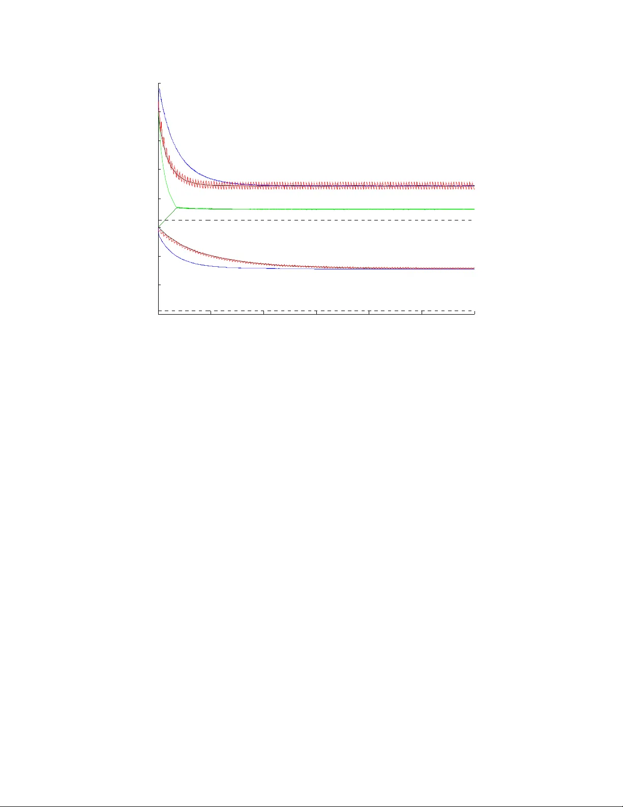
Sc heduling Kalman Filters in Con tin uous Time Jerome Le Ny , Eric F eron and Mun ther Dahleh ∗ Octob er 29, 2018 Abstract A set of N indep enden t Gaussian linear time in v ariant systems is observ ed by M sensors whose task is to provide the best p ossible steady-state causal minimum mean square estimate of the state of the systems, in addition to minimizing a steady-state measuremen t cost. The sensors can switch betw een systems instan taneously , and there are additional resource constraints, for example on the n umber of sensors which can observ e a giv en system sim ultaneously . W e first derive a tractable relaxation of the problem, whic h pro vides a bound on the ac hiev able p erformance. This bound can b e computed by solving a con vex program in v olving linear matrix inequalities. Exploiting the additional structure of the sites ev olving indep endently , we can decomp ose this program in to coupled smaller dimensional problems. In the scalar case with iden tical sensors, w e giv e an analytical expression of an index p olicy prop osed in a more general con text by Whittle. In the general case, we dev elop op en-lo op p erio dic switching p olicies whose performance matc hes the b ound arbitrarily closely . 1 In tro duction Adv ances in sensor net w orks and the dev elopment of unmanned v ehicle systems for intel- ligence, reconnaissance and surv eillance missions require the developmen t of data fusion sc hemes that can handle measuremen ts originating from a large num b er of sensors observing a large n um b er of targets, see e.g. [ 1 , 2 ]. These problems hav e a long history [ 3 ], and can b e used to formulate static sensor scheduling problems as well as tra jectory optimization problems for mobile sensors [ 4 , 5 ]. ∗ J. Le Ny is with the Department of Electrical and Systems Engineering, Universit y of Pennsylv ania, Philadelphia, P A 19104, USA jeromel@seas.upenn.edu. M. Dahleh is with the Laboratory for Infor- mation and Decision Systems, Massach usetts Institute of T echnology , Cambridge, MA 02139-4307, USA dahleh@mit.edu. E. F eron is with the School of Aerospace Engineering, Georgia T ec h, Atlan ta, GA 30332, USA eric.feron@aerospace.gatech.edu. 1 In this pap er, we consider M mobile sensors trac king the state of N sites or targets in con tin uous time. W e assume that the sites can b e describ ed b y N plants with independent linear time inv ariant dynamics, ˙ x i = A i x i + B i u i + w i , x i (0) = x i, 0 , i = 1 , . . . , N . W e assume that the plan t controls u i ( t ) are deterministic and known for t ≥ 0. Eac h driving noise w i ( t ) is a stationary white Gaussian noise pro cess with zero mean and kno wn p o wer sp ectral density matrix W i : Co v( w i ( t ) , w i ( t 0 )) = W i δ ( t − t 0 ) . The initial conditions are random v ariables with known mean ¯ x i, 0 and co v ariance matrices Σ i, 0 . By indep enden t systems w e mean that the noise pro cesses of the different plan ts are indep enden t, as w ell as the initial conditions x i, 0 . Moreov er the initial conditions are assumed indep enden t of the noise processes. W e shall assume in addition that Assumption 1. The matric es Σ i, 0 ar e p ositive definite for al l i ∈ { 1 , . . . , N } . This can b e achiev ed b y adding an arbitrarily small m ultiple of the identit y matrix to a p oten tially non inv ertible matrix Σ i, 0 . This assumption is needed in our discussion to b e able to use the information filter later on and to use a tec hnical theorem on the con vergence of the solutions of a p erio dic Riccati equation in section 4.3.2 . W e assume that we hav e at our disp osal M sensors to observ e the N plan ts. If sensor j is used to observe plant i , w e obtain measuremen ts y ij = C ij x i + v ij . Here v ij is a stationary white Gaussian noise pro cess with p o wer sp ectral density matrix V ij , assumed p ositiv e definite. Also, v ij is indep enden t of the other measuremen t noises, process noises, and initial states. Finally , to guaran tee conv ergence of the filters later on, w e assume throughout that Assumption 2. F or al l i ∈ { 1 , . . . , N } , ther e exists a set of indic es j 1 , j 2 , . . . , j n i ∈ { 1 , . . . , M } such that the p air ( A i , ˜ C i ) is dete ctable, wher e ˜ C i = [ C T ij 1 , . . . , C T ij n i ] T . Assumption 3. F or al l i ∈ { 1 , . . . , N } , the p air ( A i , W 1 / 2 i ) is c ontr ol lable. Let us define π ij ( t ) = ( 1 if plant i is observed at time t by sensor j 0 otherwise. W e assume that each sensor can observ e at most one system at eac h instan t, hence we ha ve the constrain t N X i =1 π ij ( t ) ≤ 1 , ∀ t, j = 1 , . . . , M . (1) 2 If instead sensor j is required to b e alw a ys op erated, constrain t ( 1 ) should simply b e c hanged to N X i =1 π ij ( t ) = 1 . (2) The equalit y constrain t is useful in scenarios in v olving sensors moun ted on unmanned v ehicles for example, where it might not b e p ossible to withdraw a v ehicle from op eration during the mission. The p erformance will b e w orse in general than with an inequalit y constraint once w e in tro duce op eration costs. W e also add the follo wing constraint, similar to the one used b y Athans [ 6 ]. W e supp ose that eac h system can b e observ ed b y at most one sensor at each instant, so w e ha ve M X j =1 π ij ( t ) ≤ 1 , ∀ t, i = 1 , . . . , N . (3) Similarly if system i must alw a ys b e observ ed by some sensor, constraint ( 3 ) can b e c hanged to an equality constraint M X j =1 π ij ( t ) = 1 . (4) Note that a sensor in our discussion can corresp ond to a com bination of several physical sensors, and so the constraints ab o ve can capture seemingly more general problems where w e allo w for example more that one simultaneous measuremen ts p er system. Using ( 4 ) we could also imp ose a constraint on the total num b er of allow ed observ ations at eac h time. Indeed, consider a constrain t of the form N X i =1 M X j =1 π ij ( t ) ≤ p, for some p ositive integer p. This constrain t means that M − p sensors are required to be idle at eac h time. So w e can create M − p “dumm y” systems (we should choose simple scalar stable systems to minimize computations), and asso ciate the constrain t ( 4 ) to each of them. Then w e simply do not include the cov ariance matrix of these systems in the ob jective function ( 5 ) below. W e consider an infinite-horizon av erage cost problem. The parameters of the mo del are assumed kno wn. W e wish to design an observ ation p olicy π ( t ) = { π ij ( t ) } satisfying the constrain ts ( 1 ), ( 3 ), or their equalit y versions, and an estimator ˆ x π of x , dep ending at e ach instant only on the p ast and curr ent observations pr o duc e d by the observation p olicy , such that the a v erage error co v ariance is minimized, in addition to some observ ation costs. The p olicy π itself can also only dep end on the past observ ations. More precisely , we wish to minimize, sub ject to the constraints ( 1 ), ( 3 ), J av g = min π , ˆ x π lim sup T →∞ 1 T E " Z T 0 N X i =1 ( x i − ˆ x π ,i ) 0 T i ( x i − ˆ x π ,i ) + M X j =1 κ ij π ij ( t ) ! dt # , (5) 3 where the constants κ ij are a cost paid p er unit of time when plant i is observ ed by sensor j . The T i ’s are p ositive semidefinite w eighting matrices. Liter atur e R eview and Contributions of this p ap er . The sensor scheduling problem presented ab o v e, except for minor v ariations, is an infinite horizon v ersion of the problem considered by A thans in [ 6 ]. See also Meier et al. [ 3 ] for the discrete-time v ersion. Athans considered the observ ation of only one plant. W e include here several plan ts to sho w how their indep endent ev olution prop ert y can b e leveraged in the computations, using the dual decomp osition metho d from optimization. Discrete-time versions of this sensor selection problem hav e received a significan t amoun t of atten tion, see e.g. [ 7 , 8 , 9 , 4 , 10 , 11 , 12 ]. All algorithms prop osed so far, except for the optimal greedy policy of [ 11 ] in the completely symmetric case, either run in exp onential time or consist of heuristics with no p erformance guaran tee. W e do not consider the discrete-time problem in this pap er. Finite-horizon contin uous-time v ersions of the problem, b esides the presen tation of Athans [ 6 ], ha ve also b een the sub ject of several pap ers [ 13 , 14 , 15 , 16 ]. The solutions prop osed, usually based on optimal con trol tec hniques, also in v olv e computational pro cedures that scale p oorly with the dimension of the problem. Somewhat surprisingly ho wev er, and with the exception of [ 17 ], it seems that the infinite- horizon con tin uous time version of the Kalman filter sc heduling problem has not been consid- ered previously . Mourikis and Roumeliotis [ 17 ] consider initially also a discrete time v ersion of the problem for a particular rob otic application. Ho w ever, their discrete mo del originates from the sampling at high rate of a contin uous time system. T o cop e with the difficult y of determining a sensor schedule, they assume instead a mo del where each sensor can in- dep enden tly pro cess eac h of the a v ailable measurements at a constan t frequency , and seek the optimal measuremen t frequencies. In fact, they obtain these frequencies by introducing heuristically a con tin uous time Riccati equation, and show that the frequencies can then b e computed by solving a semidefinite program. In contrast, we consider the more standard sc hedule-based v ersion of the problem in contin uous time, whic h is a priori more constrain- ing. W e show that essentially the same con v ex program pro vides in fact a lower b ound on the cost ac hiev able b y any measurement p olicy . In addition, we provide additional insight in to the decomp osition of the computations of this program, whic h can b e useful in the framew ork of [ 17 ] as w ell. The rest of the c hapter is organized as follo ws. Section 2 briefly recalls that for a fixed p olicy π ( t ), the optimal estimator is obtained by a type of Kalman-Bucy filter. The prop erties of the Kalman filter (indep endence of the error co v ariance matrix with resp ect to measuremen t v alues) imply that the remaining problem of finding the optimal scheduling p olicy π is a deterministic con trol problem. In section 3 w e treat a simplified scalar v ersion of the problem with identical sensors as a sp ecial case of the classical “Restless Bandit Problem” (RBP) [ 18 ], and provide analytical expressions for an index p olicy and for the elements necessary to compute efficien tly a low er b ound on p erformance, b oth of whic h w ere prop osed in the general setting of the RBP b y Whittle. Then, for the m ultidimensional case treated in full generalit y in section 4 , we sho w that the low er b ound on p erformance can be computed as a con vex program inv olving linear matrix inequalities. This low er b ound can b e approached 4 arbitrarily closely by a family of new p erio dically switching p olicies describ ed in section 4.3 . Approac hing the b ound with these p olicies is limited only b y the frequency with which the sensors can actually switc h b et w een the systems. In general, our solution has muc h more attractiv e computational properties than the solutions prop osed so far for the finite-horizon problem. 2 Optimal Estimator F or a given observ ation p olicy π ( t ) = { π ij ( t ) } i,j , the minimum v ariance filter is given b y the Kalman-Bucy filter [ 19 ], see [ 6 ]. The state estimates ˆ x π , where the subscript indicates the dep endency on the p olicy π , are all up dated in parallel following the sto chastic differen tial equation d dt ˆ x π ,i ( t ) = A i ˆ x π ,i ( t ) + B i ( t ) u i ( t ) + Σ π ,i ( t ) M X j =1 π ij ( t ) C T ij V − 1 ij ( C ij ˆ x π ,i ( t ) − y ij ( t )) ! , ˆ x π ,i (0) = ¯ x i, 0 . The resulting estimator is unbiased and the error co v ariance matrix Σ π ,i ( t ) for site i verifies the matrix Riccati differen tial equation d dt Σ π ,i ( t ) = A i Σ π ,i ( t ) + Σ π ,i ( t ) A T i + W i − Σ π ,i ( t ) M X j =1 π ij ( t ) C T ij V − 1 ij C ij ! Σ π ,i ( t ) , (6) Σ π ,i (0) = Σ i, 0 . With this result, we can reform ulate the optimization of the observ ation p olicy as a deter- ministic optimal con trol problem. Rewriting E (( x i − ˆ x i ) 0 T i ( x i − ˆ x i )) = T r ( T i Σ i ) , the problem is to compute min π lim sup T →∞ 1 T " Z T 0 N X i =1 T r ( T i Σ π ,i ( t )) + M X j =1 κ ij π ij ( t ) ! dt # , (7) sub ject to the constrain ts ( 1 ), ( 3 ), or their equality versions, and the dynamics ( 6 ). 3 Sites with One-Dimensional Dynamics and Iden tical Sensors W e assume in this section that 5 1. the sites or targets ha ve one-dimensional dynamics, i.e., x i ∈ R , i = 1 , . . . , N ; and, 2. all the sensors are iden tical, i.e., C ij = C i , V ij = V i , κ ij = κ i , j = 1 , . . . , M . Because of condition 2 , w e can simplify the problem form ulation intr o duced ab o v e so that it corresponds exactly to a sp ecial case of the Restless Bandit Problem [ 18 ]. W e define π i ( t ) = ( 1 if plant i is observed at time t by a sensor 0 otherwise. Since w e assumed that a system can b e observed by at most one sensor, the scheduling problem is interesting only in the case M < N . Note that a constraint ( 4 ) for some system i can b e eliminated, by remo ving one av ailable sensor, whic h is alw a ys measuring the system i . Constrain ts ( 2 ) and ( 3 ) can then b e replaced by the single constraint N X i =1 π i ( t ) = M , ∀ t. This constrain t means that at eac h perio d, exactly M of the N sites are observ ed. W e treat this case in this section, but again the equality sign can b e c hanged to an inequality with v ery little change in our discussion. T o obtain a low er b ound on the achiev able p erformance, w e relax the constraint to enforce it only on a v erage lim sup T →∞ 1 T Z T 0 N X i =1 π i ( t ) dt = M . (8) Then w e adjoin this constrain t using a (scalar) Lagrange m ultiplier λ to form the Lagrangian L ( π , λ ) = lim sup T →∞ 1 T Z T 0 N X i =1 [T r ( T i Σ π ,i ( t )) + ( κ i + λ ) π i ( t )] dt − λM . Here κ i is the cost p er time unit for observing site i . The dynamics of Σ π ,i are no w giv en by d dt Σ π ,i ( t ) = A i Σ π ,i ( t ) + Σ π ,i ( t ) A 0 i + W i − π i ( t ) Σ π ,i ( t ) C T i V − 1 i C i Σ π ,i ( t ) , (9) Σ π ,i (0) = Σ i, 0 . Then the original optimization problem ( 7 ) with the relaxed constrain t ( 8 ) can b e expressed as γ = inf π sup λ L ( π , λ ) = sup λ inf π L ( π , λ ) , where the exc hange of the suprem um and the infimum can be justified using a minimax theo- rem for constrained dynamic programming [ 20 ]. W e are then led to consider the computation of the dual function γ ( λ ) = min π lim sup T →∞ 1 T Z T 0 N X i =1 [T r ( T i Σ π ,i ( t )) + ( κ i + λ ) π i ( t )] dt − λM , 6 whic h has the imp ortant prop ert y of b eing sep ar able by site , i.e., γ ( λ ) + λM = P N i =1 γ i ( λ ), where for each site i we hav e γ i ( λ ) = min π i lim sup T →∞ 1 T Z T 0 T r ( T i Σ π i ,i ( t )) + ( κ i + λ ) π i ( t ) dt. (10) When the dynamics of the sites are one dimensional, i.e., Σ i ∈ R , w e can solv e this optimal con trol problem for each site analytically , that is, we obtain an analytical expression of the dual function, whic h pro vides a low er b ound on the cost for each λ . The computations are presen ted in paragraph ( 3.2 ). First, we explain ho w these computations will also pro vide the elemen ts necessary to design a scheduling p olicy . 3.1 Restless Bandits The Restless Bandit Problem (RBP) w as introduced by Whittle in [ 18 ] as a generalization of the classical Multi-Armed Bandit Problem (MABP), which w as first solved by Gittins [ 21 ]. In the RBP , w e ha ve N pro jects ev olving independently , M of whic h can be activ ated at eac h time. Pro jects that are activ e can ev olv e according to differen t dynamics than pro ject that remain passiv e. In our problem, the pro jects corresp ond to the systems and their activ ation corresp onds to taking a measuremen t. W e describ e in our particular con text the index p olicy prop osed b y Whittle for the RBP , whic h, although sub optimal in general, generalizes the optimal policy of Gittins’ in the case of the MABP . Consider the ob jective ( 10 ) for system i . Clearly , the Lagrange multiplier λ can b e in terpreted as a tax p enalizing measuremen ts of the system. As λ increases, the passive action (i.e., not measuring) should b ecome more attractiv e. F or a given v alue of λ , let us denote P i ( λ ) the set of co v ariance matrices Σ i for whic h the passiv e action is optimal. Let S n + b e the set of symmetric positive semidefinite matrices. Then we say that Definition 4. System i is indexable if and only if P i ( λ ) is monotonic al ly incr e asing (in the sense of set inclusion) fr om ∅ to S n + as λ incr e ases fr om −∞ to + ∞ . If system i is indexable, we define its Whittle index by λ i (Σ i ) = inf { λ ∈ R : Σ i ∈ P i ( λ ) } . Ho w ever natural the indexabilit y requirement might app ear, Whittle provided an example of an RBP where it is not v erified. W e will see in the next paragraph how ever that for our particular problem, at least in the scalar case, indexabilit y of the systems is guaran teed. The idea b ehind the definition of the Whittle index consists in defining an in trisic “v alue” for the measurement of system i , taking into account b oth the immediate and future gains. If the cov ariance of system i is Σ i , the Whittle index defines this v alue as the measurement tax (p otentially negativ e) that should b e required to mak e the con troller indifferen t b et w een measuring and not measuring the system. Finally , if all the systems are indexable, the Whittle p olicy cho oses at e ach instant to me asur e the M systems with highest Whittle index . There is significant exp erimen tal data and some theoretical evidence indicating that when the Whittle p olicy is well-defined for an RBP , its p erformance is often very close to optimal, see e.g. [ 22 , 23 , 24 ]. 7 3.2 Solution of the Scalar Optimal Con trol Problem W e can no w consider problem ( 10 ) for a single site, dropping the index i . W e return to the scalar case Σ ∈ R . The dynamical ev olution of the v ariance ob eys the equation ˙ Σ = 2 A Σ + W − π C 2 V Σ 2 , with π ( t ) ∈ { 0 , 1 } . The Hamilton-Jacobi-Bellman (HJB) equation is γ ( λ ) = min  T Σ + (2 A Σ + W ) h 0 (Σ; λ ) , T Σ + κ + λ + (2 A Σ + W − C 2 V Σ 2 ) h 0 (Σ; λ )  , (11) where h is the relative v alue function. W e will use the follo wing notation. Consider the algebraic Riccati equation (ARE) 2 Ax + W − C 2 V x 2 = 0 . First, if T = 0, it is clearly optimal to alwa ys observe if λ + κ < 0 and alw ays observ e otherwise. Hence the Whittle index is λ (Σ) = − κ for all Σ ∈ R + , and γ ( λ ) = min { κ + λ, 0 } . So w e can now assume T > 0. If C = 0, the solution to ( 11 ) is to alw a ys observ e if ( κ + λ ) < 0 and nev er observ e otherwise. Hence the Whittle index is again λ (Σ) = − κ for all Σ ∈ R + and w e get, b y letting Σ = − W 2 A in the HJB equation for a stable system: for C=0: γ ( λ ) =      − T W 2 A + κ + λ if the system is stable ( A < 0) and ( κ + λ ) < 0 , − T W 2 A if the system is stable and ( κ + λ ) ≥ 0 , + ∞ otherwise ( A ≥ 0) . The third case is clear from the fact that the system is unstable and cannot b e measured. So w e can no w assume that C 6 = 0. Then the ARE has t wo ro ots x 1 = A − p A 2 + C 2 W /V C 2 /V , x 2 = A + p A 2 + C 2 W /V C 2 /V . By assumption 3 , W 6 = 0 and so x 1 is strictly negative and x 2 is strictly p ositive. W e can treat the case κ + λ < 0 immediately . Then it is ob viously optimal to alw a ys observ e, and w e get, letting Σ = x 2 in the HJB equation: γ ( λ ) = T x 2 + κ + λ. So from no w on w e can assume λ ≥ − κ . Let us temp orarily assume the follo wing result on the form of the optimal p olicy . The v alidity of this assumption can b e verified a p osteriori from the form ulas obtained b elow, using the fact that the dynamic programming equation pro vides a sufficient condition for optimalit y of a solution. F orm of the optimal p olicy . The optimal p olicy is a threshold p olicy , i.e., it observ es the system for Σ ≥ Σ th and does not observ e for Σ < Σ th , for some Σ th ∈ R + . 8 W e would like to obtain the v alue of the av erage cost γ ( λ ) and of the threshold Σ th ( λ ). Note that w e already kno w Σ th ( λ ) = 0 for λ ≤ − κ , and we ha ve P ( λ ) = [0 , Σ th ( λ )] for the passiv e region P ( λ ) of definition 4 . Then the system is indexable if and only if Σ th ( λ ) is an increasing function of λ , and then inv erting the relation λ 7→ Σ th ( λ ) giv es the Whittle index Σ 7→ λ (Σ). 3.2.1 Case Σ th ≤ x 2 In this case, w e obtain as b efore γ ( λ ) = T x 2 + κ + λ. (12) This is intuitiv ely clear for Σ th < x 2 : ev en when observing the system all the time, the v ariance still conv erges in finite time to a neigh b orho o d of x 2 . Since this neigh b orho o d is in the active region by h yp othesis, after p oten tially a transition perio d (if the v ariance started at a v alue smaller than Σ th ), we should alwa ys observ e, and so the infinite-horizon a verage cost is the same as for the policy that alw a ys observ es. By con tinuit y at the interface b et ween the activ e and passive regions, w e ha ve T Σ th + (2 A Σ th + W ) h 0 (Σ th ) = T Σ th + ( κ + λ ) + (2 A Σ th + W − C 2 V Σ 2 th ) h 0 (Σ th ) i.e., κ + λ = C 2 V Σ 2 th h 0 (Σ th ) . W e ha ve then C 2 V Σ 2 th ( T x 2 + κ + λ ) = C 2 V T Σ 3 th + (2 A Σ th + W )( κ + λ )  − C 2 V Σ 2 th + 2 A Σ th + W  ( κ + λ ) = C 2 V Σ 2 th T ( x 2 − Σ th ) − (Σ th − x 2 )(Σ th − x 1 )( κ + λ ) = Σ 2 th T ( x 2 − Σ th ) (since C 6 = 0) T Σ 2 th − Σ th ( κ + λ ) + x 1 ( κ + λ ) = 0 so λ (Σ th ) = − κ + T Σ 2 th Σ th − x 1 , Σ th ( λ ) = κ + λ T + q ( κ + λ T )( κ + λ T − 4 x 1 ) 2 . (13) Expressions ( 12 ) and ( 13 ) are v alid under the condition Σ th ( λ ) ≤ x 2 . Note from ( 13 ) that Σ th 7→ λ (Σ th ) is an increasing function and the functions λ ( · ) and Σ th ( · ) are inv erse of eac h other. 3.2.2 Case Σ th > x 2 It turns out that in this case we must distinguish b etw een stable and unstable systems. F or a stable system ( A < 0), the Lyapuno v equation 2 Ax + W = 0 9 has a strictly p ositiv e solution x e = − W 2 A , with x e > x 2 since C 6 = 0. Stable System ( A < 0 ) with Σ th ≥ x e : In this case we know that x e is in the passive region. Hence, with Σ = x e in the HJB equation, w e get γ ( λ ) = T x e . (14) Then we ha v e again κ + λ = C 2 V Σ 2 th h 0 (Σ th ) , and no w T Σ th + (2 A Σ th + W ) h 0 (Σ th ) = T x e . Hence C 2 V Σ 2 th T ( x e − Σ th ) = (2 A Σ th + W )( κ + λ ) = 2 A (Σ th − x e )( κ + λ ) λ (Σ th ) = − κ + C 2 T Σ 2 th 2 | A | V , Σ th ( λ ) = q 2 | A | V λ + κ T | C | . (15) Stable System ( A < 0 ) with x 2 < Σ th < x e , or non-stable system ( A ≥ 0 ) : If the system is marginally stable or unstable, we cannot define x e . W e can think of this case as x e → ∞ as A → 0 − , and treat it sim ultaneously with the case where the system is stable and x 2 < Σ th < x e . Then x 2 is in the passive region, and x e is in the active region, so the prefactors of h 0 ( x ) in the HJB equation do not v anish. There is no immediate relation pro viding the v alue of γ ( λ ). W e can use the smo oth-fit principle to handle this case and obtain the expression of the Whittle indices, following [ 18 ]. Again the formal justification comes from using the final expressions of the v alue function thus obtained to v erify that it indeed satisfies the HJB equation. Theorem 1 ([ 18 ],[ 25 ]) . Consider a c ontinuous-time one-dimensional r estless b andit pr oje ct x ( t ) ∈ R satisfying ˙ x ( t ) = a k ( x ) , k = 0 , 1 , with p assive and active c ost r ates r k ( x ) , k = 0 , 1 . Assume that a 0 ( x ) do es not vanish in the optimal p assive r e gion, and a 1 ( x ) do es not vanish in the optimal active r e gion. Then the Whittle index is given by λ ( x ) = r 0 ( x ) − r 1 ( x ) + [ a 1 ( x ) − a 0 ( x )][ a 0 ( x ) r 0 1 ( x ) − a 1 ( x ) r 0 0 ( x )] a 0 ( x ) a 0 1 ( x ) − a 1 ( x ) a 0 0 ( x ) . Remark 5. The assumption that a 0 and a 1 do not vanish in the optimal p assive and active r e gions r esp e ctively excludes the c ases pr eviously studie d. It is missing fr om [ 18 ], [ 25 ], which ther efor e pr ovide only an inc omplete description of the Whittle indic es for one-dimensional c ontinuous-time deterministic pr oje cts. Pr o of. The deriv ation of the expression of the Whittle index can b e found in [ 18 ], [ 25 , p.53], and is v alid only under the additional assumption mentioned ab o ve. 10 Corollary 6. The Whittle index for the c ase x 2 < Σ th < x e is given by: λ (Σ th ) = − κ + C 2 2 V T Σ 3 th A Σ th + W . (16) Pr o of. F or x 2 < Σ th < x e , the assumptions of theorem 1 are v erified with a 0 (Σ) = 2 A Σ + W, a 1 (Σ) = 2 A Σ + W − C 2 V Σ 2 r 0 (Σ) = T Σ , r 1 (Σ) = T Σ + κ. The result follo ws by a straightforw ard calculation. Note the expression for λ (Σ) indeed mak es sense since w e can verify that it defines an increasing function of Σ. With the v alue of the Whittle index, w e can finish the computation of the lo wer b ound γ ( λ ) for the case x 2 < Σ th < x e . Inv erting the relation ( 16 ), we obtain, for a given v alue of λ , the b oundary Σ th ( λ ) b et w een the passive and active regions. Σ th ( λ ) v erifies the depressed cubic equation X 3 − 2 V ( λ + κ ) T C 2 A X − 2 V ( λ + κ ) T C 2 W = 0 . (17) F or λ + κ ≥ 0, by Descartes’ rule of signs, this p olynomial has exactly one p ositive ro ot, whic h is Σ th ( λ ). The HJB equation then reduces to γ ( λ ) = T Σ + h 0 (Σ)(2 A Σ + W ) , for Σ < Σ th ( λ ) (18) γ ( λ ) = T Σ + κ + λ + h 0 (Σ)(2 A Σ + W − C 2 V Σ 2 ) , for Σ ≥ Σ th ( λ ) . (19) No w for x 2 < Σ th ( λ ) < x e , letting x = Σ th ( λ ) > 0 in the HJB equation, assuming con tin uit y of h 0 at the b oundary of the passive and activ e regions and eliminating h 0 (Σ th ( λ )), w e get γ ( λ ) = T Σ th ( λ ) + κ + λ + ( γ − T Σ th ( λ ))  1 − C 2 V (Σ th ( λ )) 2 2 A Σ th ( λ ) + W  ( γ ( λ ) − T Σ th ( λ ))  C 2 V (Σ th ( λ )) 2 2 A Σ th ( λ ) + W  = κ + λ γ ( λ ) = T Σ th ( λ ) + V ( κ + λ )(2 A Σ th ( λ ) + W ) C 2 (Σ th ( λ )) 2 , for x 2 < Σ th ( λ ) < x e . 3.2.3 Summary W e collect the previous computations in the follo wing theorem. 11 Theorem 2. In the one-dimensional Kalman filter sche duling pr oblem with identic al sensors, the systems ar e indexable. F or system i , the Whittle index λ i (Σ i ) is given as fol lows: • Case C = 0 or T = 0 : λ i (Σ i ) = − κ i , for al l Σ i ∈ R + . • Case C 6 = 0 and T 6 = 0 : λ i (Σ i ) =        − κ i + T i Σ 2 i Σ i − x 1 ,i if Σ i ≤ x 2 ,i , − κ i + C 2 i 2 V i T i Σ 3 i A i Σ i + W i if x 2 ,i < Σ i < x e,i , − κ i + T i C 2 i Σ 2 i 2 | A i | V i if x e,i ≤ Σ i , with the c onvention x e,i = + ∞ if A i ≥ 0 . The lower b ound on the achievable p erformanc e is obtaine d by maximizing the c onc ave function γ ( λ ) = N X i =1 γ i ( λ ) − λM (20) over λ , wher e the term γ i ( λ ) is given by • Case T = 0 : γ i ( λ ) = min { λ + κ i , 0 } . • Case T 6 = 0 , C = 0 : γ i ( λ ) = T i W i 2 | A i | + min { λ + κ i , 0 } if A i < 0 , γ i ( λ ) = + ∞ if A i ≥ 0 . • Case C 6 = 0 and T 6 = 0 : γ i ( λ ) =      T i x 2 ,i + κ i + λ if λ ≤ λ i ( x 2 ,i ) , T i Σ ∗ i ( λ ) + V i ( κ i + λ )(2 A i Σ ∗ i ( λ )+ W i ) C 2 i (Σ ∗ i ( λ )) 2 if λ i ( x 2 ,i ) < λ < λ i ( x e,i ) , T i x e,i if λ i ( x e,i ) ≤ λ. wher e in the se c ond c ase Σ ∗ i ( λ ) is the unique p ositive r o ot of ( 17 ). Pr o of. The indexability comes from the fact that the indices λ (Σ) are v erified to b e mono- tonically increasing functions of Σ. In verting the relation w e obtain Σ th ( λ ) as the v ariance for which w e are indifferen t b etw een the activ e and passive actions. As we increase λ , Σ th ( λ ) increases and the passiv e region (the in terv al [0 , Σ th ( λ )]) increases. 4 Multidimensional Systems Generalizing the computations of the previous section to m ultidimensional systems requires solving the corresponding optimal control problem in higher dimensions, for whic h it is not clear that a closed form solution exist. Moreov er we ha ve considered in section 3 a particular case of the sensor scheduling problem where all sensors are iden tical. W e now return to 12 the general multidimensional problem and sensors with p ossibly distinct characteristics, as describ ed in the in tro duction. F or the infinite-horizon a v erage cost problem, w e sho w that computing the v alue of a lo w er b ound similar to the one presen ted in section 3 reduces to a conv ex optimization problem in v olving, at worst, Linear Matrix Inequalities (LMI) whose size grows p olynomially with the problem essen tial parameters. Moreov er, one can further decomp ose the computation of this con vex program in to N coupled subproblems as in the standard restless bandit case. 4.1 P erformance Bound F or con venience, let us repeat the deterministic optimal con trol problem under consideration: min π lim sup T →∞ 1 T Z T 0 N X i =1 ( T r ( T i Σ i ( t )) + M X j =1 κ ij π ij ( t ) ) dt, (21) s.t. ˙ Σ i ( t ) = A i Σ i + Σ i A T i + W i − Σ i M X j =1 π ij ( t ) C T ij V − 1 ij C ij ! Σ i , i = 1 . . . , N , (22) π ij ( t ) ∈ { 0 , 1 } , ∀ t ≥ 0 , i = 1 . . . , N , j = 1 , . . . , M , N X i =1 π ij ( t ) ≤ 1 , ∀ t ≥ 0 , j = 1 , . . . , M , (23) M X j =1 π ij ( t ) ≤ 1 , ∀ t ≥ 0 , i = 1 , . . . , N , (24) Σ i (0) = Σ i, 0 , i = 1 , . . . , N . Here we consider the constraints ( 1 ) and ( 3 ), but any com bination of inequality and equality constrain ts from ( 1 )-( 4 ) can b e used without c hange in the argumen t for the deriv ation of the performance b ound. W e define the following quantities: ˜ π ij ( T ) = 1 T Z T 0 π ij ( t ) dt, ∀ T ≥ 0 . (25) Since π ij ( t ) ∈ { 0 , 1 } we must hav e 0 ≤ ˜ π ij ( T ) ≤ 1. Our first goal, inspired by the idea already exploited in the restless bandit problem, is to obtain a lo wer b ound on the cost of the finite-horizon optimal con trol problem in terms of the n umbers ˜ π ij ( T ) instead of the functions π ij ( t ). It will b e easier to work with the information matrices Q i ( t ) = Σ − 1 i ( t ) . Note that inv ertibility of Σ i ( t ) is guaranteed b y our assumptions, as a consequence of [ 26 , 13 theorem 21.1]. Hence w e replace the dynamics ( 22 ) by the equiv alen t ˙ Q i = − Q i A i − A T i Q i − Q i W i Q i + M X j =1 π ij ( t ) C T ij V − 1 ij C ij , i = 1 , . . . , N . (26) Let us also define, for all T , ˜ Σ i ( T ) := 1 T Z T 0 Σ i ( t ) dt, ˜ Q i ( T ) := 1 T Z T 0 Q i ( t ) dt. By linearit y of the trace op erator, w e can rewrite the ob jectiv e function lim sup T →∞ N X i =1 ( T r ( T i ˜ Σ i ( T )) + M X j =1 κ ij ˜ π ij ( T ) ) . Let S n , S n + , S n ++ denote the set of symmetric, symmetric p ositive semidefinite and symmetric p ositiv e definite matrices resp ectiv ely . A function f : R m → S n is called matrix c onvex if and only if for all x, y ∈ R m and α ∈ [0 , 1], w e ha v e f ( αx + (1 − α ) y )  αf ( x ) + (1 − α ) f ( y ) , where  refers to the usual partial order on S n , i.e., A  B if and only if B − A ∈ S n + . Equiv alen tly , f is matrix con v ex if the scalar function x 7→ z T f ( x ) z is con vex for all v ectors z . The follo wing lemma will b e useful Lemma 7. The functions S n ++ → S n ++ S n → S n X 7→ X − 1 X 7→ X W X for W ∈ S n + , ar e matrix c onvex. Pr o of. See [ 27 , p.76, p.110]. A consequence of this lemma is that Jensen’s inequalit y is v alid for these functions. W e use it first as follo ws ∀ T ,  1 T Z T 0 Σ i ( t ) dt  − 1  1 T Z T 0 Q i ( t ) dt = ˜ Q i ( T ) , hence ∀ T , ˜ Σ i ( T )  ( ˜ Q i ( T )) − 1 . and so T r ( T i ˜ Σ i ( T )) ≥ T r ( T i ( ˜ Q i ( T )) − 1 ) . 14 Next, in tegrating ( 26 ) and letting Q i, 0 = Σ − 1 i, 0 , w e ha ve 1 T ( Q i ( T ) − Q i, 0 ) = − ˜ Q i ( T ) A i − A T i ˜ Q i ( T ) − 1 T Z T 0 Q i ( t ) W i Q i ( t ) dt + M X j =1  1 T Z T 0 π ij ( t )  C T ij V − 1 ij C ij 1 T ( Q i ( T ) − Q i, 0 ) = − ˜ Q i ( T ) A i − A T i ˜ Q i ( T ) − 1 T Z T 0 Q i ( t ) W i Q i ( t ) dt + M X j =1 ˜ π ij ( T ) C T ij V − 1 ij C ij . Using Jensen’s inequality and lemma 7 again, w e ha ve 1 T Z T 0 Q i ( t ) W i Q i ( t )  ˜ Q i ( T ) W i ˜ Q i ( T ) , and so we obtain 1 T ( Q i ( T ) − Q i, 0 )  − ˜ Q i ( T ) A i − A T i ˜ Q i ( T ) − ˜ Q i ( T ) W i ˜ Q i ( T ) + M X j =1 ˜ π ij ( T ) C T ij V − 1 ij C ij . (27) Last, since Q i ( T )  0, this implies, for all T , ˜ Q i ( T ) A i + A T i ˜ Q i ( T ) + ˜ Q i ( T ) W i ˜ Q i ( T ) − M X j =1 ˜ π ij ( T ) C T ij V − 1 ij C ij  Q i, 0 T . (28) So w e see that for a fixed p olicy π and any time T , the quan tit y N X i =1 ( T r ( T i ˜ Σ i ( T )) + M X j =1 κ ij ˜ π ij ( T ) ) (29) is lo wer b ounded b y the quan tit y N X i =1 ( T r ( T i ( ˜ Q i ( T )) − 1 ) + M X j =1 κ ij ˜ π ij ( T ) ) , where the matrices ˜ Q i ( T ) and the n um b er ˜ π ij ( T ) are sub ject to the constrain ts ( 28 ) as well as 0 ≤ ˜ π ij ( T ) ≤ 1 , N X i =1 ˜ π ij ( T ) ≤ 1 , j = 1 , . . . , M , M X j =1 ˜ π ij ( T ) ≤ 1 , i = 1 , . . . , N . Hence for an y T , the quan tit y Z ∗ ( T ) defined b elow is a low er b ound on the v alue of ( 29 ) for 15 an y c hoice of p olicy π Z ∗ ( T ) = min ˜ Q i ,p ij N X i =1 ( T r ( T i ˜ Q − 1 i ) + M X j =1 κ ij p ij ) , (30) s.t. ˜ Q i A i + A T i ˜ Q i + ˜ Q i W i ˜ Q i − M X j =1 p ij C T ij V − 1 ij C ij  Q i, 0 T , i = 1 . . . , N , (31) ˜ Q i  0 , i = 1 . . . , N , 0 ≤ p ij ≤ 1 , i = 1 . . . , N , j = 1 , . . . , M , N X i =1 p ij ≤ 1 , j = 1 , . . . , M , M X j =1 p ij ≤ 1 , i = 1 , . . . , N . Consider now the following program, where the right-hand side of ( 31 ) has b een replaced b y 0: Z ∗ = min ˜ Q i ,p ij N X i =1 ( T r ( T i ˜ Q − 1 i ) + M X j =1 κ ij p ij ) , (32) s.t. ˜ Q i A i + A T i ˜ Q i + ˜ Q i W i ˜ Q i − M X j =1 p ij C T ij V − 1 ij C ij  0 , i = 1 . . . , N , (33) ˜ Q i  0 , i = 1 . . . , N , 0 ≤ p ij ≤ 1 , i = 1 . . . , N , j = 1 , . . . , M , N X i =1 p ij ≤ 1 , j = 1 , . . . , M , M X j =1 p ij ≤ 1 , i = 1 , . . . , N . Defining δ := 1 /T , and rewriting with a sligh t abuse of notation Z ∗ ( δ ) instead of Z ∗ ( T ) for δ p ositiv e, we also define Z ∗ (0) = Z ∗ , where Z ∗ is given b y ( 32 ). Note that Z ∗ (0) is finite, since w e can find a feasible solution as follo ws. F or eac h i , w e choose a set of indices J i = { j 1 , . . . , j n i } ⊂ { 1 , . . . , M } such that ( A i , ˜ C i ) is observ able, as in assumption 2 . Once a set J i has b een c hosen for each i , w e form the matrix ˆ P with elemen ts ˆ p ij = 1 { j ∈ J i } . Finally , w e form a matrix P with elemen ts p ij satisfying the constrain ts and nonzero exactly where the ˆ p ij are nonzero. Suc h a matrix is easy to find if w e consider the inequalit y constrain ts ( 1 ) and ( 3 ). If equality constrain ts are inv olved instead, suc h a matrix P exists as a consequence of Birkhoff theorem [ 28 ], see theorem 8 . Now w e consider the quadratic inequalit y ( 33 ) for some v alue of i . F rom the detectability assumption 2 and the c hoice of p ij , we deduce that 16 the pair ( A i , ˆ C i ), with ˆ C i = h √ p i 1 C T i 1 V − 1 / 2 i 1 · · · √ p iM C T iM V − 1 / 2 iM i T (34) is detectable. Also note that ˆ C T i ˆ C i = M X j =1 p ij C T ij V − 1 ij C ij . T ogether with the controllabilit y assumption 3 , w e then kno w that ( 33 ) has a p ositiv e definite solution ˜ Q i [ 29 , theorem 2.4.25]. Hence Z ∗ (0) is finite. W e can also define Z ∗ ( δ ) for δ < 0, b y changing the right-hand side of ( 31 ) into δ Q i, 0 = −| δ | Q i, 0 . W e hav e that Z ∗ ( δ ) is finite for δ < 0 small enough. Indeed, passing the term δ Q i, 0 on the left hand side, this can then b e seen as a p erturbation of the matrix ˆ C i ab o v e, and for δ small enough, detectability , which is an op en condition, is preserved. No w w e will see b elo w that ( 30 ), ( 32 ) are conv ex programs. It is then a standard result of p erturbation analysis (see e.g. [ 27 , p. 250]) that Z ∗ ( δ ) is a conv ex function of δ , hence con tin uous on the in terior of its domain, in particular con tinuous at δ = 0. So lim sup T →∞ Z ∗ ( T ) = lim T →∞ Z ∗ ( T ) = Z ∗ . Finally , for an y p olicy π , we obtain the follo wing low er b ound on the ac hiev able cost lim sup T →∞ 1 T Z T 0 N X i =1 ( T r ( T i Σ i ( t )) + M X j =1 κ ij π ij ( t ) ) dt ≥ lim T →∞ Z ∗ ( T ) = Z ∗ . W e now show how to compute Z ∗ b y solving a conv ex program in v olving linear matrix inequalities. F or eac h i , introduce a new (slac k) matrix v ariable R i . Since Q i  0 , R i  Q − 1 i is equiv alent, by taking the Sch ur complemen t, to  R i I I Q i   0 , and the Riccati inequalit y ( 33 ) can b e rewritten " ˜ Q i A i + A T i ˜ Q i − P M j =1 p ij C T ij V − 1 ij C ij ˜ Q i W 1 / 2 i W 1 / 2 i ˜ Q i − I #  0 . 17 W e finally obtain, dropping the tildes from the notation ˜ Q i , the semidefinite program Z ∗ = min R i ,Q i ,p ij N X i =1 ( T r ( T i R i ) + M X j =1 κ ij p ij ) , (35) s.t.  R i I I Q i   0 , i = 1 . . . , N , " Q i A i + A T i Q i − P M j =1 p ij C T ij V − 1 ij C ij Q i W 1 / 2 i W i Q 1 / 2 i − I #  0 , i = 1 . . . , N , 0 ≤ p ij ≤ 1 , i = 1 . . . , N , j = 1 , . . . , M , N X i =1 p ij ≤ 1 , j = 1 , . . . , M , (36) M X j =1 p ij ≤ 1 , i = 1 , . . . , N . Hence solving the program ( 35 ) provides a lo w er bound on the ac hiev able cost for the original optimal con trol problem. 4.2 Problem Decomp osition It is well-kno w that efficient metho ds exist to solve ( 35 ) in p olynomial time, which implies a computation time p olynomial in the n umber of v ariables of the original problem. Still, as the n um b er of targets increases, the large LMI ( 35 ) becomes difficult to solv e. Note ho wev er that it can b e decomposed in to N small coupled LMIs, follo wing the standard dual decomp osition approac h already used for the restless bandit problem. This decomp osition is very useful to solv e large scale programs with a large n um b er of systems. F or completeness, we presen t the argumen t in more details below. W e first note that ( 36 ) is the only constraint which links the N subproblems together. So w e form the Lagrangian L ( R, Q, p ; λ ) = N X i =1 ( T r ( T i R i ) + M X j =1 ( κ ij + λ j ) p ij ) − M X j =1 λ j , where λ ∈ R M + is a vector of Lagrange multipliers. W e would tak e λ ∈ R M if we had the constrain t ( 2 ) instead of ( 1 ). Now the dual function is G ( λ ) = N X i =1 G i ( λ ) − M X j =1 λ j , (37) 18 with G i ( λ ) = min R i ,Q i , { p ij } 1 ≤ j ≤ M T r ( T i R i ) + M X j =1 ( κ ij + λ j ) p ij , (38) s.t.  R i I I Q i   0 , " Q i A i + A T i Q i − P M j =1 p ij C T ij V − 1 ij C ij Q i W 1 / 2 i W 1 / 2 i Q i − I #  0 , 0 ≤ p ij ≤ 1 , j = 1 , . . . , M , M X j =1 p ij ≤ 1 . The optimization algorithm pro ceeds then as follows [ 30 , c hap. 11]. W e c ho ose an initial v alue λ 1 ≥ 0 and set k = 1. 1. F or i = 1 , . . . , N , compute R k i , Q k i , { p k ij } 1 ≤ j ≤ M optimal solution of ( 38 ), and the v alue G i ( λ k ). 2. The v alue of the dual function at λ k is giv en by ( 37 ). A sup ergradien t of G ( λ k ) at λ k is giv en b y " N X i =1 p k i 1 − 1 , . . . , N X i =1 p k iM − 1 # . 3. Compute λ k +1 in order to maximize G ( λ ). W e can do this by using a sup ergradien t algorithm, or any preferred nonsmo oth optimization algorithm. Let k:=k+1 and go to step 1 , or stop if conv ergence is satisfying. Because the initial program ( 35 ) is conv ex, w e know that the optimal v alue of the dual optimization problem is equal to the optimal v alue of the primal. Moreov er, the optimal v ariables of the primal are obtained at step 1 of the algorithm abov e once conv ergence has b een reached. 4.3 Op en-lo op P erio dic P olicies Ac hieving the P erformance Bound 4.3.1 Definition of the P olicies In this section w e describ e a sequence of op en-lo op p olicies that can approach arbitrarily closely the low er b ound computed by ( 35 ), thus pro ving that this b ound is tigh t. These p oli- cies are p erio dic switching strategies using a schedule obtained from the optimal parameters p ij . Assuming no switc hing times or costs, their p erformance approaches the b ound as the length of the switc hing cycle decreases to ward 0. 19 Let P = [ p ij ] 1 ≤ i ≤ N , 1 ≤ j ≤ M b e the matrix of optimal parameters obtained in the solution of ( 35 ). W e assume here that constrain ts ( 1 ) and ( 3 ) w ere enforced, which is the most general case for the discussion in this section. Hence P verifies 0 ≤ p ij ≤ 1 , i = 1 , . . . , N , j = 1 , . . . , M , N X i =1 p ij ≤ 1 , j = 1 , . . . , M , and M X j =1 p ij ≤ 1 , i = 1 , . . . , N . A doubly substo chastic matrix of dimension n is an n × n matrix A = [ a ij ] 1 ≤ i,j ≤ n whic h satisfies 0 ≤ a ij ≤ 1 , i, j = 1 , . . . , n, n X i =1 a ij ≤ 1 , j = 1 , . . . , n, and n X j =1 a ij ≤ 1 , i = 1 , . . . , n. If M = N , P is therefore a doubly substo c hastic matrix. Else if M < N (resp. N < M ) w e can add N − M columns of zeros (resp. M − N ro ws of zeros) to P to obtain a doubly substo c hastic matrix. In any case, w e call the resulting doubly substo c hastic matrix ˜ P = [ ˜ p ij ]. If ro ws ha v e b een added, this is equiv alent to the initial problem with additional “dumm y systems”. If columns are added, these corresp ond to using “dummy sensors”. Dumm y systems (i.e., for i > N ) are not included in the ob jectiv e function (the corresp onding T i is 0), and a dummy sensor (i.e., for j > M ) is asso ciated formally to the measuremen t noise co v ariance matrix V − 1 ij = 0 for all i , in effect pro ducing no measurement. In the follo wing w e assume that ˜ P is an N × N doubly substo c hastic matrix, but the discussion in the M × M case is iden tical. Doubly substo chastic matrices ha ve b een in tensiv ely studied, and the material used in the following can be found in the b o ok of Marshall and Olkin [ 31 ]. In particular, we ha v e the follo wing corollary of a classical theorem of Birkhoff [ 28 ], which says that a doubly sto c hastic matrix is a con vex combination of p erm utation matrices. Theorem 8 ([ 32 ]) . The set of N × N doubly substo chastic matric es is the c onvex hul l of the set P 0 of N × N matric es which have a most one unit in e ach r ow and e ach c olumn, and al l other entries ar e zer o. Hence for the doubly substochastic matrix ˜ P , there exists a set of p ositiv e n um b ers φ k and matrices P k ∈ P 0 suc h that ˜ P = K X k =1 φ k P k , with K X k =1 φ k = 1 , for some integer K . (39) One wa y of computing this decomp osition is to first extend ˜ P to the 2 N × 2 N doubly sto c hastic matrix ˆ P =  ˜ P I − D r I − D c ˜ P T  , 20 where r 1 , . . . , r N and c 1 , . . . , c N are the row sums and column sums of ˜ P , and D r = diag( r 1 , . . . , r N ), D c = diag( c 1 , . . . , c N ). Then there is an algorithm that runs in time O ( N 4 . 5 ) [ 31 , 33 ] and pro vides the decomp osition ˆ P = K X k =1 φ k ˆ P k , with K = (2 N − 1) 2 + 1 and where the ˆ P k ’s are p ermutation matrices of size 2 N × 2 N . The decomp osition ( 39 ) is finally obtained by deleting the last N ro ws and columns of ˆ P k to obtain the matrices P k , k = 1 , . . . , K . Note that any matrix A = [ a ij ] i,j ∈ P 0 represen ts a v alid sensor/system assignmen t (for the system with additional dumm y systems or sensors), where sensor j is measuring system i if and only if a ij = 1. With the decomp osition ( 39 ), w e now consider a family of p erio dic switc hing p olicies parametrized b y a p ositiv e num b er  represen ting a time interv al ov er whic h the switching schedule is executed completely . F or a given v alue of  , the p olicy is defined as follows: 1. A t time t = l , l ∈ N , asso ciate sensor j to system i as specified b y the matrix P 1 of the represen tation ( 39 ). Run the corresp onding contin uous-time Kalman filters, keeping this sensor/system asso ciation for a duration φ 1  . 2. A t time t = ( l + φ 1 )  , switch to the assignmen t sp ecified by P 2 . Run the corresp onding con tin uous time Kalman filters un til t = ( l + φ 1 + φ 2 )  . 3. Rep eat the switching pro cedure, switc hing to matrix P i +1 at time t = l + φ 1 + · · · + φ i , for i = 1 , . . . , K − 1. 4. A t time t = ( l + φ 1 + · · · + φ K )  = ( l + 1)  , start the switching sequence again at step 1 with P 1 and repeat the steps ab ov e. It is easy to see that the matrices P i , i = 1 , . . . , K nev er sp ecify that a “dumm y sensor” should execute a measuremen t or that a “dumm y system” should b e measured, since from the decomp osition ( 39 ) this would corresp ond to nonzero en tries in the columns or rows added to P to form ˜ P . 4.3.2 P erformance of the P erio dic Switc hing Policies Let us fix  > 0 in the definition of the switching p olicy , and consider no w, for this p olicy , the ev olution of the co v ariance matrix Σ  i ( t ) for the estimation error on the state of system i . The sup erscript indicates the dep endence on the p erio d  of the policy . First w e ha ve Lemma 9. F or al l i ∈ { 1 , . . . , N } , the estimation err or c ovarianc e Σ  i ( t ) c onver ges as t → ∞ to a p erio dic function ¯ Σ  i ( t ) of p erio d  . 21 Pr o of. Fix i ∈ { 1 , . . . , N } . Let σ i ( t ) ∈ { 0 , 1 , . . . , N } b e the function sp ecifying which sensor is observing system i at time t under the switc hing p olicy . By conv ention σ i ( t ) = 0 means that no sensor is sc heduled to observ e system i , and σ i ( t ) = j means that sensor j measures system i . Note from the remark following the description of the switc hing policies that in fact w e ha v e σ i ( t ) ∈ { 0 , . . . , M } , i.e., the p olicy nev er sc hedules measuremen ts by dummy sensors. Similarly , if instead we w ere considering the situation M > N and ˜ P an M × M matrix, then w e w ould ha v e σ i ( t ) = 0 for i ∈ { N + 1 , . . . , M } and all t . Note also that σ i ( t ) is a piecewise constan t,  -p erio dic function. The switching times of σ i ( t ) are t = ( l + φ 1 + · · · + φ k − 1 )  , for k = 1 , . . . , K and l ∈ N . The co v ariance matrix Σ  i ( t ) ob eys the follo wing perio dic Riccati differential equation (PRE): ˙ Σ  i ( t ) = A i Σ  i ( t ) + Σ  i ( t ) A T i + W i − Σ  i ( t )( C  i ( t )) T C  i ( t )Σ  i ( t ) (40) Σ  i ( t ) = Σ i, 0 , where C  i ( t ) := V − 1 / 2 iσ i ( t ) C iσ i ( t ) is a piecewise constant,  -perio dic matrix v alued function, and w e use the con v ention V − 1 ij = C ij = 0 when j = 0. W e now show that ( A i , C  i ( · )) is detectable. Let j 1 , . . . , j K b e the successiv e v alues taken b y the function σ i ( t ) ov er the p eriod  . F rom the definition of detectability for linear p erio dic systems and it modal c haracterization [ 34 , p.130], we immediately deduce that the pair ( A i , C  i ( · )) is not detectable if and only if there exists an eigenpair ( λ, x ) for A i , with Re( λ ) ≥ 0, x 6 = 0, suc h that A i x = λx, and C  i ( t ) e A i t x = e λt C  i ( t ) x = 0 , ∀ t ∈ [0 ,  ] , hence C ij 1 x = . . . = C ij K x = 0 . (41) Let us denote by p k,ij the ( i, j ) th elemen t of the matrix P k in the decomposition ( 39 ). W e ha ve p k,ij = 1 { j = j k } with the ab o ve definition of j k , including the case j k = 0 (no measurement), whic h giv es p k,ij = 0 for all j ∈ { 1 , . . . , N } . Then we can write K X k =1 φ k C T ij k V − 1 ij k C ij k = K X k =1 φ k N X j =1 p k,ij C T ij V − 1 ij C ij ! = N X j =1 K X k =1 φ k p k,ij ! C T ij V − 1 ij C ij = N X j =1 ˜ p ij C T ij V − 1 ij C ij = M X j =1 p ij C T ij V − 1 ij C ij = ˆ C T i ˆ C i , (42) where the next-to-last equalit y uses the fact that ˜ p ij = p ij for j ≤ M and ˜ p ij = 0 for j ≥ M + 1, and ˆ C i w as defined in ( 34 ). Note that w e now consider this definition of ˆ C i for the optimal parameters p ij pro vided by the solution of ( 35 ). Then ( 41 ) and ( 42 ) imply k ˆ C i x k 2 = 0, so ˆ C i x = 0, i.e., ( A, ˆ C i ) is not detectable. But the parameters p ij b eing 22 optimal for the program ( 35 ), this would imply that this program is not feasible [ 29 , p.68], a con tradiction with our discussion follo wing ( 34 ). So ( A i , C  i ( · )) m ust b e detectable, and together with our assumption 1 , this implies b y the result of [ 35 , p. 95] that lim t →∞  Σ  i ( t ) − ¯ Σ  i ( t )  = 0 , where ¯ Σ  i ( t ) is the strong solution of the PRE, which is  -p eriodic. Next, denote by ˜ Σ i ( t ) the solution to the following Riccati differen tial equation (RDE): ˙ Σ i = A i Σ i + Σ i A T i + W i − Σ i M X j =1 p ij C T ij V − 1 ij C ij ! Σ i , Σ i (0) = Σ i, 0 . (43) Assumptions 2 and 3 , together with our discussion of the implied detectability of the pair ( A, ˆ C i ) (see ( 42 )), guaran tee that ˜ Σ i ( t ) conv erges to a p ositiv e definite limit denoted Σ ∗ i . Moreo v er, Σ ∗ i is stabilizing and is the unique p ositive definite solution to the algebraic Riccati equation (ARE): A i Σ i + Σ i A T i + W i − Σ i M X j =1 p ij C T ij V − 1 ij C ij ! Σ i = 0 . (44) The next lemma sa ys that the p erio dic function ¯ Σ  i ( t ) oscillates in a neigh b orho o d of Σ ∗ i . Lemma 10. F or al l t ∈ R + , we have ¯ Σ  i ( t ) − Σ ∗ i = O (  ) as  → 0 . Pr o of. The function t → ¯ Σ  i ( t ) of lemma 9 is the strong p erio dic solution of the PRE ( 40 ). It is  -p erio dic. F rom Radon’s lemma [ 29 , p.90], whic h giv es a represen tation of the solution to a Riccati differential equation as the ratio of solutions to a linear ODE, we also know that ¯ Σ  i is C ∞ on eac h in terv al where σ i ( t ) is constan t, where σ i ( t ) is the switc hing signal defined in the pro of of lemma 9 . Let ˆ Σ  i b e the av erage of t → ¯ Σ  i ( t ): ˆ Σ  i = 1  Z  0 ¯ Σ  i ( t ) dt. F rom the preceding remarks, it is easy to deduce that for all t , we ha ve ¯ Σ  i ( t ) − ˆ Σ  i = O (  ) . No w, a veraging the PRE ( 40 ) ov er the in terv al [0 ,  ], w e obtain A i ˆ Σ  i + ˆ Σ  i A T + W i − 1  Z  0 ¯ Σ  i ( t )( C  i ( t )) T C  i ( t ) ¯ Σ  i ( t ) dt = 1  ( ¯ Σ  i (  ) − ¯ Σ  i (0)) = 0 , where C  i ( t ) was defined b elow displa y ( 40 ). Expanding this equation in p o wers of  , we get A i ˆ Σ  i + ˆ Σ  i A T + W i − ˆ Σ  i  1  Z  0 ( C  i ( t )) T C  i ( t ) dt  ˆ Σ  i + R (  ) = 0 , 23 where R (  ) = O (  ). Let j k := σ i ( t ) for t ∈ [( l + φ 1 + . . . + φ k − 1 ) , ( l + φ 1 + . . . + φ k )  ]. W e can then rewrite, using ( 42 ), 1  Z  0 ( C  i ( t )) T C  i ( t ) dt = K X k =1 φ k C T ij k V − 1 ij k C ij k = M X j =1 p ij C T ij V − 1 ij C ij . So w e obtain A i ˆ Σ  i + ˆ Σ  i A T + ( W i + R (  )) − ˆ Σ  i M X j =1 p ij C T ij V − 1 ij C ij ! ˆ Σ  i = 0 . Note moreo v er that for  sufficiently small, ˆ Σ  i is the unique p ositiv e definite stabilizing solution of this ARE, using the fact that con trolabilit y of ( A i , W 1 / 2 i ) is an op en condition. No w comparing this ARE to the ARE ( 44 ), and since the stabilizing solution of an ARE is a real analytic function of the parameters [ 36 ], we deduce that ˆ Σ  i − Σ ∗ i = O (  ), and the lemma. Theorem 11. L et Z  denote the p erformanc e of the p erio dic switching p olicy with p erio d  . Then Z  − Z ∗ = O (  ) as  → 0 , wher e Z ∗ is the p erformanc e b ound ( 35 ). Henc e the switching p olicy appr o aches the lower b ound arbitr arily closely as the p erio d tends to 0 . Pr o of. W e ha ve Z  = lim sup T →∞ 1 T Z T 0 N X i =1 T r ( T i Σ  i ( t )) + M X j =1 κ ij π  ij ( t ) ! dt, where π  is the sensor/system assignment of the switc hing p olicy . First by using a transfor- mation similar to ( 42 ) and using the con v en tion κ ij = 0 for j ∈ { 0 } ∪ { M + 1 , . . . , N } (no measuremen t or measurement by a dumm y sensor), we hav e for system i 1 T Z T 0 M X j =1 κ ij π ij ( t ) dt = 1 T b T  c− 1 X n =0 Z ( n +1)  n M X j =1 κ ij π ij ( t ) dt + 1 T Z T b T  c  M X j =1 κ ij π ij ( t ) dt = 1 T  T   K X k =1 κ ij k ( φ k  ) + 1 T Z T b T  c  M X j =1 κ ij π ij ( t ) dt =  T    T M X j =1 κ ij p ij + 1 T Z T b T  c  M X j =1 κ ij π ij ( t ) dt, (45) where the j k ’s w ere defined in the pro of of lemma 9 . Hence lim sup T →∞ 1 T Z T 0 N X i =1 M X j =1 κ ij π  ij ( t ) dt ≤ N X i =1 M X j =1 κ ij p ij . 24 Next, from lemma 9 and 10 , it follows readily that lim sup t →∞ Σ  i ( t ) − Σ ∗ i = O (  ). It is w ell kno wn [ 37 ] that under our assumptions Σ ∗ i is the minimal (for the partial order on S n + ) p ositiv e definite solution of the quadratic matrix inequalit y A i Σ i + Σ i A T i + W i − Σ i M X j =1 p ij C T ij V − 1 ij C ij ! Σ i  0 . Hence for the p ij obtained from the computation of the lo w er b ound ( 35 ), these matrices Σ ∗ i minimize N X i =1 T r ( T i Σ i ) s.t. A i Σ i + Σ i A T i + W i − Σ i M X j =1 p ij C T ij V − 1 ij C ij ! Σ i  0 , i = 1 , . . . , N . (46) Changing v ariable to Q i = Σ − 1 i , and multiplying the inequalities ( 46 ) on the left and righ t b y Q i yields Q i A i + A T i Q i + Q i W i Q i − M X j =1 p ij C T ij V − 1 ij C ij  0 , and hence we reco v er ( 33 ). In conclusion, the cov ariance matrices resulting from the switc hing p olicies approac h within O (  ) as  → 0 the cov ariance matrices which are obtained from the lo w er b ound on the ac hiev able cost. The theorem follo ws, b y upp er b ounding the supremum limit of a sum b y the sum of the suprem um limits to get Z ∗ ≤ Z  ≤ Z ∗ + O (  ). Remark 12. Sinc e the b ound c ompute d in ( 35 ) is tight, and sinc e it is e asy to se e that the p erformanc e b ound of se ction 3 is at le ast as go o d as the b ound ( 35 ) for the simplifie d pr oblem of that se ction, we c an c onclude that the two b ounds c oincide and that se ction 3 gives an alternative way of c omputing the solution of ( 35 ) in the c ase of identic al sensors and one-dimensional systems. Using the close d form expr ession for the dual function ( 20 ), we only ne e d to optimize over the unique L agr ange multiplier λ , indep endently of the numb er N of systems, inste ad of solving the LMI ( 35 ), for which the numb er of variables gr ows with N . 4.3.3 T ransien t Behavior of the Switc hing Policies Before we conclude, we tak e a lo ok at the transien t b eha vior of the switching p olicies. W e sho w that ov er a finite time interv al, Σ  i ( t ) remains close to ˜ Σ i ( t ), solution of the “av eraged” RDE ( 43 ). T ogether with the previous result of lemma 9 on the asymptotic b eha vior, we see then that Σ  i ( t ) and ˜ Σ i ( t ) remain close for all t . F or a matrix A , we denote b y k A k ∞ the maximal absolute v alue of the entries of A . Lemma 13. F or al l 0 ≤ T 0 < ∞ , ther e exist c onstants  0 > 0 and M 0 > 0 such that for al l 0 <  ≤  0 and for al l t ∈ [0 , T 0 ] , we have k Σ  i ( t ) − ˜ Σ i ( t ) k ∞ ≤ M 0  . 25 Pr o of. As in the pro of of lemma 10 , b y Radon’s lemma we know that Σ  i is C ∞ on eac h in terv al where σ i ( t ) is constan t. W e ha v e then, o v er the interv al t ∈ [ l, ( l + φ 1 )  ], for l ∈ N : Σ  i (( l + φ 1 )  ) = Σ  i ( l  ) + φ 1  [ A i Σ  i ( l  ) + Σ  i ( l  ) A T i + W i − Σ  i ( l  ) C T ij 1 V − 1 ij 1 C ij 1 Σ  i ( l  )] + O (  2 ) , (47) where as b efore we denote j k := σ i ( t ) for t ∈ [( l + φ 1 + . . . + φ k − 1 ) , ( l + φ 1 + . . . + φ k )  ]. Now o v er the p erio d t ∈ [( l + φ 1 ) , ( l + φ 1 + φ 2 )  ], w e ha ve: Σ  i (( l + φ 1 + φ 2 )  ) = Σ  i (( l + φ 1 )  ) + φ 2  [ A i Σ  i (( l + φ 1 )  ) + Σ  i (( l + φ 1 )  ) A T i + W i − Σ  i (( l + φ 1 )  ) C T ij 2 V − 1 ij 2 C ij 2 Σ  i (( l + φ 1 )  )] + O (  2 ) . Using ( 47 ), we deduce that Σ  i (( l + φ 1 + φ 2 )  ) =Σ  i ( l  ) +  [ φ 1 + φ 2 ] { A i Σ  i ( l  ) + Σ  i ( l  ) A T i + W i } −  Σ  i ( l  )( φ 1 C T ij 1 V − 1 ij 1 C ij 1 + φ 2 C T ij 2 V − 1 ij 2 C ij 2 )Σ  i ( l  ) + O (  2 ) . By immediate induction, and since φ 1 + · · · + φ K = 1, w e then hav e Σ  i (( l +1)  ) = Σ  i ( l  )+  ( A i Σ  i ( l  ) + Σ  i ( l  ) A T i + W i − Σ  i ( l  ) K X k =1 φ k C T ij k V − 1 ij k C ij k ! Σ  i ( l  ) ) + O (  2 ) . Hence b y ( 42 ), Σ  i v erifies the relation Σ  i (( l +1)  ) = Σ  i ( l  )+  ( A i Σ  i ( l  ) + Σ  i ( l  ) A T i + W i − Σ  i ( l  ) M X j =1 p ij C T ij V − 1 ij C ij ! Σ  i ( l  ) ) + O (  2 ) . (48) But notice now that the appro ximation ( 48 ) is also true b y definition for ˜ Σ i ( t ) o ver the in terv al t ∈ [ l , ( l + 1)  ]. Next, consider the following iden tit y for Q, X and ˜ X symmetric matrices: A ˜ X + ˜ X A T − ˜ X Q ˜ X − ( AX + X A T − X QX ) = ( A − ˜ X Q )( ˜ X − X ) + ( ˜ X − X )( A − ˜ X Q ) T + ( ˜ X − X ) Q ( ˜ X − X ) . Letting Q = P M j =1 p ij C T ij V − 1 ij C ij , ∆  i ( l ) = ˜ Σ i ( l  ) − Σ  i ( l  ), we obtain from this identit y ∆  i ( l + 1) = ∆  i ( l ) +  { ( A − ˜ Σ i ( l  ) Q )∆  i ( l ) + ∆  i ( l )( A − ˜ Σ i ( l  ) Q ) T + ∆  i ( l ) Q ∆  i ( l ) } + O (  2 ) . Note that ∆  i (0) = 0 and ˜ Σ i ( t ) is b ounded, so by immediate induction w e hav e ∆  i ( l ) = l X k =1 R k (  ) , where R k (  ) = O (  2 ) for all k . Fix T 0 ≥ 0. W e ha ve then ˜ Σ i  T 0     − Σ  i  T 0     = ∆  i  T 0   = O (  ) . This means that there exist constants  0 , M 0 > 0 suc h that     ˜ Σ i  T 0     − Σ  i  T 0         ∞ ≤ M 0 , for all 0 <  <  0 . It is easy to see from the argumen t ab o v e that a similar approximation is in fact v alid for all t up to time  T 0    . 26 0 1 2 3 4 5 6 1 2 3 4 5 6 7 8 9 Covariance Trajectories t Figure 1: Comparison of the v ariance tra jectories under Whittle’s index p olicy (solid blue curv es), the p erio dic switching p olicy (oscillating red curv es), and the greedy p olicy (con- v erging green curv es). The solid blac k curv es corresp ond to ˜ Σ i ( t ), solution of the RDE ( 43 ). Here a single sensor switches b et w een t w o scal ar systems. The p erio d  w as c hosen to b e 0 . 05. The system parameters are A 1 = 0 . 1 , A 2 = 2 , C i = Q i = R i = 1 , κ i = 0 for i = 1 , 2. The dashed lines are the steady-state v alues that could b e achiev ed with tw o iden tical sensors, eac h measuring one system. The p erformance of the Whittle p olicy is 7.98, whic h is optimal (i.e., matches the b ound). The p erformance of the greedy policy is 9 . 2. Note that the greedy p olicy mak es the v ariances conv erge, while Whittle’s p olicy makes the Whittle indices (not sho wn) conv erge. The switc hing p olicy sp ends 23% of its time measuring system 1 and 77% of its time measuring system 2. 4.3.4 Numerical Sim ulation Figure 1 compares the cov ariance tra jectories for Whittle’s index p olicy , the p erio dic switch- ing p olicy and the greedy p olicy (measuring the system with highest mean square error on the estimate) for a simple problem with one sensor switching b et w een tw o scalar systems. Significan t improv ements o ver the greedy p olicy can b e obtained in general b y using the p erio dic switc hing p olicies or the Whittle p olicy . An imp ortan t computational adv antage of the Whittle p olicy for large-scale problems with a limited num b er of iden tical sensors is that using the closed form solution of the indices pro vided in section 3.2.3 , it requires only ordering N num b ers (whic h is the same computational cost as for the greedy policy), whereas designing the op en-lo op switc hing p olicy requires computing a solution of the program ( 35 ). 27 5 Conclusion In this pap er, we hav e considered an atten tion-control problem in con tinuous time, whic h consists in scheduling sensor/target assignments and running the corresp onding Kalman filters. W e pro ved that the b ound obtained from a RBP type relaxation is tigh t, assuming w e allo w the sensors to switc h arbitrarily fast b et ween the targets. An op en question is to c haracterize the p erformance of the restless bandit index p olicy deriv ed in the scalar case. It was found experimentally that the p erformance of this p olicy seems to matc h the b ound, but we do not ha v e a pro of of this fact. An adv antage of the Whittle index p olicy ov er the switching p olicies is that it is in feedbac k form. Obtaining optimal feedback p olicies for the multidimensional case w ould also b e of in terest. F or practical applications, the main limitation of our mo del concerns the absence of switching costs and delays. Still, the optimal solution obtained in the absence of suc h costs should provide insight into the deriv ation of heuristics for more complex mo dels. Additionally there are numerous sensor sc heduling applications, suc h as for telemetry-data aerospace systems or radar w av eform selection systems, where the switc hing costs are not to o important. References [1] K. Chakrabart y , S. Sitherama Iy engar, H. Qi, and E. Cho, “Grid cov erage for surv eil- lance and target lo cation in distributed sensor net w orks,” IEEE T r ansactions on Com- puters , v ol. 51, no. 12, pp. 1448–1453, December 2002. [2] J. Cortes, S. Martinez, T. Karatas, and F. Bullo, “Co verage con trol for mobile sensing net w orks,” IEEE T r ansactions on R ob otics and A utomation , vol. 20, no. 2, pp. 243–255, April 2004. [3] L. Meier, J. Persc hon, and R. Dressler, “Optimal con trol of measurement systems,” IEEE T r ansactions on Automatic Contr ol , v ol. 12, no. 5, pp. 528–536, 1967. [4] A. Tiw ari, “Geometrical analysis of spatio-temp oral planning problems,” Ph.D. disser- tation, California Institute of T ec hnology , 2006. [5] J. Williams, “Information theoretic sensor managemen t,” Ph.D. dissertation, Mas- sac h usetts Institute of T ec hnology , F ebruary 2007. [6] M. A thans, “On the determination of optimal costly measurement strategies for linear sto c hastic systems,” Automatic a , v ol. 8, pp. 397–412, 1972. [7] E. F eron and C. Olivier, “T argets, sensors and infinite-horizon tracking optimalit y ,” in Pr o c e e dings of the 29th IEEE Confer enc e on De cision and Contr ol , 1990. [8] Y. Oshman, “Optimal sensor selection strategy for discrete-time state estimators,” IEEE T r ansactions on A er osp ac e and Ele ctr onic Systems , v ol. 30, no. 2, pp. 307–314, 1994. 28 [9] A. Tiw ari, M. Jun, D. E. Jeffcoat, and R. M. Murray , “Analysis of dynamic sensor co v erage problem using Kalman filters for estimation,” in Pr o c e e dings of the 16th IF A C World Congr ess , 2005. [10] V. Gupta, T. Ch ung, B. Hassibi, and R.M.Murray , “On a sto c hastic sensor selection algorithm with applications in sensor scheduling and sensor co v erage,” Automatic a , v ol. 42, no. 2, pp. 251–260, 2006. [11] B. F. L. Scala and B. Moran, “Optimal target tracking with restless bandits,” Digital Signal Pr o c essing , v ol. 16, pp. 479–487, 2006. [12] L. Shi, M. Epstein, B. Sinop oli, and R. Murra y , “Effective sensor sc heduling sc hemes in a sensor net work b y employing feedbac k in the communication lo op,” in Pr o c e e dings of the 16th IEEE International Confer enc e on Contr ol Applic ations , 2007. [13] E. Sk afidas and Nero de, “Optimal measurement sc heduling in linear quadratic gaussian con trol problems,” in Pr o c e e dings of the IEEE International Confer enc e on Contr ol Applic ations , T rieste, Italy , 1998, pp. 1225–1229. [14] A. Sa vkin, R. Ev ans, and E. Sk afidas, “The problem of optimal robust sensor sc hedul- ing,” Systems and Contr ol L etters , v ol. 43, pp. 149–157, 2001. [15] J. Baras and A. Bensoussan, “Optimal sensor sc heduling in nonlinear filtering of diffu- sion processes,” SIAM Journal on Contr ol and Optimization , vol. 27, no. 4, pp. 786–813, 1989. [16] H. Lee, K. T eo, and A. Lim, “Sensor schedu ling in contin uous time,” Automatic a , v ol. 37, pp. 2017–2023, 2001. [17] A. I. Mourikis and S. I. Roumeliotis, “Optimal sensor sc heduling for resource- constrained lo calization of mobile rob ot formations,” IEEE T r ansactions on R ob otics , v ol. 22, no. 5, pp. 917–931, 2006. [18] P . Whittle, “Restless bandits: activit y allo cation in a c hanging world,” Journal of Applie d Pr ob ability , v ol. 25A, pp. 287–298, 1988. [19] R. E. Kalman and R. S. Bucy , “New results in linear filtering and prediction,” Journal of Basic Engine ering (ASME) , v ol. 83D, pp. 95–108, 1961. [20] E. Altman, Constr aine d Markov De cision Pr o c esses . Chapman and Hall, 1999. [21] J. Gittins and D. Jones, “A dynamic allo cation index for the sequen tial design of ex- p erimen ts,” in Pr o gr ess in Statistics , J. Gani, Ed. Amsterdam: North-Holland, 1974, pp. 241–266. [22] K. Glazebro ok, D. Ruiz-Hernandez, and C. Kirkbride, “Some indexable families of rest- less bandit problems,” A dvanc es in Applie d Pr ob ability , v ol. 38, pp. 643–672, 2006. 29 [23] R. W eb er and G. W eiss, “On an index p olicy for restless bandits.” Journal of Applie d Pr ob ability , v ol. 27, pp. 637–648, 1990. [24] J. Le Ny, M. Dahleh, and E. F eron, “Multi-UA V dynamic routing with partial obser- v ations using restless bandit allo cation indices,” in Pr o c e e dings of the 2008 Americ an Contr ol Confer enc e , Seattle, June 2008. [25] F. Dusonc het, “Dynamic sc heduling for pro duction systems op erating in a random en- vironmen t,” Ph.D. dissertation, Ecole P olytechnique F´ ed ´ erale de Lausanne, 2003. [26] R. W. Bro ck ett, Finite Dimensional Line ar Systems . John Wiley and Sons, 1970. [27] S. P . Bo yd and L. V andenberghe, Convex Optimization . Cambridge Universit y Press, 2006. [28] G. Birkhoff, “T res observ aciones sobre el algebra lineal,” Univ. Nac. T ucuman R ev. Ser. A , v ol. 5, pp. 147–151, 1946. [29] H. Ab ou-Kandil, G. F reiling, V. Ionescu, and G. Jank, Matrix Ric c ati Equations in Contr ol and Systems The ory , ser. Systems & Control: F oundations & Applications. Birkh¨ auser, 2003. [30] J. F. Bonnans, J. C. Gilb ert, C. Lemar´ ec hal, and C. A. Sagastiz´ abal, Numeric al Opti- mization: The or etic al and Pr actic al Asp e cts . Springer, 2006. [31] A. Marshall and I. Olkin, Ine qualities: the ory of majorization and its applic ations . Aca- demic Press, 1979. [32] L. Mirsky , “On a con vex set of matrices,” Ar chiv der Mathematik , vol. 10, pp. 88–92, 1959. [33] C. Chang, W. Chen, and H. Huang, “Birkhoff-v on Neumann input buffered crossbar switc hes,” INF OCOM 2000. Ninete enth A nnual Joint Confer enc e of the IEEE Computer and Communic ations So cieties. Pr o c e e dings. IEEE , vol. 3, 2000. [34] S. Bittanti, P . Colaneri, and G. D. Nicolao, “The p erio dic Riccati equation,” in The Ric c ati e quation , S. Bittanti, A. J. Laub, and J. C. Willems, Eds. Springer-V erlag, 1991. [35] G. D. Nicolao, “On the con vergence to the strong solution of p erio dic Riccati equations,” International Journal of Contr ol , v ol. 56, no. 1, pp. 87–97, 1992. [36] D. Delchamps, “Analytic feedback control and the algebraic Riccati equation,” IEEE T r ansactions on A utomatic Contr ol , v ol. 29, no. 11, pp. 1031–1033, 1984. [37] H. L. T ren telman and J. C. Willems, “The dissipation inequalit y and the Algebraic Riccati Equation,” in The R ic c ati Equation , S. Bittanti, A. J. Laub, and J. C. Willems, Eds. Springer-V erlag, 1991. 30