Modelling recorded crime: a full search for cointegrated models

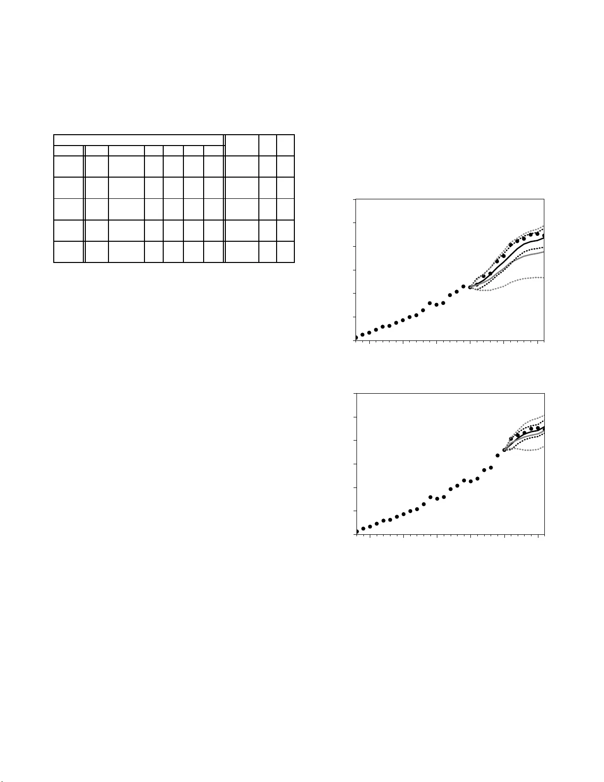
Mo delling recorded crime: a full searc h for coin tegrated mo dels J. L. v an V elsen Dutch Ministry of Just ic e, R ese ar ch and Do cumentation Cent r e (WODC), P. O. Box 20301, 2500 EH The Hague, The Netherlands ∗ A mod elgenerator is developed that searc h es for cointeg rated mo dels among a p oten tially large group of candidate mo dels. The generator employs the first step of the Engle-Granger pro cedure and orders coin tegrated mo d els according to th e informatio n criterions AIC and BIC. Assisted by the generator, a coin t egrated relatio n is established b etw een recorded violent cr ime in the Netherlands, the num b er of males aged 15-25 years (split into W estern and non-W estern background) and deflated consumption. In-sample forecasts reveal that the coin tegrated mo del outp erforms the b est short-run mod els. I. INTRO DUCTION The statistical relation b etw een reco rded crime and economic and demogra phic v aria ble s , such as unemploy- men t and the num b er of young males, is not o nly of fun- damental imp ortance [1 , 2, 3], but b ecomes increasing ly impo rtant in for ecasting to ols for policy and planning decisions [4, 5]. As recor de d crime and its pr edictor v a ri- ables are generally integrated o f or der o ne, tw o kinds of mo dels exist. There ar e short-run mo dels sp ecified in first differences and co in tegrated mo dels sp ecified in levels. In a short-r un mo del, crime has a strong sto chastic dyna mic of its own, even tually drifting a way uncontrollably from the relation with its predictors. Conv ersely , in a c o in te- grated mo del, crime fluctuates with constant v ar iabilit y around the re lation with its predicto rs, thereby preser v- ing its importa nce in the long run. As a cons e quence, cointegrated mo dels are to b e fav ore d over short-r un mo dels when making long ter m for e casts. Theor etically , given a set o f predictor v ar iables, one ca nnot arg ue c o n- clusively whether a cointegrated mo del applies. Empir- ically , howev er, a time series analysis indicates whether a cointegrated model is supp or ted b y the data or not [6, 7]. F or example, no cointegration was found b etw een crime and unemployment in England and W ales [1 ], while a cointegrated r elation was established b etw een robb ery rate and divorce rate in the United States [3]. The ob jective of this w o r k is to go b eyond a time ser ie s analysis for a fixed set of predictor v ariables. Rather, we consider a ll subsets of a set of p otential predictor v ari- ables and s earch for co in teg rated mo dels. The kind of crime under inv estig ation is vio le nt cr ime in the Nether- lands, co mp osed of ro bber y , as sault, ho micide, r ape and extortion. The set of p otential predictor v ar iables con- sists of unemplo yment , the n um ber of males aged 15-2 5 years of W estern background, the num b er of males ag ed 15-25 years of non- W estern background, the num b er of divorces a nd deflated co nsumption. A manual insp ec- tion o f a ll subsets is not feas ible b ecause the num b er of subsets, and thereby the num b er o f candidate mo dels, ∗ Electronic add ress: j.l.v an.velsen@minjus.nl grows ex p onentially with the num b er of p otential predic- tor v ar iables. E v en with five p otential predictor v ariable s and a llowing for a p otential erro r correction parameter, a constant or a constant a nd a trend, nearly tw o h un- dred c andidate mo dels exist. T o investigate these mo d- els, we developed a mo delgener ator that automatically builds and estimates them a nd subsequently chec ks for cointegration. The cointegration chec k consists of the first step of the Engle-Gra nger (E G) pro cedure [6]. The generator discards mo dels that ar e not co in teg rated a nd then estimates the cointegrated mo dels using NLS re- gressio n. Finally , the g enerator orders the cointegrated mo dels using the infor mation criterions AIC [8] and B IC [9]. II. MODELSTRUCTURE AND PRELIMINAR Y DA T A ANAL YSIS A necessary condition for the e x istence of a coin te- grated r elation is that all v aria bles inv olved ar e inte- grated of the s ame non-v anishing order. ADF tes ts [10] indicate that reco rded violent c r ime and its p otential pre- dictor v ariables do not reject one or more null hypo theses of a unit r o ot up to the 0.10 level. These tests were p er- formed on annual data ra nging fro m 1 9 78 to 2006 and the deta iled results are listed in T able I. W e a ls o p er- formed KP SS tests [1 1] that r everse the n ull h ypo thesis (a unit ro ot) and the alterna tive h y p othesis (stationa r - it y) of the ADF tes ts . The KPSS results are included in T able I. The probabilities of x 2 having a unit ro ot and of x 2 being sta tionary are a ll rather sma ll (see T a- ble I for the sy m b olic no tation of the v ariables). F ur ther analysis reveals that x 2 is more likely to b e integrated of order t wo than of order one. How ever, based on the joint picture emerging from T able I, we c onclude that all v ari- ables (including x 2 ) a r e integrated of order o ne. Having met the nec e ssary condition, the following coin tegrated mo del may exist y t = X i ∈ S β i x it + η t , where η t = ǫ t 1 − φ L and | φ | < 1 . (1) Here, t denotes discr ete time measured in years, S is a non-empty subset of the integer s et S 0 = { 1 , 2 , 3 , 4 , 5 } , 2 β i is the co efficient co nnecting x i to y a nd ǫ is Gaussia n white noise. The op erator L is the ba c kshift o p era tor retarding a v aria ble with one y ea r and the autoregressive noise η is stationa ry and causal with correlatio n length − 1 / ln | φ | measured in years. Mo del (1) may b e aug- men ted with a consta nt c or a co nstant and a trend c + δ t . T ABLE I: Results of ADF tests and KPSS tests on recorded violen t crime and its p otential predictor v ariables. The lag length of t he ADF tests is selected with BIC. The n umb ers in the ADF columns are th e p robabilities of the vari able ha ving a u n it root. The sub columns ‘0’, ‘C’ and ‘CT’ corresp ond to a random wa lk around, respectively , zero, a constant and a constant and a trend. The probabilities are b ased on finite- sample distributions of the DF statistic [12] of Ref. [13]. The KPSS tests are p erformed with the Bartlett kernel and th e data-based Newey-W est bandwidth selectio n p rocedure [14]. The num b ers in the KPSS sub columns ‘C’ and ‘CT’ are the probabilities of the va riable b eing stationary around, respec- tively , a constant and a constant and a trend. These prob- abilities are based on the asymptotic test statistics of Ref. [11]. v ariable ADF KPSS symbol desc ription 0 C CT C CT y recorde d viole nt crime 1.00 0.98 0.65 < 0 . 05 < 0 . 05 x 1 unemp lo yment (numbe r 0.63 0.02 0.00 > 0 . 10 < 0 . 10 of p ersons age d 15-65 y ears lo oking for a job) x 2 num b er of males 0.13 0.01 0.00 < 0 . 05 ≈ 0 . 10 aged 15-25 y e ars of W estern b ackground x 3 num b er of males 0.99 1.00 0.01 < 0 . 05 < 0 . 10 aged 15-25 y e ars of non-W este r n b ackground x 4 num b er of divorces 0.83 0.07 0.39 < 0 . 10 > 0 . 10 x 5 deflated consum ption 1.00 1.00 0.06 < 0 . 05 < 0 . 05 The relatio n b etw een the x i and y in mo del (1 ) is in- stantaneous. This seems too restrictive as mor e com- plicated tempo raneous relations are plausible. F or ex- ample, in modelling the unemploymen t-cr ime relatio n, lagged unemploymen t has been a rgued to influence cur - rent crime n um ber s fr om a motiv ationa l persp ective [15]. Indeed, such an effect has b een found in a short-r un mo del of vio len t crime (robber y excluded) [1]. Mathe- matically , this cor resp onds to β 1 being a tra nsfer function rather than a co efficien t. The transfer function would be a p olyno mial in L co rresp onding to the substitution β 1 → β 10 + β 11 L . Here, the co efficient β 10 < 0 co rre- sp onds to the instan ta ne o us effect of x 1 on y ar gued from the oppor tunit y p ersp ective. The co efficient β 11 > 0 cor- resp onds to the la gged influence of x 1 on y argued fro m the mo tiv ational p ersp ective [23]. T o find out whe ther our historical data con ta in evidence of such a tempor a- neous relation, we employ the Box-Jenkins metho dolo g y [16]. This consis ts of stationar iz ing x 1 and y b y differ- encing, prewhitening x 1 with an ARMA filter, applying the filter to the sta tionarized y and ins p ecting the co r- relogr am o f the prewhitened x 1 and the filter ed y . The correlo gram did not hav e any sig nificant lag structure , indicating that β 1 is a s c alar. Now we turn to the tem- po raneous relations betw een y and the remaining predic- tor v ariables. The v ariables x 2 and x 3 are based o n the age distribution of cr ime [17, 18]. Their impact on y is instantaneous, but ma y also hav e a la gged compo nen t based on the followin g argument. A relatively vio len t (non-violent) g roup of individuals that is within the age cohort at time t , but outside the cohort at time t ′ > t , may influence y t ′ such that it is larger (smaller) than ex- pec ted based on x 2 t ′ and x 3 t ′ . That is, β 2 and β 3 may b e transfer functions, and when they are, probably with a non-v anishing num b er o f ro ots in their denominators to capture the long term cor r elations. W e again emplo y the Box-Jenkins metho dology and find that β 2 and β 3 are scalars . Finally , x 4 is indicative of stra in in so ciety [3] and x 5 is imp o rtant from b oth the motiv ational ( β 5 < 0) and the o ppor tunit y p ersp ective ( β 5 > 0). Both v ar iables are assumed to impact y instantaneously , an assumption confirmed by a Box-Jenkins analysis . All v ar iables ar e left untransformed. T aking the lo ga- ritm of y a nd the x i carries the a dditiv e mo del (1) o ver int o a multiplicativ e one. The tra nsformed model with S = { j } takes the for m y t = x β j j t e η t , s uc h that y dep ends non-linearly on x j (if β j 6 = 1) and the v ar iability o f y de- pends on x j . T ra ces of these signa tures were not found in scatter plots of y and the x i . Also , in the Box-Jenkins analyses, all v ariables b ecame stationar y (up to the 0.10 level of the KP SS test with a co nstant) after differencing without first taking the loga ritm. This also holds fo r de- flated consumption, which, in con trast to consumption, do es not need to be transfor med prior to differencing. II I. THE MODELGENERA TOR The mo delgenerato r builds all mo dels based on the (2 5 − 1) non- e mpt y subsets of S 0 . P o ssibly augmented with a constant o r a constant and a trend, there are 3(2 5 − 1) candidate mo dels. In addition, the genera- tor consider s mo dels with restr iction η = ǫ (this cor re- sp onds to φ = 0) a nd mo dels without this r estriction. This brings the total num b er o f c a ndidate mo dels to 6(2 5 − 1) = 186 . The gener ator chec ks each mo del for cointegration and then order s the cointegrated mo dels according to information criterio ns . These tw o stages of op eration are describ ed b elow. A. Checking mo dels On multiplying b oth sides of Eq. (1) by (1 − φ L ) and subtracting (1 − φ ) y t − 1 , the mo del takes error correction (EC) form ∆ y t = X i ∈ S β i ∆ x t +( φ − 1) " y t − 1 − X i ∈ S β i x i ( t − 1) # + ǫ t . (2) 3 Here, ∆ = 1 − L is the difference op erator and the term with square brack ets is the EC term. The regr ession equation (2) is non- linear in its parameters β i (and p os- sibly a constant or a constant a nd a trend) a nd error correctio n parameter φ [24]. The fir st step of the EG pro cedure consists of e s timating the co efficients β i (and po ssibly a consta nt or a constant and a trend) with the restriction φ = 0. Due to the restriction, the reg ression is linear and OLS is use d. If a DF test on the res idua ls fails to reject the null h yp othesis o f a unit ro ot up to the 0.05 level acco rding to the asymptotic test statistics of Ref. [13], the gener ator co nsiders the tw o cor resp onding candidate models (the one with φ = 0 in the first place and the one without this restriction) not cointegrated a nd discards them. In the second step of the EG pro cedure, the ter m in square bra c kets in Eq. (2) is r eplaced by the lagg e d res id- uals o f the firs t step a nd the resulting equa tion is esti- mated by OLS. As co mputation time is not really an issue with a mo derate num b er of candidate mo dels, the gen- erator do es not employ the second EG step a nd rather solves Eq. (2) directly using a Mar quardt NLS a lgorithm. The alg orithm is assis ted by ana lytic deriv atives o f the squared re s iduals to φ a nd executed with a co efficient accuracy of 1 · 10 − 4 and a maximum num ber of 5 · 10 2 it- erations. After estimating the pa rameters, the generator insp e cts the r esiduals and discar ds all models that reject the n ull hypothesis of no seria l cor relation up to the 0.20 level of the Breusch -Go dfrey (BG) LM test [19, 20]. The BG LM test is p erformed with tw o la g s a nd pre-s ample residuals are set to zero. B. Ordering mo dels The infor mation criterions AIC and BIC take the form AIC = ln SSR + 2 N n , BIC = ln SSR + N ln n n . (3) Here, SSR is the s um of squa red residua ls o f the NLS estimation, N is the total num b er of estimated para me- ters and n is the sample size. Mo dels with smaller AIC – an e s timator of the cross-entropy b etw een the unknown op erating model and the candidate mo del, av eraged over the op erating mo del – a r e fav ored ov e r mo dels with la rger AIC. The same holds for BIC which is related to the p os- terior probability of a mo del as ∼ exp( − BIC / 2). In finite samples, AIC under estimates the av er a ged cross-entrop y and fav ors mo dels that are to o complex [21]. If n ≥ 8 such that ln n > 2 , B IC has a la rger p enalty term than AIC a nd fav or s s impler mo dels. Whic h of the tw o crite- rions is more a ppropriate for finite n ≥ 8 canno t b e said befo rehand and the generator employs b oth. IV. RESUL TS Out of the 18 6 candidate mo dels, the ge ner ator pro - duces 15 cointegrated mo dels. The top-6 o f b est mo dels according to AIC happ ens to co incide with that accor ding to BIC in the sense that they contain the same mo dels, but with a differe n t order ing. T he s e 6 mo dels, as well as the corr esp o nding evidence r atio’s (E R’s ), are listed in T able I I. ER is related to AIC and BIC as, resp ectively , exp( − (AIC − AIC min ) / 2) a nd exp( − (BIC − BIC min ) / 2). Here, AIC min (BIC min ) denotes the smallest AIC (BIC) out of the cointegrated mo dels. F or BIC, ER measures the r atio of a posterio r pr obability and the highes t p oste- rior pro babilit y . The r esults of T a ble I I indica te that all 6 mo dels cont ain the num b er of non- W estern males x 3 and deflated co nsumption x 5 . In co n trast, the num b er of div o rces x 4 do es not appea r in a n y of the coint egrated mo dels. In a n additiona l r un o f the g e nerator, we used ( x 2 + x 3 ) rather than x 2 and x 3 . The r eason for this is the follow- ing. Supp ose the unknown oper ating mo del contains the nu m be r o f ma les a ged 1 5-25 y ear s without distinguishing betw een W es tern and no n-W estern background. Then, mo dels con taining x 2 and x 3 unnecessarily require esti- mation o f b oth β 2 and β 3 , while in fa ct β 2 = β 3 . O ut of the 6 · 2 3 = 48 candidate mo dels containing ( x 2 + x 3 ), t wo ar e found cointegrated. Both mo dels hav e a larger AIC and BIC than mo dels I-VI and leav e the r esults of T able I I unaffected. T ABLE I I: Schematic listing of cointegrated models. The v ariables x i represent the p otentia l predictor va riables as listed in T able I. The symbol ‘X’ indicates inclusion of the correspondin g predictor v ariable (or constan t c , tren d t or er- ror correcti on parameter φ ) . The columns ‘ER AI C’ and ‘ER BIC’ hold, resp ectively , the ER ’s according to AIC and BIC. While the mo dels are ordered according to BIC, the num- b ers in brack ets in the column ‘ER AIC’ d enote their order according to AIC. The num b ers in the column ‘BG LM’ are the probabilities of the residuals having no serial correlation according to the BG LM test. The col umn ‘EG DF’ holds the DF statistics of the OLS residuals of th e first step of the EG proced ure and th e numbers in brack ets are the corresp on d ing asymptotic test statistics at th e 0.05 level of Ref. [13]. mo del ER ER BG EG DF num b er c t x 1 x 2 x 3 x 4 x 5 φ AIC BIC LM I X X X 0.99 (3) 1. 00 0.38 -3.92 (-3.74) II X X X X 1.00 (2) 0.99 0.37 -4.41 (-4.10) II I X X X X X 1.00 (1) 0.97 0.35 -4.67 (-4.43) IV X X X X 0. 96 (6) 0.95 0.84 -3.92 (-3.74) V X X X X X 0.98 (4) 0.94 0.35 -4.48 (-4.43) VI X X X X X 0.97 (5) 0.94 0.37 -4.49 (-4.41) T o inv estigate the co in tegration str uc tur e of mo dels I- VI, we co nsider the VEC (vector err or corr ection) models ∆ z t = ( α  γ + β T z t − 1  + µ t (a) α  γ + δ t + β T z t − 1  + α ⊥ δ ′ + µ t . (b) (4) Here, z is the 5-dimensional column vector ( y , x 1 , x 2 , x 3 , x 5 ) T and ‘T’ denotes the tr ansp o se of a matrix o r vector. The matr ices α and β a r e 5 × r matrices, where r ≤ 4 is the cointegration rank. The 4 5-dimensional columnv ector µ is Gaussian white noise with 5 × 5 cov a riance matrix Ω. The r -dimensio nal columnv ector γ holds constan ts within the EC terms α  γ + β T z t − 1  and α  γ + δ t + β T z t − 1  . Similarly , the r -dimensio nal co lumn vector δ holds prefac to rs of the trend t inside the EC term α  γ + δ t + β T z t − 1  . The (5 − r )-dimensional co lumn vector δ ′ corres p onds to trends in the columnspace of the 5 × (5 − r ) ma trix α ⊥ satisfying α T α ⊥ = 0. The difference betw een the VEC mo del (4) and the EC mo del (2) is that the latter describ es the dynamics of y only , while the former describ es the join t dynamics o f y and ( x 1 , x 2 , x 3 , x 5 ). The corr espo ndence b etw een the VEC mo del and the EC model is, that, conditioned on ( x 1 , x 2 , x 3 , x 5 ), the sto chastic pr o ce s s of y implied by the VEC mo del takes the form of the EC mo del [25]. W e first consider mo dels I, I I, IV, VI and p erform a Johansen cointegration test [7 ] to find r , α , β and γ of VEC mo del (a) without trends. Up to the 0.05 level o f Ref. [22], the trac e test indicates r = 3 (LR = 0.065) and the maximum eigenv alue test indicates r = 4 (LR = 0.022). W e acce pt r = 4 . This means that ther e is only one common non-stationa r y signal and the 4 linear com- binations corr espo nding to the ele men ts o f β T z a re such that this s ignal is ca ncelled. T o see if this agr ees with an EC model, we try to find co efficients ξ i such that P 4 i =1 ξ i ( β β β T i , γ i )( z T , c ) T equals the EC term of the EC mo del. Here, β β β i denotes the i -th column of β . Indeed, for each EC mo del, a set of co efficients { ξ i } exists within error b ounds o f a standard devia tion ab ov e and below the estimated par a meters. Now we turn to mo dels I I I, V and find r , α , β , γ a nd δ o f VEC mo del (b) with trends. Up to the 0.05 lev el, b oth the trace test and the maximum eigenv a lue test indicate r = 3, with, resp ectively , LR = 0.079 and LR = 0.063 . In this case, we search fo r co- efficients ξ i such tha t P 3 i =1 ξ i ( β β β T i , γ i , δ i )( z T , c, t ) T equals the EC term of an EC mo del. It turns out that, for b oth mo dels, s ets o f co efficients { ξ i } do no t exist within err or bo unds. In o ther words, mo dels II I, V are not cons isten t with the VEC mo del at the 0.05 level and we discard them. The estimated parameters of mo dels I, II, IV, VI a r e listed in T a ble I I I. The estimated par ameter of x 1 in mo del VI is insignificant. The same holds for the EC parameter φ in mo del IV. As it do es not ho ld x 2 , mo del I is less pla usible than mo del I I. W e conclude that model II is the b est co in teg rated mo del. V. A COMP ARISON WITH SHOR T-RUN MODELS In Sec. IV, only 1 5 cointegrated mo dels w ere fo und out of 1 86 candidate mo dels sp ecified in levels. This mea ns that for many subsets S , the proper mo del sp ecification is in first differences rather than in levels. W e therefore T ABLE I I I: Estima ted parameters and t-ratio’s (in b rac kets) of mod els I, I I, I V, VI of T able I I. mod el num b er c · 10 3 x 1 · 10 − 3 x 2 · 10 − 2 x 3 · 10 − 2 x 5 a φ I − 59 31 . 1 0 . 37 ( − 10 . 2) (5 . 3) (8 . 0) I I − 89 1 . 5 28 . 3 0 . 44 ( − 4 . 6) (1 . 6) (4 . 7) (7 . 0) IV − 57 33 . 2 0 . 35 0 . 26 ( − 7 . 2) (3 . 9) (5 . 4) (1 . 2) VI − 95 3.2 1 . 5 23 . 7 0 . 47 ( − 4 . 0) (0.5) (1 . 6) (2 . 1) (4 . 8) a expressed in mil lions of euros deflated wi th r espect to the year 2000 consider the shor t-run mo del ∆ y t = X i ∈ S β i ∆ x it + ǫ t . (5) Mo del (5 ) may be a ugment ed with a constant and when it is, S may the empt y set. The genera tor is used to find the b est out of the 2 6 − 1 = 6 3 short- run mo dels. (The cointegration chec k is switched off and the mo dels ar e estimated with O LS.) The gene r ator finds 51 mo dels with a BG LM proba bilit y of no s e rial corr elation exceeding 0.20. The top-5 models a ccording to BIC ar e listed in T able IV. Mo dels I and IV ar e equal up to an insig nificant constant in mo del IV. Mo del I I ho lds only ∆ x 3 and is considered too simple. The c o efficient of ∆ x 1 in mo del V is insignificant and we co nclude that mo dels I a nd I I I are the b est shor t-run mo dels. In an additional run of the ge ne r ator, we used ∆( x 2 + x 3 ) ra ther than ∆ x 2 and ∆ x 3 . Out of the 16 candidate mo dels containing ∆( x 2 + x 3 ), the g enerator selects 14 mo dels. All these mo dels have a larger AIC and BIC than mo dels I- V and leav e the results of T a ble IV unaffected. The predictive p ow er of sho r t-run models I and I I I is compar ed to that of co in tegrated mode l I I by in- sample for ecasts. The outcome o f the comparis on is not known beforehand: x 4 may be a go o d predictor of y a nd the short-run models ca n outp erfor m the co in teg rated mo del when mak ing shor t term for ecasts. W e mak e a long (short) term forecast, e s timating the mo dels using data from 1978 up to 19 95 (20 00) and for ecasting them from 1996 (20 01) to 2 006. The fore c asts ar e bas ed on a Monte Carlo simulation of 10 4 rep etitions (including co- efficient uncer ta in t y) and consist of mean for e casts a nd error b ounds. The results for shor t-run mo del I and the cointegrated mode l are indicated in Fig. 1. Panel (a) holds the long ter m for e c asts and indicates that the coin- tegrated model o utper fo rms the sho rt-run mo del in the sense that its mean pr edictions ar e closer to the rea liza- tions and that its error bounds a re smaller. In panel (b), holding the sho rt term fore casts, the mean for ecasts of the mo dels ar e very similar , but the error b ounds of the 5 T ABLE IV : Estimated parameters and t- ratio’s (in brack ets) of the top-5 short- run mo dels according to BIC. The columns ‘ER AIC’ and ‘ER BIC’ hold, resp ectively , th e ER ’s according to A I C and BIC. The n umb ers in brack ets in the column ‘ER AIC’ denote the rank ing according to A I C. The column ‘BG LM’ holds the probabilities of the residuals ha v ing no serial correlation according to the BG LM test. mo del ER ER BG num b er c ∆ x 1 · 10 − 3 ∆ x 2 ∆ x 3 ∆ x 4 ∆ x 5 AIC BIC LM I 0.36 0.46 0.29 1.00 (1) 1.00 0.39 (2.9) (2.0) (2.7) II 0.62 0.91 (18) 0.95 1.00 (6.2) II I -17 0.65 0.48 0.95 (5) 0.95 1. 00 (-2.0) (6.7) (2.0) IV - 464 0.41 0.48 0.32 0.97 (2) 0.95 0.25 (-0.4) (2.3) (2.0) (2.3) V − 3 . 2 0.39 0.47 0.26 0.97 (3) 0.94 0.39 (-0.3) (2.2) (2.0) (1.7) short-run mo del are larger. The forecasts of short-r un mo del I II are similar to that of short- run mode l I. In panel (a), short-r un model I I I would pro duce mean fore - casts a bit w o rse than that of short-r un mo del I. In panel (b), it would pro duce mean for ecasts a bit closer to the realizations than that of shor t-run model I and the coin- tegrated model. The er ror b ounds of short-run model I II are compar able to that of shor t-run mo del I. VI. CONCLUSIONS W e hav e develope d a mo delgener ator that searches for cointegrated mo dels among candidate mo dels specified in levels. The gener a tor employs the first step of the EG pro cedure to dec ide whether a mo del is cointegrated or not. Subsequen tly , it estimates the coin tegrated mo dels with NLS regre s sion and chec ks the residuals with the BG LM test. Finally , it o rders mo dels acco rding to b oth AIC a nd BIC. The gener ator is applied to recorded v io - lent cr ime and five p otent ial predictor v ariable s : unem- ploymen t, the num b er of males ag ed 15-2 5 years of W es t- ern ba c kground, the nu m be r of males aged 15- 25 y ears of non-W ester n ba c kground, the num b er of divorces and deflated consumption. The pattern emerging from the ordered list o f coint egrated mo dels is tha t the num b er of males ag ed 15-25 years of non-W estern bac k g round and deflated consumption ar e the k ey predictors o f r ecorded violent crime. Based on an analy s is of VEC mo dels, a plausibility a rgument and the statistical significance of estimated parameters , we select a cointegrated mo del out of the o rdered list. The selected mo del holds, in addition to the key predic to rs, the nu mber of males aged 15-25 years of W ester n background. With the cointegration chec k switc hed off, the gener- ator is used to find short-r un models spec ifie d in first differences. The key predictors of the sho rt-run models are the n umber of ma le s aged 15-25 years of non-W estern background a nd the n umber of divorces. Based on a plausibility a rgument and the statistical significance of estimated par ameters, t wo short-run models are selected from the order e d list. In addition to the key predictors, one of the shor t-run mo dels holds deflated co ns umption and the other unemploymen t. In-sample forecasts reveal that the co in tegrated mo del o utper fo rms the tw o short- run mo dels in b oth mea n predictions (long term) and error bo unds (long term and short term). 20 40 60 80 100 120 140 1980 1985 1990 1995 2000 2005 t y/1000 (a) 20 40 60 80 100 120 140 1980 1985 1990 1995 2000 2005 t y/1000 (b) FIG. 1: Realizations (blac k dots) and mean forecasts of coin- tegrated model I I of Sec. IV (solid black lines) and short-run mod el I of Sec. V (solid gray lines). The dashed black (gra y ) lines constitut e error b ounds of tw o stand ard deviations ab o ve and below the mean forecasts of the cointeg rated (short-ru n) mod el. In p anel (a), the mo dels are estimated based on re- alizations from 1978 up to 1995 and forecasted from 1996 u p to 2006. In panel (b), the mo dels are estimated based on re- alizations from 1978 up to 2000 and forecasted from 2001 u p to 2006. 6 [1] C. Hale and D. S abbagh, Journal of R esearch in Crime and Delinquency 28 , 400 (1991). [2] C. L. Britt, American Journal of Economics an d So ciol- ogy 53 , 99 (1994). [3] D. F. Greenb erg, Journal of Quantitativ e Criminology 17 , 291 (2001). [4] R. Harries, International Journal of F orecasting 19 , 557 (2003). [5] D. Deadman, International Journal of F orecasting 19 , 567 (2003). [6] R. F. Engle and C. W. J. Granger, Econometrica 55 , 251 (1987). [7] S. Johansen, Jo urnal of Economic Dynamics and Control 12 , 231 (1988). [8] H. Ak aike, in 2nd International Symp osium on Infor- mation The ory , edited by B. N. Petro v and F. Csaki (Ak ademia Kiado, 1973). [9] G. S c hw arz, Annals of Statistics 6 , 461 (1978). [10] S. E. Said and D. A. Dick ey , Biometrik a 71 , 599 (1984). [11] D. Kwiatko wski, P . C. B. Phillips, P . Schmidt and Y. Shin, Journal of Econometrics 54 , 159 (1992). [12] D. A. Dic key and W. A. F uller, Journal of the American Statistical Asso ciation 74 , 427 (1979). [13] J. G. MacKinnon, Journal of Ap plied Econometrics 11 , 601 (1996). [14] W. K. Newey and K. D. W est, R eview of Economic Stu d - ies 61 , 631 (1994). [15] D. Can t or and K. C. Land, American So ciologi cal Review 50 , 317 (1985). [16] G. E. P . Bo x and G. M. Jenkins, T ime Series A nalysis: F or e c asting and Contr ol (Holden-Day , 1976). [17] T. Hirschi and M. Gottfredson, American Journal of So- ciology 89 , 552 (1983). [18] D. J. Steffensmeier, E. A . Allan, M. D. Harer an d C. Streifel, American Journal of So ciology 94 , 803 (1989). [19] T. S. Breusch, Australian Economic Papers 17 , 334 (1978). [20] L. G. Godfrey , Econometrica 46 , 1293 (1978). [21] C. M. Hurvich and C. - L . Tsai, Biometrik a 76 , 297 (1989). [22] J. G. MacKinnon, A. A. Haug and L. Michelis, Journal of Ap p lied Econometrics 14 , 563 ( 1999). [23] The signs of β 10 and β 11 do not alwa ys agree with emp iri- cal findings. F or example, in Ref. [3], several cointegrated mod els w ere t ried, all indicating β 11 < 0. In addition, th e short-run mo del of robb ery of Ref. [1] has β 10 > 0 and β 11 < 0. [24] The constant c and tren d δ t that can b e augmented to Eq. (1), carry ove r to t h e EC term. In addition, δ t app ears as δ φ outside the EC term. [25] Rephrased in terms of the n oise pro cess η and transfer functions β i ( L ), the conditional dynamics of y implied by (4) is more general than (2) as it allo ws for a ratio- nal β i ( L ) with numerator ( β i 0 + β i 1 L ) and d enominator (1 − φ L ). In the EC mo del, th is corresponds to different coefficients inside and outside the EC term.