On the Capacity and Generalized Degrees of Freedom of the X Channel

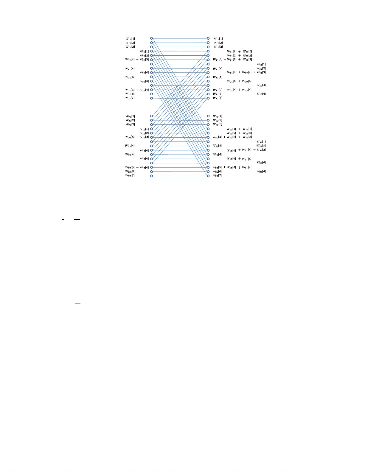
1 On the Capacity and Generalized De grees of Freedom of the X Channel Chiachi Huang, V iv eck R. C adambe, and Syed A. Jafar Electrical Engineering and Computer Science Univ ersity of California Irvi ne Irvine, California, USA Email: { chiachih, v cadambe, syed } @u ci.edu Abstract W e explore the capacity and g eneralized degrees of fr eedom of the two-user Gau ssian X channel, i.e. a generalizatio n of the 2 user interferen ce channel where there is an in depend ent message from each transmitter to each receiver . There are three main results in this paper . First, we characterize th e sum capacity of th e d eterministic X channel model under a symmetric setting. Second, we characterize the generalized degrees of freedom of the Gaussian X channel under a similar symmetric model. Third, we extend the noisy inte rference capacity characterizatio n previously obtained for the interferen ce channel to the X channel. Specifically , we sho w that the X chan nel as sociated with noisy ( very weak) interfe rence c hannel has the same sum capacity as the noisy interferenc e channel. 2 I . I N T RO D U C T I O N Recent rese arch in multi- user information theory h as b een cha racterized by a sur ge of interest in the study of capac ity regions of wireless Ga ussian networks. Much of this interes t has been fueled by sign ificant recent progres s in the search of the capacity region of wireless interference networks, a classical problem of multi-user information theory . In their s eminal work [1], Etkin, Ts e and W ang approximated the capacity region o f the two-user Gaussian interference channel to wit hin one bit. Further insight into the ca pacity of the t wo-user Gaussian interf erence network was re vealed in [2]–[4]. Thes e references found that the decoding strategy of treating interferenc e as noise at each receiv er in the interference n etwork is capa city optimal for a clas s of interferenc e ch annels, known as the “no isy interference” c hanne ls. Re cent res ults have also found approximations to the capa city regions of certain class es of the K -user interf erence channe l in the high signal-to-noise ratio (SNR) regime. Referenc e [5] approximated the capac ity region of the fully c onnec ted K -user interference channel with time-varying chan nel coe f ficients a s C ( SNR ) = K 2 log( SNR ) + o (log( SNR )) where SNR represents the total transmit power of all node s when the local noise po wer at each recei ver is no rmalized to unity . In o ther words, it was shown that the time-varying K -user interference c hannel has K 2 degrees of freedom. Similar capac ity approx imations of the K -user ( K > 2 ) interference channe l with co nstant channel c oefficients (i.e., not time-varying o r frequency-selecti ve) are not known in general. From the recent advances in the study of interference channe ls, many interesting and powerful tools related to the study of ge neral wireless networks have eme r ged. Referen ce [1] introduced the notion of generalized degr ees of fr eedom to study the p erformance o f v arious inte rference management sche mes in the interference c hannel. As its name s ugges ts, the ide a of gen eralized degrees of freedom is a generalization of the concep t of degrees of freedom originally introduc ed in [6]. The idea of generalized degrees of freedom is powerf ul bec ause in the multiple acce ss, broadcas t a nd two-user interferenc e ch annels, achiev able schemes that are optimal from a gene ralized degrees of freed om pe rspectiv e also achiev e within a c onstant n umber o f bits of ca pacity [7]. A u seful tech nique in the characterization of the generalized degrees of freed om of a wireless n etwork is the d eterministic approach , originally introduced in the c ontext of relay ne tworks [8]. The deterministic ap proach esse ntially maps a Gauss ian network to a deterministic chan nel, i.e, a channe l whose outputs a re deterministic functions of its inputs. Th e deterministic channe l captures the ess ential structure of the Ga ussian cha nnel, but is significa ntly simpler to analyze. Re ference [7] showed that the deterministic approach leads to a characterization of the gen eralized degrees of freedom of wireless networks in the two-user interference network, which leads to a constan t bit approximation of its capacity . In this paper , we explore the two-user X channel - a ne twork with two transmitters, tw o rec eiv ers and four independ ent message s - one correspon ding to e ach transmitter-recei ver pair . The d egrees of freedom of the Ga ussian X channel h av e been found in [ 9], [10]. This work pursues a more refined characterization in terms of the generalized degrees of free dom. Unlike the co n ventional degrees of freedom pe rspective where a ll signals are approx imately equally strong in the dB scale, the ge neralized degrees of freedom perspe cti ve provides a richer characterization by allowi ng the full range of relati ve signal strengths in the dB sc ale. For example, consider the interference chann el. The strong an d weak interferenc e s cenarios are not visible in the co n ventional degrees of freedom perspective but b ecome immediately obvious in the generalized degrees of freedo m framew ork. No w consider the X ch annel which is a ge neralization of the interference channel to a scena rio where every trans mitter ha s a message to e very receiv er . One of the key fe atures of the X channe l is that, unlike the two-user interf erence channe l, it provides 3 Y 2 Y 1 Z 2 Z 1 X 2 W 12 , W 22 W 11 , W 21 X 1 ˆ W 21 , ˆ W 22 ˆ W 11 , ˆ W 12 Fig. 1. The two-user Gaussian X channel the pos sibility of interference alignment [9], [10]. Interf erence a lignment refers to the co nstruction of s ignals s uch that they overlap a t receivers where they cause interference, b ut remain distinguishab le at receivers where they are desired. Interference alignment is the key to the degrees of freedom characterizations of the X channe l with 2 or more users [11], and for the interference channe l with 3 or more use rs [5]. Since the potential for interference alignment doe s not arise in the 2 user interference ch annel, the two-user X channel provides the simplest po ssible setting for interferenc e a lignment, in terms of the n umber of transmitters/receiv ers and chan nel co efficients. It is shown in [10] that, due to interference alignment, the 2 user X c hannel ha s 4 / 3 degrees of freedom (assuming time- varying cha nnels), wh ile the 2 user interference c hanne l ha s only 1 d egree of freedom. In this work, we explore this capac ity advantage of the X cha nnel over the interference channe l in the richer context o f the gen eralized degrees of freedom. Spe cifically we quantify the benefi ts of interference alignment in terms of ge neralized degrees of freedom and identify op erating regimes where alignment helps the X c hanne l outperform the interference channel. For simplicity , we will keep the number of ch annel parameters to a minimum by us ing the symme tric interference channe l as our benchmark and presenting our main results for the corresp onding s ymmetric X channel. Our a pproach to solving the generalized degrees of freedom of the X cha nnel follo ws the d eterministic approa ch of [12]. W e first introdu ce the deterministic X channe l, a nd find a tight o uterbound and ach iev able sche me for the sum cap acity of this chann el in Section IV. In Sec tion V, we extend the ach iev ability and outerbound arguments of Sec tion IV to the Gaussian X channe l yielding its generalized degrees of freedo m. A se cond result we obtain is a gene ralization of the results of [2]–[4] to fi nd the ca pacity of the Gauss ian X chann el for a class of cha nnel coefficients. W e introduce the system model, formally define the notion of generalized degrees of fr eedom, and present the main results in the next section. I I . S Y S T E M M O D E L A. Deterministic X Channel The deterministic X c hanne l is phys ically the s ame channe l as the deterministic interference cha nnel introduce d in [7], except tha t the X chan nel ha s 4 independ ent mess ages { W 11 , W 12 , W 21 , W 22 } where W ij is the mess age that originates at transmitter j an d is intended for rec eiv er i . Note that the interference cha nnel has only 2 inde penden t messag es, e .g., { W 11 , W 22 } or { W 12 , W 21 } . The deterministic chann el is sho wn is Fig. 2 and described by the 4 Tx 1 Tx 2 Rx 1 Rx 2 Rx 1 Rx 2 1 2 1 2 n 11 n 12 n 22 n 21 Fig. 2. On the left is an ex ample of the deterministic interference chann el. On the right is the figure that sho ws only the signal leve ls observ ed at each receiv er . input output eq uations Y 1 ( t ) = S q − n 11 X 1 ( t ) + S q − n 12 X 2 ( t ) (1) Y 2 ( t ) = S q − n 21 X 1 ( t ) + S q − n 22 X 2 ( t ) (2) where q = max( n 11 , n 21 , n 12 , n 22 ) , X i ( t ) , Y i ( t ) ∈ F q 2 for i = 1 , 2 , an d S is a q × q s hift matrix, S =          0 0 0 · · · 0 1 0 0 · · · 0 0 1 0 · · · 0 . . . . . . . . . 0 0 0 · · · 1          (3) The messa ge set and stan dard definitions and n otations of the a chiev able rates are similar to thos e in the Ga ussian setting. T o avoid confusion, sometimes we add the s ubscript det to distinguish the notations for the deterministic channe l from those for the Gaussian channel. B. The Gaussian X Channel The tw o-user Gaussian X channel is des cribed by the input-output e quations Y 1 ( t ) = H 11 X 1 ( t ) + H 12 X 2 ( t ) + Z 1 ( t ) (4) Y 2 ( t ) = H 21 X 1 ( t ) + H 22 X 2 ( t ) + Z 2 ( t ) (5) 5 where a t symb ol index t , Y j ( t ) and Z j ( t ) are the cha nnel output symbol and additi ve white Gau ssian noise (A WGN) respectively at receiv er j . X i ( t ) is the cha nnel input s ymbol at trans mitter i , and H j i is the channe l g ain coe f ficient between transmitter i and receiver j for all i, j ∈ { 1 , 2 } . All symbols are real and the channel coefficients do not vary w .r .t symbo l index. In the remainder of this paper , we suppress time index t if n o c onfusion would be cau sed. The A WGN is no rmalized to have zero mean and unit v ariance and the input power constraint is given by E  X 2 i  ≤ P i , i = 1 , 2 . (6) There are four independe nt me ssage s in the X channel: W 11 , W 12 , W 21 , W 22 where W ij represents the message from transmitter j to rece i ver i . W e indicate the s ize of the message by | W ij | . For codewords s panning T sy mbols, rates R ij = log | W ij | T are a chiev able if the prob ability of error for a ll mes sages can b e simultaneou sly made a rbitrarily small by choosing an a ppropriate lar ge T . The c apacity region C of the X channel is the set of all achiev able rate tuples R = ( R 11 , R 12 , R 21 , R 22 ) . W e indicate the sum cap acity of the X channel b y C Σ . 1) Generalized De gr ees of F r eedom (GDOF): T o moti v ate our prob lem formulation, we briefly revisit the framew ork for the generalized degrees of freedom characteriza tion of the symmetric interference channe l. The interference channel is defin ed as : Y 1 ( t ) = √ SNR X 1 ( t ) + √ INR X 2 ( t ) + Z 1 ( t ) (7) Y 2 ( t ) = √ INR X 1 ( t ) + √ SNR X 2 ( t ) + Z 2 ( t ) (8) and with the parame ter α defined as follows α , log( INR ) log( SNR ) (9) the GDOF metric is defined as [1], d ( α ) = lim sup SNR →∞ C Σ ( SNR , α ) 1 2 log( SNR ) (10) where C Σ ( SNR , α ) is the s um capacity of the interference c hanne l. Since our main goal is to compare GDOF of the X channel with the interference channel, w e use the same symmetric interf erence channel model described above as the p hysical cha nnel model for the X chann el. There is h owe ver , on e no tational difference. Since the terminology SNR , INR is not as appropriate for the X chan nel, we instead use the paramete r ρ to substitute for these notions, resulting in the follo wing system model for the X channe l GDOF characterization: Y 1 ( t ) = √ ρX 1 ( t ) + √ ρ α X 2 ( t ) + Z 1 ( t ) (11) Y 2 ( t ) = √ ρ α X 1 ( t ) + √ ρX 2 ( t ) + Z 2 ( t ) (12) In other words, we have se t H 11 = H 22 = √ ρ , H 12 = H 21 = √ ρ α , an d P 1 = P 2 = 1 . Note that (11), (12) represent the same phy sical chann el a s (7), (8). Howev er , as mentioned earlier , un like the interference c hanne l the X c hanne l has 4 indepe ndent me ssage s - one from each transmitter to each receiv er . The GDOF charac terization for the X ch annel is defin ed as : d ( α ) = lim s up ρ →∞ C Σ ( ρ, α ) 1 2 log( ρ ) (13) 6 where C Σ ( ρ, α ) is the su m c apacity of the X cha nnel. Note that we use lim su p to en sure tha t d ( α ) a lw ays exits. The half in the de nominator is beca use all signals and channel g ains are real. I I I . M A I N R E S U LT S A. Sum Capacity o f the Sy mmetric Deter ministic X Channel The first main resu lt of the pap er is the characterization of the sum cap acity of the symmetric deterministic X channe l in the s ymmetric s etting where n 11 = n 22 = n d and n 12 = n 21 = n c . Th is result is giv en in the follo wing theorem. Theorem 3.1: The sum cap acity C Σ ( n c , n d ) of the s ymmetric deterministic X channel, i.e., the deterministic X channe l where n 11 = n 22 = n c and n 12 = n 21 = n d , is C Σ ( n c , n d ) =                            2 n d − 2 n c , 0 ≤ n c n d < 1 2 2 n c , 1 2 ≤ n c n d < 3 4 2( n d − 1 3 n c ) , 3 4 ≤ n c n d < 1 n d , n c = n d 2( n c − 1 3 n d ) , 1 < n c n d ≤ 4 3 2 n d , 4 3 < n c n d ≤ 2 2 n c − 2 n d , n c n d > 2 (14) B. Generalized De grees of F reedom of the Symmetric Gaussian X Channel The s econd main res ult of this pa per builds upo n the result of Theo rem 3.1 to fin d the g eneralized degrees of freedom characterization (shown in Figure 3) for the Gaussian X chann el. Theorem 3.2: The generalized degrees of fr eedom d ( α ) of the symme tric Gau ssian X c hanne l can be charac - terized as d ( α ) =                            2 − 2 α, 0 ≤ α < 1 2 2 α, 1 2 ≤ α < 3 4 2 − 2 3 α 3 4 ≤ α < 1 1 α = 1 2 α − 2 3 1 < α ≤ 4 3 2 4 3 < α ≤ 2 2 α − 2 α > 2 (15) For compa rison, Figure 3 also sh ows the gene ralized degrees of freed om cha racterization of the symmetric interference c hanne l as obtained in [1]. For values of α < 2 / 3 , cha racterization of d ( α ) is ide ntical for both the symmetric two-user Gaussian X channe l and the symme tric two-user Gaus sian interferenc e chann el (See [1] Figure 4.5). W e prove this by showing tha t the E tkin-Tse-W a ng (ETW) outerbo und d eri ved for the interference cha nnel [1] holds for the X channel as well (See T heorem 5.3). Th e ETW outerbou nd is tight from a GDOF persp ectiv e in the interf erence c hanne l for α ≤ 2 / 3 . Therefore, our extension of this outerbou nd implies tha t for α ≤ 2 / 3 a GDOF optimal achiev able sc heme is to set W 12 = W 12 = φ , so that the X channel op erates as an interference channe l. For example, if α ≤ 1 / 2 , s etting W 21 = W 12 = φ a nd treating interference as noise is GDOF optimal in the X chan nel, since it is optimal in the correspon ding interference cha nnel [1]. Similarly , we s how tha t for α > 3 2 , 7 1 3 1 2 2 3 4 2 1 4 3 5 2 4 3 3 2 ! ( ) d ! GDOF o f interferen ce channel obtain ed by W 12 = W 21 = ! GDOF o f the X channel Fig. 3. Generalized Degrees of Freedom of the symmetric X channel, and a comparison the the 2 user interference channel it is GDOF o ptimal to s et W 22 = W 11 = φ and ope rate the X channel as an interference channe l with message s W 12 and W 21 . It mus t be noted that for both α ≤ 2 / 3 and α > 3 / 2 the GDOF optimal achiev able scheme operates the X channel as weak interference ch annel by setting the a ppropriate messag es to null. For 2 / 3 < α ≤ 3 / 2 , we propose an interference alignment b ased a chiev able scheme for the X channe l. T hus, in this regime, the X ch annel performs better tha n the interference channel by exp loiting the possibility of interference alignment. C. Capacity of the “Noisy ” Gaus sian X Channel References [2]–[4] s howed that in the interference channe l, for a cla ss o f channel coefficients, encoding me ssage s using Gaussian codebooks an d decoding de sired messages by treating interference as noise at each rec eiv er is capac ity optimal. Our las t ma in result extends this con clusion to the X ch annel as well. W e show that if a 2 user interference chan nel satisfies the n oisy interference c onditions obta ined in [2]–[4] then the co rresponding X channe l obtained by allowing all transmitters to communicate with all receivers, h as the s ame sum cap acity as the original noisy interference chann el. T his is a surprising res ult since it implies that for a clas s of X chann els, interference alignment has no capacity benefit. The res ult holds for the general (asymmetric) X channe l an d is stated as suc h in Theorem 6.1 in Section VI. For simplicity we re-state the result here for the sy mmetric case 8 ( H 11 = H 22 = 1 , H 12 = H 21 = h, P 1 = P 2 = P ) in a notation co nsistent with [4], as follo ws. Noisy “S ymmetric” X Channel Result: If   h  1 + h 2 P    ≤ 1 2 , then the sum capacity of the Gaussian X channel is given by C Σ = log  1 + P 1+ h 2 P  . Similarly , if | h | ≥ 2(1 + P ) the n the sum c apacity of the Gaus sian X c hanne l is given b y C Σ = log  1 + h 2 P 1+ P  . The condition   h  1 + h 2 P    ≤ 1 2 is the sa me as the n oisy interference condition in [4]. It mea ns that when the cross-links are too we ak, the re is no s um-capac ity benefi t in communicating messages over those links ( X channel operation), even thou gh it rules out interferenc e alignment, an d we a re better off just communicating on the direct links while treating the weak interference as noise. Thus , in this case messages W 12 , W 21 do not increase sum capac ity of the X channel. The other cond ition | h | ≥ 2(1 + P ) refers to a s trong cross-cha nnel s cenario. It says that when the cros s-links are too s trong relativ e to direct links , the n su m capa city is achieved by communicating only over the strong cross-links and treating the weak interference recei ved over the direct links as noise. In this case , mess ages W 11 , W 22 do not increase the s um c apacity of the X chan nel. Notation: In the rest of this pape r , we use the notation A ( T ) △ = ( A (1) , A (2) , . . . A ( T )) for any seque nce A . I V . S U M C A PAC I T Y O F T H E S Y M M E T R I C D E T E R M I N I S T I C X C H A N N E L The deterministic X channel mod el is des cribed in the symmetric s etting b y: Y 1 ( t ) = S q − n d X 1 ( t ) + S q − n c X 2 ( t ) (16) Y 2 ( t ) = S q − n c X 1 ( t ) + S q − n d X 2 ( t ) (17) where q = max( n c , n d ) . T o prove The orem 3.1, we use the following lemma. Lemma 4.1: C Σ ( n c , n d ) = C Σ ( n d , n c ) (18) The lemma follo ws tri vially from the sy mmetry in the X channe l. W e now proc eed to deri ve the con verse argument for Theorem 3.1. A. Upperb ounds In this sec tion, we start from the cap acity outerbounds for the (asy mmetric) deterministic X ch annel, and then we use the results to derive the c apacity outerbo unds for the s ymmetric setting. The following lemma provides a set of outerbou nds for the ach iev able rate tuple ( R 11 , R 21 , R 12 , R 22 ) of the (asymmetric) de terministic X c hanne l. Theorem 4.2: The a chiev able rate tuple ( R 11 , R 21 , R 12 , R 22 ) of the deterministic X chann el satisfies the follow- 9 ing inequalities. R 11 + R 12 + R 22 ≤ m ax ( n 11 , n 12 ) + ( n 22 − n 12 ) + (19) R 11 + R 21 + R 22 ≤ m ax ( n 21 , n 22 ) + ( n 11 − n 21 ) + (20) R 11 + R 21 + R 12 ≤ m ax ( n 11 , n 12 ) + ( n 21 − n 11 ) + (21) R 21 + R 12 + R 22 ≤ m ax ( n 21 , n 22 ) + ( n 12 − n 22 ) + (22) R 11 + R 21 + R 12 + R 22 ≤ m ax  n 12 , ( n 11 − n 21 ) +  + m ax  n 21 , ( n 22 − n 12 ) +  (23) R 11 + R 21 + R 12 + R 22 ≤ m ax  n 11 , ( n 12 − n 22 ) +  + m ax  n 22 , ( n 21 − n 11 ) +  (24) Pr oof: The bound on R 11 + R 12 + R 22 , (19), is proved by a genie upperbound. Con sider a genie-aide d cha nnel whe re a genie provides S q − n 12 X 2 , W 12 , and X 1 to recei ver 2 . For a block len gth T , we can bound R 22 as follo ws. T ( R 22 − ǫ ) ≤ I  W 22 ; Y 2 ( T ) , S q − n 12 X 2 ( T ) , W 12 , X 1 ( T )  (25) = I  W 22 ; X 1 ( T )  + I  W 22 ; Y 2 ( T ) , S q − n 12 X 2 ( T ) , W 12 | X 1 ( T )  (26) = I  W 22 ; S q − n 22 X 2 ( T ) , S q − n 12 X 2 ( T ) , W 12  (27) = I  W 22 ; S q − n 22 X 2 ( T ) , S q − n 12 X 2 ( T ) | W 12  (28) = I  W 22 ; S q − n 12 X 2 ( T ) | W 12  + I  W 22 ; S q − n 22 X 2 ( T ) | W 12 , S q − n 12 X 2 ( T )  (29) = H  S q − n 12 X 2 ( T ) | W 12  − H  S q − n 12 X 2 ( T ) | W 12 , W 22  + H  S q − n 22 X 2 ( T ) | W 12 , S q − n 12 X 2 ( T )  − H  S q − n 22 X 2 ( T ) | W 12 , S q − n 12 X 2 ( T ) , W 22  (30) = H  S q − n 12 X 2 ( T ) | W 12  + H  S q − n 22 X 2 ( T ) | W 12 , S q − n 12 X 2 ( T )  (31) where (27) and (28) hold becaus e all me ssage s are indepe ndent o f each other . (31) follows from the fact that X 2 is a function of W 12 , W 22 . Using Fano’ s inequality , R 11 + R 12 can be bo unded as follows. T ( R 11 + R 12 − ǫ ) ≤ I  W 11 , W 12 ; Y 1 ( T )  (32) = H  Y 1 ( T )  − H  Y 1 ( T ) | W 11 , W 12  (33) ≤ H  Y 1 ( T )  − H  Y 1 ( T ) | W 11 , W 12 , W 21  (34) = H  Y 1 ( T )  − H  Y 1 ( T ) | W 11 , W 12 , W 21 , X 1 ( T )  (35) = H  Y 1 ( T )  − H  S q − n 12 X 2 ( T ) | W 12  (36) Adding (31) an d (36 ), we have T ( R 11 + R 12 + R 22 − ǫ ) ≤ H  Y 1 ( T )  + H  S q − n 22 X 2 ( T ) | W 12 , S q − n 12 X 2 ( T )  (37) ≤ T  max ( n 11 , n 12 ) + ( n 22 − n 12 ) +  . (38) Letting T → ∞ ( ǫ → 0) , we prove (19). S imilarly , we can prove (20), (21 ), and (22). 10 Next, the first boun d on R 11 + R 21 + R 12 + R 22 , (23), can be proved a s follows. Consider a gen ie-aided ch annel where a genie provides S q − n 21 X 1 and W 21 to rec eiv er 1 . For a bloc k leng th T , using Fano’ s inequ ality , we c an bound R 11 + R 12 as the following. T ( R 11 + R 12 − ǫ ) ≤ I ( W 11 , W 12 ; Y 1 ( T ) , S q − n 21 X 1 ( T ) , W 21 ) (39) = I ( W 11 , W 12 ; Y 1 ( T ) , S q − n 21 X 1 ( T ) | W 21 ) (40) = I ( W 11 , W 12 ; S q − n 21 X 1 ( T ) | W 21 ) + I ( W 11 , W 12 ; Y 1 ( T ) | S q − n 21 X 1 ( T ) , W 21 ) (41) = H ( S q − n 21 X 1 ( T ) | W 21 ) − H ( S q − n 21 X 1 ( T ) | W 21 , W 11 , W 12 ) + H ( Y 1 ( T ) | S q − n 21 X 1 ( T ) , W 21 ) − H ( Y 1 ( T ) | S q − n 21 X 1 ( T ) , W 21 , W 11 , W 12 ) (42) = H ( S q − n 21 X 1 ( T ) | W 21 ) + H ( Y 1 ( T ) | S q − n 21 X 1 ( T ) , W 21 ) − H ( Y 1 ( T ) | S q − n 21 X 1 ( T ) , W 21 , W 11 , W 12 , X 1 ( T ) ) (43) = H ( S q − n 21 X 1 ( T ) | W 21 ) + H ( Y 1 ( T ) | S q − n 21 X 1 ( T ) , W 21 ) − H ( Y 1 ( T ) | W 12 , X 1 ( T ) ) (44) = H ( S q − n 21 X 1 ( T ) | W 21 ) + H ( Y 1 ( T ) | S q − n 21 X 1 ( T ) , W 21 ) − H ( S q − n 12 X 2 ( T ) | W 12 ) (45) Similarly , we h ave T ( R 21 + R 22 − ǫ ) ≤ H ( S q − n 12 X 2 ( T ) | W 12 ) + H ( Y 2 ( T ) | S q − n 12 X 2 ( T ) , W 12 ) − H ( S q − n 21 X 1 ( T ) | W 21 ) (46) Adding (45) an d (46 ), we have T ( R Σ − ǫ ) ≤ H ( Y 1 ( T ) | S q − n 21 X 1 ( T ) , W 21 ) + H ( Y 2 ( T ) | S q − n 12 X 2 ( T ) , W 12 ) (47) ≤ H ( Y 1 ( T ) | S q − n 21 X 1 ( T ) ) + H ( Y 2 ( T ) | S q − n 12 X 2 ( T ) ) (48) ≤ T  max( n 12 , ( n 11 − n 21 ) + ) + max( n 21 , ( n 22 − n 12 ) + )  . (49) Letting T → ∞ , we prove (23). Similarly , we can prove (24). After o btaining capacity outerbou nds for the deterministic X channe l, we u se them to deriv e su m-capacity upperboun ds for the symmetric cas e. Cor ollary 4.3: For any ach iev able sc heme, the s um-rate R Σ can be bo unded as R Σ ≤ R Σ ,up △ =                            2 n d − 2 n c , 0 ≤ n c n d < 1 2 2 n c , 1 2 ≤ n c n d < 3 4 2( n d − 1 3 n c ) , 3 4 ≤ n c n d < 1 n d , n c = n d 2( n c − 1 3 n d ) , 1 < n c n d ≤ 4 3 2 n d , 4 3 < n c n d ≤ 2 2 n c − 2 n d , n c n d > 2 11 Pr oof: Con sider any reliable coding sche me ach ieving sum rate R Σ . Then we can write R Σ ≤ 4 3 max ( n c , n d ) + 2 3 ( n d − n c ) + + 2 3 ( n c − n d ) + (50) R Σ ≤ 2 max ( n c , n d − n c ) (51) R Σ ≤ 2 max ( n d , n c − n d ) (52) Inequalities (51) and (52) are direct results o f (23) and (24). T o prove inequ ality (50), we do the following. Substituting n 11 = n 22 = n d and n 12 = n 21 = n c into (19) to (22), adding the res ulting inequalities together , an d divi ding both side s by 3 , we obtain (50). Further , for the symmetric deterministic X c hanne l, if n c = n d , then both rec eiv ers receive the s ame signa ls. Thus, the ac hiev able sum rate is bound ed by the multiple a ccess channel bou nd. R Σ ≤ n d (53) The result of Corollary 4.3 foll ows from (50)-(53). B. Achievable Schemes The follo wing the orem gi ves the sum c apacity o f the s ymmetric deterministic X c hannel. Theorem 4.4: The sum-capacity u pperbound g i ven in (4.3) is a chiev able. Equiv alently , C Σ ( n c , n d ) = R Σ ,up ( n c , n d ) (54) Before we proc eed to the proof, we will nee d the followi ng lemma Lemma 4.5: Let n c , n d be positi ve integers suc h that 3 4 ≤ n c n d < 1 . Then 1) If n c is di visible by 3 , then there exists a n d × n c 3 matrix V whose e ntries are from F n d 2 such that rank  V S n d − n c V S 2 n d − 2 n c V V null  = n d where V null is a n d × ( n d − n c ) whose column vectors form a basis for the nullspace of S n d − n c 2) There exists a 3 n d × n c matrix ¯ V whose entries a re from F 3 n d 2 such that rank  ¯ V ¯ H ¯ V ¯ H 2 ¯ V ¯ V null  = 3 n d where ¯ H =     S n d − n c 0 n d × n d 0 n d × n d 0 n d × n d S n d − n c 0 n d × n d 0 n d × n d 0 n d × n d S n d − n c     and ¯ V null represents the 3 n d × (3 n d − 3 n c ) matrix who se c olumn vectors form a basis for the nullspace of ¯ H The proof o f the lemma is placed in Appen dix II. W e now procee d to prove Theorem 4.4. Pr oof: W e only discuss the a chiev able scheme for the case that n c ≤ n d . The ac hiev able scheme s for n c > n d can be obtained by using Co rollary 4. 1. For the c ase tha t n c ≤ n d , the ac hiev able scheme is split into four dif ferent regimes viz. 0 ≤ n c n d < 2 3 , 2 3 ≤ n c n d < 3 4 , 3 4 ≤ n c n d < 1 , and n c n d = 1 . Achiev ability for n c n d = 1 is trivial, s ince an optimal achievable sche me sets W 12 = W 21 = W 22 = φ and use s all the n d lev els for W 11 at transmitter 1 . W e will treat the other 3 cas es be low . 12 Rx 2 Rx 1 1 2 2 1 12 [ 1 ] x 22 [ 1 ] x 11 [ 1 ] x 21 [ 1 ] x 21 [ 1 ] x 11 [2] x 11 [ 1 ] x 22 [ 1 ] x 12 [ 1 ] x 22 [2] x d c n n ! d c n n ! 3 2 c d n n ! d c n n ! Fig. 4. Signal le vels at recei vers for 2 3 ≤ n c n d < 3 4 . Case 1 : 0 ≤ n c n d < 2 3 W e need to show that max(2 n d − 2 n c , 2 n c ) is ach iev able. Ac hiev ability follows by setting W 21 = W 12 = φ so that the X channel op erates as an interference cha nnel. The capac ity of the two-user deterministic interferenc e channe l found in [7], [13] implies tha t max(2 n d − 2 n c , 2 n c ) is ac hiev able in this regime. Case 2 : 2 3 ≤ n c n d < 3 4 W e show that a sum rate of R Σ = 2 n c is achiev able in this regime using i nterference alignment over the deterministic set up. Th e achievable scheme ach iev es a rate of R ii = 2 n c − n d for each of W 11 , W 22 , and a rate of R ij = n d − n c for W 12 and W 21 . At transmitter i , the top n d − n c lev els are u sed to transmit W ii , the next n d − n c lev els are u sed to transmit W j i , the next n d − n c lev els are kept ze ro, and the remaining 3 n c − 2 n d lev els are used to transmit W ii for ( i, j ) = (1 , 2) , (2 , 1) (See Figure 4). In other w ords, the achiev able sch eme trans mits for i 6 = j, i, j ∈ { 1 , 2 } , a n d × 1 co lumn vector X i which can be repres ented as X i = " I ( n d − n c ) 0 n c × ( n d − n c ) # ˆ X ii (1) + " 0 (3 n d − 3 n c ) × (3 n c − 2 n d ) I (3 n c − 2 n d ) # ˆ X ii (2) +     0 ( n d − n c ) × ( n d − n c ) I ( n d − n c ) 0 (2 n c − n d ) × ( n d − n c )     ˆ X ij where I m represents the m × m identity matrix, ˆ X ii (1) , ˆ X ii (2) , ˆ X ij are c olumn vectors of sizes ( n d − n c ) × 1 , (3 n c − 2 n d ) × 1 , ( n d − n c ) × 1 respe cti vely . ˆ X ii (1) , ˆ X ii (2) are use d to encode messa ge W ii and ˆ X ij is used to enco de W ij . As illustrated in Fig. 4, receiv er i ca n recover its intende d message s W ii , W ij without interference. Thus, we h av e R Σ = 2 n c . No te that at recei ver i , interference ˆ X j i , ˆ X j j align a t le vels n d − n c + 1 , n d − n c + 2 , · · · , 2( n d − n c ) . 13 Fig. 5. Achie v able scheme for the symmetric deterministic X channel with ( n c , n d ) = ( 12 , 15) Case 3 : 3 4 ≤ n c n d < 1 W e first consider the ca se where n c is a multiple of 3 . For this regime, we sh ow that R Σ = 2 n d − 2 n c / 3 is achiev able. 1) T ransmit Scheme: W e us e linear prec oding at the transmitters. Le t V null be a n d × ( n d − n c ) times ma trix whose column vectors form a ba sis for the null s pace of S n d − n c meaning tha t S n d − n c V null = 0 n d × ( n d − n c ) At trans mitter i , we use, as precod ing vectors for W ii , co lumn vectors o f the matrix [ V V null ] wh ere V has dimension n d × n c 3 . W e will sh ortly explain ho w V is chos en, but here we mention that the columns of V are linearly independe nt of V null . Note that this implies tha t S n d − n c V has a full rank of n c / 3 . For W j i , we use S n d − n c V as the precoding matrix so tha t, the trans mitted codew ord X i can be rep resented as X i = V ˆ X ii (1) + V null ˆ X ii (2) + S n d − n c V ˆ X j i (55) for ( i, j ) ∈ { (1 , 2) , (2 , 1) } , where ˆ X ii (1) and ˆ X ii (2) are column vectors of lengths n c / 3 a nd n d − n c representing the bits enc oding W ii . ˆ X j i is a n c / 3 dimensional column vector o f b its encoding W j i . 2) Receive Sche me: The receiv ed s ignal a t recei ver 1 can be expressed a s the following. Y 1 = X 1 + S n d − n c X 2 (56) = V ˆ X 11 (1) + V null ˆ X 11 (2) + S n d − n c V  ˆ X 21 + ˆ X 22 (1)  + S 2 n d − 2 n c V ˆ X 12 (57) 14 Now , receiv er 1 wishes to decode ˆ X 11 (1) , ˆ X 11 (2) , ˆ X 12 using linear decoding. No tice that the interference from ˆ X 21 , ˆ X 22 (1) aligns alon g S n d − n c V . Now , suppos e we choose V such that the column s of the matrix G =  V S n d − n c V S 2 n d − 2 n c V V null  are linearly indepe ndent, then clearly receiv er 1 c an d ecode W 11 , W 12 using linear de coding. The refore, in order to show a chiev ability , we nee d to sh ow that there exists V so that the matrix G has a full rank o f n d . Th is is shown in Lemma 4.5. A s imilar analysis shows that, if G has full rank, the n receiv er 2 can de code it s des ired mes sages as well, us ing linea r decoding. Now , we co nsider the cas e wh ere n c / 3 is not an integer . In this case, we use a 3 s ymbol extension o f the chann el represented below (Channel extension s have earlier been us ed in ac hiev able schemes in [5], [10], [14], [15])     Y i (3 t ) Y i (3 t + 1) Y i (3 t + 2)     | {z } ¯ Y i =     X i (3 t ) X i (3 t + 1) X i (3 t + 2)     | {z } ¯ X i +     S n d − n c 0 0 0 S n d − n c 0 0 0 S n d − n c     | {z } ¯ H     X j (3 t ) X j (3 t + 1) X j (3 t + 2)     | {z } ¯ X j (58) Notice that, ov er this extended chan nel, inp uts an d outputs are s ymbols over F 3 n d 2 . Like the case where n c was a multiple of 3 , a li near precoding a nd decoding technique is applicable over this extended channe l. The only dif ference in this cas e is that, we n eed to show tha t there exists a 3 n d × n c matrix ¯ V such that the matrix ¯ G =  ¯ V ¯ H ¯ V ¯ H 2 ¯ V ¯ V null  has a full rank of 3 n d , where ¯ V null represents the (3 n d − 3 n c ) basis elements of the nu ll space of ¯ H . This is shown in Lemma 4.5 as well. This completes the proo f of ac hiev ability . An example of the sc heme for the c ase that ( n c , n d ) = (12 , 15) is gi ven in Figure 5. V . G E N E R A L I Z E D D E G R E E S O F F R E E D O M O F T H E S Y M M E T R I C G A U S S I A N X C H A N N E L The main a im of this section is to prove The orem 3.2. W e first deriv e a useful property of d ( α ) - the GDOF of the symmetric two-user X channe l Lemma 5.1: d ( α ) = αd ( 1 α ) (59) where d ( α ) represents the number of GDOF of the symmetric X ch annel. Pr oof: Plea se s ee Appendix I for the proo f. The lemma is useful sinc e we can first study d ( α ) for α ≤ 1 and the n use Lemma 5.1 to extend the resu lts for α > 1 . The rest of this se ction is organized as follo ws. In the n ext subsection, i.e. in Section V -A, we obtain c apacity outerbounds for the Gaussian X cha nnel. These bounds are an alogous to those obtaine d for the de terministic X channe l in the p revious sec tion. In Section V -B, we translate the ca pacity outerbounds obtained in the next section 15 to obtain a GDOF oute rbound o f Theorem 3.2. In Section V -C, we use the insigh ts ob tained for the de terministic X channe l to show achiev ability of d ( α ) as described in Theorem 3.2. W e remind the that while the achiev able scheme s we describe are vali d for the sy mmetric case o nly , the capacity outerbounds s hown in Section V -A are valid for the ge neral s etting. A. Outerboun ds for the Gaussian X channel In this sec tion, we study outerbounds for the X ch annel. W e first present k nown outer-bounds of the X ch annel using pre vious works in the lemma below . Lemma 5.2: The rate tuple ( R 11 , R 12 , R 21 , R 22 ) achieved by any reliable c oding scheme o ver the X chan nel satisfies the following bounds R ij ≤ 1 2 log  1 + H ij 2 P j  (60) R 1 j + R 2 j ≤ 1 2 log  1 + max ( H 1 j 2 , H 2 j 2 ) P j  , j = 1 , 2 (61) R i 1 + R i 2 ≤ 1 2 log  1 + H i 1 2 P 1 + H i 2 2 P 2  , i = 1 , 2 (62) R 11 + R 22 + R 12 ≤ 1 2 log  1 + H 11 2 P 1 + H 12 2 P 2  + 1 2 log  1 + H 22 2 P 2 1 + H 12 2 P 2  (63) R 22 + R 11 + R 21 ≤ 1 2 log  1 + H 22 2 P 2 + H 21 2 P 1  + 1 2 log  1 + H 11 2 P 1 1 + H 21 2 P 1  (64) R 11 + R 12 + R 21 ≤ 1 2 log  1 + H 11 2 P 1 + H 12 2 P 2  + 1 2 log  1 + H 21 2 P 1 1 + H 11 2 P 1  (65) R 22 + R 21 + R 12 ≤ 1 2 log  1 + H 22 2 P 2 + H 21 2 P 1  + 1 2 log  1 + H 12 2 P 2 1 + H 22 2 P 2  (66) The bound in (60) is tri vial. (61) a nd (62) respec ti vely follo w from the bounds on the rates in the mu ltiple a ccess and b roadcas t chan nels containe d in the X ch annel. (63)-(66 ) foll ow from the ou terbound sho wn in [16] in the more general context o f the X channel with relays , feedb ack, no isy co-op eration an d full-duplex operation. For completenes s we prov e (63 )-(66) in A ppendix III. In the follo wing theorem we show Etkin-Tse-W ang bound for the Ga ussian interference channel can be extended to the G aussian X channel. Theorem 5.3: The sum rate R Σ achieved by any reliable coding scheme o ver the X c hannel satisfies the follo wing bounds R Σ ≤ 1 2 log  1 + H 12 2 P 2 + H 11 2 P 1 1 + H 21 2 P 1  + 1 2 log  1 + H 21 2 P 1 + H 22 2 P 2 1 + H 12 2 P 2  (67) R Σ ≤ 1 2 log  1 + H 11 2 P 1 + H 12 2 P 2 1 + H 22 2 P 2  + 1 2 log  1 + H 22 2 P 1 + H 21 2 P 2 1 + H 11 2 P 1  (68) Pr oof: Let S ij ( t ) = H ij X j ( t ) + Z i ( t ) , i, j ∈ { 1 , 2 } Note that S ij are a uxiliary variables similar to the ETW outerbo und of the interference channel. Conside r any reliable coding s cheme. No w , let a genie provide S 12 ( T ) = H 12 X 2 ( T ) + Z 1 ( T ) and W 12 to receiver 2 . From F ano’ s 16 Y 2 ˆ W 11 , ˆ W 12 Y 1 ˆ W 21 , ˆ W 22 X 1 X 2 Z 2 Z 1 Genie Genie H 11 H 21 H 22 H 12 W 12 , S 12 W 21 , S 21 W 11 , W 21 W 12 , W 22 Fig. 6. Genie aided X chan nel used in proof of Theorem 5.3 inequality , for any codeword of len gth T , we can write T ( R 22 + R 21 − ǫ ) ≤ I  W 22 , W 21 ; Y 2 ( T ) , S 12 ( T ) , W 12  (69) ≤ I ( W 22 , W 21 ; W 12 ) + I  W 22 , W 21 ; Y 2 ( T ) , S 12 ( T ) | W 12  (70) ≤ h  Y 2 ( T ) , S 12 ( T ) | W 12  − h  Y 2 ( T ) , S 12 ( T ) | W 21 , W 12 , W 22  (71) ≤ h  S 12 ( T ) | W 12  + h  Y 2 ( T ) | S 12 ( T ) , W 12  − h  Y 2 ( T ) | W 12 , W 22 , W 21  − h  S 12 ( T ) | Y 2 ( T ) , W 12 , W 22 , W 21  (72) ≤ h  S 12 ( T ) | W 12  + h  Y 2 ( T ) | S 12 ( T )  − h  Y 2 ( T ) | X 2 ( T ) , W 12 , W 22 , W 21 ,  − h  S 12 ( T ) | Y 2 ( T ) , X 1 ( T ) , X 2 ( T ) , W 12 , W 22 , W 21  (73) ≤ h  S 12 ( T ) | W 12  + h  Y 2 ( T ) | S 12 ( T )  − h  H 21 X 1 ( T ) + Z 2 ( T ) | W 12 , W 22 , W 21 , X 2 ( T )  (74) − h  Z 1 ( T ) | Y 2 ( T ) , X 1 ( T ) , X ( T ) 2 , W 12 , W 22 , W 21 , W 21 ,  (75) ≤ h  S 12 ( T ) | W 12  + h  Y 2 ( T ) | S 12 ( T )  − h  S 21 ( T ) | W 21  − h  Z 1 ( T )  (76) In (70 ), the first summa nd is zero b ecaus e of W 12 is indep endent of W 21 , W 22 . W e h av e used the chain rule in (71). In (72), we have used the f act that conditioning does not reduce the entropy on the second, third and fourth summands on the right ha nd side. In (76), we hav e used the fact that S ( T ) 21 = H 21 X 1 ( T ) + Z 2 ( T ) is inde pende nt of messag es W 12 , W 22 and the codew ord X 2 ( T ) . Similarly , if a gen ie p rovides receiver 1 with S ( T ) 21 and W 21 , we ca n b ound ra tes a t recei ver 1 as T R 12 + T R 11 − T ǫ ≤ h  S 21 ( T ) | W 21  + h  Y 1 ( T ) | S 21 ( T )  − h  S 12 ( T ) | W 12  − h  Z 1 ( T )  (77) 17 Adding (77) an d (76 ), we get T ( R Σ − ǫ ) ≤ h  Y 1 ( T ) | S 21 ( T )  + h  Y 2 ( T ) | S 12 ( T )  − h  Z 1 ( T )  − h  Z 2 ( T )  T ( R Σ − ǫ ) ≤ T X t =1 [ h ( Y 1 ( t ) | S 21 ( t )) + h ( Y 2 ( t ) | S 12 ( t ))] − T h ( Z 1 ) − T h ( Z 2 ) The s econd inequality above uses the c hain rule combine d with fact that conditioning does not increas e entropy . Therefore, d i viding by T , taking T → ∞ , and us ing the fact tha t Gaussian variables maximize cond itional entropy , we get R Σ ≤ 1 2 log  1 + H 12 2 P 2 + H 11 2 P 1 1 + H 21 2 P 1  + 1 2 log  1 + H 21 2 P 1 + H 22 2 P 2 1 + H 12 2 P 2  Note that the above bound on the sum capa city is identical to the ETW bound for the sum cap acity of the we ak interference channel [1]. Furthermore, we c an get a nother bou nd on the sum capacity of the X chan nel, symmetric to the above bo und b y allowing a genie to provide S ( T ) 22 , W 11 to rec eiv er 1 and S ( T ) 11 , W 22 to rec eiv er 2 . In this case, we get R Σ ≤ 1 2 log  1 + H 11 2 P 1 + H 12 2 P 2 1 + H 22 2 P 2  + 1 2 log  1 + H 22 2 P 2 + H 21 2 P 1 1 + H 11 2 P 1  B. Generalized De grees of F reedom Outerbound W e now translate the capacity outerbou nds stated above to a g eneralized degree s of freedom outerbound. W e only find an G DOF outerbound for α ≤ 1 below , s ince for α ≥ 1 , we can use lemma 5.1 along with the follo wing theorem to bou nd the GDOF . Theorem 5.4: The GDOF of the X channel for α ≤ 1 can b e bounded as d ( α ) ≤ 2 min (max( α, 1 − α ) , 1 − α/ 3) Pr oof: Now , for the X ch annel whe re H 11 = H 22 = √ ρ , H 21 = H 12 = √ ρ α , and P 1 = P 2 = 1 the outerbound in (67) leads to R Σ ( ρ, α ) ≤ log (1 + ρ α + ρ 1 + ρ α ) Di viding the a bove inequality by 1 2 log ρ and then taking limits as ρ → ∞ , we get d ( α ) ≤ 2 max( α, 1 − α ) (78) Similarly , the bounds in (63)-(66) lead to R 11 + R 12 + R 22 ≤ 1 2 log  1 + ρ + ρ α  + 1 2 log  1 + ρ 1 + ρ α  R 22 + R 11 + R 21 ≤ 1 2 log  1 + ρ + ρ α  + 1 2 log  1 + ρ 1 + ρ α  R 11 + R 12 + R 21 ≤ 1 2 log  1 + ρ + ρ α  + 1 2 log  1 + ρ α 1 + ρ  R 22 + R 21 + R 12 ≤ 1 2 log  1 + ρ + ρ α  + 1 2 log  1 + ρ α 1 + ρ  18 Adding, we get 3( R 11 + R 12 + R 21 + R 22 ) ≤ 2 log (1 + ρ + ρ α ) + log (1 + ρ 1 + ρ α ) + log (1 + ρ α 1 + ρ ) ⇒ 3 C Σ ( ρ, α ) ≤ 4 log (1 + ρ + ρ α ) − log (1 + ρ ) − log (1 + ρ α ) Di viding the a bove inequality by 1 2 log ρ and then taking limits as ρ → ∞ , we get d ( α ) ≤ 2 − 2 α 3 (79) Therefore, from (78) , (79), w e get d ( α ) ≤ 2 min  max( α, 1 − α ) , 1 − α 3  C. Achievability of Generalized De gr ees of F reedom In this se ction, we provide an outline of the proo f for the ach iev ability of The orem 3.2. The main idea of the proof is to transform the symmetric Gaussian X cha nnel to the deterministic X cha nnel by imposing some structure on the transmit s ignal. The n, we apply the achiev able scheme deri ved in the previous sub section to obtain the GDOF result of the Ga ussian case . T he proof follo ws the similar ar guments used in [12], [17], and we inc lude an outline of the p roof for the sake of the c ompletenes s. W e only c onsider the case tha t 0 ≤ α ≤ 1 he re. The GDOF characteriation for α > 1 follo ws from Lemma 5.1. The sy mmetric Gaussian X ch annel is defin ed by (11),(12). For a gi ven α ∈ [0 , 1] , we ca n find a pair of non-negati ve integers ( n d , n c ) and a very small nonnegativ e v alue ǫ such that α = 1 n d ( n c + ǫ ( n d − n c )) . (80) Note that when α is a rational nu mber , ǫ is chosen to be zero. But when α is not rational, ǫ ( n d − n c ) /n d is used to compens ate the dif ference between α and a rational number n c n d that is very clos e to α . Also note that ( n c , n d ) is chosen su ch that (15) can b e a chieved without symbol extension for the symmetric d eterministic c hannel with parameter ( n c , n d ) . Consider the sequence of channels , i.e. ρ ind exed by N s uch tha t ρ = Q 2 N n d 1 − ǫ (81) where Q is a very lar ge b ut fixed pos iti ve integer a nd N is a p ositi ve integer whose v alue g rows to infinity . Note that ρ grows to infinity as N gro ws to infinity . For this cha nnel, we describe the GDOF optimal achiev able scheme, for a given α below . 1) T r ansmit Scheme: W e impose the follo wing structure on the Q-ary representation of the transmit signal X i at transmitter i for i ∈ { 1 , 2 } . X i = 1 √ ρ N n d − 1 X k =0 x i,k Q k (82) 19 In other words, t he Q- ary representation o f t he t ransmit signal X i looks like ( x i,N n d − 1 x i,N n d − 2 . . . x i, 2 x i, 1 x i, 0 . 00 . . . ) Q The values of x i,k are restricted to the set { 1 , . . . , ⌊ Q − 1 4 − 1 ⌋ } to ensu re that addition of interference does not produc e carry over . Since ǫ is a small no n-negati ve value, we have E  X 2 i  = E   1 ρ N n d − 1 X k =0 x i,k Q k ! 2   (83) ≤ 1 ρ E " N n d − 1 X k =0 ( Q − 1) Q k # (84) ≤ Q 2 N n d ρ (85) ≤ 1 (86) Thus, the en coding scheme sa tisfies the power constraint. Since the achiev able sche me developed in the previous subse ction also works in F N n d ⌊ Q − 1 4 ⌋− 2 , we c an use it to fi nd the transmit signals X 1 , X 2 ∈ F N n d ⌊ Q − 1 4 ⌋− 2 for the symme tric deterministic chan nel with parameter ( n c , n d ) an d then obtain the c orresponding X 1 , X 2 ∈ R + by X i = 1 √ ρ h Q N n d − 1 Q N n d − 2 · · · Q 2 Q 1 1 i X i (87) where the las t term X i is the N n d × 1 transmit vector for the deterministic ch annel. 2) Re ceive Scheme : Eac h receiver takes the magnitude of the recei ved signal, reduces to modulo Q N n d , d iscards the v alue b elow the d ecimal point, a nd expresses the result in Q-ary representation a s Y i = j | Y i | mod Q N n d k (88) = N n d − 1 X k =0 y i,k Q k , y k ,i ∈ { 0 , 1 , . . . , Q − 1 } (89) Substituting (80) a nd (81) into (11) and (12 ), we can rewrite the input output equation as Y i = X i + Q N ( n c − n d ) X j + Z i , ( i, j ) ∈ { (1 , 2) , (2 , 1) } (90) where X i △ = √ ρX i Note that multiplication by Q N ( n c − n d ) shifts the decimal point in the Q-ary represen tation of X j by N ( n d − n c ) places to the left. Th erefore, in the a bsenc e of no ise, the N n d digits o f X 1 , X 2 , Y 1 , and Y 2 behave exa ctly like the symmetric deterministic chan nel with pa rameter ( N n c , N n d ) . Next, we will consider the ef fect of A WGN. Let P e k be the p robability that Y i k 6 = X i k + X j k + N ( n d − n c ) (91) happen s for any ( i, j ) ∈ { (1 , 2) , (2 , 1) } . Due to fact that any additive noise with magnitude no greater than Q k − 1 does not affect the coefficient of Q k , we have 1 − P e k ≥ P rob  | Z 1 | ≤ Q k − 1 , | Z 2 | ≤ Q k − 1  . (92) 20 Thus, P e k monotonically dec reases to 0 a s k grows to infinity . A key result of this o bservation is that the multi-lev el coding approach [17] approximates the deterministic ch annel within o ( N ) . Thu s, we have R Σ = R Σ ,det ( N n c , N n d ) log Q  Q − 1 4 − 2  + o ( N ) (93) = N R Σ ,det ( n c , n d ) log Q  Q − 1 4 − 2  + o ( N ) (94) Combining (81), (94), and (10), we have d ( α ) ≥ lim su p N →∞ N R Σ ,det  n d  α − ǫ 1 − ǫ  , n d  log Q j Q − 1 4 − 2 k + o ( N ) N n d 1 − ǫ (95) = 1 − ǫ n d R Σ ,det  n d  α − ǫ 1 − ǫ  , n d  log Q  Q − 1 4 − 2  (96) Carrying out the substitution of R Σ ,det ( · , · ) , choosing Q and ǫ to be arbitrarily large and sma ll respectively , and comparing with the outerbound , we finish the proof of Theorem 3.2. V I . C A PAC I T Y O F T H E N O I S Y X C H A N N E L W e state the result for the general (as ymmetric) case as follo ws. Theorem 6.1: If     H 12 H 22  1 + H 2 21 P 1      +     H 21 H 11  1 + H 2 12 P 2      ≤ 1 , (97) then the s um c apacity o f the Ga ussian X channel is given by C Σ = 1 2 log  1 + H 2 11 P 1 1 + H 2 12 P 2  + 1 2 log  1 + H 2 22 P 2 1 + H 2 21 P 1  . (98) Similarly , if     H 22 H 12  1 + H 2 11 P 1      +     H 11 H 21  1 + H 2 22 P 2      ≤ 1 , (99) then the s um c apacity o f the Ga ussian X channel is given by C Σ = 1 2 log  1 + H 2 21 P 1 1 + H 2 22 P 2  + 1 2 log  1 + H 2 12 P 2 1 + H 2 11 P 1  . (100) Pr oof: Le t ˜ S i ( t ) = X i ( t ) + ˜ Z i ( t ) , i = 1 , 2 ˜ Z i is white Ga ussian with zero mean and variance σ 2 i . Also, let ˜ Z i ( t ) be correlated with Z i ( t ) as E h Z i ( t ) ˜ Z i ( t ) i = σ i η i . 21 Let a g enie provide ˜ S 1 to receiv er 1 and ˜ S 2 to rece iv er 2 . Now , we can write u sing Fano’ s ine quality for a cod ew ord spanning T symbo ls, T ( R 22 + R 21 − ǫ ) ≤ I  W 22 , W 21 ; Y ( T ) 2 , ˜ S ( T ) 2 | W 12  (101) ≤ h  Y ( T ) 2 , ˜ S ( T ) 2 | W 12  − h  Y ( T ) 2 , ˜ S ( T ) 2 | W 12 , W 22 , W 21  (102) ≤ h  ˜ S ( T ) 2 | W 12  + h  Y ( T ) 2 | ˜ S ( T ) 2  − h  ˜ S ( T ) 2 | W 12 , W 22 , W 21 , X ( T ) 2  − h  Y ( T ) 2 | ˜ S ( T ) 2 , W 12 , W 22 , W 21 , X ( T ) 2  (103) ≤ h  ˜ S ( T ) 2 | W 12  + h  Y ( T ) 2 | ˜ S ( T ) 2  − h  X ( T ) 2 + ˜ Z ( T ) 2 | W 12 , W 22 , W 21 , X ( T ) 2  − h  H 21 X ( T ) 1 + H 22 X ( T ) 2 + Z ( T ) 2 | Z ( T ) 2 , W 12 , W 22 , W 21 , ˜ S ( T ) 2 , X ( T ) 2  (104) ≤ h  ˜ S ( T ) 2 | W 12  + h  Y ( T ) 2 | ˜ S ( T ) 2  − h  H 21 X ( T ) 1 + Z ( T ) 2 | W 21 , ˜ Z 2 ( T )  − h  ˜ Z ( T ) 2  (105) where (103) holds because we have app lied the f act that conditioning re duces entropy in the s econd,third and fou rth terms. In (10 5) we have used the fact that X ( T ) 2 , W 22 , W 12 are independe nt of X ( T ) 1 , Z ( T ) 1 and ˜ Z ( T ) 1 . Similarly , we can bou nd rates R 12 and R 11 as T ( R 12 + R 11 − ǫ ) ≤ h  ˜ S ( T ) 1 | W 21  + h  Y ( T ) 1 | ˜ S ( T ) 1  − h  H 12 X ( T ) 2 + Z ( T ) 1 | W 12 , ˜ Z 1 ( T )  − h  ˜ Z ( T ) 1  (106) Adding (105) a nd (106) we get T ( R 11 + R 12 + R 21 + R 22 − ǫ ) ≤ h  X ( T ) 2 + ˜ Z ( T ) 2 | W 12  − h ( H 12 X ( T ) 2 + Z ( T ) 1 | W 12 , ˜ Z ( T ) 1 ) | {z } U 1 + h  X ( T ) 1 + ˜ Z ( T ) 1 | W 21  − h ( H 21 X ( T ) 1 + Z ( T ) 2 | W 21 , ˜ Z ( T ) 2 ) | {z } U 2 + h ( Y ( T ) 1 | S ( T ) 1 ) + h ( Y ( T ) 2 | S ( T ) 2 ) − h ( ˜ Z ( T ) 1 ) − h ( ˜ Z ( T ) 2 ) | {z } U 3 The rest o f the proof goes along the same lines as des cribed in [4]. W e only highlight the diff erences here. W e first notice that U 3 is maximized if we cho ose X 1 to have a Ga ussian distrib ution, sinc e conditional entropy h ( Y ( T ) i | S ( T ) i ) is max imized b y the Ga ussian distribution. Therefore, we can write U 3 ≤ h ( Y ( T ) 1 G | ˜ S ( T ) 1 G ) + h ( Y ( T ) 2 G | ˜ S ( T ) 2 G ) − h ( ˜ Z ( T ) 1 ) − h ( ˜ Z ( T ) 2 ) where for i = 1 , 2 , X ( T ) iG , Y ( T ) iG , ˜ S ( T ) iG are variables obtaine d by using a Gaussian i.i.d seque nce o f power P i for X i . Now , follo wing the p roof of [4], we derive conditions on η i , σ i for i = 1 , 2 so that circularly s ymmetric Gaussian distrib ution on X ( T ) i maximizes U 1 and U 2 as well. Spe cifically , we c hoose σ 2 1 ≤ 1 − η 2 2 H 2 21 (107) 22 and circularly sy mmetric indepe ndent Gaussian variables V ( T ) , V ( T ) 1 such that V ∼ N (0 , 1 − η 2 2 − σ 2 1 ) and V 1 ∼ N (0 , σ 2 1 ) . No w , we o bserve that U 2 = h  X ( T ) 1 + ˜ Z ( T ) 1 | W 21  − h  H 21 X ( T ) 1 + Z ( T ) 2 | W 21 , ˜ Z ( T ) 2  = − I  V ( T ) ; X ( T ) 1 + V ( T ) + V ( T ) 1 | W 21  = − h ( V ( T ) | W 12 ) + h ( V ( T ) | X ( T ) 1 + V ( T ) + V ( T ) 1 , W 12 ) ( a ) ≤ − h ( V ( T ) ) + h ( V ( T ) | X ( T ) 1 + V ( T ) + V ( T ) 1 ) ≤ − I  V ( T ) : X ( T ) 1 + V ( T ) + V ( T ) 1  ( b ) ≤ − I  V ( T ) : X ( T ) 1 G + V ( T ) + V ( T ) 1  ≤ h  X ( T ) 1 G + ˜ Z ( T ) 1  − h  H 21 X ( T ) 1 G + Z ( T ) 2 | , ˜ Z ( T ) 2  In the first term of the s ummand in ( a ) , we have used the f act that V ( T ) is inde pende nt of W 12 and in the sec ond summand of ( a ) , we have u sed the f act that conditioning reduces entropy . Inequality ( b ) holds be cause of the worst case noise lemma [18] as long as (107) is satisfied. Along the same lines, by choosing σ 2 2 ≤ 1 − η 2 1 H 2 12 (108) we can bo und U 1 in a similar manner . Therefore, we can write T ( R 11 + R 12 + R 21 + R 22 − ǫ ) ≤ h  X ( T ) 1 G + ˜ Z ( T ) 1  − h  H 21 X ( T ) 1 G + Z ( T ) 2 | ˜ Z ( T ) 2  + h  X ( T ) 2 G + ˜ Z ( T ) 2  − h  H 12 X ( T ) 2 G + Z ( T ) 1 | ˜ Z ( T ) 1  + h  Y ( T ) 1 G | ˜ S ( T ) 1 G  + h  Y ( T ) 2 G | ˜ S ( T ) 2 G  − h  ˜ Z ( T ) 1  − h  ˜ Z ( T ) 2  ≤ I  X ( T ) 1 G ; Y ( T ) 1 G , ˜ S ( T ) 1 G  + I  X ( T ) 2 G ; Y ( T ) 2 G , ˜ S ( T ) 2 G  The rest o f the proof follo ws Lemma 10 in [4]. Specifically , it can be shown that if H 11 σ 1 η 1 = H 2 12 P 2 + 1 (109) H 22 σ 2 η 2 = H 2 21 P 1 + 1 (110) then, I  X ( T ) 1 G ; Y ( T ) 1 G , ˜ S ( T ) 1 G  = I  X ( T ) 1 G ; Y ( T ) 1 G  I  X ( T ) 2 G ; Y ( T ) 2 G , ˜ S ( T ) 2 G  = I  X ( T ) 2 G ; Y ( T ) 2 G  implying that R 11 + R 12 + R 21 + R 22 ≤ 1 2 log  1 + H 2 11 P 1 1 + H 2 12 P 2  + 1 2 log  1 + H 2 22 P 2 1 + H 2 21 P 1  Also a s shown in [4], (107), (108), (109), (110) ca n be combined as     H 12 H 22  1 + H 2 21 P 1      +     H 21 H 11  1 + H 2 12 P 2      ≤ 1 , (111) 23 Equations (100), (99) can be deri ved similarly . This completes the proof. V I I . C O N C L U S I O N S W e found the generalize d degrees o f freedom(GDOF) of the s ymmetric two-user Gauss ian X ch annel. T o find the GDOF of the X c hanne l, we first found the sum capacity of a de terministic X channel and extende d insights gained from the deterministic ca se to obtain the GDOF of the Gau ssian ch annel. In the p rocess, we found an outerbound for the sum c apacity of the tw o-user Gauss ian X channel that coinc ides with the b ound on the sum capac ity of the two-user interf erence chann el deriv ed by Etkin, Tse and W ang in reference [1]. The implication of the bound is that, for certain regimes, the pe rformance of the X c hannel is identical to the performanc e of the two-user interference c hanne l from a GDOF pe rspectiv e. Ho wev er , for other regimes, we showed that the X c hanne l outpe rforms the interference cha nnel through an interference alignment ba sed achiev able scheme. Our result therefore charac terizes the ben efits o btained from interference alignment from a GDOF p erspective. While our results c haracterize the GDOF of the X chann el in the symmetric setting, a n interesting and important area of future work lies in extend ing the study of the gene ral setting which is not symmetric. In particular , there lies open the question of whether new outerboun ds are required to ch aracterize the GDO F in the as ymmetric c ase, or whether the current boun ds are tight. In the Gaussian multiple access , broa dcast and two-user interferenc e ne tworks, the capac ity of the a ppropriate de terministic chann el is within a con stant number o f bits of the corresponding Gaus sian channe l. It is an imporan t op en question whe ther the solution to the deterministic X channel provided in this work leads to u seful approximations of the capacity o f the Gauss ian X channel. As a by-produ ct of the main result, we also extende d b ounds deriv ed for the interference channe l in [2]–[4] to the two-user X channel. The bound implies that, for certain class of channe l coefficients, it is capacity optimal in the two-user X channe l to set two mes sages to null s o that it forms an interferenc e chann el, e ncode b oth non-null messag es using Gaus sian codebooks and decode at b oth recei vers by treating interference as noise. Therefore, interestingly , for a clas s of ch annel coefficients, certain messages do not contribute to the s um capac ity in the X channe l. An interesting open question related to this res ult is whether there exist c hanne l coefficients in the two-user and/or lar ger X networks, whe re se tting othe r sets of messag es to null is su m-rate optimal. 24 A P P E N D I X I P R O O F O F L E M M A 5 . 1 The symmetric interf erence channe l maybe represented a s Y 1 ( τ ) = ρX 1 ( τ ) + ρ α X 2 ( τ ) + Z 1 ( τ ) Y 2 ( τ ) = ρ α X 1 ( τ ) + ρX 2 ( τ ) + Z 2 ( τ ) Now , by simply s witching the tw o receiv ers in the X channe l, the input-output relations maybe alternately described as Y ′ 1 ( τ ) = ρ ′ X 1 ( τ ) + ( ρ ′ ) α ′ X 2 ( τ ) + Z ′ 1 ( τ ) Y ′ 2 ( τ ) = ( ρ ′ ) α ′ X 1 ( τ ) + ρ ′ X 2 ( τ ) + Z ′ 2 ( τ ) where Y ′ 1 = Y 2 , Y ′ 2 = Y 1 Z ′ 1 = Z 2 , Z ′ 2 = Z 1 ρ ′ = ρ α , α ′ = 1 α Note that the c apacity of the X c hannel desc ribed in equations (112),(112) is C Σ ( ρ ′ , α ′ ) . F urther more, since simply switching the rec eiv ers of the original X channel doe s not alter the su m capacity , w e c an write C Σ ( ρ ′ , α ′ ) = C Σ ( ρ, α ) ⇒ lim ρ →∞ C Σ ( ρ ′ , α ′ ) 1 2 log( ρ ) = li m ρ →∞ C Σ ( ρ, α ) 1 2 log( ρ ) ⇒ lim ¯ ρ →∞ α C Σ ( ρ ′ , α ′ ) 1 2 log( ρ ′ ) = d ( α ) ⇒ αd ( α ′ ) = d ( α ) ⇒ αd ( 1 α ) = d ( α ) A P P E N D I X I I P R O O F O F L E M M A 4 . 5 W e s tart with a proof of p art 1 of the lemma. Be fore g oing into the d etail, w e want to point that Lemma 4. 5 is for ( n c , n d ) such that 3 4 ≤ n c n d < 1 . For p art 1, it sh ould also be noted that n c 3 is a positiv e integer . T o s imply notation usage, let H = S n d − n c . (112) 25 1 e 4 1 H e 3 1 H e 1 H e 2 1 H e 2 e 3 2 H e 2 H e 2 2 H e 3 e 3 3 H e 3 H e 2 3 H e ! " 1 1 span , H , e e ! ! " 2 2 span , H , e e ! # $ ker H ! " 3 3 span , H , e e ! Fig. 7. A pictorial representation of the cyclic decomposition of F n d 2 with ( n c , n d ) = ( 10 , 13) . F n d 2 can be expres sed as the following F n d 2 = span ( e 1 , e 2 , e 3 , . . . , e n d − 1 , e n d ) (113) ( a ) = span ( e 1 , e 2 , . . . , e n d − n c , He 1 , He 2 , . . . , H e n d − n c , . . . , H n e k ) (114) ( b ) = span  e 1 , He 1 , H 2 e 1 , . . . , H j n d − 1 n d − n c k e 1  ⊕ s pan  e 2 , He 2 , H 2 e 2 , . . . , H j n d − 2 n d − n c k e 2  ⊕ · · · ⊕ span  e n d − n c , He n d − n c , H 2 e n d − n c , . . . , H j n d − ( n d − n c ) n d − n c k e n d − n c  (115) where e i is the i th column vector of I n d , an ide ntity matrix in F n d × n d 2 , and ⊕ is the direct sum operator for subspa ces. Note that in step (a), we recu rsi vely use the p roperty that when 0 < i ≤ n c , we have e n d − n c + i = S n d − n c e i . (116) The ( n, k ) ∈ N 2 in (114) sa tisfies n ( n d − n c ) + k = n d and 1 ≤ k ≤ n d − n c , an d can be u niquely determined. In step (b), we reorganize the bas is and di vide the ba sis into several s ubsets. An examp le of the case that ( n c , n d ) = (10 , 13) is illustrated in Fig. 7. Conceptua lly , (115) dec omposes F n d 2 into s ev eral disjoint subs paces . This decompos ition is called cyclic de com- position in the con tent of linea r algeb ra [19]. There are s ome interesting properties for this decomp osition. First, multiplying H to any vector lying in the subspac e spanned by { e i , He i , H 2 e i , . . . } results in an other vector lying in the same subspa ce. Thus , s pan { e i , He i , H 2 e i , . . . } is c alled an H -in variant subspace of F n d 2 . Second , the total number of the H -in v ariant su bspace s for F n d 2 is e qual to the number of the dimensions of k er( H ) (The orem 8.2 .19 in [19]). Third, F n d 2 can be expressed as the direc t sum of all H -in variant subspa ces. Due to the spec ific structure of S n d − n c , the difference b etween the nu mber o f dimensions of a ny two H -in vari ant su bspace s is less than o r equal to one. After obta ining a new basis for F n d 2 , we c an express any vector in F n d 2 as a linear combination of the vectors 26 k H i e 1 1 H k i e ! ! 1 1 x = H H k k i i e e ! ! ! Fig. 8. The pictorial representation of t he linear combination of two vectors: H k e i and H k +1 e i +1 . v i e ! Hv H i e ! 2 2 H v H i e ! Fig. 9. Box 1 and the vectors associated with it. in the basis. W e use Fig. 8 to illustrate our usa ge of notations. W e the n introduce five diff erent boxes illustrated in Fig. 9 to 13. Each box contains three circles and represents a set of three vectors { v , Hv , H 2 v } for s ome v in F n d 2 . Note that these vectors are linearly independen t. W e then use the follo wing algorithm, including fi ve steps , to d ecompos e a plot represe nting a cyclic decompos ition of F n d 2 into a s et o f circles rep resenting the basis of k er( H ) a nd a collection of the b oxes shown in Fig. 9 to 13. STEP 1: C ollect the circles loca ted in the bottom of each column. This g i ves us the set of circles repres enting the basis for ke r( H ) . STEP 2: Starting from the top o f eac h column , put as ma ny boxes shown in Fig. 9 as poss ible in each column . Note that the co ndition n c n d ≥ 3 4 ensures that at lea st one such box can b e put in each column. After this ste p, each column has a t most two unassigned c ircles. STEP 3: For the remaining una ssigned circles, starting fr om the left-most p lace a nd the n gradually moving to 27 1 v H i i e e ! " ! 2 1 Hv H H i i e e ! " ! 2 3 2 1 H v H H i i e e ! " ! Fig. 10. Box 2 and the ve ctors associated with it. 1 v H i i e e ! " ! 2 1 Hv H H i i e e ! " ! 2 3 2 1 H v H H i i e e ! " ! Fig. 11. Box 3 and the ve ctors associated with it. 2 1 2 v H H i i i e e e ! ! " ! ! 3 2 1 2 Hv H H H i i i e e e ! ! " ! ! 2 3 2 1 2 H v H H H i i i e e e ! ! " ! ! Fig. 12. Box 4 and the ve ctors associated with it. the right, a lternati vely put as ma ny bo xes shown in Fig. 1 0 and boxes shown in F ig. 11 as possible. STEP 4: For the remaining unassigned c ircles, s tarting from the right-most place and then g radually moving to 28 1 v H i i e e ! " ! 2 1 Hv H H i i e e ! " ! 2 2 3 1 H v H H i i e e ! " ! Fig. 13. Box 5 and the ve ctors associated with it. ( , ) ( 12,15) c d n n ! ( , ) ( 27, 33) c d n n ! ( , ) (36, 44) c d n n ! Fig. 14. Illustration of the algorithm. the left, pu t as many b oxes shown in Fig. 12 a s possible. STEP 5: After steps 1 to 4, if there are still some una ssigned c ircles, they would have the exactly same shape as the box sho wn in Fig. 13 T hus, we could use the b ox to group the remaining circles. This is the end of all step s. The a lgorithm is illustrated in Fig. 14 . Note that a t the end of steps 2 to 4, if there a re no un assigne d circle, the algorithm is termi nated immediately . After step 1, there are n c unassign ed circles . Be cause each box contains three circles, we n eed a total n umber of n c 3 boxes to assign all the circles. Now we are ready to fi nd the column vectors of V . Let v i be the fi rst vector represented by a spe cific box for i = 1 , 2 , . . . , n c 3 . Le t V ∈ F n d × n c 3 2 be constructed as V = h v 1 v 2 · · · v n c 3 i . (117) 29 1 e 4 1 H e 3 1 H e 1 H e 2 1 H e 2 e 3 2 H e 2 H e 2 2 H e 3 e 3 3 H e 3 H e 2 3 H e 14 e 4 14 H e 3 14 H e 14 H e 2 14 H e 15 e 3 15 H e 15 H e 2 15 H e 16 e 3 16 H e 16 H e 2 16 H e 27 e 4 27 H e 3 27 H e 27 H e 2 27 H e 28 e 3 28 H e 28 H e 2 28 H e 29 e 3 29 H e 29 H e 2 29 H e Fig. 15. A pictorial r epresentation of the cyclic decomposition of F n d 2 representing the signal space of the 3-symbol extens ion of the case that ( n c , n d ) = (10 , 13) . Fig. 16. A pictorial r epresentation of the cyclic decomposition of F n d 2 representing the signal space of the 3-symbol extens ion of the case that ( n c , n d ) = (10 , 13) after reordering and grouping. Now consider the following matri x h V HV H 2 V i = h v 1 v 2 · · · v n c 3 Hv 1 Hv 2 · · · Hv n c 3 H 2 v 1 H 2 v 2 · · · H 2 v n c 3 i (118) Using the fact that { v i , Hv i , H 2 v i } are linea rly independe nt for i ∈ { 1 , 2 , . . . , n c 3 } and the fact tha t vectors represented b y a specific box c an no t be written a s a linear combination of vectors represe nted by the other boxes, we have the res ult tha t a ll column vectors of [ V HV H 2 V ] a re linearly indep endent. T herefore, we have rank h V HV H 2 V i = n c (119) and F n d 2 = ker( H ) ⊕ col ( V ) ⊕ co l ( HV ) ⊕ co l ( H 2 V ) . (120) 30 This concludes the proof of part 1 of the lemma . W e now proce ed to part 2. The proof follows the similar steps with thos e for part 1, but we n eed s ome extra a rrangements to d eal wit h channe l extension. F 3 n d 2 can b e expressed as the following F 3 n d 2 = spa n ( e 1 , e 2 , e 3 , . . . , e n d − 1 , e n d ) ⊕ s pan ( e n d +1 , e n d +2 , e n d +3 , . . . , e 2 n d − 1 , e 2 n d ) ⊕ span ( e 2 n d +1 , e 2 n d +2 , e 2 n d +3 , . . . , e 3 n d − 1 , e 3 n d ) (121) ( a ) = spa n  e 1 , . . . , e n d − n c , ¯ He 1 , . . . , ¯ He n d − n c , . . . , ¯ H n e k  ⊕ span  e n d +1 , . . . , e 2 n d − n c , ¯ He n d +1 , . . . , ¯ He 2 n d − n c , . . . , ¯ H n e n d + k  ⊕ span  e 2 n d +1 , . . . , e 3 n d − n c , ¯ He 2 n d +1 , . . . , ¯ He 3 n d − n c , . . . , ¯ H n e 2 n d + k  (122) where the notation usage is similar with those u sed in previous section. The ( n, k ) ∈ N 2 in (122 ) satisfies n ( n d − n c ) + k = n d and 1 ≤ k ≤ n d − n c , and ca n be uniquely dec ided. Note that there are three disjoint su bspace s in (122), and we can apply the similar decompo sition u sed in (115) to decompo se e ach sub space. An example of the 3-symbol extension of the ca se tha t ( n c , n d ) = (10 , 13) is illustrated in Fig. 15. One c an eas ily ob serve that a part of the plot is duplicated twice to for m the w hole plot, an d the p art that is duplicated has the same structure with those in Ap pendix II. S ince eac h column represe nts a ba sis for an ¯ H -in v ariant subspa ce, we ca n simply reorder the columns to let the new plot have the sa me structure with those in Appendix II. T he idea is illustrated in Fig. 16. Also note that the number of circles not a t the bottom of e ach column is 3 n c which is a multiple of three. T hus we can use the algorithm introduc ed in Appendix II to dec ompose the plot and obtain a V ∈ F 3 n d × n c 2 such that rank h V ¯ HV ¯ H 2 V i = 3 n c (123) and F 3 n d 2 = ker( ¯ H ) ⊕ col ( V ) ⊕ c ol ( ¯ HV ) ⊕ col ( ¯ H 2 V ) . (124) This concludes our proof. A P P E N D I X I I I P R O O F O F L E M M A 5 . 2 W e intend to prove (63)-(66) here. W e only show (63). All the other bo unds follow by symmetry . Since we intend to bou nd R 11 + R 22 + R 12 , we se t W 21 = φ and show R 11 + R 22 + R 12 ≤ log  1 + H 2 11 P 1 + H 2 12 P 2  + log  1 + H 2 22 P 2 1 + H 2 12 P 2  Note that setting W 21 = φ does n ot affect the con v erse argument sinc e it do es n ot reduc e the rates o f the o ther messag es. Now , we let a ge nie provide Y ( T ) 1 , W 11 , W 12 to rece i ver 2 . Now , u sing Fano’ s inequa lity , we c an bo und 31 the sum-rate R 11 + R 12 + R 22 as follo ws T R 22 + T R 11 + T R 12 − T ǫ ≤ I ( Y ( T ) 1 ; W 11 , W 12 ) + I ( Y ( T ) 2 , Y ( T ) 1 , W 11 , W 12 ; W 22 ) (125) ≤ I  Y ( T ) 1 ; W 11 , W 12  + I  Y ( T ) 2 , Y ( T ) 1 , ; W 22 | W 11 , W 12  + I ( W 11 , W 12 ; W 22 ) (126) ≤ I  Y ( T ) 1 ; W 11 , W 12  + I  Y ( T ) 2 , Y ( T ) 1 , ; W 22 | W 11 , W 12  (127) ≤ h  Y ( T ) 1  − h  Y ( T ) 1 | W 11 , W 12  + h  Y ( T ) 2 , Y ( T ) 1 | W 11 , W 12  − h  Y ( T ) 2 , Y ( T ) 1 | W 22 , W 11 , W 12  (128) ≤ h  Y ( T ) 1  + h  Y ( T ) 2 | Y ( T ) 1 W 11 , W 12  − h  Y ( T ) 2 , Y ( T ) 1 | W 22 , W 11 , W 12  (129) ≤ h  Y ( T ) 1  + h  Y ( T ) 2 | Y ( T ) 1 , W 11 , W 12 , X ( T ) 1  − h  Y ( T ) 2 , Y ( T ) 1 | W 22 , W 11 , W 12 , X ( T ) 2 , X ( T ) 1  (130) ≤ h  Y ( T ) 1  + h  S ( T ) 22 | S ( T ) 12 , W 11 , W 12 , X ( T ) 1  − h  Z ( T ) 2 , Z ( T ) 1 | W 22 , W 11 , W 12 , X ( T ) 2 , X ( T ) 1  (131) ≤ h  Y ( T ) 1  + h  S ( T ) 22 | S ( T ) 12  − h  Z ( T ) 2 , Z ( T ) 1  (132) ≤ T X τ = 1 h ( Y 1 ( τ )) + T X τ = 1 h ( S 22 ( τ ) | S 12 ( τ )) − h  Z ( T ) 2 , Z ( T ) 1  (133) ≤ T log  1 + H 2 11 P 1 + H 2 12 P 2  + T log  1 + H 2 22 P 2 1 + H 2 12 P 2  (134) where, in (126), the s econd term is zero sinc e all message s in the sy stem are indepen dent of each other . The sec ond term in (129) is obtained by c ombining the second and third summands o f (128) using the chain rule. In the first summand on the ri ght hand s ide in (130), we have used the fact that giv en W 11 , X 1 is kn own at recei ver 2 , since W 21 = φ . In the second term in (130), we have used the fact that c onditioning on X ( T ) 1 and X ( T ) 2 does not re duce entropy . In (13 1), we have cancelled the effect of X ( T ) 1 from Y ( T ) 1 , Y ( T ) 2 . In (132 ), we have used the fact that conditioning does not reduce entropy , and in the fina l term, we us e the indepe ndenc e of the no ise terms w .r .t the inputs and mes sages in the systems. In the final two steps , we hav e used the con vexity of mutual information, and the fact tha t that circularly s ymmetric Ga ussian variables maximize dif ferential and cond itional entropy u nder a c ov ariance cons traint. The b ounds in (64)-(66) ca n be shown by applying similar arguments as above to the appropriate Z channel. This completes the proo f. 32 R E F E R E N C E S [1] R. E tkin, D. Tse, and H. W ang, “Gaussian interference cha nnel capac ity to within one bit, ” submitted t o IEE E Tr ansaction s on Information Theory , Feb . 2007. [2] A. Motahari and A. Khandani, “Capacity bounds for the Gaussian interference channel, ” in arXiv:cs/0801.1306 [cs.IT] , 2008. [3] X. Shang, G. Kramer, and B. Chen, “ A ne w outer bound and the noisy-interference sum-rate capacity for gaussian interference channels, ” submitted to IEEE T r ansactions on I nformation Theory . Pr eprint available on A rxiv arXiv:0712.1987 , D ec. 2007. [4] V . Annapureddy and V . V eerav alli, “Gaussian interference networks: S um capacity i n t he low i nterference regime and new outer bounds on the capacity region, ” in Submitted t o IEEE T ra nsactions on Information Theory . arxiv:0802.3495 , Feb 2008. [5] V . Cadamb e and S . Jaf ar , “Interference alignment and the degrees of freedom of the k user interference channel, ” IEEE T ran s. on Information Theory , vol. 54, pp. 3425–3441, Aug. 2008. [6] L. Z heng and D. T se, “Div ersity and multiplexing : A fundamental tradeoff in multiple-antenna channels, ” vol. 49, pp. 1073–109 6, May 2003. [7] G. Bresler and D. Tse, “The two-user Gaussian interference channel: a deterministic view , ” Euro pean Tr ansactions in T elecommunica- tions , vol. 19, pp. 333–354, June 2008. [8] A. S. A vestimehr , S. Diggavi, and D. Tse, “ A deterministic approach to wireless relay networks , ” Oct 2007, arXiv:cs.IT/0710.37 77. [9] M. Maddah-Ali, A. Motahari, and A. Khandani, “Communication over MIMO X chann els: Interference alignment, decomposition, and performance analysis, ” pp. 3457–3470 , 2008. [10] S. Jafar and S . Shamai, “Degrees of freedom r egion for the mimo X channel, ” IEEE T rans. on Information Theory , vol. 54, pp. 151–170, Jan. 2008. [11] V . Cadambe and S. Jafar , “Degrees of freedom of wireless X networks, ” in arxiv:071 1.2824 , Nov 2007. [12] “Generalized degre es of freedom of the symmetric Gaussian k user interference channel, ” in arXiv:cs/0804.4489 [cs.IT ] , 2008. [13] A. E. Gamal and M. Costa, “The capacity region of a class of deterministic interference channels, ” IE EE T r ans. Inform. Theory , vo l. 2, pp. 343–346 , March 1982. [14] A. Lapidoth, S. Shamai, and M. Wigg er , “ A linear interference network with local side-information, ” in IEEE Int. Symp. on Info. Theory (ISIT) , 2007. [15] H. W eingarten, S. Shamai, and G. Kramer , “On the compound MIMO broadcast channel, ” in Pr oceedings of A nnual Information Theory and Applications W orkshop UCSD , Jan 2007. [16] V . R. Cadambe and S. A. Jafar , “The capacity of wireless netw orks within o(log(SNR)) - t he impact of relays, feedback, cooperation and full-duplex operation, ” January 2007. arXiv: 0802.0534, eprint. [17] V . Cadambe, S. Jafar , and S. Shamai, “Interference alignment on the deterministic channel and application to gaussian networks, ” arxi v:0711.2547 . [18] S. N. Diggavi and T . M. Cov er , “The worst additi ve noise under a cova riance constraint, ” IEEE T ra ns. Inform. Theory , vol. 47, no. 7, pp. 3072–30 81, 2001. [19] D. M. Bloom, “Linear algebra and geometry , ” in Cambridge University Pre ss , 1979.