Constraint optimization and landscapes

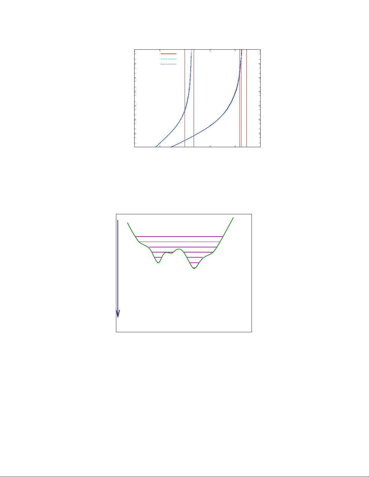
1 Constrain t optimisation and landscap es. Floren t Krzak ala 1 and Jorge Kurc han 2 , (1) PCT-ESPCI CNRS UMR Gulliv er 7083 and (2) PMMH-ESPCI, CNRS UMR 7636, 10 rue V auquelin, 75005 P aris, FRANCE W e describ e an effectiv e landscap e in tro duced in [1] for the analysis of Constrain t Sat- isfaction problems, such as Sphere P ac king, K-SA T and Graph Coloring. This geometric construction reexpresses these problems in the more fa miliar terms of optimisation in ru gged energy landscapes. In particular, it allo ws one to underst and the puzzling fact that unsophis- ticated programs are successful w ell b eyon d what w as considered to b e the ‘hard’ transition, and suggests an algorithm defining a new, higher, easy-hard frontier. P A CS Num b ers : 75.10.Nr, 02.50.-r,64.70.Pf, 81.05.Rm 2 Amongst glassy systems, the particular class of ‘Constrain t Optimisation’ has received constan t atten tion [2, 3]. These are problems in which we are given a set of constrain ts that m ust be satisfied, and our task is to optimize the conditions without violating them. The t ypical example is pac king: w e are ask ed to put as man y ob jects (spheres, sa y) in a given v olume, without violating the constrain t that they should not ov erlap. Another example that has b een widely studied by computer scien tists is K-SA T, where w e hav e N Bo olean v ariables, and αN logic clauses: our task is to add more and more clauses while still finding some set of v ariables that satisfy them. One last example is the q -coloring problem: w e ha v e a graph with N nodes and αN links and our task is to color each vertex with one of q colours, with the condition that link ed v ertices ha v e differen t colours. If we consider a sequence of graphs as a set of no des and a predefined list of links, then adding links one by one mak es the problem harder and harder. What motiv ated our interest in these problems was what w e p ercieved as a confusing situation in the literature. Consider first sphere packing. In Fig. 1 we sho w differen t v olume fractions that are often quoted in the literature. In particular ‘Random Close P ac king’ (as defined empirically) , the ‘ optimal random pac king’ (zero-temperature glass state) an d the so- called ‘J-p oin t’, are sometimes used as synon yms and sometimes not. The ’J-p oin t’ deserves random loose packing mode−coupling random close packing crystal J−point procedure Ideal glass state?? φ FIG. 1: The v arious transition densities for the sphere-pac king problem. some explanation. It can b e defined as follo ws [4]: one starts from small spheres in random p ositions, and ‘inflates’ them gradually (in the computer, of course), only displacing them the 3 least neccessary to av oid ov erlaps [6]. A t some p oin t the system blocks and the pro cedure stops: this is the J-p oint. It w as studied extensiv ely by the Chicago group [4, 5], who prop osed that it b e identified with Random Close Pac king. On the other hand, Random Close Pac king is often asso ciated with the zero-temperature ideal glass state. The tw o iden tifications seem hardly compatible, as they would imply that the fast algorithm describ ed ab o ve allows to find rapidly the ideal glass state, con trary to all our prejudices. Let us now turn to the SA T and Colouring problems. Carrying o ver the kno wledge from mean-field glasses, it was concluded that the set of solutions evolv es, as the difficult y is increased, in the following manner: for low α the set of solutions is connected. As α is increased there is a well defined ‘dynamic’ or ‘clustering’ p oin t α d at which the set of satisfied solutions breaks into man y comparable disconnected pieces [11]. A t a larger v alue α K the volume b ecomes dominated b y a few regions, and finally , at some α c , there are no more solutions [7]. Bey ond the clustering transition α d the problem was thought to b ecome har d . And yet, as it turne d out, even very simple pr o gr ams[15] manage to find solutions wel l b eyond this har d tr ansition! The situation is show ed in Fig. 2. This is another puzzle we set out to clarify . A first observ ation one can mak e is that the ‘J-p oin t’ pro cedure can b e generalised to all of these problems: one just has in all cases to increase the difficulty gradually , and keep the system satisfied b y minimal changes each time. F or example, for the Colouring problem, one adds one link at a time, and corrects any miscoloring generated by suc h an addition. The n um b er of colour flips needed each time to correct the miscoloring gro ws and it div erges with a well -defined, repro ducible p o w er la w (see Fig. 3) at a v alue α ∗ , by definition the limit reac hed b y the program. Second, and most imp ortan t, w e in tro duce a (pseudo) energy landscap e as follows (see Fig. 4). As the difficulty in the problem is increased – by increasing the radius, or adding clauses, or adding links – the set of satisfied configurations b ecomes a subset of the previous one. This allo ws to construct a single-v alued env elop e function (Fig. 4): the pseudo-energy . It is e asy to se e that the J-p oint pr o c e dur e is just a zer o-temp er atur e desc ent on this landsc ap e . W e can now carry ov er everything we kno w from energy landscap es. F or the J-point in the con text of sphere pac kings, w e conclude that: 4 α d α sp α α d α α sp α α asat c 3 − SAT c 3 − COLORING (3.86 , 4.21 , 4.245 , 4.267) (2.0 , 2.275, 2.3 , 2.345) * FIG. 2: Why is it so easy to go b eyond α d , the putativ e ‘har d’ limit? V alues of the parameter: i) α d the ‘clustering’ transition, ii) α AS AT for ASA T, α ∗ for our algorithm, iii) α S P the p erformance of a Survey Propagation implemen tation, and iv) α c the optimum [8]. • The J-p oin t, b eing the result of a gradient from a random configuration, cannot b e the optimal amourphous solution. It is just the analogue of the infinite temp er atur e inher ent structur es. • It is in general more co mpact than the clustering (Mode Coupling) poin t, since it gains from ‘falling to the b ottom of one cluster’. • It may b e more or less compact than the Kauzmann ( α K ) p oin t itself, depending on the dimension, p olydispersity , shap e, etc. F or problems suc h as SA T and Coloring, we ha ve no w a r e cursive incr emental algorithm, in which one increases the difficulty at small steps, at the same time correcting the configu- ration minimally in order to sta y satisfied [12]. This algorithm finds solutions in p olynomial time up to a α ∗ ≥ α d . Once α d is reached, the current solution remains ‘trapp ed’ within one cluster. On increasing further α (for example, in the Coloring problem, b y adding further links), the cluster of solution contracts un til it finally dissapp ears at α ∗ . As one can see in Fig. 2, one can go quite a long wa y b ey ond α d . How m uch so dep ends on ho w fast the cluster dissap ears: gradually for small q and K (in Coloring and SA T, resp ectiv ely), and 5 1 10 100 1000 10000 100000 1e+06 1e+07 0 1 2 3 4 5 time/N α q=3 q=4 α d = α K α uncol α d α K α uncol N=10 5 N=2.10 5 N=4.10 5 FIG. 3: In tegrated n umber of colour flips needed to av oid miscolourings, p er unit size, for the three and four colouring problem. The clustering transition and glass transitions are no obstacle. radius number of clauses, number of links, ... FIG. 4: Pseudo-energy (conjugated to pressure) landscape for constraint optimisation problems. The sets of satisfied configurations at increasing levels of difficult y are included in the previous: this allows for the definition of a w ell-defined en vel op e. essen tially immediately for large q , K and for problems that ha v e v ariables whose v alue is frozen within a cluster. Our conjecture is that unsophisticated programs will not do b etter than α ∗ , or rather, 6 than its ‘sl ow annealing’ v ersion as abov e [12]. Comparison with message-passing algorithms suc h as Belief and Surv ey Propagation is complicated by the fact that neither our v ersion of the Recursiv e Incremental program, nor the published implemen tations of Survey Prop- agation hav e b een pushed to their optimu m [13]. With this ca veat, the Surv ey Propagation algorithm seems to do b etter in the Coloring problem. On the other hand, Braunstein and Zecc hina ha ve recently shown that a message-passing algorithm do es well in the Binary P erceptron model [14] – a problem with single-configuration states – and this suggests that these algorithms go b ey ond α ∗ in that case. At any rate, it would b e v ery in teresting to explore along these lines the K = 3 SA T problem, a muc h b etter studied case. P erhaps the greatest promise of this approach comes from the fact that, as w e hav e indicated in Ref. [1], α ∗ defined b y the Recursive Incremental algorithm lends itself, due to its simple geometric definition, to an analytic computation. [1] F. Krzak ala and J. Kurchan, Phys. Rev. E 76 , 021122 (2007) [2] G. Parisi, Lectures of the V arenna summer sc ho ol, arXiv:cs/0312011. [3] M. Garey and D. S. Johnson, Computers and Intr actability: a Guide to the the ory and NP- c ompleteness (F reeman, San F rancisco, 1979); C.H. P apadimitriou, Computational Complexity (Addison-W esley , 1994). [4] C. S. O’Hern, L. E. Silb ert, A. J. Liu, S. R. Nagel, Phys. Rev. E 68 , 011306 (2003) [5] See also M. Wy art, Annales de Ph ysique, V ol. 30 No. 3 (2005). [6] An infinitely fast version of: B. D. Lubac hevsky and F. H. Stillinger, J. Stat. Phys. 60 , 561 (1990). [7] See, for a recent discussion: F. Krzak ala, A. Montanari, F. Ricci-T ersenghi, G. Semerjian and L. Zdeb oro v´ a, cond-mat/0612365. Pro c. Natl. Acad. Sci. 104, 10318 (2007). [8] F or the 3-SA T problem transition p oin ts see A. Montanari, G. P arisi, F. Ricci-T ersenghi J. Ph ys. A 37 , 2073 (2004), and refs [7, 9]. The v alue of α W S is a v ariant of W alk SA T, see: John Ardelius and Erik Aurell, Phys. Rev. E 74, 037702 (2006). F or a Survey Propagation implemen tation for the SA T problem see Ref. [9] and J Chav as, C F urtlehner, M Mezard and R Zecchina, J. Stat. Mech. (2005) P11016 F or the 3-coloring transition p oin ts see: L. Zdeb oro v´ a and F. Krzak ala, Phase tr ansitions in 7 the c oloring of r andom gr aphs , arXiv:0704.1269v1 (2007). The v alue of α ∗ is the one obtained b y the algorithm describ ed here (see Ref. [1]). The v alue for a survey propagation program is tak en from [10]. [9] M´ ezard M, Zecchin a R, Phys. Rev. E 66 056126 (2002); M ´ ezard M, P arisi G, Zecch ina R, SCIENCE 297 812 (2002) [10] Mulet R, P agnani A, W eigt M, et al. , Ph ys. Rev. Lett. 89 268701 (2002) [11] The clustering p oin t is the Mo de-Coupling transition p oint of glass theory , recently extended to dilute systems in: A Mon tanari, G Semerjian, J. Stat. Phys. 125 , 23 (2006). [12] One can also env isage a further impro v ement , in analogy with the Lubachevsky-Stillinger [6] algorithm: one can follo w each increase in α with a num b er of steps of diffusion b et w een satisfied solutions. [13] Our program is not optimal b ecause we used a W alk-Col routine to find the finite n umber of recolorings at each step. An exhaustiv e enumeration would ha ve found the minimal num b er of recolorings, and this may div erge at a larger v alue of α , thus yielding a larger v alue of α ∗ . On the other hand, the Surv ey Propagation routines ha ve a large freedom in the metho d of going from fields to configurations, and this has not b een fully exploited y et. [14] Braunstein A, Zecchina R, Phys. Rev. Lett. 96 030201 (2006) [15] Here by ‘simple’ or ‘unsophisticated’ we mean ‘using no sp ecific knowledge of the glass state’.