Quantization of Prior Probabilities for Hypothesis Testing

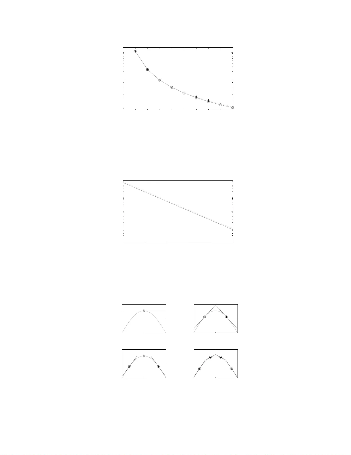
1 Quantizati on of Pri or Probabil ities for Hypothesis T esting Kush R. V arshney and Lav R. V arshney Abstract Bayesian hypothesis testing is investigated when the prior p robabilities o f the hy potheses, taken as a rando m vector , are quantized. Nearest neighbor and centroid conditions are deri ved using mean B ayes risk error as a distortion measure for qua ntization. A high-r esolution approximation to the distortio n-rate function is also ob tained. Human decision making in segregated population s is studied assuming Bayesian hyp othesis testing with quan tized priors. Index T erms quantization , cate gorization, Bayesian hypo thesis testing, detection, classification, Bayes r isk error I . I N T RO D U C T I O N C ONSIDER a hypothes is te sting sc enario in which an ob ject is to b e ob served to d etermine whic h on e of M states, { h 0 , . . . , h M − 1 } , it is in. T he objec t has prior probability p m of being in state h m , i.e. p m = Pr[ H = h m ] , and prior probability vector p =  p 0 · · · p M − 1  T , with P M − 1 m =0 p m = 1 , which is known to the dec ision maker . M -ary hypothes is testing with known prior probab ilities calls for the Bayesian formulation to the problem, for which the optimal de cision rule minimizes Bayes risk [2]. Now consider the situation whe n there is a p opulation of ob jects, eac h with its own prior probability vector drawn from the distrib ution f P ( p ) supp orted on the ( M − 1) -dimensional proba bility simplex. If the prior probab ility vector of each object were known perfectly to the decision maker before observation a nd hypo thesis testing, then the sce nario would b e no different than that of standard Bay esian hypothes is testing. Howev er , we cons ider the case in which the decision maker is constrained an d ca n o nly work with a t mo st K dif ferent p rior proba bility vectors. Such a cons traint is moti v ated by scena rios whe re the decision ma ker has finite memo ry or limited information process ing resource s. He nce, wh en there are more tha n K ob jects in the population, the d ecision ma ker must first map the true p rior prob ability vector of the object being o bserved to one of the K av ailable vectors and then proceed to perform the o ptimal Bayesian hypo thesis test, treating that vector as the prior proba bilities of the object. Although no t the only su ch constrained scenario, one exa mple is tha t of h uman decis ion making. On e particular setting is a referee deciding whe ther a player has committed a foul us ing his or her noisy obse rvati on as we ll as prior experience. Play ers commit fouls at different rates ; s ome players are dirtier or more ag gressive than othe rs. It is this rate which is the prior probability for the ‘foul committed’ state. Hen ce, over the p opulation o f p layers, there is a distribution of p rior p robabilities. If the referee tune s the prior probab ility to the particular player on whose action the decision is to be ma de, de cision-making performance is improv ed. Human d ecision ma kers, howe ver , are limited in their information process ing capac ity and c an on ly carry around seven, plus or minus two, categories withou t getting con fused [3]. Consequently , the referee is li mited and categorizes players into a sma ll number o f dirtiness levels, with assoc iated representative p rior proba bilities, exactly the sc enario described above. In this pa per , the des ign of the mapping from prior p robability vectors in the population to one of K representative probability vectors is approa ched as a quantization p roblem. Mean Ba yes risk e rror (MBRE) is define d as a fidelity criterion for the qu antization of f P ( p ) and conditions are derived for a minimum MBRE quantize r . Some examples K. R . V arshney and L. R. V arshney are wi th the Laboratory for Information and Decision Systems, Massachusetts Insti tute of T echnology , Cambridge, MA 02139 US A (e-mail: krv@mit. edu; lrv@mit.edu). Part of the material i n this paper was presented at the 2008 IEEE International Conference on Acoustics, S peech, and Signal Processing [1]. This work was supported in part by NSF Graduate Research Fellowships to K. R. V arshne y and L. R. V arshney . 2 of MBRE-op timal qua ntizers are giv en alon g with the ir p erformance in the low- rate q uantization regime. Distortion- rate functions are g i ven for the high-rate quantization regime. Certain human decision-mak ing tasks , as mentioned above, may be mod eled by quantized prior hypothe sis testing d ue to certain subo ptimalities in human information process ing. Hu man dec ision making is ana lyzed in detail for segregated po pulations, rev ealing a ma thematical model of s ocial discrimination. Previous work that comb ines d etection and quantization look s at the quantization of obs erved data, not prior probabilities, and also only approximates the Ba yes risk fun ction instead of working with it directly , e. g. [4]–[6] and referen ces cited in [6]. In s uch work, there is a co mmunication cons traint between the sensor and the decision maker , but the decision maker has unco nstrained proce ssing capability . Our work de als with the opposite cas e, where there is no c ommunication constraint betwe en the sen sor and the d ecision maker , howe ver the dec ision maker is co nstrained. A brief loo k a t imperfect priors a ppears in [7, Sec. 2.E], but optimal quantization is not considered . In [8], [9], it is s hown that small deviations from the true prior yield small deviations in the Bayes risk. W e are not aware of any p revi ous work that has looked at quantization, clustering, o r categorization of prior probabilities. In the remainder of the paper , we foc us on binary h ypothesis testing, M = 2 . Section II define s the Baye s risk error dis tortion an d giv es some o f its properties. Sec tion III discus ses lo w-rate quantiza tion and S ection IV discuss es high-rate qua ntization. Some examp les with a Gauss ian mea surement model a re given in Section V. Section VI considers the implications o n h uman decis ion making a nd Section VII provides a summa ry a nd d irections for future work. I I . B A Y E S R I S K E R RO R In the b inary Bay esian hy pothesis testing problem for a given o bject, the re are two hypotheses h 0 and h 1 with prior proba bilities p 0 = Pr[ H = h 0 ] an d p 1 = Pr[ H = h 1 ] = 1 − p 0 , a n oisy obse rv ation Y , a nd likelihoods f Y | H ( y | h 0 ) and f Y | H ( y | h 1 ) . Note tha t we c onsider a one-shot measu rement Y , rather than a s et of ind epende nt, noisy me asurements. A function ˆ h ( y ) is des igned that uniquely maps every possible y to either h 0 or h 1 in s uch a way that the function is optimal with respect to Bayes risk J = E [ c ( H i , H j )] , an expe ctation over the non-negative cost function c ( h i , h j ) . This g i ves the following specifica tion for ˆ h ( y ) : ˆ h ( · ) = arg min f ( · ) E [ c ( H, f ( Y ))] , (1) where the expe ctation is over bo th H and Y . It may b e shown that the optimal de cision rule ˆ h ( y ) is the likelihood ratio test: f Y | H ( y | h 1 ) f Y | H ( y | h 0 ) ˆ h ( y )= h 1 ⋚ ˆ h ( y )= h 0 p 0 ( c 10 − c 00 ) (1 − p 0 )( c 01 − c 11 ) , (2) where c ij = c ( h i , h j ) . There are two types of errors, with the follo wing proba bilities: p I E = Pr[ ˆ h ( Y ) = h 1 | H = h 0 ] , p II E = Pr[ ˆ h ( Y ) = h 0 | H = h 1 ] . Bayes risk may be express ed in terms of those error prob abilities as: J = ( c 10 − c 00 ) p 0 p I E + ( c 01 − c 11 )(1 − p 0 ) p II E + c 00 p 0 + c 11 (1 − p 0 ) . (3) It is often of interest to ass ign no c ost to c orrect decisions , i.e. c 00 = c 11 = 0 , wh ich we as sume in the remainder of this paper . In this case , the Bayes risk s implifies to: J ( p 0 ) = c 10 p 0 p I E ( p 0 ) + c 01 (1 − p 0 ) p II E ( p 0 ) . (4) In ( 4), the depend ence o f the Bayes risk and error probabilities on p 0 has been explicitly no ted. The error probabilities depend o n p 0 through ˆ h ( · ) , given in (2). T he function J ( p 0 ) is zero at the po ints p 0 = 0 and p 0 = 1 and is po siti ve- valued, strictly concave, and con tinuous in the interval (0 , 1) [2], [10], [11]. 3 In the case wh en the true prior probab ility is p 0 , b ut ˆ h ( y ) is des igned ac cording to (2) using some o ther v alue a sub stituted for p 0 , there is mismatch , and the mismatched Bayes risk is: ˜ J ( p 0 , a ) = c 10 p 0 p I E ( a ) + c 01 (1 − p 0 ) p II E ( a ) . (5) ˜ J ( p 0 , a ) is a linea r function of p 0 with slope ( c 10 p I E ( a ) − c 01 p II E ( a )) and intercept c 01 p II E ( a ) . Note that ˜ J ( p 0 , a ) is tangent to J ( p 0 ) at a and tha t ˜ J ( p 0 , p 0 ) = J ( p 0 ) . Definition 1 : Let Bayes risk error d ( p 0 , a ) be the diff erence between the mismatched Bay es risk function ˜ J ( p 0 , a ) and the Ba yes risk fun ction J ( p 0 ) : d ( p 0 , a ) = ˜ J ( p 0 , a ) − J ( p 0 ) = c 10 p 0 p I E ( a ) + c 01 (1 − p 0 ) p II E ( a ) − c 10 p 0 p I E ( p 0 ) − c 01 (1 − p 0 ) p II E ( p 0 ) . (6) W e now giv e properties of d ( p 0 , a ) a s a function of p 0 and as a function of a . Theorem 1: The Bay es risk error d ( p 0 , a ) is non -negati ve a nd only equa l to z ero when p 0 = a . As a function of p 0 ∈ (0 , 1) , it is c ontinuous and strictly con vex for all a . Pr oo f: Since J ( p 0 ) is a continuous a nd strictly concave function, a nd lines ˜ J ( p 0 , a ) are tange nt to J ( p 0 ) , ˜ J ( p 0 , a ) ≥ J ( p 0 ) for all p 0 and a , with equa lity whe n p 0 = a . Co nseque ntly , d ( p 0 , a ) is non-negative and only equal to zero when p 0 = a . Moreover , d ( p 0 , a ) is con tinuous a nd strictly c on vex in p 0 ∈ (0 , 1) for all a beca use it is the d if feren ce of a con tinuous linear function and a co ntinuous strictly concave function. Theorem 2: For any de terministic likelihood ratio test ˆ h ( · ) , as a func tion of a ∈ (0 , 1) for all p 0 , the Bay es risk error d ( p 0 , a ) h as exactly one s tationary point, which is a minimum. Pr oo f: Con sider the parameterize d curve ( p I E , p II E ) traced ou t as a is varied; this is a flippe d version of the receiv er op erating charac teristic (R OC). The flipped R OC is a strictly c on vex function for deterministic likelihood ratio tes ts. At its endpoints, it takes values ( p I E = 0 , p II E = 1) when a = 1 and ( p I E = 1 , p II E = 0) when a = 0 [2], and therefore has average s lope − 1 . By the mea n value theorem and s trict con vexity , there exists a un ique point on the flipped R OC a t which dp II E dp I E = − 1 . T o the left of that p oint: −∞ < dp II E dp I E < − 1 , a nd to the right of that po int: − 1 < dp II E dp I E < 0 . For deterministic likelihood ratio tests, β dp I E ( a ) da < 0 and γ dp II E ( a ) da > 0 for all a ∈ (0 , 1) and positi ve con stants β and γ [2]. Th erefore, if γ dp II E β dp I E < − 1 , i.e. γ dp II E da da β dp I E < − 1 , then γ dp II E da > − β dp I E da and β dp I E da + γ dp II E da > 0 . In the sa me manner , if γ dp II E β dp I E > − 1 , then β dp I E da + γ dp II E da < 0 . Combining the above, we find that the function β p I E ( a ) + γ p II E ( a ) has exactly on e stationa ry p oint in (0 , 1) , which oc curs whe n the slope of the flipped ROC is − β γ . De note this stationary point as a s . For 0 < a < a s , − 1 < dp II E dp I E < 0 a nd the slop e of β p I E ( a ) + γ p II E ( a ) is n egati ve; for a s < a < 1 , −∞ < dp II E dp I E < − 1 and the slope of β p I E ( a ) + γ p II E ( a ) is p ositi ve. Therefore, a s is a minimum. As a function of a , the Baye s risk e rror is of the form β p I E ( a ) + γ p II E ( a ) + C . H ence, it also has exac tly one stationary point a s , which is a minimum. As se en in Sec tion III, the above prope rties of d ( p 0 , a ) are useful to establish that the Lloyd-Max con ditions a re not on ly neces sary , but also sufficient for quantize r local optimality . The third deriv ative of d ( p 0 , a ) with respect to p 0 is: − c 10 p 0 d 3 p I E ( p 0 ) dp 3 0 − 3 c 10 d 2 p I E ( p 0 ) dp 2 0 − c 01 (1 − p 0 ) d 3 p II E ( p 0 ) dp 3 0 + 3 c 01 d 2 p II E ( p 0 ) dp 2 0 , (7) when the cons tituent deriv atives exist. As seen in Section IV, when the third deriv a ti ve exists and is c ontinuous, d ( p 0 , a ) is locally quadratic, which is useful to develop high-rate quantization theory for Ba yes risk error fidelity [12]. I I I . L O W - R A T E Q U A N T I Z A T I O N The conditions ne cessa ry for the optimality of a qu antizer for f P 0 ( p 0 ) under Ba yes risk error distortion are now deriv ed. A K -point quantizer partitions the interval [0 , 1] into K regions R 1 , R 2 , R 3 , . . . , R K . For eac h o f these quantization regions R k , there is a representation p oint a k to which eleme nts are mapped. For regular qu antizers, the regions are sub intervals R 1 = [0 , b 1 ] , R 2 = ( b 1 , b 2 ] , R 3 = ( b 2 , b 3 ] , . . . , R K = ( b K − 1 , 1] and the represen tation 4 p 0 J ( p 0 ) a k a k + 1 b k Fig. 1. The intersection of the lines ˜ J ( p 0 , a k ) , tangent to J ( p 0 ) at a k , and ˜ J ( p 0 , a k +1 ) , tangent to J ( p 0 ) at a k +1 , is the optimal interval boundary . points a k are in R k . 1 A quantizer ca n be viewed as a nonlinear function v K ( · ) such that v K ( p 0 ) = a k for p 0 ∈ R k . For a giv en K , we would like to find the qu antizer that minimizes the MBRE: D = E [ d ( P 0 , v K ( P 0 ))] = Z d ( p 0 , v K ( p 0 )) f P 0 ( p 0 ) dp 0 . (8) There is no closed-form solution, but an optimal quantizer must satisfy the nearest neighbor condition, the centroid condition, an d the ze ro proba bility of bound ary condition [13]. The ne arest neighb or and ce ntroid conditions are developed for MBRE in the follo wing sub sections. Whe n f P 0 ( p 0 ) is absolutely continuous , the zero probability of bounda ry co ndition is a lw ays satisfied. A. Near est N eighbor Cond ition W ith the representation p oints { a k } fixed , an expression for the interv al b oundaries { b k } is deri ved . Giv en any p 0 ∈ [ a k , a k +1 ] , if ˜ J ( p 0 , a k ) < ˜ J ( p 0 , a k +1 ) then Baye s risk error is minimized if p 0 is represe nted by a k , and if ˜ J ( p 0 , a k ) > ˜ J ( p 0 , a k +1 ) the n Ba yes risk error is minimized if p 0 is represented by a k +1 . The bounda ry point b k ∈ [ a k , a k +1 ] is the a bscissa o f the point at which the lines ˜ J ( p 0 , a k ) an d ˜ J ( p 0 , a k +1 ) intersec t. The idea is illustrated graphica lly in Fig. 1. By manipulating the slopes an d intercepts of ˜ J ( p 0 , a k ) an d ˜ J ( p 0 , a k +1 ) , the point of intersection is found to be: b k = c 01  p II E ( a k +1 ) − p II E ( a k )  c 01  p II E ( a k +1 ) − p II E ( a k )  − c 10  p I E ( a k +1 ) − p I E ( a k )  . (9) B. Centr oid Co ndition W ith the qu antization regions fixed, the MBRE is to be minimized over the { a k } . Here, the MBRE is expres sed as the sum of integrals over quantization regions: D = K X k =1 Z R k  ˜ J ( p 0 , a k ) − J ( p 0 )  f P 0 ( p 0 ) dp 0 . (10) Becaus e the regions a re fixed, the minimization may be performed for each interval s eparately . Let us define I I k = R R k p 0 f P 0 ( p 0 ) dp 0 and I II k = R R k (1 − p 0 ) f P 0 ( p 0 ) dp 0 , which are con ditional means. The n: a k = arg min a  c 10 I I k p I E ( a ) + c 01 I II k p II E ( a )  . (11) Since β p I E ( a ) + γ p II E ( a ) has exac tly one stationary point, which is a minimum (cf. Th eorem 2), equa tion (11) is uniquely minimized by setting its deri vati ve equal to zero. Thus, a k is the solution to: c 10 I I k dp I E ( a ) da    a k + c 01 I II k dp II E ( a ) da    a k = 0 . (12) 1 Due to the strict con ve xity of d ( p 0 , a ) in p 0 for all a shown in Theorem 1, quantizers that satisfy the necessary conditions for MBRE optimality are regular , see [13, Lemma 6.2.1]. Therefore, only regular quantizers are considered. 5 Commonly , dif feren tiation of the two error probabilities is tractable ; they are themselves integrals o f the likelihood functions an d the differentiati on is with respect to some function of the limits of integration. C. L loyd-Max Algor ithm Alternating b etween the neares t neighbor and centroid c onditions, the iterati ve Lloyd-Max algo rithm can be applied to find minimum MBRE quantizers [13]. The algorithm is wide ly used because of its simplicity , ef fec ti ven ess, and co n vergence prope rties [14]. In [15], it is shown tha t the conditions ne cessa ry for optimality of the quantizer are also s ufficient conditions for local op timality 2 if the follo wing hold. The first condition is that f P 0 ( p 0 ) must be positiv e and con tinuous in (0 , 1) . The secon d con dition is tha t R 1 0 d ( p 0 , a ) f P 0 ( p 0 ) dp 0 must be finite for a ll a . The first and sec ond cond itions are met b y co mmon distrib utions su ch as the beta distribution [16]. The third condition is that the d istortion function d ( p 0 , a ) must satisfy some prop erties. It mu st b e zero on ly for p 0 = a , continuo us in p 0 for a ll a , a nd conv ex in a ; the first two o f the se hold as discu ssed in Theorem 1. The third, con vexity in a , d oes n ot hold for Bayes risk error in g eneral, but the conv exity of d ( p 0 , a ) in a is on ly used by [15] to s how that a unique minimum exists. As shown in Theorem 2, d ( p 0 , a ) ha s a unique stationary point that is a minimum. Therefore, the analysis of [15] applies to Bay es risk error distortion. Th us, if f P 0 ( p 0 ) satisfies the first and second conditions, then the algorithm is guaranteed to con verge to a local optimum. The algorithm may be run many times with different initializations to find the global optimum. Further conditions on d ( p 0 , a ) and f P 0 ( p 0 ) a re given in [15 ] for there to be a unique locally op timal qu antizer , i.e. the glob al optimum. If these further co nditions for unique local optimality hold, the n the algorithm is g uaranteed to find the globally minimum MBRE qua ntizer . In many prac tical s ituations, the distrib ution f P 0 ( p 0 ) is not av a ilable, but d ata d rawn from it is available. The optimal design o f qua ntizers from data is NP-hard [17], [18]. Howe ver , the Lloyd-Max a lgorithm and its close cousin K -mea ns can be used on da ta with the Ba yes risk e rror fidelity criterion. In fact, a s the size of the da taset increases , the se quence of q uantizers de signed from data co n verges to the quantizer d esigned from f P 0 ( p 0 ) [19 ], [20]. (Conditions o n the distortion function given in [20 ] exce pt con vexity in a are met by the Bayes risk error , but in a similar way to the s uf ficiency of the Lloyd-Max conditions, the un ique minimum property of the Bay es risk error is enoug h.) D. Mo notonic Conver gence in K Let D ∗ ( K ) = P K k =1 R R ∗ k d ( p 0 , a ∗ k ) f P 0 ( p 0 ) dp 0 denote the MBRE for an optimal K -point quantizer . W e show that D ∗ ( K ) mo notonically c on verges as K increase s. The MBRE-optimal K -point quantizer is the solution to the follo wing problem: minimize K X k =1 Z b k b k − 1 d ( p 0 , a k ) f P 0 ( p 0 ) dp 0 such that b 0 = 0 b K = 1 b k − 1 ≤ a k , k = 1 , . . . , K a k ≤ b k , k = 1 , . . . , K. (13) Let us add the additional c onstraint b K − 1 = 1 to (13 ), forcing a K = 1 and degene racy of the K th quantization region. The optimization problem for the K -point quan tizer (13) with the additional cons traint is equiv alent to the optimization proble m for the ( K − 1 )-point qu antizer . Thus, the ( K − 1 )-point design prob lem and the K -point des ign problem h av e the same obje cti ve function, but the ( K − 1 )-point prob lem ha s a n ad ditional con straint. The refore, D ∗ ( K − 1) ≥ D ∗ ( K ) . Since d ( p 0 , v K ( p 0 )) ≥ 0 , D = E [ d ( P 0 , v K ( P 0 ))] ≥ 0 . Since the s equenc e D ∗ ( K ) is no nincreasing a nd bound ed from b elow , it conv er ges. Mean Bayes risk error cannot g et worse whe n more quan tization lev els are employed. 2 By local optimalit y , it is meant that the { a k } and { b k } minimize t he objecti ve function (8) among feasible representation and boundary points near t hem. 6 In typical s ettings, as in Section V, performanc e always improves with an increase in the number o f qu antization lev els. I V . H I G H - R A T E Q UA N T I Z AT I O N Let us ap ply high-rate quantization theory [14] to the study of minimum MBRE quantization. The distortion function for the MBRE criterion has a positiv e s econd de ri vativ e in p 0 (due to strict con vexity) and for many famili es of likelihood func tions, it has a continuous third deriv a ti ve, s ee (7). Thus, it is loca lly qu adratic in the sense of Li et al. [12] and in a man ner similar to many p erceptual, non-difference distortion func tions, the high-rate quantization theory is well-developed. At h igh rate, i.e . K large, if we let: B ( p 0 ) = − 1 2 c 10 p 0 d 2 p I E ( p 0 ) dp 2 0 − c 10 dp I E ( p 0 ) dp 0 − 1 2 c 01 (1 − p 0 ) d 2 p II E ( p 0 ) dp 2 0 + c 01 dp II E ( p 0 ) dp 0 , (14) then d ( p 0 , a k ) is approximated by the follo wing sec ond order T ay lor expansion : d ( p 0 , a k ) ≈ B ( p 0 ) | p 0 = a k ( p 0 − a k ) 2 , p 0 ∈ R k . (15) Assuming that f P 0 ( · ) is s ufficiently smooth and subs tituting (15) into the o bjectiv e of (13), the MBRE is approxi- mated by: D ≈ K X k =1 f P 0 ( a k ) B ( a k ) Z R k ( p 0 − a k ) 2 dp 0 . (16) The MBRE is greater than an d approximately equal to the followi ng lo wer bound , deri ved in [12] by relationships in volving normalized momen ts of inertia of intervals R k and by H ¨ older’ s inequality: D L = 1 12 K 2 Z 1 0 B ( p 0 ) f P 0 ( p 0 ) λ ( p 0 ) − 2 dp 0 , (17) where the optimal qua ntizer po int dens ity is: λ ( p 0 ) = ( B ( p 0 ) f P 0 ( p 0 )) 1 / 3 R 1 0 ( B ( p 0 ) f P 0 ( p 0 )) 1 / 3 dp 0 . (18) Integrating a quantizer point dens ity over an interval yields the fraction of the { a k } that are in tha t interval. Substituting (18) into (17) y ields: D L = 1 12 K 2 k B ( p 0 ) f P 0 ( p 0 ) k 1 / 3 . (19) V . E X A M P L E S As a n example, let us consider the following sca lar signal and measurement model: Y = s m + W, m ∈ { 0 , 1 } , (20) where s 0 = 0 and s 1 = µ (a known, deterministic qu antity), and W is a zero-mean, Gaussian ran dom v ariable with variance σ 2 . The likelihoods a re: f Y | H ( y | h 0 ) = N ( y ; 0 , σ 2 ) = 1 σ √ 2 π e − y 2 / 2 σ 2 , f Y | H ( y | h 1 ) = N ( y ; µ, σ 2 ) = 1 σ √ 2 π e − ( y − µ ) 2 / 2 σ 2 . (21) The two error probabilities are: p I E ( p 0 ) = Q  µ 2 σ + σ µ ln  c 10 p 0 c 01 (1 − p 0 )  , p II E ( p 0 ) = Q  µ 2 σ − σ µ ln  c 10 p 0 c 01 (1 − p 0 )  , (22) where: Q ( α ) = 1 √ 2 π Z ∞ α e − x 2 / 2 dx. 7 Finding the centroid cond ition, the de ri vativ e s of the error p robabilities are: dp I E ( p 0 ) dp 0    a k = − 1 √ 2 π σ µ 1 a k (1 − a k ) e − 1 2 “ µ 2 σ + σ µ ln “ c 10 a k c 01 (1 − a k ) ”” 2 , (23) dp II E ( p 0 ) dp 0    a k = + 1 √ 2 π σ µ 1 a k (1 − a k ) e − 1 2 “ µ 2 σ − σ µ ln “ c 10 a k c 01 (1 − a k ) ”” 2 . (24) By substituting these deri vati ves into (12) and simpli fying, the follo wing expres sion is o btained for the representation points: a k = I I k I I k + I II k . (25) For high-rate ana lysis, the se cond deriv a ti ves of the error proba bilities are nee ded. They are: d 2 p I E ( p 0 ) dp 2 0 = − 1 √ 8 π σ µ 1 p 2 0 (1 − p 0 ) 2 e − 1 8 µ 2 σ 2 “ µ 2 +2 σ 2 ln “ c 10 p 0 c 01 (1 − p 0 ) ”” 2 h − 3 + 4 p 0 − 2 σ 2 µ 2 ln  c 10 p 0 c 01 (1 − p 0 ) i , (26) and: d 2 p II E ( p 0 ) dp 2 0 = + 1 √ 8 π σ µ 1 p 2 0 (1 − p 0 ) 2 e − 1 8 µ 2 σ 2 “ µ 2 − 2 σ 2 ln “ c 10 p 0 c 01 (1 − p 0 ) ”” 2 h − 1 + 4 p 0 − 2 σ 2 µ 2 ln  c 10 p 0 c 01 (1 − p 0 ) i . (27) By inspection, we note that the third de ri vativ es are continuou s. Sub stituting the first deriv a ti ves (23)-(24) and second de ri v ati ves (26)-(27) into (14), an expression for B ( p 0 ) can be obtained. Examples with diff erent dis trib u tions f P 0 ( p 0 ) are p resented below . All of the examples use sc alar signals with additiv e Gau ssian noise, µ = 1 , σ = 1 (20). As a point of referenc e, a comparison is ma de to qua ntizers designed under mean abso lute error (MAE) [21], i.e. d ( p 0 , a ) = | p 0 − a | , an objec ti ve tha t d oes no t a ccount for hypothe sis testing. 3 In the high-rate co mparisons, the op timal point dens ity for MAE [23 ]: λ ( p 0 ) = f P 0 ( p 0 ) 1 / 2 R 1 0 f P 0 ( p 0 ) 1 / 2 dp 0 is substituted into the high-rate distortion app roximation for the MBRE c riterion (17) . T aking R = log 2 ( K ) , there is a cons tant gap be tween the rates using the MBRE po int dens ity and the MAE point density for all dis tortion values. Th is dif ference is: R MBRE ( D L ) − R MAE ( D L ) = 1 2 log 2 k f P 0 ( p 0 ) B ( p 0 ) k 1 / 3 k f P 0 ( p 0 ) k 1 / 2 R 1 0 B ( p 0 ) dp 0 ! . The clos er the ratio inside the logarithm is to on e, the clos er the MBRE- and MAE-optimal q uantizers. A. Uniformly Distributed P 0 W e first look at the setting in which a ll prior proba bilities are equally likely . The MBRE of the MBRE-optimal quantizer and a quan tizer d esigned to minimize MAE with re spect to f P 0 ( p 0 ) are plotted in Fig. 2. (The optimal MAE qua ntizer for the uniform d istrib u tion is the uniform quantizer .) The plot sh ows MBRE as a fun ction of K ; the solid line with circle ma rkers is the MBRE-optimal quan tizer and the dotted line with asterisk markers is the MAE-optimal quan tizer . D L , the high-rate approximation to the d istortion-rate function is plotted in Fig. 3. The performanc e of both qu antizers is similar , but the MBRE-optimal qua ntizer always performs better or eq ually . For K = 1 , 2 , the two quantize rs a re iden tical, as seen in Fig. 4a-b . The plots in F ig. 4 show ˜ J ( p 0 , v K ( p 0 )) as solid and d otted lines for the MBRE- and MAE-op timal q uantizers resp ectiv ely; the markers are the represen tation points. The gray line is J ( p 0 ) , the Bayes risk with unqua ntized prior probabilities. For K = 3 , 4 , the repres entation points for the MBRE-optimal qu antizer are closer to p 0 = 1 2 than the uniform q uantizer . This is be cause the area under the po int dens ity function λ ( p 0 ) shown in F ig. 5 is concentrated in the center . Ea ch incremen t of K is as sociated 3 As sh o wn by Kassa m [21], minimizing the MAE criterion also minimizes the ab solute distance b etween the cu mulativ e distribution fun ction of the source and the induced cumulative distribution function of the quantized output. S ince the induced distribution from quantization is used as the population prior distribution for hypothesis testing, requiring this induced distribution to be close to the true unquantized distribution is reasonable. If distance between probability distributions i s to be mi nimized according t o the Kullback -Leibler discrimination between the true and induced distributions (which is defined in terms of l ikelihoo d ratios), an application of Pinsker’ s inequality sho ws that a small absolute difference is requisite [22]. Although a reasonable criterion, MAE is suboptimal for hypoth esis testing performance as seen in t he examp les. 8 0 1 2 3 4 5 6 7 8 9 10 −3 10 −2 10 −1 K D Fig. 2. MBRE for uniformly distributed P 0 and Bayes costs c 10 = c 01 = 1 plotted on a logarithmic scale as a function of the number of quantization levels K ; the solid l ine with cir cle markers is the MBRE-optimal quantizer and the dotted line with asterisk markers is the MAE-optimal uniform quantizer . 0 1 2 3 4 5 10 −5 10 −4 10 −3 10 −2 10 −1 D R (bits) Fig. 3. High-rate approximation of distortion-rate function D L for uniformly distributed P 0 and B ayes costs c 10 = c 01 = 1 ; the solid line is the MBRE-optimal quantizer and the dotted line is the MAE-optimal uniform quantizer . 0 0.5 1 0 0.2 0.4 p 0 ˜ J ( p 0 , v ( p 0 )) 0 0.5 1 0 0.2 0.4 p 0 ˜ J ( p 0 , v ( p 0 )) (a) (b) 0 0.5 1 0 0.2 0.4 p 0 ˜ J ( p 0 , v ( p 0 )) 0 0.5 1 0 0.2 0.4 p 0 ˜ J ( p 0 , v ( p 0 )) (c) (d) Fig. 4. Quantizers f or uniformly distributed P 0 and Bayes costs c 10 = c 01 = 1 . ˜ J ( p 0 , v K ( p 0 )) is plotted for (a) K = 1 , (b) K = 2 , (c) K = 3 , and (d) K = 4 ; the markers, circle and asterisk for the MBRE-optimal and MAE-optimal quantizers respectiv ely , are the representation points { a k } . The gray line is the unquan tized Bayes risk J ( p 0 ) . 9 0 0.2 0.4 0.6 0.8 1 0 0.2 0.4 0.6 0.8 1 1.2 1.4 p 0 λ ( p 0 ) Fig. 5. Opti mal MBRE point density for uniformly distributed P 0 and Bayes costs c 10 = c 01 = 1 . 0 1 2 3 4 5 6 7 8 9 10 −3 10 −2 10 −1 K D Fig. 6. MBRE for uniformly distributed P 0 and Bayes costs c 10 = 1 , c 01 = 4 plotted on a logarithmic scale as a function of the number of quantization levels K ; the solid l ine with cir cle markers is the MBRE-optimal quantizer and the dotted line with asterisk markers is the MAE-optimal uniform quantizer . with a lar g e red uction in Ba yes risk. There is a very large pe rformance improvement from K = 1 to K = 2 . In Fig. 6, Fig. 7, Fig. 8, and Fig. 9, similar plots to those ab ove are g i ven for the cas e when the Bayes co sts c 10 and c 01 are unequal. T he u nequal costs skew the Baye s risk fun ction and conseq uently the represen tation point locations and point dens ity function. The dif feren ce in pe rformance between the MBRE-optimal and MAE-optimal quantizers is greater in this example be cause the MAE-criterion cannot incorporate the Bayes costs, which factor into MBRE calculation. 0 1 2 3 4 5 10 −4 10 −3 10 −2 10 −1 10 0 D R (bits) Fig. 7. High-rate approximation of distortion-rate function D L for uniformly distributed P 0 and Bayes costs c 10 = 1 , c 01 = 4 ; the solid line is the MBRE-optimal quantizer and the dotted line is the MAE-optimal uniform quantizer . 10 0 0.5 1 0 0.5 1 p 0 ˜ J ( p 0 , v ( p 0 )) 0 0.5 1 0 0.5 1 p 0 ˜ J ( p 0 , v ( p 0 )) (a) (b) 0 0.5 1 0 0.5 1 p 0 ˜ J ( p 0 , v ( p 0 )) 0 0.5 1 0 0.5 1 p 0 ˜ J ( p 0 , v ( p 0 )) (c) (d) Fig. 8. Qu antizers for uniformly distributed P 0 and Bayes costs c 10 = 1 , c 01 = 4 . ˜ J ( p 0 , v K ( p 0 )) is plotted for (a) K = 1 , (b) K = 2 , (c) K = 3 , and (d) K = 4 ; the markers, circle and asterisk for the MBRE-optimal and MAE-optimal quantizers respectiv ely , are the representation points { a k } . The gray line is the unquan tized Bayes risk J ( p 0 ) . 0 0.2 0.4 0.6 0.8 1 0 0.5 1 1.5 2 2.5 p 0 λ ( p 0 ) Fig. 9. Opti mal MBRE point density for uniformly distributed P 0 and Bayes costs c 10 = 1 , c 01 = 4 . B. Beta Distributed P 0 Now , we look at a n on-uniform distrib ution for P 0 , in pa rticular the Beta( 5 , 2 ) d istrib ution. The proba bility density function is shown in Fig. 10. Th e MBRE o f the MBRE-optimal an d MAE-optimal qua ntizers are in Fig. 11. He re, there are also large improvements in pe rformance with an increase in K . The h igh-rate a pproximation to the distortion-rate function for this examp le is giv en in Fig. 1 2. The representation p oints { a k } are most densely distrib uted where λ ( p 0 ) , plott ed in Fig. 13, ha s mass. In p articular , more repres entation points are in the right half of the domain tha n in the left, a s see n in Fig. 14. 0 0.2 0.4 0.6 0.8 1 0 0.5 1 1.5 2 2.5 p 0 f P 0 ( p 0 ) Fig. 10. The probability density function f P 0 ( p 0 ) for the Beta( 5 , 2 ) distribution. 11 0 1 2 3 4 5 6 7 8 9 10 −3 10 −2 K D Fig. 11. MBRE for Beta( 5 , 2 ) distributed P 0 and Bayes costs c 10 = c 01 = 1 plotted on a l ogarithmic scale as a function of the number of quantization levels K ; the solid l ine with cir cle markers is the MBRE-optimal quantizer and the dotted line with asterisk markers is the MAE-optimal uniform quantizer . 0 1 2 3 4 5 10 −5 10 −4 10 −3 10 −2 10 −1 D R (bits) Fig. 12. High-rate approximation of distorti on-rate function D L for Beta( 5 , 2 ) distri buted P 0 and Bayes costs c 10 = c 01 = 1 ; the solid line is the MBRE-optimal quantizer and the dotted line is the MAE-optimal uniform quantizer . V I . I M P L I C A T I O N S O N H U M A N D E C I S I O N M A K I N G In the previous sections, we formulated the minimum MBRE quantiza tion problem and discusse d how to find the optimal MBRE quantizer . Having established the ma thematical foundations of hypothesis tes ting with q uantized priors, we ma y explore the implications of su ch resou rce-constrained d ecision mak ing o n hu man af fairs. Let us cons ider the p articular s etting for human de cision making mentioned in Section I : a referee determining whether a play er ha s committed a foul or not u sing both his or her noisy obse rv ation and p rior expe rience. The fraction of plays in which a playe r c ommits a foul is that playe r’ s prior proba bility for h 1 . Over the population of p layers, there is a distributi on of prior probabilities. Also as mentioned in Section I, huma n decision ma kers 0 0.2 0.4 0.6 0.8 1 0 0.5 1 1.5 2 p 0 λ ( p 0 ) Fig. 13. Optimal MBRE point density for Bet a( 5 , 2 ) distributed P 0 and Bayes costs c 10 = c 01 = 1 . 12 0 0.5 1 0 0.5 1 p 0 ˜ J ( p 0 , v ( p 0 )) 0 0.5 1 0 0.5 1 p 0 ˜ J ( p 0 , v ( p 0 )) (a) (b) 0 0.5 1 0 0.2 0.4 p 0 ˜ J ( p 0 , v ( p 0 )) 0 0.5 1 0 0.2 0.4 p 0 ˜ J ( p 0 , v ( p 0 )) (c) (d) Fig. 14. Quantizers for Beta( 5 , 2 ) distributed P 0 and Bayes costs c 10 = 1 , c 01 = 4 . ˜ J ( p 0 , v K ( p 0 )) i s plotted for (a) K = 1 , (b) K = 2 , (c) K = 3 , and (d) K = 4 ; the markers, circle and asterisk for the MBRE-optimal and MAE-optimal quantizers respectiv ely , are the representation points { a k } . The gray line is the unquan tized Bayes risk J ( p 0 ) . categorize into a small number of categories due to limitations in information proce ssing c apacity [3]. Decisions by humans may be modeled v ia quantization of the d istrib u tion of prior probabilities and the use of the quantization lev el c entroid of the ca tegory in which a player falls as the p rior probability when pe rforming hypothesis testing on that player’ s action. Therefore, a referee will do a be tter job with more ca tegories rather than fewer . A police officer co nfronting an indi vidual with who m he or she ha s p rior experienc e will make a b etter d ecision if he or s he has the mental categories ‘probably violent, ’ ‘possibly violent or nonvi olent, ’ and ‘prob ably n on violent, ’ versus just ‘violent’ an d ‘non violen t. ’ S imilarly , a do ctor will have a smaller prob ability of error when interpreting a blood test if he or she knows the prior probab ility of the test turning out p ositi ve for many c ategorizations of patients rathe r than jus t one for the entire pop ulation at lar ge. Additional examples c ould be gi ven for a variety of decision-making tasks . Implications of this so rt are not surprising. Howev er , when o ne additional compo nent is ad ded to the decision - making sce nario, some fairly interesting implications arise. Next, we look at the ca se when the quantization of two distinct pop ulations is don e separately . W e discuss mathe matically u nav o idable conse quenc es of quantize d prior h ypothesis testing when quantizing the prior probability for a minority population and the prior probability for a majority population sepa rately , while taking identical prior proba bility distributions of the two populations f P 0 ( p 0 ) . Although majority and minority pop ulations can b e defi ned along any soc ially observable dimension, such as gender o r age [24], for eas e of exp osition we use race, and more sp ecifically use ‘white’ an d ‘black ’ to den ote the two popula tions. Although there is s ome debate in the social cogn ition literature [25], it is thought that race and gender categorization is e ssentially automatic, particularly when a human a ctor lacks the moti vation, time, or co gniti ve cap acity to think d eeply . W e ca n extend the defi nition of MBRE to two popu lations as: D (2) = w w + b E [ ˜ J ( P 0 , v K w ( P 0 ))] + b w + b E [ ˜ J ( P 0 , v K b ( P 0 ))] − E [ J ( P 0 )] , (28) where w is the numbe r of wh ites encountere d, b is the number of black s e ncountered , 4 K w is the numbe r of p oints in the q uantizer for whites , and K b is the n umber of points in the qu antizer for blacks . In order to find the o ptimal allocation of the total quo ta of represe ntation points K t = K w + K b , we minimize D (2) for all K t − 1 possible allocations and choos e the best one; more soph isticated algorithms developed for b it allocation to subba nds in transform cod ing may also be used [27]. Fryer a nd J ackso n have pre viously s ugges ted that it is better to allocate more represen tation points to the majority population than to the minority popu lation [28]. W ith two se parate scalar quan tizers, but a single s ize constraint, 4 One might assume that w and b are simply the number of whites and blacks in the general population, howe ver these numbers should actually be based on the social i nteraction pattern of the decision maker . Due to seg regation in social interaction, see e.g. [26] and references therein, there is greater intra-population interaction than i nter-pop ulation i nteraction. The decision maker has more training data from intra- population interaction. 13 optimizing D (2) over v K w ( · ) an d v K b ( · ) yields the same res ult. Due to the monoton icity result in Se c. III-D, the MBRE for members of the minority group is greater than that for the majority g roup. Assuming white decision makers have w > b and black d ecision makers have b > w , an alysis of quantized prior Bayesian hy pothesis tes ting predicts that there should be own-race bias in decision mak ing. This prediction is in fact born out experimentally . A large body of literature in face recogn ition s hows exac tly the pred icted own race bias ef fect, observed c olloquially a s “ they [other-race persons] all look alike. ” In particular , both parts of the Bayes risk, p I E and p II E increase when trying to recogn ize members of the opp osite population [29]. V e rification of own race bias in face recog nition is due to labora tory experimentation, howev er similar ef fects have also been ob served in natural experiments through econ ometric s tudies. It has bee n fou nd that the addition of police of ficers of a giv en race is assoc iated with an increas e in the n umber of arrests o f sus pects o f a dif feren t race but has little impact on same-race arrests. Th e effect is more prono unced for minor offenses where the prior probab ility presumably plays a bigger role tha n the measureme nt [30]. The re are similar own-race bias effects in the decision by police to search a vehicle during a traffic stop [31], in the decision of h uman resource professionals to not hire [32], and in the decision of Na tional Basketball Asso ciation (NB A) referees to call a foul [33]. The rate of search ing, the rate of n ot hiring, and the rate of foul calling are all greater wh en the de cision-maker is of a dif ferent race than the d ri ver , applicant, an d player , respectively . A major dif ficulty in interpreting the se econ ometric studies, howe ver , is that the grou nd truth is not known. Highe r rates may be exp lained by either g reater p I E or smaller p II E . Since g round truth is lacking in econome tric s tudies, it is not clear how to interpret a finding tha t white referees call more fouls on black playe rs a nd that black referees call more fouls on white playe rs. Th is phenomen on canno t simply be explained b y a larger probab ility of d ecision error . The Bayes risk mus t be teased a part into its constituent parts and the Bayes c osts must be examined in detail. The meas urable quantity in an ec onometrics study is the probab ility that a foul is ca lled: Pr[ ˆ H K = h 1 ] = 1 − p 0 + p 0 p I E ( v K ( p 0 )) − (1 − p 0 ) p II E ( v K ( p 0 )) . (29) Looking at the average p erformance o f a white refere e over the popu lations of black an d white players, we co mpare the expe cted foul rates on whites and blac ks ( K b < K w ): ∆ = E h Pr[ ˆ H K b = h 1 ] − Pr [ ˆ H K w = h 1 ] i . (30) If this discrimination quantity ∆ is greater than zero, then the white referee is calling more fouls on blacks. If ∆ is less than zero, the n the referee is ca lling more fouls on whites. Th e ∆ expression may be written a s: ∆( c 10 , c 01 ) = E [ p 0 p I E ( v K b ( p 0 )) − (1 − p 0 ) p II E ( v K b ( p 0 ))] − E [ p 0 p I E ( v K w ( p 0 )) − (1 − p 0 ) p II E ( v K w ( p 0 ))] . (31) The de pende nce of ∆ on c 10 and c 01 is explicit on the left s ide of (31) a nd is implicit in the error probabilities on the right side . The value of ∆ also de pends on the unq uantized prior distributi on f P 0 ( p 0 ) , the me asurement model, and the q uantizer . If the prior d istrib u tion and measuremen t model are fixed, and the MBRE-optimal quantizer u sed, we find that the regions in the c 10 - c 01 plane whe re a wh ite referee would c all more fouls on b lacks and wh ere a white referee would call more fouls on whites are h alf-planes. For the uniform prior f P 0 ( p 0 ) , the dividing line between the two regions is exactly c 01 = c 10 . For the Beta( 5 , 2 ) prior , the dividing line is c 01 = mc 10 , whe re m > 1 . Using the di vision of the c 10 - c 01 plane into two parts, we c an now interpret the econome tric find ings in the NB A referee study [33] and related results [30]–[32 ]. The NB A race bias obse rvati ons can be gene rated from the quantized prior hy pothesis testing mode l o nly if the Baye s risk e rror has co sts c 01 > c 10 for a uniform p rior or costs c 01 ≫ c 10 for a Beta( 5 , 2 ) prior . The cho ice of B ayes c osts with c 01 greater tha n c 10 implies that a referee can tolerate more instances of calling fouls on play s that are n ot fouls rathe r than the oppos ite. This ass ignment of costs ha s been ca lled the p recautionary principle in some contexts. V e ry simply , the precautionary principle s tates “better safe tha n so rry . ” T aken together , the hypothesis testing with quantized priors model, the phenomenon of racial segregation [26], a nd results from econometric studies [30]–[33 ] sugge st that referees, police of ficers, a nd human resources professionals all follow the prec autionary principle. 14 V I I . C O N C L U S I O N A N D F U T U R E W O R K W e h av e looked at Ba yesian hyp othesis testing when there is a distribution of prior proba bilities, but the d ecision maker may on ly us e a quan tized version of the true prior probab ility in design ing a decision rule. Considering the problem o f finding the optimal quantizer for this purpos e, we have define d a new fidelity criterion bas ed on the Bayes risk function. For this c riterion, MBRE, we have determined the c onditions that an op timal quantizer satisfie s and worked through a high-rate approximation to the d istortion. M -ary hy pothesis tes ting with M > 2 requires vector quantiza tion rather than scalar q uantization, but d etermining the Lloyd-Max co nditions and high-rate theo ry is no different conceptually due to the ge ometry of the Bayes risk function a nd mismatched Bayes risk function. For the M -ary hypo thesis testing cas e, a multiv ariate distribution such a s the M -dimens ional Dirichlet distributi on [16] is n eeded for f P ( p ) . Previous, though sign ificantly different, work on quantization for hyp othesis testing was unable to d irectly minimize the Baye s risk, as was a ccomplished in this work. The mathema tical theory of qu antized prior h ypothesis testing formulated here leads to a ge nerativ e model of discriminati ve be havior when combined wit h theories of social c ognition and empirical facts about social segregation. This b iased de cision making arises de spite having iden tical distributions for different popu lations and despite no malicious intent on the part of the d ecision maker . W e a lso disc ussed how the choice of Bay es costs affects detection probabilities; in particular , the prec autionary principle leads to a higher detection p robability for the opposite ra ce, whereas a more op timistic view leads to a h igher detection probability for the own race. Such a phe nomenon of pess imistic or o ptimistic attitude fundame ntally a ltering the nature of disc rimination seems not to have be en described be fore. Dis crimination on the basis o f race, gen der , and othe r so cially ob servable cha racteristics has bee n a troublesome social problem, but appears to be a permane nt artifact of the automaticity of c lassification and the finite hu man capacity for information proces sing. There are many avenues along which to extend this work, suc h a s dealing with de centralized detection and classifica tion (with poss ible implications on jury d ecisions and elec tions), which ma y become game theoretic; consideration o f additional noise before or after quantization of the prior prob abilities; or the development of succe ssiv ely refin able q uantizers (for decision makers that poss ess a memory hierarchy). One can also c onsider a restricted class of quan tizers rather than conside ring optimal quan tization. Such restriction may mo del further cognitiv e co nstraints on human decision makers. In particular , Fryer an d Jacks on have su ggested a heuristic a lgorithm for quantizer design based on splitting group s [28], which is a rediscovery of the tree-structured vector quantizer (TSVQ) de sign algorithm g i ven in [34, F ig. 20 ]. Beyond [34], the re has been much recent d ev elopment in the theory of T SVQ pe rformance and recu rsi ve partitioning, which may prove useful. For the qua ntizer with K = 1 , an a lternati ve to the MBRE-optimal rep resentation po int: a ∗ MBRE = arg min a  Z ˜ J ( p , a ) f P ( p ) d p  is the min-max hypothe sis testing representation point: a ∗ min-max = arg min a  max p ˜ J ( p , a )  , which is only e quiv alen t in spec ial case s. A distribution on the prior probabilities is need ed to specify a ∗ MBRE , but n ot to spe cify a ∗ min-max . One ma y cons ider extending the min-max ide a to K > 1 . This would in volve an approach rela ted to  -entropy [35, Sec . 6 .1.2] and find ing a cover for the unit simplex by K sets of the form R k = { p | ˜ J ( p , a k ) ≤ D } , wh ere all p in R k map to a k and D is the sa me for all R k . The gen eral theme of ma chine learning for the explicit purpos e of hypo thesis testing, within which this work falls, is receiving increa sing attention; framing the hyp othesis tes ting scenario discus sed he re in terms of proba bilistic graphical models of c ategorization, e.g . the laten t Dirichlet alloca tion model [36 ] an d the h ierarchical Dirichlet process mixture model [37], ma y prove insightful as we ll. A C K N O W L E D G M E N T The authors than k V iv ek K Goyal, San joy K. Mitter , an d Alan S. W illsky , as well as the an onymous revie wers for valuable comments that led to improvement of the paper . 15 R E F E R E N C E S [1] K. R. V arshney and L. R. V arshney , “Minimum mean Bayes risk quantization of prior probabilities, ” in Pro c. IEEE Int. Conf. Acoustics, Speec h, Signal Pr ocessing , Las V egas, NV , Apr . 2008, pp. 3445–3448. [2] A. S. Willsky , G. W . W ornell, and J. H. Shapiro, Stoch astic Proce sses, Detection and Esti mation 6.432 Course Notes . Cambridge, MA: Dept. Elect. E ng. Comput. Sci. , Mass. Inst. T ech., Fall 2003. [3] G. A. Miller, “The magical number sev en, plus or minus t wo: Some limits on our capacity for processing i nformation, ” Psychol. Rev . , vol. 63, pp. 81–97, 1956. [4] S. A. Kassam, “Optimum quantization for signal detection, ” IEEE T rans. Commun. , vol. COM-25, no. 5, pp. 479–484 , May 1977. [5] H. V . P oor and J. B. Thomas, “ Applications of Ali–Silvey distance measures in the design of generalized quantizers for binary decision systems, ” IEEE T rans . Commun. , vol. COM-25, no. 9, pp. 893–900, Sep. 1977. [6] R. Gupta and A. O. Hero, III, “High-rate vector quantization for detection, ” IEEE T rans. Inf. Theory , vol. 49, no. 8, pp. 1951–1969 , Aug. 2003. [7] C. Hildreth, “Bayesian statisticians and remote clients, ” E conometrica , vol. 31, no. 3, pp. 422–4 38, Jul. 1963. [8] R. E . Kihlstrom, “The use of approximate prior distributions in a Bayesian decision model, ” Econometrica , vol. 39, no. 6, pp. 899–910, Nov . 1971. [9] D. C. Gillil and and M. K. Helmers, “On continuity of the Bayes response, ” IEEE T rans. Inf. Theory , vol. IT -24, no. 4, pp. 506–508, Jul. 1978. [10] R. A. Wijsman, “Continuity of the Bayes risk, ” A nn. Math. Stat. , vol. 41, no. 3, pp. 1083–108 5, Jun. 1970. [11] M. H. DeGroot, Optimal Statistical Decisions . Hob oken , NJ: Wile y-Interscience, 2004. [12] J. Li , N. Chaddha, and R. M. Gray , “ Asymptotic performance of vector quantizers with a perceptual distortion measure, ” IEEE T rans. Inf. Theory , vol. 45, no. 4, pp. 1082 –1091, May 1999. [13] A. Gersho and R. M. Gray , V ector Quantization and Signal Compr ession . Boston: Kluwer Academic P ublishers, 1992. [14] R. M. Gray and D. L. Neuhoff, “Quantization, ” IEEE T rans . Inf. T heory , vol. 44, no. 6, pp. 2325–2383 , Oct. 1998. [15] A. V . Trushkin , “Sufficient conditions for uniqueness of a locally optimal quantizer for a class of con vex error weighting functions, ” IEEE T rans. Inf. Theory , vol. IT -28, no. 2, pp. 187–198, Mar . 1982. [16] T . L . Fine, Prob ability and P r obabilistic R easoning f or Electrical E ngineering . Upper Saddle River , NJ: P rentice Hall, 2006. [17] M. R. Garey , D. S. Johnso n, and H. S. Witsenhau sen, “The complexity of the generalized Lloyd-Max problem, ” IEEE T rans. Inf. Theory , vol. IT -28, no. 2, pp. 255–256, Mar . 1982. [18] P . Drineas, A. Frieze, R. Kannan, S. V empala, and V . V inay , “Clustering in large graphs and matri ces, ” in Pr oc. T enth Annual ACM-SIAM Symp. Discre te Algorithms , Balti more, Maryland, 1999, pp. 291–299. [19] R. M. Gray , J. C. Kieffer , and Y . Linde, “Locally optimal block quantizer design, ” Inf. Contr ol , vo l. 45, no. 2, pp. 178–198, 1980. [20] M. J. Sabin and R. M. Gray , “Global con vergence and empirical consistency of t he generalized Lloyd algorithm, ” IE EE T rans. Inf. Theory , vol. IT -32, no. 2, pp. 148–155, Mar . 1986. [21] S. A. Kassam, “Quantization based on the mean-absolute-error criterion, ” IEEE T rans. Commun. , vol. COM-26, no. 2, pp. 267–270, Feb . 1978. [22] F . T opsøe, “S ome inequalities for information div ergen ce and related measures of discrimination, ” IEE E T ran s. Inf. Theory , vol. 46, no. 4, pp. 1602–1609, Jul. 2000. [23] R. M. Gray and A. H. Gray , Jr ., “ Asymptotically optimal quantizers, ” IEEE T ran s. Inf. T heory , vol. IT -23, no. 1, pp. 143–144, Jan. 1977. [24] G. A. Akerlof and R. E . Kranton, “Economics and identity , ” Quart. J. Econ. , vol. 115, no. 3, pp. 715–75 3, Aug. 2000. [25] C. N. Macrae and G. V . Bodenhausen, “Social cognition: Thinking categorically about others, ” A nnu. Rev . Psychol. , vol. 51, pp. 93–120, Feb . 2000. [26] F . Echenique and R. G. Fryer , Jr . , “ A measure of segreg ation based on social interactions, ” Quart. J. Econ. , vol. 122, no. 2, pp. 441–485, May 2007. [27] Y . Shoham and A. Gersho, “Efficient bit allocation for an arbitrary set of quantizers, ” IEEE T rans. Acoust., Speec h, Signal Pr ocess. , vol. 36, no. 9, pp. 1445–1453, Sep. 1988. [28] R. F ryer and M. O. Jackson, “ A categorical model of cognition and biased decision-making, ” B. E. J. Theor . Econ. , vo l. 8, no. 1, Jan. 2008. [29] C. A. Meissner and J. C . B righam, “Thirty years of i n vestigating the own -race bias in memory for faces: A meta-analytic re vie w , ” Psychol. Pub. P ol. L. , vol. 7, no. 1, pp. 3–35, Jan. 2001. [30] J. J. Donohue, III and S. D. L e vitt, “The impact of race on policing and arrests, ” J. Law Econ. , vol. 44, pp. 367–394 , Oct. 2001. [31] K. L. Antono vics and B. G . Knight, “ A new look at racial profiling: Evidence from the Boston Police Department, ” Rev . Econ. Stat. , to be published. [32] M. A. St oll, S. Raphael, and H. J. Holzer , “Bl ack job applicants and the hiring officer’s race, ” Ind. Lab . Relat. Rev . , vol. 57, no. 2, pp. 267–28 7, Jan. 2004. [33] J. Price and J. W olfers, “Racial discrimination among NBA referees, ” NBE R, W orking Paper 13206, Jun. 2007. [34] J. Makhoul, S . Roucos, and H. Gish, “V ector quantization in speech coding, ” Pr oc. IEE E , vol. 73, no. 11, pp. 1551–1588, Nov . 1985. [35] T . B erger , Rate Di stortion Theory: A Mathematical Basis for Data C ompr ession . Engle wood Cliffs, NJ: Prentice Hal l, 1971. [36] D. M. Blei, A. Y . Ng, and M. I . Jordan, “Latent Dirichlet allocation, ” J . Mach. Learn. Res. , vol. 3, pp. 993–1022, 2003. [37] Y . W . T eh, M. I. Jordan, M. J. Beal, and D. M. Blei, “Hierarchical Dirichlet processes, ” J. Am. Stat. Assoc. , vol. 101, no. 476, pp. 1566–1 581, Dec. 2006.