Explicit expressions for moments of the beta Weibull distribution

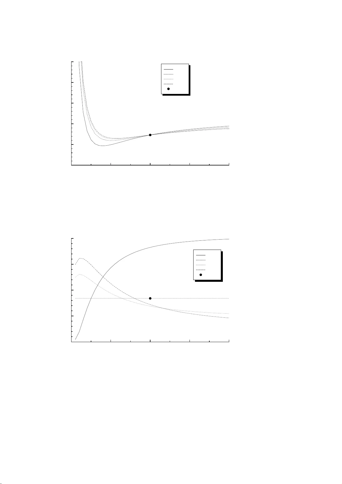
Explicit expressions for momen ts of the b eta W eibull distribution Gauss M. Cordei r o a, ∗ , Alexandr e B. Simas b, † and Bork o D. St o ˇ si ´ c a, ‡ a Departamen to de Estat ´ ıstica e Inform´ atica, Univ ersidade F ederal Ru ral de Pernam buco, Rua Dom Mano el d e Medeiros s/n, Dois Irm ˜ aos, 52171- 900 Recife-PE, Brasil b Asso cia ¸ c˜ ao Instituto Nacional d e Matem´ atica Pu ra e Aplicada, IMP A, Estrada D. Castorina, 110, Jd. Botˆ anico, 22460-3 20, Rio de J an eiro-RJ, Brasil Abstract The b eta W eibull d istr ibution was introd uced by F amo y e et al. (2005) and studied by these authors. Ho w ev er, they do not giv e explicit expressions for th e momen ts. W e no w derive explicit closed form expressions for the cu m ulativ e d istri- bution fun ct ion and for the moments of this distribution. W e also giv e an asymp- totic expansion for th e momen t generating function. F u rther, w e discu ss maxim u m lik elihoo d estimation and pro vide formulae for the element s of the Fisher informa- tion matrix. W e also demonstr at e the usefulness of this d istribution on a real data set. Keywor ds : Beta W eibull distribution, Fisher information matrix, Maxim um like li- ho od , Momen t, W eibull distrib u tio n. 1 In tro ductio n The W eibull distribution is a popular distribution widely used for analyzing lifetime data. W e w ork with the b eta W eibull (BW) distribution b ecause of the wide applicabilit y of the W eibull distribution and the fact tha t it extends some r ec en t dev elop ed distributions. This generalization may attra ct wider application in reliabilit y and biology . W e deriv e explicit closed form expressions for the distribution function and for the momen ts o f the BW distribution. An application is illustrat ed to a real data set with the hop e that it will attract mor e applications in reliability a nd biolog y , as w ell as in other areas of researc h. The BW distribution stems from the fo llo wing g eneral class: if G denotes the cu- m ulativ e distribution function (cdf ) of a r a ndom v aria ble then a generalized class of distributions can b e defined b y F ( x ) = I G ( x ) ( a, b ) (1) ∗ Corresp onding author. E-ma il: gaus scordeiro@uol.co m.br † E-mail: alesimas @impa.br ‡ E-mail: b orko@ufpe.br 1 for a > 0 and b > 0, where I y ( a, b ) = B y ( a, b ) B ( a, b ) = R y 0 w a − 1 (1 − w ) b − 1 dw B ( a, b ) is the incomplete b eta function ratio, B y ( a, b ) is the incomplete b eta f unc tion, B ( a, b ) = Γ( a )Γ( b ) / Γ( a + b ) is the b eta function and Γ( . ) is the gamma function. This class o f generalized distributions has b een receiving increased attention ov er the last y ears, in particular after the recen t works of Eugene et al. (200 2 ) and Jones (2004 ). Eugene et al. (2002) intro duce d what is kno wn as the b eta normal distribution by taking G ( x ) in (1) to b e the cdf of the normal distribution with parameters µ and σ . The only prop erties of the b eta normal distribution know n are some first moments deriv ed b y Eugene et a l. (2002) and some more general momen t expressions derived b y Gupta and Nadara jah (2004). More recen tly , Nadara jah and Ko tz (2004) were able to pro vide closed form expressions for the momen ts, the asymptotic distribution of the extreme order statistics and the estimation pro cedure fo r the b eta Gum b el distribution. Another distribution that happ ens to b elong to (1) is the log F (or b eta logistic) distribution, whic h has b een around for ov er 20 years (Bro wn et al., 2002), ev en if it did not originate directly fro m (1). While the transforma t io n (1) is not analytically tractable in the g ene ral case, the form ulae related with the BW turn out mana g eable (as it is sho wn in the rest of this pap er), and with the use of modern computer resources with analytic and n umerical capabilities, ma y turn in to adequate to ols comprising t he arsenal of applied statisticians. The curren t work represen ts an a dv ance in the direction traced b y Nadara jah and Kotz (2006), con trary to their b elief that some m athematical prop erties of the BW distribution are not tractable. Th us, follo wing (1) and replacing G ( x ) b y the cdf of a W eibull distribution with parameters c and λ , w e obtain the cdf of the BW distribution F ( x ) = I 1 − exp {− ( λx ) c } ( a, b ) (2) for x > 0, a > 0, b > 0, c > 0 and λ > 0. The corresp onding probability densit y f unction (p df ) and the ha zar d rat e function asso ciated with (2) are: f ( x ) = cλ c B ( a, b ) x c − 1 exp {− b ( λx ) c } [1 − exp {− ( λx ) c } ] a − 1 , (3) and τ ( x ) = cλ c x c − 1 exp {− b ( λx ) c } [1 − exp {− ( λx ) c } ] a − 1 B 1 − exp {− ( λx ) c } ( a, b ) , (4) resp ec tiv ely . Sim ulation from (3) is easy: if B is a random num b er follow ing a b eta distribution with parameters a and b then X = {− log (1 − B ) } 1 /c /λ will follo w a BW distribution with par a me ters a, b, c and λ . Some mathematical prop erties o f the BW distribution are given by F amo y e et al. (2005) and Lee et a l. (2 006). Graphical represen tation o f equations (3) and (4) for some choice s of parameters a and b , for fixed c = 3 and λ = 1, are giv en in Figures 1 and 2, respective ly . It should b e no t ed that a single W eibull distribution for the particular c hoice of the parameters c 2 and λ is here generalized by a f amily of curve s with a v a riet y of shap es, sho wn in these figures. The rest of the pap er is organized a s follo ws. In Section 2, w e obtain some expansions for the cdf of the BW distribution, and p oin t o ut some sp ecial cases that hav e b een considered in the literature. In Section 3, we deriv e explicit close d form expres sions for the momen ts and pres en t sk ewness and kurtosis for differen t parameter v alues. Section 4 giv es an expansion for its momen t generating function. In Section 5, w e discuss the maximum lik eliho od estimation and pro vide the elemen ts of the Fisher information matrix. In Section 6, an application to real data is presen ted, and finally , in Section 7, w e provide some conclusions. In the app endix, tw o identities needed in Section 3 are deriv ed. 0,0 0,5 1,0 1,5 2,0 2,5 3,0 0,0 0,2 0,4 0,6 0,8 1,0 1,2 1,4 1,6 1,8 2,0 a=0.5, b=0.5 a=2.0, b=2.0 a=0.5, b=2.0 a=2.0, b=0.5 Weibull f(x) x Figure 1: The probability densit y function (3) of the BW distribution, for sev eral v alues of para mete rs a a nd b 2 Expansions fo r the d istribution functio n The BW distribution is an extended mo del to analyze more complex data and g ene ralizes some recen t deve lop ed distributions. In particular, the BW distribution contains the exp o nen tiat ed W eibull distribution (for instance, see Mudholk ar et al., 1995, Mudholk ar and Hutson, 1996, Nassar and Eissa, 2003, Nadara ja h and Gupta, 200 5 and Choudh ury , 2005) as sp ecial cases when b = 1. The W eibull distribution (with pa r a mete rs c and λ ) is clearly a sp ecial case for a = b = 1. When a = 1, (3) follows a W eibull distribution with parameters λ b 1 /c and c . The b eta exp o nen tial distribution (Nadara ja h and Kotz, 2006) is also a sp ecial case for c = 1. In what follows , w e pro vide tw o simple form ulae for the cdf (2), dep ending on whe ther the parameter a > 0 is real non-inte ger or in teger, whic h ma y b e used for further analytical 3 0,0 0,5 1,0 1,5 2,0 2,5 0 1 2 3 4 5 a=0.5, b=0.5 a=2.0, b=2.0 a=0.5, b=2.0 a=2.0, b=0.5 Weibull W (x) x Figure 2 : The hazard func tion (4) o f the BW distribution, for sev eral v alues of parameters a a nd b or nume rical analysis. Starting from the explicit expression for the cdf ( 2 ) F ( x ) = cλ c B ( a, b ) Z x 0 y c − 1 exp {− b ( λy ) c } [1 − exp {− ( λy ) c } ] a − 1 dy , the change of v ariables ( λy ) c = u yields F ( x ) = 1 B ( a, b ) Z ( λx ) c 0 e − bu (1 − e − u ) a − 1 du. If a > 0 is real non-in teger w e hav e (1 − z ) a − 1 = ∞ X j =0 ( − 1) j Γ( a ) z j Γ( a − j ) j ! . (5) It follo ws that F ( x ) = 1 B ( a, b ) Z ( λx ) c 0 e − bu ∞ X j =0 ( − 1) j Γ( a ) e − j u Γ( a − j ) j ! du = 1 B ( a, b ) ∞ X j =0 ( − 1) j Γ( a ) Γ( a − j ) j ! Z ( λx ) c 0 e − ( b + j ) u du = 1 B ( a, b ) ∞ X j =0 ( − 1) j Γ( a ) Γ( a − j ) j !( b + j ) { 1 − e − ( b + j )( λx ) c } . 4 Finally , w e obtain F ( x ) = Γ( a + b ) Γ( b ) ∞ X j =0 ( − 1) j { 1 − e − ( b + j )( λx ) c } Γ( a − j ) j !( b + j ) . (6) F or p ositiv e r eal non-in teger a , the expansion (6) ma y be used for further ana lytical and/or nume rical studies. F or in teger a w e only need to c hange the formu la used in (5) to the binomial expansion to giv e F ( x ) = 1 B ( a, b ) a − 1 X j =0  a − 1 j  ( − 1) j { 1 − e − ( b + j )( λx ) c } ( b + j ) . (7) When b oth a and b = n − a + 1 ar e integers , the relatio n o f the incomplete b eta function to the binomial expansion giv es F ( x ) = n X j = a  n j  [1 − exp {− ( λx ) c } ] j exp {− ( n − j )( λx ) c } . (8) It can b e found in the W olfram F unctions Site 1 that for integer a I y ( a, b ) = 1 − (1 − y ) b Γ( b ) a − 1 X j =0 Γ( b + j ) y j j ! , and for integer b , I y ( a, b ) = y a Γ( a ) b − 1 X j =0 Γ( a + j )(1 − y ) j j ! . Then, if a is in teger, w e ha v e anot her equiv a lent f o rm for (7) F ( x ) = 1 − exp {− b ( λx ) c } Γ( b ) a − 1 X j =0 Γ( b + j ) j ! [1 − exp {− ( λx ) c } ] j . (9) F or in teger v alues of b , w e ha v e F ( x ) = [1 − exp {− ( λx ) c } ] a Γ( a ) b − 1 X j =0 Γ( a + j ) j ! exp {− j ( λx ) c } . (10) Finally , if a = 1 / 2 and b = 1 / 2, w e ha v e F ( x ) = 2 π arctan p exp { ( λx ) c } − 1 . (11) The par t icular cases (9) and (10) w ere discussed generally by Jones (2 0 04), and the ex- pansions (6)-(1 1 ) reduce to Nadar a jah and Kotz’s (2 0 06) results for t he b eta exp onen tia l distribution b y setting c = 1. Clearly , the expansions f or the BW densit y function are obtained fro m (6 ) and (7 ) b y simple differen tiation. Hence, the BW densit y function can b e expressed in a mixture form of W eibull densit y functions. 1 http:/ /function s.wolfram.com/GammaBetaErf/BetaRegularized/03/01/ 5 3 Momen ts Let X b e a BW random v ariable follow ing the densit y function (3). W e no w deriv e explicit expressions for the momen ts of X . W e now in tro duce the follow ing notatio n (f or an y r eal d and a and b p ositiv e) S d,b,a = Z ∞ 0 x d − 1 exp( − bx ) { 1 − exp( − x ) } a − 1 dx. (12) The c hange of v a riables x = − log ( z ) immediately yields S 1 ,b,a = B ( a, b ). On the other hand, the change of v a r ia bles x = ( λ y ) c giv es the fo llowing relation Z ∞ 0 y γ − 1 exp {− b ( λy ) c } [1 − exp {− ( λy ) c } ] a − 1 dy = λ − γ c S γ c ,b,a , (13) from whic h it follows that S γ /c,b,a = B ( a, b ) λ γ − c E ( X γ − c ) , or, equiv a len tly , fo r an y real r E ( X r ) = 1 λ r B ( a, b ) S r /c +1 ,b,a , (14) relating S r /c +1 ,b,a to the r th generalized momen t of the b eta W eibull. First, we consider the in tegral (12) when d is a n in teger. Let U b e a random v aria ble follo wing the Beta( b, a ) distribution with p df f U ( · ) and W = − log ( U ). F urther, let F U ( · ) and F W ( · ) b e the cdf ’s of U and W , respectiv ely . It is easy to see that F W ( x ) = 1 − F U ( e − x ). F urther, by the prop erties of the Leb esgue -Stiltjes integral, w e hav e E ( W d − 1 ) = Z ∞ −∞ x d − 1 dF W ( x ) = Z ∞ 0 x d − 1 e − x f U ( e − x ) dx = 1 B ( a, b ) Z ∞ 0 x d − 1 e − bx (1 − e − x ) a − 1 dx = S d,b,a B ( a, b ) . Th us, the v alues o f S d,b,a for in teger v a lues of d can be found from the moments of W if they are kno wn. How ev er, the moment g ene rating function (mgf ) M W ( t ) = E ( e tW ) of W can b e expressed as M W ( t ) = E ( U − t ) = 1 B ( a, b ) Z 1 0 x b − t − 1 (1 − x ) a − 1 dx = B ( b − t, a ) B ( a, b ) . This form ula is well defined for t < b . How ev er, w e are only in terested in the limit t → 0 and therefore this expression can b e used for the curren t purp ose. W e can write S d,b,a = B ( a, b ) E ( W d − 1 ) = B ( a, b ) M ( d − 1) W (0) = ∂ d − 1 ∂ t d − 1 B ( b − t, a )     t =0 . (15) 6 F rom equations (14) and (15) for an y p ositiv e integer k w e o bt a in a g ene ral formula E ( X k c ) = 1 λ k c B ( a, b ) ∂ k ∂ t k B ( b − t, a )     t =0 . (16) As part icular cases, w e can see directly from (15) that S 1 ,b,a = B ( a, b ) , S 2 ,b,a = B ( a, b ) { ψ ( a + b ) − ψ ( b ) } and S 3 ,b,a = B ( a, b ) [ ψ ′ ( b ) − ψ ′ ( a + b ) + { ψ ( a + b ) − ψ ( b ) } 2 ] , and b y using (14) w e find E ( X c ) = { ψ ( a + b ) − ψ ( b ) } λ c and E ( X 2 c ) = ψ ′ ( b ) − ψ ′ ( a + b ) + { ψ ( a + b ) − ψ ( b ) } 2 λ 2 c . The same results can also b e obtained directly f rom (16). Note that the formula for S 1 ,b,a matc hes the one just given after equation (12). Since the BW distribution for c = 1 reduces to the b eta exp onen tial distribution, the ab o v e form ulae fo r E ( X c ) and E ( X 2 c ) reduce to the corresp onding ones obtained by Nadara jah and Kotz (200 6 ). Our main g oal here is to giv e the r th momen t o f X for ev ery p ositiv e integer r . In fact, in what follo ws w e obtain the r th generalized momen t fo r ev ery real r whic h ma y b e used for further theoretical or n umerical analysis. T o this end, we need to obta in a form ula for S d,b,a that holds for ev ery p ositiv e real d . In the app endix w e sho w that for an y d > 0 t he following iden tit y holds for p ositiv e real non- in teger a S d,b,a = Γ( a )Γ ( d ) ∞ X j =0 ( − 1) j Γ( a − j ) j !( b + j ) d (17) and that when a is po s itiv e in teger S d,b,a = Γ ( d ) a − 1 X j =0  a − 1 j  ( − 1) j ( b + j ) d (18) is satisfied. It no w follows from (17) and (14) tha t the r t h generalized momen t o f X for p ositiv e real non-in teger a can b e written as E ( X r ) = Γ( a )Γ( r /c + 1) λ r B ( a, b ) ∞ X j =0 ( − 1) j Γ( a − j ) j !( b + j ) r /c +1 . (19) When a > 0 is inte ger, we obtain E ( X r ) = Γ( r /c + 1) λ r B ( a, b ) a − 1 X j =0  a − 1 j  ( − 1) j ( b + j ) r /c +1 (20) 7 When a = b = 1, X follows a W eibull distribution and (20) b ecomes E ( X r ) = Γ( r /c + 1) λ r , whic h is precisely the r th mo ment of a W eibull distribution with parameters λ and c . Equations (1 6), (19) and (2 0) represen t the main results of this section, whic h may serv e as a starting p oin t for applications for particular cases as w ell as further researc h. 0,0 0,5 1,0 1,5 2,0 0,0 0,5 1,0 1,5 b=0.5 b=1.0 b=1.5 b=2.0 Weibull skewness a Figure 3: Sk ewnes s of the BW dis tribution as a function of parameter a , for sev eral v alues of para mete r b Graphical represen tation o f sk ewne ss and kurtosis for some ch oices of parameter b as function of parameter a , and fo r some choic es of parameter a as function of parameter b , for fixed λ = 1 and c = 3, are giv en in F igures 3 and 4, and 5 a nd 6, respectiv ely . It can b e observ ed fr om Figures 3 and 4 that the sk ewne ss and kurtosis curv es cross at a = 1, and from Figures 5 and 6 that b oth sk ewness and kurtosis are indep enden t o f b for a = 1. In addition, it should b e noted that the W eibull distribution (equiv alent t o BW f o r a = b = 1) is represen ted by as single p oin t on Figures 3 -6. 8 0,0 0,5 1,0 1,5 2,0 -1,0 -0,5 0,0 0,5 1,0 1,5 b=0.5 b=1.0 b=1.5 b=2.0 Weibull kurtosis a Figure 4 : Kurtosis o f the BW distribution as a function of pa rameter a , for sev eral v alues of para mete r b 0,0 0,5 1,0 1,5 2,0 0,0 0,1 0,2 0,3 0,4 a=0.5 a=1.0 a=1.5 a=2.0 Weibull skewness b Figure 5: Sk ewness of the BW distribution as a function of parameter b , for sev eral v a lues of para mete r a 9 0,0 0,5 1,0 1,5 2,0 -0,6 -0,5 -0,4 -0,3 -0,2 -0,1 0,0 a=0.5 a=1.0 a=1.5 a=2.0 Weibull kurtosis b Figure 6 : Kurto sis of the BW distribution as a function of parameter b , f or sev eral v alues of para mete r a 4 Momen t Gener ating F unction W e can giv e an expansion f or the mgf of the BW distribution as follows M ( t ) = cλ c B ( a, b ) Z ∞ 0 exp( tx ) x c − 1 exp {− b ( λx ) c } [1 − exp {− ( λx ) c } ] a − 1 dx = cλ c B ( a, b ) ∞ X r =0 t r r ! Z ∞ 0 x r + c − 1 exp {− b ( λx ) c } [1 − exp {− ( λx ) c } ] a − 1 dx = cλ c B ( a, b ) ∞ X r =0 t r r ! λ − ( r + c ) c S r /c +1 ,b,a , where the last expression comes from (13). F or p ositiv e real non- in teger a using (17) w e ha v e M ( t ) = Γ( a ) B ( a, b ) ∞ X r =0 ∞ X j =0 t r Γ( r /c + 1)( − 1) j λ r Γ( a − j )( b + j ) r /c +1 r ! j ! , (21) and for integer a > 0 using (18) we obtain M ( t ) = 1 B ( a, b ) ∞ X r =0 t r Γ( r /c + 1) λ r r ! a − 1 X j =0  a − 1 j  ( − 1) j ( b + j ) r /c +1 . (22) 10 Note that the expression f o r the mgf obtained by Choudh ury (2005) is a part icular case of (2 1 ), when a = θ , λ = 1 /α and b = 1. When c = 1, w e ha v e M ( t ) = ∞ X r =0 λ − r t r cB ( a, b ) r ! S r +1 ,b,a = λ B ( a, b ) Z ∞ 0 e tx − bλx (1 − e − λx ) a − 1 dx. Substituting y = exp( − λx ) in the ab o v e integral yields M ( t ) = 1 B ( a, b ) Z 1 0 y b − t/λ − 1 (1 − y ) a − 1 dy (23) and using the definition of the b eta function in (2 3 ) w e find M ( t ) = B ( b − t/λ, a ) B ( a, b ) , whic h is precisely the expression (3.1) obtained b y Nadara jah and Kotz (2006 ). 5 Estimation and i nformation matrix Let Y be a random v ariable with the BW distribution (3 ). The log -lik elihoo d for a single observ ation y of Y is given b y ℓ ( λ, c, a, b ) = log( c ) + c log ( λ ) + ( c − 1)log ( y ) − log { B ( a, b ) } − b ( λy ) c + ( a − 1)log [1 − exp {− ( λy ) c } ] . The corresp o nding comp onen ts o f the score vec tor are: ∂ ℓ ∂ a = − { ψ ( a ) − ψ ( a + b ) } + log n 1 − e − ( λ y ) c o , (24) ∂ ℓ ∂ b = − { ψ ( b ) − ψ ( a + b ) } − ( λ y ) c , (25) ∂ ℓ ∂ c = 1 c + log ( λ y ) − b ( λ y ) c log ( λ y ) + ( a − 1) ( λ y ) c log ( λ y ) e − ( λ y ) c 1 − e − ( λ y ) c (26) and ∂ ℓ ∂ λ = c λ − b c λ ( λ y ) c + c ( a − 1 ) ( λ y ) c e − ( λ y ) c λ { 1 − e − ( λ y ) c } . (27) The maxim um lik elihoo d equations deriv ed by equating (24)-(27) to zero can b e solv ed n umerically for a, b, c and λ . W e can use iterative techniq ues suc h as a Newton-Raphson t yp e algorit hm to obtain t he estimates o f these pa rameters . It ma y b e worth noting fro m E ( ∂ ℓ/∂ b ) = 0, that (2 5 ) yields E ( Y c ) = ψ ( a + b ) − ψ ( b ) λ c , 11 whic h agrees with the previous calculations. F or interv al estimation of ( a, b, c, λ ) and h yp othes is tests, the F ish er info rmation ma- trix is required. F o r expressing the elemen ts o f this matrix it is conv enien t to in tro duce an extension of the in tegral (12) T d,b,a,e = Z ∞ 0 x d − 1 e − bx  1 − e − x  a − 1 (log x ) e dx, (28) so t ha t we hav e T d,b,a, 0 = S d,b,a . As b efore, let W = − log( U ), where U is a rando m v ariable following the Beta( b, a ) distribution, then E [ W d − 1 { log( W ) } e ] = Z ∞ −∞ x d − 1 (log x ) e dF W ( x ) = 1 B ( a, b ) Z ∞ 0 x d − 1 e bx (1 − e − x ) a − 1 (log x ) e dx = T d,b,a,e B ( a, b ) . Hence, t he equation T d,b,a,e = B ( a, b ) E [ W d − 1 { log( W ) } e ] , (29) relates T d,b,a,e to exp ected v a lues. T o simplify the expressions for some elemen ts of the informat io n matrix, it is useful to note the iden tities S 1 ,b +2 ,a − 2 S 1 ,b +1 ,a + S 1 ,b,a = B ( a + 2 , b ) and bS 2 ,b,a − ( a + 2 b + 1) S 2 ,b +1 ,a + ( a + b + 1 ) S 2 ,b +2 ,a = B ( a + 2 , b ) , whic h can b e easily pro v ed. Explicit express ions for the elemen ts of the information matrix K , obtained using Maple and Mathematica a lg ebraic manipulation soft w are (w e ha v e used b oth for double c hec king the obtained express ions), are giv en b elow in terms of the in tegrals (1 2) and (28): κ a,a = ψ ′ ( a ) − ψ ′ ( a + b ) , κ a,b = − ψ ′ ( a + b ) , κ a,c = − T 2 ,b +1 ,a − 1 , 1 cB ( a, b ) , κ a,λ = − c S 2 ,b +1 ,a − 1 λB ( a, b ) , κ b,b = ψ ′ ( b ) − ψ ′ ( a + b ) , κ b,c = T 2 ,b,a, 1 cB ( a, b ) , κ b,λ = c λ S 2 ,b,a B ( a, b ) , 12 κ c,c = 1 c 2 + 1 c 2 B ( a, b ) { ( a − 1) T 3 ,b +1 ,a − 2 , 2 + b T 2 ,b,a − 2 , 2 − ( a + 2 b − 1) T 2 ,b +1 ,a − 2 , 2 + ( a + b − 1) T 2 ,b +2 ,a − 2 , 2 } , κ c,λ = 1 λ B ( a, b ) { ( a − 1 ) T 3 ,b +1 ,a − 2 , 1 + b T 2 ,b,a − 2 , 1 − ( a + 2 b − 1) T 2 ,b +1 ,a − 2 , 1 + ( a + b − 1) T 2 ,b +2 ,a − 2 , 1 } and κ λ,λ = c 2 λ 2 + c 2 ( a − 1) λ 2 B ( a, b ) S 3 ,b +1 ,a − 2 . The in tegrals S i,j,k and T i,j,k ,l in the information matrix are easily n umerically determined using MAPLE and MA THEMA TICA for an y a and b . Under conditio ns that are fulfilled fo r parameters in the in terior o f the parameter space but no t on the bo undar y , the asymptotic distribution of t he maxim um lik eliho o d estimates ˆ a, ˆ b, ˆ c and ˆ λ is m ultiv ariate normal N 4 (0 , K − 1 ). The estimated multiv ariate normal N 4 (0 , b K − 1 ) distribution can b e used to construct appro ximate confidenc e in terv als and confidence regions f o r the individual parameters and for the hazard r a te and surviv al functions. The asymptotic normality is also useful for testing go o dness o f fit of the BW distribution a nd for comparing t his distribution with some of its sp ecial sub-mo dels using one of the three w ell-kno wn asymptotically equiv alen t test statistics - namely , the lik eliho od ratio (LR) statistic, W ald and Rao score statistics. W e can compute the maxim um v alues of the unre stricted and restricted log-lik eliho ods to construct the LR statistics for testing some sub-mo dels of the BW distribution. F o r example, we ma y use the L R statistic to che c k if the fit using t he BW distribution is statistically “sup erior” to a fit using the exponen tiated W eibull or W eibull distributions for a giv en data set. Mudholk ar et al. (1995) in their discussion of the c lassical bus-motor- failure data, noted the curious asp ect in whic h the la rger EW distribution provide s a n inferior fit as compared to the smaller W eibull distribution. 6 Applicatio n to real data In this sec tion we compare the results o f fitting the BW and W eibull distribution to the data set studied by Meek er and Escobar (1998, p. 383), whic h give s the times of failure and running times for a sample of devices fr o m a field-trac king study of a larger system. A t a certain p oin t in time, 30 units w ere installed in normal service conditions. Tw o causes of failure w ere observ ed f o r eac h unit that f a iled: the fa ilure caused b y an accum ulation of randomly o ccurring damage from p ow er-line v oltage spik es during electric storms and failure caused b y normal pro duct wear. The times a r e: 275, 13, 147, 23, 181, 30, 65, 10, 300, 173, 106, 300, 300, 212 , 300, 300 , 300, 2 , 2 61, 293 , 8 8, 247, 28, 143, 300, 23, 3 0 0, 80, 245, 2 66. 13 The maximum like liho o d estimates and the maximized log-likelihoo d ˆ l B W for the BW distribution are: ˆ a = 0 . 0785 , ˆ b = 0 . 0659 , ˆ c = 7 . 9355 , ˆ λ = 0 . 00 4987 and ˆ l B W = − 169 . 9 19 , while the maxim um lik elihoo d estimates and the maximized log-like liho o d ˜ l W for the W eibull distribution are: ˜ c = 1 . 26 50 , ˜ λ = 0 . 00531 8 and ˜ l W = − 184 . 3 138 . The like liho o d ra tio statistic for testing the h yp othesis a = b = 1 (namely , W eibull v ersus BW distribution) is then w = 28 . 7 896, whic h indicates that the W eibull distribu- tion should b e rejected. As an alternativ e test w e use the W ald stat is tic. The asymptotic co v ariance matrix o f the maxim um lik eliho o d estimates fo r the BW distribution, whic h comes from the in v erse of the info r ma t io n matrix, is g iv en by b K − 1 = 10 − 7 ×     8699 . 3536 4 4743 . 6997 7 − 488130 . 870 87 . 9136383 4743 . 6997 7 13079 . 439 4 − 4009 . 69885 − 135 . 6033 33 − 488130 . 870 − 400 9 . 69885 5851 7447 . 8 − 16222 . 8149 87 . 913638 3 − 135 . 603333 − 162 2 2 . 8149 6 . 195 30131     . The resulting W a ld statistic is found to b e W = 38 . 4498 , a gain signalizing that the BW distribution conform to the ab o v e data. In Figure 7 w e displa y the p df o f b oth W eibull and BW distributions fitted and the data set, w here it is seen that the BW mo del captures the a paren t bimo dality of the da t a. 0 20 40 60 8 0 100 120 140 160 180 200 220 240 260 280 300 0,000 0,005 0,010 Data points Weibull Beta Weibull fdp y Figure 7: The probabilit y density function (3 ) of the fitted BW a nd W eibull distributions 14 7 Conclus ion The W eibull distribution, having exponential and Ra yleigh as sp ecial cases , is a v ery p op- ular distribution for mo deling lifetime data and for mo deling phenomenon with mono- tone failure rates. In fa ct, the BW distribution represen t s a generalization of sev eral distributions previously considered in the literature suc h as the exp onen t ia ted W eibull distribution (Mudholk ar et al., 1995, Mudholk ar and Hutson, 1 996, Nassar and Eissa, 2003, Nadara jah and Gupta, 2005 and Choudhu ry , 2005 ) obtained when b = 1 . The W eibull distribution (with parameters c and λ ) is a lso anot her particular case f or a = 1 and b = 1. When a = 1, the BW distribution reduces to a W eibull distribution with parameters λ b 1 /c and c . The b eta exp onen tial distribution is also an imp ortan t sp ecial case for c = 1 . The BW distribution provide s a rather general and flexible framew ork for statistical analysis. It unifi es sev eral previously prop osed families of distributions, therefore yielding a g en eral o v erview of these families for theoretical studies, and it also prov ides a rather flexible mechanis m for fitting a wide sp ectrum of real w orld data sets. W e deriv e explicit expressions for the momen ts of the BW distribution, including an expansion for the moment g enerating function. These express ions a re manageable and with the use of mo dern computer resources with ana lytic and nume rical capabilities, ma y turn in to adequate to ols comprising the arsenal of applied statisticians. W e discus s the estimation pro cedure by maxim um lik eliho o d and deriv e the information matrix. Finally , w e demonstrate an application to real data. App end ix In what follows, w e deriv e the identities ( 1 7 ) and (1 8). W e start from f ( x ) = exp( − bx )(1 − e − x ) a − 1 , whic h yields Z ∞ 0 x d − 1 f ( x ) dx = Z ∞ 0 x d − 1 exp( − bx )(1 − e − x ) a − 1 dx, and substituting z = e − x giv es Z ∞ 0 x d − 1 f ( x ) dx = Z 1 0 | log z | d − 1 z b − 1 (1 − z ) a − 1 dz . (30) F or real no n- in teger a , w e ha v e Z ∞ 0 x d − 1 f ( x ) dx = Γ( a ) ∞ X j =0 ( − 1) j Γ( a − j ) j ! Z 1 0 | log z | γ /c − 1 z b + j − 1 dz . Also, f o r r eal p > − 1 and real q , w e ha v e Z 1 0 x p | log x | q dx = Γ(1 + q ) (1 + p ) q +1 . (31) 15 Hence, Z ∞ 0 x d − 1 f ( x ) dx = Γ( a ) ∞ X j =0 ( − 1) j Γ( d ) Γ( a − j ) j !( b + j ) d , and, finally , w e arrive at Z ∞ 0 x d − 1 exp( − bx )(1 − e − x ) a − 1 dx = Γ( a )Γ ( d ) ∞ X j =0 ( − 1) j Γ( a − j ) j !( b + j ) d , whic h represen t s the identit y (17). No w, let a > 0 b e an integer; then, from (30), w e hav e Z ∞ 0 x d − 1 f ( x ) dx = a − 1 X j =0  a − 1 j  ( − 1) j Z 1 0 | log z | d − 1 z b + j − 1 dz . Using (3 1) w e obtain Z ∞ 0 x d − 1 f ( x ) dx = a − 1 X j =0  a − 1 j  ( − 1) j Γ( d ) ( b + j ) d , and therefore we arriv e at Z ∞ 0 x d − 1 exp( − bx )(1 − e − x ) a − 1 dx = Γ ( d ) a − 1 X j =0  a − 1 j  ( − 1) j ( b + j ) d , whic h represen t s the identit y (18). References [1] Brow n, B. W., Spears, F. M. a nd Levy , L. B. (2002). The log F : a distribution fo r all seasons. Comput. Statist. , 17, 47-58 . [2] Choudh ury , A., 2 005. A simple deriv ation of momen ts of t he exp onen t ia ted W eibull distribution. Metrika , 62 , 1 7 -22. [3] Eugene, N., Lee, C. and F amo y e, F., 2 002. Beta- normal distribution a nd its a ppli- cations. C ommun. Statist. - The o ry and Metho ds , 31, 497-512 . [4] F amo y e, F., Lee, C. and Olumolade, O., 20 05. The Beta-W eibull Distribution. J. Statistic al The ory and Applic ations , 4, 121-136 . [5] Gupta, R. D . a nd Kundu, D., 2001. Exp onen tiated Expo nen tial F amily: An Alter- nativ e to Gamma and W eibull D istributions. Biometric al Journal , 43, 1 17-130. [6] Gupta, A. K. and Nada ra jah, S., 200 4 . On the momen ts of the b eta normal distri- bution. Commun. Statist. - The ory and Metho ds , 3 3, 1-13. 16 [7] Jones, M. C., 2004 . F amilies o f distributions arising from distributions of o rder statis- tics. T est , 13, 1 - 43. [8] Law less, J. F., 1982. Statistic al Mo d els a nd Metho ds for Lifetime Data . John Wiley , New Y ork. [9] Lee, C., F amo y e, F. and Olumolade, O., 2007. Beta-W eibull Distribution: Some Prop erties and Applications to Censored D ata. J. Mo de rn Applie d Statistic al Meth- o ds , 6, 173- 186. [10] Linhart, H. and Zucc hini, W., 19 8 6. Mo del Sele ction. John Wiley , New Y ork. [11] Meek er, W. Q. a nd Escobar, L. A., 1998. Statistic al Metho ds for R eliability Da ta . John Wiley , New Y ork. [12] Mudholk ar, G. S., Sriv astav a, D. K. and F reimer, M., 1995. The exp onen tia ted W eibull family . T e chnometrics , 37, 436-4 5. [13] Mudholk ar, G. S. a nd Hutson, A. D ., 199 6. The exp onen tiated W eibull family: some prop erties a nd a flo od data application. Com mun. S tat ist. - The ory and Metho ds , 25, 30 59-3083. [14] Nadara jah, S. and Gupta, A. K., 2005. On the moments of the exp onen tiated W eibull distribution. C ommun. Statist. - The o ry and Metho ds , 34, 253-2 5 6. [15] Nadara jah, S. and Kotz, S., 2004. The b eta Gumbel distribution. Math. Pr ob ab. Eng. , 10 , 3 2 3-332. [16] Nadara jah, S. and Kotz, S., 2006. The b eta exp onen tial distribution. R eliability Engine ering and System Safety , 91, 689-69 7 . [17] Nassar, M. M. and Eissa, F. H., 20 03. On the exp onen tiated W eibull distribution. Commun. Statist. - The ory and Metho ds , 32, 131 7-1336. 17