Another approach to decide on real root existence for univariate Polynomials, and a multivariate extension for 3-SAT

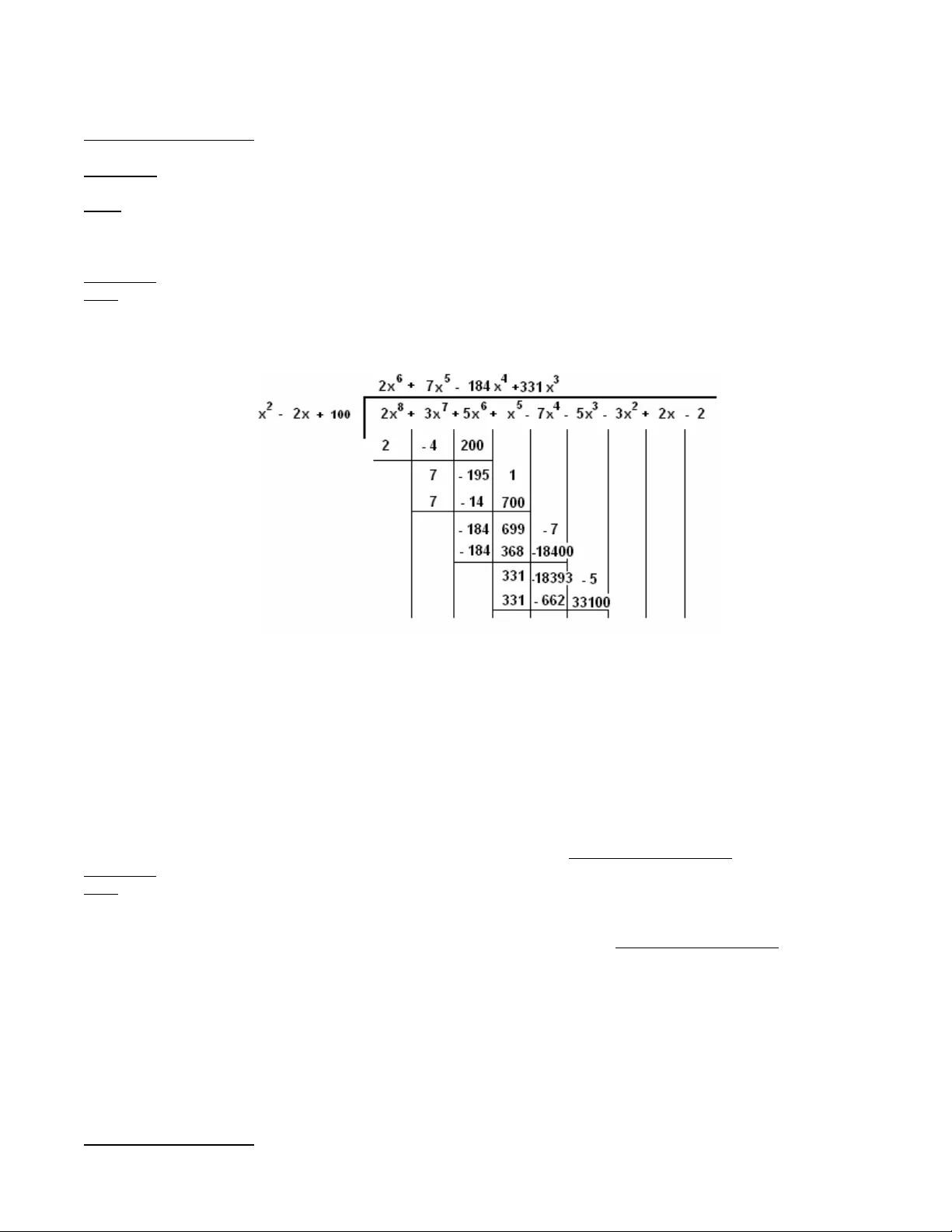
Another approach t o decide on real root existence for univ ariate Polynom ials, and a multivariate extens ion for 3-SAT Deepak Ponvel Chermakani, IEEE Member deepakc@pmail.ntu.edu.sg deepakc@myfastmail.co m deepakc@usa.com deep ak.chermakani@ ust-global.co m Abstract: - We present six Theorems on the univar iate real Polynomial, using which we develop a new algorit hm for deciding the existence of atleast one real root for univariate integer Polynomials. Our algorithm outputs that no positive real root exists, if and only if, the given Polyno mial is a factor of a real Polynomial with positive coefficient s. Next, we define a transformation that transforms any instance of 3-SAT into a multivariat e real Polynomial with positive coefficients, if and only if, the instance is not satisfiable. 1. Introduction One can decide within pol ynomial time, whether or not a univariate Pol ynomial with integer coefficient s has a real root [1]. However, as the number of variables in the Polyno mial incr ease, the complexit y of deciding on existence of a real root increases exponentially with the number of variables. I n this paper, we shall de velop a ne w approach for decid ing on existe nce of a real roo t in the univariate case, and shall analyze its extension to the multivariate case of 3-SAT . We denote an “Integer Pol ynomial” as a Polynomial having integer coe fficients, and a “Real Polynomial” as a P olyno mial having real coefficients. In the next Section 2, we shall state six theorems on the univariate real Pol ynomial, using which we shall then construct a n algorithm in Section 3, for deciding on existence of a real ro ot in a univariate integer Polyno mial. In Section 4, we shall define a transformation that transfor ms any instance of 3 -SAT into a multivariate real Pol ynomial with positi ve coe fficients, i f a nd onl y if, the instance is not satisfiable. 2. Six Theorems on the univariate real Polynomial The given univariate integer P olynomial, for which we are tr ying to decide on existence of a real ro ot, is of the following form: P(X) = a 0 + a 1 X + a 2 X 2 + a 3 X 3 + … a N X N , where N is P’s degree, where the set {a 0 , a 1 , …a N } belongs to the set of Integer s, where M is the maximum magnitude of elements in {a 0 , a 1 , …a N }, and finally where β repre sents either the lo wer bound of the magnitude of the non-zero i maginary co mponent, or the lo wer bo und of the magnitude o f the non-zero r atio bet ween the imaginary co mponent and corresponding real co mponent, in the co mplex roots of P(X). Theorem-1: There exists a real Polynomial R(X) of degree equal to (1 + INT ( π p/q)), with positive coefficients, which when multiplied with the Quadratic ((X – p) 2 + q 2 ) where p and q are positive real numbers, gives a resultant real Polyno mial having positive coefficients. Proof : We are trying to find the required degree D, of the polynomial R(X) = X D + C 1 X D-1 + C 2 X D-2 + C 3 X D-3 + … C D , with real coefficients, which when multiplied with ((X – p) 2 + q 2 ), gives a resultant Polynomial with positive coefficients. We procee d by proving 2 Lemmas. Lemma-1.1 : This required degree D, of R(X) is independe nt of the individual numerical values of p and q, and only depends on the ratio p:q. The higher this r atio, the greater is D Proof : Consider the product of the quadratic (X 2 – 2pX + (p 2 + q 2 )) with R (X). If <1, r 1 , r 2 … r D+2 > depicts the coefficient s of , in this product, then we have: r 1 = C 1 – 2p r 2 = C 2 – 2pC 1 + (p 2 + q 2 ) r 3 = C 3 – 2pC 2 + C 1 (p 2 + q 2 ) … r i = C i – 2pC i-1 + C i-2 (p 2 + q 2 ) … r D = C D – 2pC D-1 + C D-2 (p 2 + q 2 ) r D+1 = – 2pC D + C D-1 (p 2 + q 2 ) r D+2 = C D (p 2 + q 2 ) Since each of {1, r 1 ,… r D+2 } needs to be > 0 by a small amount, then as r i  0, for all i in [1,N], we can obtain the follo wing (by starting from C 1 and iterativel y substituting the value of C i-2 and C i-1 in the subseque nt value of C i ): C 1 = 2p + µ 1 C 2 = (2p) 2 – (p 2 + q 2 ) + µ 2 C 3 = (2p) 3 – 2(2p)(p 2 + q 2 ) + µ 3 C 4 = (2p) 4 – 3(2p) 2 (p 2 + q 2 ) + (p 2 + q 2 ) 2 + µ 4 C 5 = (2p) 5 – 4(2p) 3 (p 2 + q 2 ) + 3(2p)(p 2 + q 2 ) 2 + µ 5 In the previously mentione d sequence of C i , the quantitie s µ 1 , µ 2 , µ 3 , etc, are positive a nd  0. If we denote the ratio of p:q as h, then the pr eviously mentioned seq uence of C i beco mes: C 1 = 2p + ∆ 1 C 2 = p 2 ((2) 2 – (1 2 + h 2 )) + ∆ 2 C 3 = p 3 ((2) 3 – 2(2)(1 2 + h 2 )) + ∆ 3 C 4 = p 4 ((2) 4 – 3(2) 2 (1 2 + h 2 ) + (1 2 + h 2 ) 2 ) + ∆ 4 C 5 = p 5 ((2) 5 – 4(2) 3 (1 2 + h 2 ) + 3(2)(1 2 + h 2 ) 2 ) + ∆ 5 … where the quantities ∆ 1 , ∆ 2 , ∆ 3 , ∆ 4 , etc, are positive and  0. By induction, it is straightfo rward to obtain the result that the sign of C i is independe nt of the individual values of p or q, but only depends on the ratio p:q. And what is actually require d is that C D is just negative, which will mean that D is the degree of R(X) that is just sufficient to ensure that all the coefficien ts of the resultant pol ynomial are just sufficientl y above zero . The reason is that i f C D is just negative, t hen we ca n force C D = 0, making r D+2 = 0, and r D+1 = some po sitive value b ecause C D-1 i s still positive, and finally r D-2 is ob viously some small positive quantity. Thus, D depends onl y on the ratio p:q. Further, it is obvious that suppose if we were to force q=0, then there can exist no expression R(X) with a finite degree, that can force the product of R(X) and (X 2 – 2pX + p 2 ) to have zero sign cha nges in its coefficients, because by Descartes Rule of Signs, we know that (X 2 – 2pX + p 2 ) has 2 real roots, and therefore the prod uct of R(X) with (X 2 – 2pX + p 2 ) must also have atleast 2 sign changes while reading its coefficients. Then, as the ratio p:q keeps increasi ng; the required val ue of D als o increases. Hence Pro ved Lemma-1.1 Lemma-1.2: The re quired de gree D of R(X) is bounded b y the product of the ratio p:q and the irrational π (which is 3 .141592 …). Proof : To prove this, we first look at the sequence S i obtained while derivin g the value of π [2]. Next, w e will show that for the case of a=p=½, the terms of our sequence C i (that we introduced in Lemma-1.1) decreases faster than S i , and that C 1 = S 1 , and also that C 2 < S 2 . Finally, we invoke Lemma -1.1, to show that sequence C i decreases faster than S i irrespecti ve of the value of p. Consider a circle of radius a, centered at (0, a), where we are trying to inscribe triangles in the right half of the circle wrt Y- axis. Let us consider 2 such tri angles as sho wn in the belo w figure-1. Fig 1. Two inscribed triangles being considered In the above figure-1, angles AOB and BOC ar e denoted to b e eq ual to 2 ∂, and the angle between O A and Y -axis i s denoted to be equal to ℮. Let u s denote S i , S i+1 , and S i+2 as the lengths of the proj ections of OA, OB , and OC respectively on the Y-axis, and let us also denote the lengths o f segments AB=BC=b/2. Then we ob tain 4 equations: sin ( ∂) = b / 4a S i – a = a cos ( ℮) S i+1 – a = a cos ( ℮ + 2∂) S i+2 – a = a cos ( ℮ + 4∂) Simplifying the previous 4 equations yields the relation ship: S i+2 = 2 S i+1 (1 – b 2 /(8a 2 )) – S i + b 2 /(4a) If we put a=½, a nd simplify then it becomes S i+2 = 2 S i+1 (1 – b 2 /2) – S i + b 2 /2 Let us revisit the derivatio n of the irrational π . As we go on inscribing more and more small triangles, where the top most triangle touches X=1, and the bottom most triangle touches X=0, then as b  0, the number of such triangles being ‘n’, then using the formula for the length of half of the circumference of a circle, w e can say that nb/2 = π /2, or n= π /b. We have S 1 =1 (since the Y-projection of the tip of the to p most triangle meets the Y-axis at 1). Looking back at our original sequence, since C i – 2pC i-1 + C i-2 (p 2 + q 2 ) is almost zero, then putting p=½ and replacing i with i+2, w e get C i+2 = C i+1 – C i (q 2 + ¼), and w e also get C 1 = 1 (which is equal to S 1 ), and C 2 = ¾ – q 2 (which is lesser than S 2 , because S 2 is supposed to b e very close to S 1 =1, when b  0). It is easy to see that when C i and S i are both positive, then C i > C i+1 > C i+2 , and S i > S i+1 > S i+2 . Now, we will go on to prove that the rate at which C i decreases is faster than the rate at which S i decreases, which, coupled with the fact that S i reaches zero when i > π /b, would enable us to conclude that C i will also become negative be fore i > π /q, as q  0. This pro of is as follo ws. We have the 2 seq uences, when a=p=½: S i+2 = 2 S i+1 (1 – b 2 /2) – S i + b 2 /2, being the first sequence, and, C i+2 = C i+1 – C i (b 2 + ¼), being the second seq uence. (note tha t we are replacin g q with b, as both quantities  0) Adding and subtracting terms, we can say that S i+2 = S i+1 – S i (b 2 + ¼) + (1-b 2 )S i+1 – S i (¾ - b 2 ) + b 2 /2. Now S i decreases at a slower rate than C i , if (1-b 2 )S i+1 – S i (¾ - b 2 ) + b 2 /2 > 0 , which is true if S i+1 – ¾ S i + b 2 (½ – S i+1 + S i ) > 0 . I t is easy to s ee that it is true, because the coefficient of b 2 is positive, and because the value of S i+1 – ¾ S i is also positive, as S i+1 is lesser than S i by a quantity less than b which we have assumed to b e very s mall. T hus, C i beco mes negative before i > INT( π /b), or INT( π /q). In our entire argument above, we have assu med that p = ½. However, even if p ≠ ½, we may recall from Lemma-1.1 , that the event of C i becoming just negative does not depend on p or q, but only on the ratio p:q, hence we can directly conclud e that C i will beco me negative before i > π (p/q). Hence Pro ved Lemma-1.2 Lemma-1.1 and Lemma-1.2 , complete the proo f of Theor em-1. However, for verification, we have pasted computer simulations in T able-1, regarding when sequence C i beco mes negative, and it is i nteresting to see that (i/(p/q )) do es tend to π . Finally, it is also obvious that not only does the resulting Polynomial (prod uct of the Quadratic with R(X)) have positive coefficients, but also R(X) itse lf has positive co efficients. Hence Proved Theore m-1 Table 1. Computer simulation results for checking when C i just becomes negative p/q i at which C i just becomes negative 1 3 2 6 3 9 4 12 6 19 8 25 9 28 12 37 13 40 15 47 19 59 20 62 30 94 34 106 36 113 40 125 41 128 49 153 50 157 51 160 100 314 200 628 1,000 3141 10,000 31415 100,000 314159 1,000,000 3141592 Theorem-2: Let Q(X) be a real polyno mial. Deciding on real root existence for the given univariate polyno mial Q(X), is equivalent to deciding the sa me for ((X – p 1 ) 2 + q 1 2 ) ((X – p 2 ) 2 + q 2 2 ) ((X – p 3 ) 2 + q 3 2 )…((X – p N ) 2 + q N 2 ) = 0, w here {p 1 , p 2 , … p N } belongs to the set o f real numbers, a nd where { q 1 , q 2 , … q N } belongs to the set o f non-nega tive rea l numbers. Proof : Whether or not Q(X)=0 is solvable in a real interval, is equivalent to whether or not Q 2 (X)=0 is solvable in that same real interval. Next, we know that the real roots of a polynomial may o r may not be repeated , and that the complex roots must occur in conjugate pairs. Therefore , when we square Q(X), we obtain a prod uct of N quadratic compo nents: ((X – p 1 ) 2 + q 1 2 ) ((X – p 2 ) 2 + q 2 2 ) ((X – p 3 ) 2 + q 3 2 )….. ((X – p N ) 2 + q N 2 ), where {p 1 , p 2 , … p N } belongs to the set of real numbers, and where {q 1 , q 2 , … q N } belongs to the set of non-negative r eal number s. Hence Proved Theore m-2 Theorem-3: Let Q(X) be a rea l polyno mial. In those qua dratic components of Q 2 (X), ((X – p i ) 2 + q i 2 ) where p i and q i are positive real numbers, the magnitude of the rat io p i :q i is bounded below (2 β - 1 (MN) 2 ). Proof : Let us denote one of the factor polynomials of P 2 (X), to be P 1 (X), a polynomial with real coefficients. We denote K as the degree of P 2 (X), and L as the maximum coefficie nt of P 2 (X). Then it is clear that K=2 N, and L< NM 2 . We also define “coefficient normalization” of a pol ynomial, as the multiplication of every coefficient by a real, such that the smallest non-zero magnitude of coefficients i n the polyno mial becomes one. T hen we state the follo wing 2 le mmas: Lemma-3.1 : After coefficient nor malization of P 1 (X), the magnitude of ever y coefficient in P 1 (X), is bounded below (KL). Proof : In a “meta” level, the above Lemma means: - that if P 1 (X) has a very high level of “expression precision”, then P 1 (X) cannot be a factor of P 2 (X) that has a ver y low level o f “expression pr ecision”, u nless the d egree of P 2 (X) is very high. Example: a high “expression precision” quadratic like (101 01+ 40332X + 809 √3 X 2 ) cannot be a factor of a low “expression precision” polynomial like (1 + 4 X - 8X 2 + 3X 3 - 2 √3 X 4 + 3X 5 + 7X 6 ). Ho wever, our Le mmas indicat e that there is a possibilit y that (10101 + 40332X + 809 √3 X 2 ) might be a factor of (1 + 4X - 8X 2 + 3X 3 - 2X 4 + 5X 5 - 2X 6 + … 3X 40332 ). The figure 2 b elow explains. Fig 2. Example of the uncontrolled increase in the numerical expression of numbers, in the attempted division of a low-precision, low- degree polynomial, by a high-precision quadratic We will now verify that ( KL) is the upper bound for the magnitude of any coefficient in P 1 (X), after coefficient normalization. Consider an exa mple, and let us say P 2 (X) = (1 + 1X + 1X 2 + … 1X N – 1X N+1 – 1X N+2 –X 2N ). Two factors of P 2 (X) are (x-1) and (1 + 2X + 3X 2 + … (N-1)X N + (N)X N+1 + (N-1)X N+2 … 3X 2N-3 + 1X 2N-2 + 1X 2N-1 ). Let P 1 (X) be the second factor. This example shows an extre me case, in whi ch the maximum ma gnitude of coe fficients i n P 1 (X), is equal to (N). Here, K, the degree of P 2 (X) is 2N, while L, the maximum co efficient o f P 2 (X) is 1. Thus (KL) bounds t he magnitude of every coef ficient i n P 1 (X). If one tries to alter the factor polynomials by changing the degree, or by changing coefficient magnitudes of the factor pol ynomials, such that their product is still P 2 (X) = (1 + 1X + 1X 2 + … 1X N – 1X N+1 – 1X N+2 –X 2N ), then o ne would fi nd that the maximum ma gnitude of coefficients of P 1 (X) decreases. Similarly, if one tries to cha nge the degree/coef ficients of P 2 (X), and repeats the experi ment with other factor polynomials, it is found that the magnitude of every coefficient of the factor polynomial after coefficient normalization, is bounded by the value of (K L) obtained from the new P 2 (X). Hence Pro ved Lemma-3.1 Lemma-3.2 : (2KL) -1 < non_zero_magnitude(p i ) < (KL), and, Min_Real_Root_Sep < non_zero_magnitude(q i ) < (KL) Proof : In the quadratic X 2 – 2p i X – (p i 2 + q i 2 ), if non_zero_magnit ude(p i ) is outside the bound [(KL), (2KL) -1 ], or if non_zero_ magnitude(q i ) > (KL), then the quadratic would, after coefficient normalization , have the maximum magnitude of one of its coefficients beco me greater than (KL). When this happe ns, it is impossible for us to find a real polynomial, which when multiplied with the quadratic, would yield P 2 (X), as per the argument o f Lemma-3.1. Hence P roved Lemma-3.2 Obtaining a lower bound on the value of q i is more dif ficult. We give a simple argument showing that the behavio r of the lower bound of the imaginar y component (i.e. q i ) of the complex root of P 2 (X), is similar to the behavior of the minimum separation between real roots: - Consider the product of (X-r) with (X-(r+ ∆)), which yields X 2 –X(2r+ ∆) – (r 2 +r ∆ ). Subtracting four times the coefficient of 1 from t he square of the coe fficient o f X yields t he qua ntity ∆ 2 . Co mpare this with our quadratic X 2 – 2p i X – (p i 2 + q i 2 ), where subtr acting one fourth the coef ficient of X fro m the co efficient o f 1 yields the quantit y q i 2 . And literature suggests that the lo wer bound for the minimum separation b etween real ro ots decreases ex ponentially with N a nd M [3][4 ][5]. That is why we introduce d β . Plugging in the values, the magnitude of the ratio p i :q i is bounded belo w (2 β -1 (MN) 2 ), if β denotes the smallest magnitude of non-zero imaginary compo nents. But if β denotes the smallest magnitude of non-zero ratios between the imaginar y component and the corresponding real component, in the complex roots of P(X), then it is obvious that non_zero_ magnitude(p i :q i ) is bounded belo w β -1 . In either case, non_zero _magnitude(p i :q i ) is bounded belo w (2 β -1 (MN) 2 ). Hence Proved Theore m-3 Theorem-4: Let Q(X) be a real poly nomial. Q(X) does not have a positive real root, if and only if, Q(X) is a fa ctor of some real polyno mial with positive co efficients. Proof : If Q(X) does not have a positive real root, then Q 2 (X) does not have a positive real root, in which case, each of the N quadratic components of Q 2 (X), ((X – p i ) 2 + q i 2 ), can be multiplied with some Pol ynomial with positive coe fficients of degree equal to ( 1 + INT (π p i / q i )), to prod uce polynomials with positive coefficient s. This means that there exists a real polynomial T(X) with positive coefficients, which when multiplied with Q 2 (X), gives a real polynomial V(X) with positive coefficients. The degree of T(X) w ould be equal to (1 + SUMMATION ( INT (π p i / q i ))), over all i as integers in [1,N]. This implies that Q(X) multiplied b y Q(X) T (X) would yield V(X). So Q(X) is a fac tor of V(X) . But if Q(X) has a positive real root, then Q(X) cannot be a factor of any real pol ynomial with positive coefficients, bec ause of Descartes Rule of Si gns. Finally, Q(X) cannot be the factor of so me real polynomial with positive coefficients, only if Q(X) has a p ositive real root. Also, Q(X) can be the factor of some real Polynomial with positive coef ficients, only if Q(X ) doe s not have a po sitive real root. Hence Proved Theore m-4 Theorem-5: Let Q(X) be a rea l polyno mial. Q(X) does not have a positive real root, if and only if, Q(X) can be multiplied with a real Polyno mial U(X) with po sitive coefficients, to give a real Polyno mial with positive coefficients. Proof : If Q(X) does not have a positive real root, then Q(X) may or may not have negative roots, and also may or may not have complex roots with positive real components. We are interested only in those complex roots with positive real components, because these are the ones that cause negative signs to creep into Q(X). As these complex roots occur as conjugates, therefore they may be represented as the product: ((X – p i ) 2 + q i 2 )…((X – p j ) 2 + q j 2 ). Now it is obvious from Theorem-1, that Q(X) can be multiplied with some U(X) with positive coe fficients, to yield a resultant Pol ynomial with po sitive coefficients. Hence Proved Theore m-5 Theorem-6: Let Q(X) be a real polyno mial. If Q(X) has ‘k’ positive real roots, then Q(X) can be multiplied w ith a real Polyno mial U(X) with positive co efficients to give a real Polyno mial with ‘k’ sign chang es in its coeff icients. Proof : Q(X) can co nsist of five t ypes of simplest real factors, the first o f the form (X) , the seco nd of the form (X – p i ), the third o f the form (X + p i ), the fourt h of the for m ((X – p i ) 2 + q i 2 ), and the fifth o f the for m ((X + p i ) 2 + q i 2 ), where p i and q i are p ositive real numbers. We are interested onl y in the factors of the secon d and the fourth types, becaus e these factors are the ones which cau se negative signs to creep into Q(X). However, we know from Theor em-5 that the fourth type of factor can be multiplied with a Polynomial to produce a real Polynomial with positive coe fficients. This means that all types of factors, except factors of the second type, can be multiplied by some real Pol ynomial with positive coe fficients, so as to yield a real Polynomial with positive coefficients (let us call this Polyno mial as B). Say there are ‘k’ such factors of the second type, i.e. (X – a 1 ) (X – a 2 )… (X – a k ). Let us say t hat B has ‘b’ monomials. Now it is obvious that the first factor (X – a 1 ) can be multiplied with a real Polyno mial with positive coefficient s so as to yield the Pol ynomial (X b – a 1 b ). If we multiply B with (X b – a 1 b ), w e get another Pol ynomial B 1 having ‘b’ +ive monomial terms followed by ‘b’ –ive monomial terms. In other words, B 1 has 1 sign change. Again, the second factor (X – a 2 ) can be multiplied w ith a real Polynomial with positive coefficient s so as to yield the Pol ynomial (X b – a 2 b ). If we multiply B 1 with ( X b – a 2 b ), we get another Pol ynomial B 2 having ‘b’ +ive mono mial ter ms follo wed by ‘b’ –ive monomial terms followed by ‘b’ +ive monomial terms. In other words, B 2 has 2 sign changes. It follows by induction that after multiplying B k-1 with (X b – a k b ), we get Polynomial B k having ‘k’ sign change s. Hence Proved Theore m-6 3. The new Algorithm for deciding whether a univariate integer Polynomial has a positive real root The basic idea of our Algorithm stems from Theor em-5, which is to check whether there exists a Pol ynomial T(X) of a particular degree, which when multiplied w ith the given integer Pol ynomial P(X), of degree N and maximum magnitude of coe fficients M, gives a resultant pol ynomial with positive coefficients. To obtain the degree of T(X) , w e look at Theor em-3, which said that the maximum value that the magnitude of the ratio p i :q i can take, if p i > 0 and q i ≠ 0 , in any quadratic compo nent of P 2 (X), is the value (2 β -1 (MN) 2 ), which, acco rding to Theor em-1, would need a Pol ynomial of degree equal to (1 + INT( 2 π β -1 (MN) 2 )). Next, there are N such potential quadratic components in P 2 (X), so the degree of T(X) is conveniently chosen as (1 + INT(2 π β -1 M 2 N 3 )), because it is harmless to u se T( X) of degree higher than required. So, here is our algorithm. Start Step-1: Set V(X) = P(X) T(X), where T(X) = X D + T 1 X D-1 + T 2 X D-2 + … T D , and where D = (1 + INT (2 π β -1 M 2 N 3 )) Step-2: Use a Linear Programming Solver to check whether or not there exists a set of positive reals {T 1 , T 2 , T 3 , … T D }, such that every coefficient of V(X) is greater than zero Step-3: If the answer from Step-2 is YES, then P(X) does not have a real root in ]0, ∞[, and if the answer from Step -2 is NO, then P(X) has a real root in ]0 , ∞[ Stop In our algorithm, the Linear Programming Solver receives (1 + INT( 2 π β -1 M 2 N 3 ) + N) inequations, with integer coe fficients whose magnitude is limited to M, and having (1 + INT(2 π β -1 M 2 N 3 )) variables. To check for real root existence in ]0 , - ∞[, we need to simply repeat the algo rithm with P (-X). It is trivial t o check for real r oot existence at X=0. 4. Application to the multivariate Polynomial derived from 3-SAT Given an instance of 3-SAT h aving u binar y variables, we c an obtain a u-variate i nteger Polynomial Q, such t hat Q has a re al root in S u , the region defined by positive real values of all the variables X 1 …X u , if a nd only i f, the 3-SAT instance is satisfia ble. Also, if the 3-SAT instance is not sa tisfiable, then Q will not have a rea l root. One such method for obtaining Q is as follows. Step-1 : Take one real variable for each Boo lean variable in the give n 3-SAT instance. Step-2 : Express each clause by a P olynomial. If a clau se involves variable s X 1 , X 2 , and X 3 , express it b y the Polynomial (X 1 - i) 2 (X 2 - j) 2 (X 3 - k) 2 , where i is 1 if X 1 appears negated and 2 otherwise, j is 1 if X 2 appears negated and 2 otherwise, and k is 1 if X 3 appears negated and 2 otherwise. Step-3 : Set Q = SUM MATION (the Po lynomial expressing each clause in Step 2, over all clauses in the 3- SAT instance) . We are unable to extend the definition of β to Q, because there can exist complex roots with arbitraril y small imaginar y components, if Q has a real ro ot. Even if Q does not have a real root, one can assign a complex number (with an arbit rary small imaginary compo nent) to one of the variables, and find the complex solution set for the other variables, such that Q=0, showing that Q can have a co mplex root with an arb itrary small i maginary component, irr espective of whether Q has a real roo t or not. But it is i mportant to note that i f Q does not ha ve a real ro ot, then no point i n the real-sketch o f Q can come arbitrarily close to the Y=0 Plane. Thus, even tho ugh we are unable to define β , we are not stopped fro m proving the following Theorem for Q. Theorem-7 : Let Q be the u-va riate Polynomial derived fro m 3-SA T, and P i = (X i – 1) 2 (X i – 2) 2 for all i as integers in [1,u]. There exists a real Polyno mial P with positive coefficients, and there exist real Polynomials K, K 1 , K 2 …K u , such that P = Q K + P 1 K 1 + P 2 K 2 + P 3 K 3 + … + P u K u , if and only if, Q does no t have a real r oot. Proof : We prove this via four Lemmas. Lemma-7.1 : P exists, if Q does not have a r eal roo t. Proof : Let Q = Q N1 X 1 N1 + Q N1-1 X 1 N1-1 … + Q 2 X 1 2 + Q 1 X 1 + Q 0 , where Q N1 …Q 0 denote Polynomials in X 2 …X u . Actually N 1 = 2, but we shall continue using the symbol N 1 to make our proof more general. Let R = Q + Q’, where Q’ = (X 1 N1 +1) (SUMMATION ((X i – 1) 2 (X i – 2) 2 , over all i as integers in [2,u])) MAX_1 . Here MAX_1 is the degree of Q. If L and L' denote the families of univariate Pol ynomials in X 1 obtainable from Q and R respectively, by substit uting all the o ther variables as any Real, then one can identify two motivations why we chose Q’ in this manner. The first motivatio n is that we want to ensure that the Question of whether or not R has a real root, is equivalent t o the Question of whether or not Q has a real root. In other word s, the members of L obtained by substitutin g X i as either 1 or 2 for all i as integers in [2,u], should be a subset of the members of L’. The second motivation is that w e want to ensure that every member of L', can always be multiplied by a univariate Pol ynomial U(X 1 ) of degree say WORST _CASE_MIN, to yield a univariate Polynomial in X 1 , with positive coe fficients. The members of L face a problem in the sense t hat the degree o f U(X 1 ) can grow unbounded, as evident in th e example of the b ivariate Polyno mial Q = (X 1 – X 2 ) 2 + 1. But the mem ber s of L’ do not face this problem, and WORST_ CASE_MI N does exist (i.e. it is bounded by some natural number) for the members of L’, because as the magnitude of one or more of the variables X 2 …X u tends to ∞, then the members of L’ take the form C N1 X 1 N1 + C N1-1 X 1 N1-1 … + C 2 X 1 2 + C 1 X 1 + C 0 , where C 0 and C N are both very large and positive, and their magnitude is much greater than the magnitude of the remainin g coefficients C N-1 …C 1 . So U(X 1 ) can afford to become the Polynomial (X 1 N1 + X 1 N1-1 … + X 1 2 + X 1 + 1), in which case it can be seen that the product of this U(X 1 ) and any member of L’ obtained by substitutin g one or more of X 2 …X u in R as a real whose magnitude is greater than some real number say λ , will have positive re al coefficients. When we consider members of L’ that are obtai ned by substituting X 2 …X u as values whose magnitude is lesser than λ, then we can still show that the U(X 1 ) can be some Pol ynomial such that the prod uct of that member of L’ with U(X 1 ) is a Polyno mial with positive coe fficients. Let us put C=WORST _CASE_ MIN, and since WORST_ CASE_MI N can be assumed to be greater than N 1 without loss o f ge neralit y, we can re write R = R 0 + R 1 X 1 + R 2 X 1 2 + ... + R C X 1 C . From t he equat ion R F = E, we ca n say that the following (C+D+2) Inequations are being satis fied for a ll real values of X 2 …X u : F 0 > 0, F 1 > 0, F 2 > 0, … F C > 0, F 0 R 0 > 0, F 1 R 0 + F 0 R 1 > 0, F 2 R 0 + F 1 R 1 + F 0 R 2 > 0, F 3 R 0 + F 2 R 1 + F 1 R 2 + F 0 R 3 > 0 , … F C R C-1 + F C-1 R C > 0, F C R C > 0. In the above Inequations, each of F 0 …F C are Continuous in X 2 …X u , evaluating to positive real values for all real values of X 2 …X u . The reason for this is that, if we co nsider the above (C+D+2) Inequations, we ca n see that the feasible solution set of the unknowns F 0 …F C , are bounded by a dynamic Polytope, the boundaries of which are changing continuously with R 0 …R C , that happen to be Pol ynomial functio ns of X 2 …X u . It is importa nt to note that though the number of boundar ies of this Pol ytope can vary discretely, still these bo undaries are shifting contin uously, allowin g a continuo us solution set of F 0 …F C to be identified. It is known that any continuous function within a real interval can be appro ximated as a Pol ynomial. So we app roximate F 0 …F C as Pol ynomials say P 0 …P C within the region S = {- λ < X i < + λ, where X i is real, for all i as integers in [2,u]}. Using the fact that F 0 …F C tend to Pol ynomials within the region S, and the fact that they tend to 1 outside the region S, we ca n simply say, for all k as integers in [0,C], that F k = P k / (1 + SUMMATI ON ((X i /λ) Z , over all i as integers in [2,u])) + 1 / (1 + SUMMATI ON ((λ/ X i ) Z , over all i as integers in [2 ,u])), where Z is some large eve n natural number . Thus, for all k as integers in [0,C], F k can be depicted as num k /den k , where num k and den k are Polynomials in X 2 …X u , that evaluate to positive real numbers, for all real values of X 2 …X u . However, if we multiply each of the (C+D+2) Inequations with PRODUCT (den k , o ver all k a s integers i n [0, C]), then it is possible to id entify F 0 …F C a s Polyno mials in X 2 …X u , s uch that R F = E, where R = R 0 + R 1 X 1 + R 2 X 1 2 + ... + R N1 X 1 N1 , F = F 0 + F 1 X 1 + F 2 X 1 2 + ... + F C X 1 C , and E = E 0 + E 1 X 1 + E 2 X 1 2 + ... + E D X 1 D , where each of F 0 …F C and each of E 0 …E D are Pol ynomials in X 2 …X u , and where each of F 0 …F C and each of E 0 …E D evaluate to positive real value s for all real val ues of X 2 …X u . We have now ba sically ‘el iminated’ the variable X 1 . By ‘eli minating X 1 ’, we mean t hat we have expr essed t he solvab ility o f Q as the solvability of some Pol ynomial, which when expres sed as a function of X 1 , has all its coefficient s positive for all real values of X 2 …X u . Before procee ding to eliminate X 2 , we need to add (X 2 N2 +1) (SUMMATION ((X i – 1) 2 (X i – 2) 2 , over all i as integers in [3,u])) MAX_k_2 to F k , for all k as integers in [0,C] . Here MAX_k_2 is the degree of the Pol ynomial F k . Similar to how we el iminated X 1 , we need to continue, syste matically eliminati ng variables X 2 …X u-1 . Once that happens, we ar e finally left with a set of univariate integer Po lynomials in X u , after which it is trivial to c heck using our p rocedure in Section-3, whether ther e exist univariate real Polynomials, which when multiplied with each univariate integer Polynomial in the set, will yield univariate Polynomials with positive real coefficients. And, if there exist such Pol ynomials, then the 3-SAT instance is unsatisfiable, else it is satisfiable. We shall now focus on proving that Q is unsatisfiable, if and only if, it is possible to identify Pol ynomial P w ith positive real coefficients, and real Polynomials K, K 1 , K 2 ,…K u , such that P = Q K + P 1 K 1 + P 2 K 2 + P 3 K 3 + … + P u K u , where P i = (X i – 1) 2 (X i – 2) 2 for all i as integers in [1,u]. For better clarity, let us depict SUM_j_u = SUMM ATION ((X i – 1) 2 (X i – 2) 2 , over all i as integers in [j,u]) . The first step of eliminating X 1 is the same as descr ibed in the previous-to-previous paragraph. In the second step of eliminating X 2 , it is similar except that i nstead of adding quantities separately to each F k , we tr y to get an expression for a quantity that c an be directl y a dded to the Pol ynomial obtai ned after eli minating X 1 . And this quantity is (1+ X 1 + X 1 2 + … + X 1 D ) (X 2 N2 +1) SUM_3_u MAX_2 , where MAX_2 and N 2 are some natural numbers. Continuing on in this way, we can extend our argument mentioned in the above paragraph, to say that Q is unsatisfiable, if and only if, the following u-variate Polyno mial has positive real coefficients: ----- Polynomial descriptio n starts here - ---- ((… u_minu s_1_opening_bra ckets (Q + (X 1 N1 +1) SUM_2_u MAX_1 )F + (1+ X 1 + X 1 2 + … + X 1 D ) (X 2 N2 +1) SUM_3_u MAX_2 )F’ + (1+ X 1 + X 1 2 + … + X 1 D ) (1+ X 2 + X 2 2 + … + X 2 D’ ) (X 3 N3 +1) SUM_4_u MAX_3 )F’’ + … (1+ X 1 …+ X 1 D ) (1+ X 2 …+ X 2 D’ )…(1+ X u-1 …+ X u-1 D’’’’ u_minus_1_dashes ) (X u-1 N(u-1) +1) SUM_u-1_u MAX_u-1 )F’’’ u_minus_1_dashes ----- Polynomial descriptio n ends here ---- - In the above description of the Pol ynomial, {F, F’, F’’… F’’’ K_dashes … F’’’ u_minus_1_dashes } is a set of some Pol ynomials, where F’’’ K_dashes is a Pol ynomial in variables X K+1 …X u . Also, {D,D’,D’’…D ’’’ u_minus_1_dashes , N 1 , N 2 , N 3 … N u-1 , MAX_1, MAX_2…MAX_ u-1} is a set of some natural numbers. If we denote the above Polyno mial as P, then P may be re- written as follows. P = Q K + P 1 K 1 + P 2 K 2 + P 3 K 3 + … + P u K u , where P i = (X i – 1) 2 (X i – 2) 2 for all i as integers in [1 ,u], and where K, K 1 , K 2 ,…K u are some real P olynomials. Hence Proved Lemma-7.1 Lemma-7.2: P do es not exist, if Q has a real roo t. Proof : If Q has a real root in S u , then it is impossible to identify univariate Pol ynomials U(X 1 ) of finite degree, which when multiplied with any member o f the L’ famil y, would yield univaria te pol ynomials with positi ve coefficients. Hence Proved Lemma-7.2 Lemma-7.3: Q does not have a real roo t, if P exists Proof : The evaluation of P is po sitive at ever y point in S u , so if P exists, then Q c annot have a real r oot. Hence Proved Lemma-7.3 Lemma-7.4: Q does have a r eal r oot, if P does not exist Proof : In our initial definition of Q, w e constrai ned Q to either have a real root in S u , or have no real root in space. We also just proved in Lemma-7.1 that P e xists, if Q does not have a real root. T herefore, Q does have a real ro ot in S u , if P does not exist. Hence Proved Lemma-7.4 Hence Proved Theore m-7 5. Two Conjectures that P=NP Our first Conjecture is with r espect to Theor em-5 of our paper, where we ca n see that a given univariate integer Polynomial P(X) does not have a positive real root, if and only if, there exists a real Polynomial T(X), such that P(X) T(X) is a Polynomial with positive coefficient s. As we have argued, the degree of T(X) is likely to increase exponentially with the degree of P(X) because β -1 is likely to be bounded by an exponential function of the degree of P(X). Next, as described in [6], an instance of 3-SAT can be converted in pol ynomial time to the question of whether or not so me P(X) has a real root. It is also kno wn that determining the solvability of sparse integer Polyno mials is NP-hard [7]. In both [6] and [7], the degree of P(X) obtained from 3-SAT, is exponential to the size of the 3-SAT instance. Thus, our Technique described in Section-3, will need time that is doubly exponential to the size of the 3-SAT instance. However, this does not prevent someone from develop ing a smarter technique to verify the existe nce of T(X), such that P(X) T (X) will have positive coefficients. Our second Conjec ture is with respe ct to Theor em-7, where we said that given the u-variate Pol ynomial Q obtained from 3- SAT, we can ob tain a u-variate P olynomial P that will have p ositive coefficient s, if and on ly if, Q is u nsatisfiable. Again, here, the degree and the number of monomial terms in Pol ynomials K, K 1 , K 2 …K u , is likely to incr ease exponentially with the number of variables in Q. Howe ver, this again does not prevent someone, from developing a smarter technique to verify the existence of K, K 1 , K 2 …K u , such that P will have positive coefficients. One inspiration we d raw for such smarter techniques, is from the example of SLPs (Straight Line Progra ms) [6], which give a polynomial time definition for univariate inte ger Pol ynomials, though there could be an ex ponential n umber of mono mial ter ms in the Polynomial (note that it would take expone ntial effort to define the Po lynomial by enli sting its coefficients). 6. Conclusion In this paper, we first presented six Theor ems on the univariate real Polynomial, using which we prese nted an algo rithm for deciding whether or not an integer Pol ynomial P(X) has a po sitive real root. Our Algorithm basicall y checks whether ther e exists a real Polyno mial T(X) of a particular degree, which when multiplied with P(X), gives a real Pol ynomial with positive coefficients, in which case t he conclusion would be that P(X) has no po sitive real root, else the conclusion would be that P (X) has a positive real root. The running time of our algorith m is bounded by a pol ynomial function of N, M and β -1 , where β is smallest magnitude of non-zero i maginary components in the co mplex roots of P (X). Next, we found that though the definition of β could not be extended to multivariate Polynomials, we could still present a Theorem which transfor ms the u-variate integer Polyno mial Q derived from 3-SAT, into a u-variate Polyno mial P with positive real coefficients, if and only if , the 3-SAT insta nce is not sat isfiable. Finally, we concluded that a polynomial time approach to 3-SAT can be discovered, if smarter techniques are develop ed for verifying the existence o f ‘unknown’ univariate or multivariate P olynomials in arithmetic operations involving the ‘unkno wn’ and ‘known’ Pol ynomials, where the P olynomial that results from the arit hmetic oper ations, has po sitive real coefficie nts. References [1] Basu, Pollack and Roy, Algorithms in Real Algebraic Geometry , Second Edition, ISBN 3-540-33098-4 [2] Beckmann, Petr., A History of PI , New York: Barnes and Noble Books, 1971 [3] Jaan Kiusalaas, Numerical Methods in Engineering with MATLAB , Cambridge University Press, 2005 [4] George E. Collins, Polynomial Minimum Root Separation , Journal of Sym bolic Co mputation, 32, pages 467-473, 2001 [5] Siegfried M. Rump, Mathematics of Computation , Vol. 33, No. 145, pages 327-336, (Jan., 1979) [6] Daniel Perrucci, Juan Sabia, Real root s of univariate Polynomials and Straight Line Programs, Vol 5, Issue 3, Journal of Discrete Algorithms, pages 471-478, Sep 2007 [7] David A. Plaisted, Theoretical Computer Science 31 (1984), pp. 125-138 Acknowledgment I, Deepak Ponvel Chermakani, am grateful to Dr. David Moews (http://djm.cc/dmoews.html) for the enlightening discussions held with him. I am most grateful to my parents for their sacrifices in bringing me up. About the Author I, Deepak Ponvel Chermakani, have de veloped this algorithm and have written this p aper o ut of my o wn interest and initiative, during my spare time. I am presently a Software Engineer in US Technology Global Private Ltd (www.ust-global.com), where I have been working since Jan 2006. From Feb 2006 to Apr 2006, I attended a 3 month part-time course in Data Structures and Algorithms from the Indian Institute of Information Technology and M anagement Kerala (iiitmk.ac.in), which was spon sored by UST Global. F rom Jul 1999 to Jul 2003, I studied full- time Bachelor of Engineering degree in Electrical and Electronic Engineering from Nanyang Technolo gical University in Singapore (www.ntu.edu.sg). Before that, I completed my full-time high schooling from National Public School in Bangalore in India. I wish to immediately join a University or Institute as a Masters/PhD student, because I wish to devote myself full-time to study more properties of problems in computational mathematics.