Adaptive methods for sequential importance sampling with application to state space models

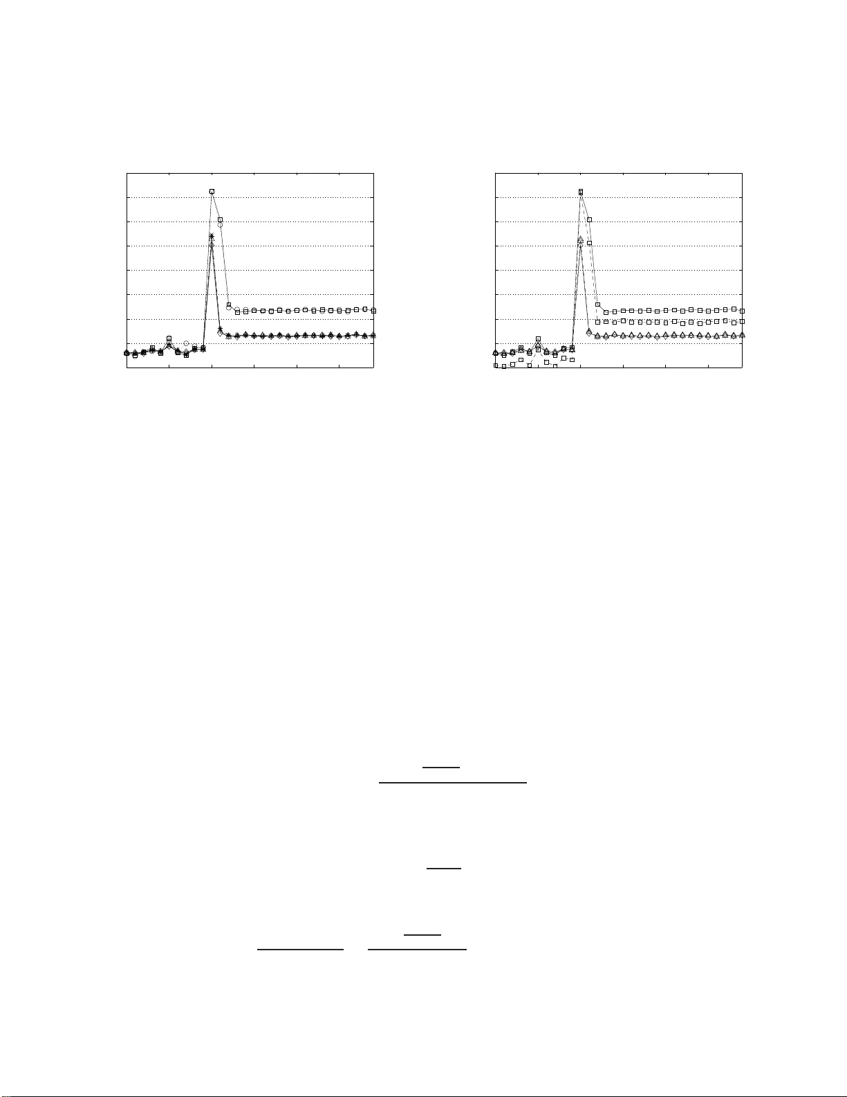
AD APTIVE METHODS F OR SEQUENTIA L IMP OR T ANCE SAMPLING WITH APP LICA TION TO ST A TE SP A CE MODELS JULIEN CORNEBISE, ´ ERIC MOULINES, AND JIMMY O LSSON Abstract. In this paper we discuss new adaptive prop osal s trategies for seq uen tial Mo n te Carlo algo rithms—also known as par ticle ﬁlters—re ly ing on cr iteria ev aluating the quality of the prop osed pa r ticles. The choice of the prop osal distribution is a ma jor concern and can dr amatically inﬂuence the quality of the estimates. Th us, we show how the lo ng -used co eﬃcient of v ariation (sugges ted by Kong et al. ( 1994 )) of the weigh ts can be used for estimating the chi-square dista nc e betw een the ta rget and instrumental dis tributions of the auxiliary particle ﬁlter . As a by-product o f this ana lysis we obtain a n auxiliary a djustmen t m ultiplier weight t yp e for which this chi-square distance is minimal. Mo reov er, we establish an empirical estimate o f linea r complexity of the Kullback-Leibler divergence betw een the inv olv ed distributions. Guided by these results, w e discuss adaptive designing of the particle ﬁlter pro po sal dis tr ibution and illustrate the methods on a numerical exa mple. 1. Introduction Easing the role of the user b y tuning a utomatically the k ey pa rameters of se quential Monte Carlo (SMC) algorithms has b een a long-standing to pic in the communit y , notably throug h adaptation of the pa rticle sample size or the w ay the particles are sampled and we igh ted. In t his pap er w e fo cus on the latter issue and dev elop metho ds for adjusting ada ptiv ely the prop osal distribution of the part icle ﬁlter. Adaptation o f the n umber of par t icles has b een treated by sev eral author s. In Legland and Oudjane ( 2006 ) (and later Hu et al. ( 200 8 , Section IV)) the size of the particle sample is increased until the total we igh t mass reac hes a p ositive threshold, a voiding a situation where all particles are lo cated in regions of the state space ha ving zero p osterior probability . F earnhead a nd Liu ( 2 0 07 , Section 3.2) adjust the size of the par t icle cloud in order to con trol the erro r in tro duced by the resampling step. Another approach, suggested b y F ox ( 2003 ) and reﬁned in Soto ( 2005 ) and Strak a and Simandl ( 2006 ), consists in increasing t he sample size un til the Kul lb ack-L eibler diver genc e (KLD) b et we en the true and estimated target distributions is b elo w a given threshold. Date : July 2008 . 2000 Mathematics Subje ct Classiﬁc ation. Primary 65C05 ; Se c o ndary 60 G35. Key wor ds and phr ases. Adaptive Mon te Carlo, Auxiliar y particle ﬁlter, Co eﬃcient of v a riation, Kullback- Leibler divergence, Cro ss-entropy method, Sequential Monte Carlo , Sta te s pace mo dels. This w ork was partly supp orted by the Natio nal Research Agency (ANR) under the pr ogra m “ ANR-05- BLAN-0299 ” . 1 2 J. CORN EBISE, ´ E. MOULI NES, AN D J. OLSSO N Unarguably , setting an appropriate sample size is a k ey ingredien t of a n y statistical esti- mation pro cedure, and there are cases where the metho ds mentioned ab o v e may b e used for designing satisfactorily this size; how ev er increasing the sample size only is far from b eing alw ays suﬃcien t for ac hieving eﬃcien t v a r ia nce reduction. Indeed, a s in a n y algorithm based on imp o rtance sampling, a signiﬁcan t discrepancy b etw een the prop osal and targ et distri- butions may require an unreasonably large n um b er o f samples for decreasing the v aria nce of the estimate under a sp eciﬁed v alue. F or a ve ry simple illustration, consider imp ortance sampling estimation of the mean m o f a normal distribution using a s imp o rtance distribution another normal distribution ha ving zero mean and same v a riance: in this case, the v a riance of the estimate grows like exp( m 2 ) / N , N denoting the n umber o f draws , implying tha t the sample size r equired f or ensuring a giv en v ariance grows exp onen t ia lly fast with m . This p oints to t he need for adapting the imp ort a nce distribution of the particle ﬁlter, e.g., b y adjusting at eac h iteration the particle we igh ts and the prop osal distributions; see e.g. Doucet et a l. ( 2 0 00 ), Liu ( 2004 ), and F earnhead ( 2008 ) for reviews of v arious ﬁltering metho ds. These tw o quan tities are critically imp ortant, since the p erformance of the particle ﬁlter is closely related to the abilit y of prop osing particles in state space r egio ns where the p osterior is signiﬁcan t. It is well know n that sampling using as prop osal distribution the mixture comp osed by the curren t particle imp o rtance w eights and the prior kernel (yielding the classical b o o t strap particle ﬁlter of Gordon et al. ( 1993 )) is usually ineﬃcien t when the lik eliho o d is hig hly p eak ed or lo cated in the tail of the pr io r. In the sequen tial con text, the succes siv e distributions to b e appro ximated (e.g. t he succes- siv e ﬁltering distributions) are t he iterates of a nonlinear random mapping, deﬁned o n the space of probability measures; this nonlinear mapping ma y in general b e decomp osed into t wo steps: a prediction step whic h is linear a nd a nonlinear correction step whic h amounts to compute a normalisation fa cto r . In this setting, an app ealing wa y to up date the curren t particle approximation consists in sampling new particles fr om the distribution obtained by propagating the current par t icle approximation throug h this mapping; see e.g. H ¨ urzeler and K ¨ unsc h ( 1998 ), Doucet et al. ( 2000 ), and K ¨ unsc h ( 2005 ) (and the references therein). This sampling distribution g uaran tees that the conditional v ariance of the imp ortance w eights is equal to zero. As we shall see b elo w, this pro p osal distribution enjoy s o t her optimality conditions, a nd is in the sequel referred to a s the op timal sampling distribution . Ho wev er, sampling from the o pt imal sampling distribution is, except for some sp eciﬁc mo dels, a dif- ﬁcult and time-consuming task (the in general costly auxiliary accept-reject dev elop ed a nd analysed b y K ¨ unsc h ( 200 5 ) b eing most of ten the only a v ailable option). T o circum v en t this diﬃculty , sev era l sub-optimal sc hemes hav e b een pro p osed. A ﬁrst t yp e o f approaches tries to mimic the b eha vior of the optimal sampling without suﬀering the sometimes prohibitiv e cost of rejection sampling. This t ypically inv olv es lo calisation of the mo des of the unnormalised optimal sampling distribution b y means of some optimisation algorithm, and the ﬁtting of ov er-disp ersed student’s t - distributions around these mo des; see for example Shephard and Pitt ( 1 997 ), Doucet et al. ( 2001 ), and Liu ( 200 4 ) (a nd the r efer- ences therein). Except in sp eciﬁc cases, lo cating the mo des inv olve s solving an optimisation problem f o r ev ery particle, whic h is quite t ime-consuming. ADAPTIVE METHODS FOR S EQ U ENTIAL I MPOR T AN CE SAMPLING 3 A second class of approaches consists in using some classical approx imate non-linear ﬁl- tering to o ls suc h as the extende d Kalman ﬁlter (EKF ) or the unsc ente d tr ansform Kalman ﬁlter (UT/UKF); see for example Doucet et al. ( 2001 ) and the references therein. These tec hniques assume implicitly that the conditional distribution of the next state give n the curren t state and the observ at io n has a single mo de. In the EKF v ersion of the particle ﬁlter, t he linearisation of the state and o bserv ation equations is carried out f o r each indi- vidual par t icle. Instead of linearising the state and observ a t io n dynamics using Jacobia n matrices, t he UT/UKF particle ﬁlter uses a deterministic sampling strategy to capture the mean and co v ariance with a small set o f carefully selected p oin ts ( sigma p oints ), whic h is also computed fo r eac h particle. Since these computations a r e most often rather in volv ed, a signiﬁcan t computat io nal o verhe ad is in t r o duced. A third class of tec hniques is the so-called auxiliary p article ﬁl ter (APF) suggested by Pitt and Shephard ( 1999 ), who prop osed it as a wa y to build data-driven prop osal distributions (with the initial aim of robustifying standard SMC metho ds to the presence of outlying observ ations); see e.g. F earnhead ( 2008 ). The pro cedure comprises t wo stages: in the ﬁrst- stage, t he curren t part icle w eights are mo diﬁed in order to select preferen tially those particles b eing most lik ely prop osed in regions where the p osterior is signiﬁcant. Usually this amounts to m ultiply the w eights with so-called a d justment multiplier weights , which ma y dep end on the next observ a tion as w ell as the current p osition of the particle and (p ossibly) the pro p osal transition kernels . Most often, this adjustment w eight is c hosen to estimate the predictiv e lik eliho o d of the next observ atio n given the curren t particle p osition, but this c ho ice is not necessarily optimal. In a second stage, a new part icle sample from the target distribution is formed using this prop osal distribution and asso ciating the prop osed particles with weigh t s prop ortiona l to the in vers e of the adjustmen t mu ltiplier weigh t 1 . APF pro cedures are kno wn to b e ra ther success ful when the ﬁrst-stage distribution is appropriately chos en, whic h is not alw ay s straigh tf orw ard. The additional computatio nal cost dep ends mainly on the wa y the ﬁr st- stage prop osal is designed. The APF metho d can b e mixed with EKF and UKF leading to p ow erful but computationally inv olved particle ﬁlter; see, e.g., Andrieu et al. ( 200 3 ). None of the sub optimal methods men tioned ab o v e minimise an y sensible risk-theoretic criterion and, more anno yingly , b o t h theoretical and practical evidences sho w that c hoices whic h seem to b e intuitiv ely correct ma y lead to p erformances ev en w orse than that of the plain b o otstrap ﬁlter (see for example D ouc et al. ( 2008 ) fo r a striking example). The situation is ev en more unsatisfactory when the particle ﬁlter is driven by a state space dynamic diﬀeren t from that generating the observ ations, as happ ens frequen tly when, e.g., the pa r a meters are not know n and need to b e estimated or when the mo del is missp eciﬁed. Instead of trying to guess what a go o d prop osal distribution should b e, it seems sensible to follo w a more r isk-theoretically founded approac h. The ﬁrst step in suc h a construction 1 The orig inal APF prop osed by Pitt a nd Shephard ( 1999 ) features a se cond res ampling pro cedure in orde r to end-up with an equally weigh ted par ticle sy s tem. T his resampling pro cedure might ho wever severely reduce the a ccuracy of the ﬁlter : Carp enter et al. ( 1 999 ) give an ex a mple where the accura cy is reduced by a facto r of 2; see also Douc et al. ( 2 008 ) for a theoretical pro of. 4 J. CORN EBISE, ´ E. MOULI NES, AN D J. OLSSO N consists in c ho osing a sensible risk criterion, whic h is not a straig h tfo r w ard task in the SMC con text. A natural criterion for SMC w ould b e the v ariance of the estimate of the p osterior mean of a t arget function (or a set of target functions) of inte rest, but this approa c h do es not lead to a pra ctical implemen tatio n for tw o reasons. Firstly , in SMC metho ds, though closed-form expression f o r the v ariance at an y giv en curren t time-step of the p osterior mean of an y function is a v ailable, this v ariance dep ends explicitly on all the time steps b efore the curren t time. Hence, choosing to minimise the v ariance at a giv en time-step w ould require to optimise all the sim ulations up to t hat part icular time step, whic h is of course not practical. Because of the recursiv e f orm of the v ariance, the minimisation of the conditional v ariance at eac h itera t io n of the a lgorithm do es not necessarily lead to satisfactory p erformance on the long-run. Secondly , as for the standard imp ortance sampling algorithm, t his criterion is not function-fr e e , meaning tha t a c hoice of a prop osal can b e appropriate for a give n function, but inappropriate for a no ther. W e will fo cus in the sequel on function-free risk criteria. A ﬁrst criterion, a dv o cat ed in Kong et a l. ( 199 4 ) and Liu ( 2004 ) is the chi-squar e dis tan c e (CSD) b et w een the prop osal and the target distributions, whic h coincides with the c o eﬃ c ient of variation (CV 2 ) of t he imp ortance weigh t s. In addition, as heuristically discussed in Kong et al. ( 1994 ), the CSD is related t o the e ﬀ e ctive sample size , whic h estimates t he n umber o f i.i.d. samples equiv alen t to the we igh ted pa r t icle system 2 . In practice, the CSD criterion can b e estimated, with a complexit y that grows linearly with the n umber of particles, using the empirical CV 2 whic h can b e sho wn to con v erge to the CSD as the num b er o f particles tends to inﬁnity . In this pap er w e show that a similar prop erty still holds in t he SMC contex t, in the sense that the CV 2 still measures a CSD b etw een tw o distributions µ ∗ and π ∗ , whic h are asso ciated with the pro p osal and tar g et distributions of the particle ﬁlter (see Theorem 4.1 (ii)). Though this result do es not come as a surprise, it prov ides an additional theoretical fo oting to an approac h whic h is curren tly used in practice for triggering resampling steps. Another function-f ree risk criterion to a ssess the p erformance of imp ortance sampling estimators is the K L D b et we en the prop osal and the target distributions; see ( Capp ´ e et al. , 2005 , Chapter 7) . The KLD shares some of the attractive pr o p erties of the CSD; in particular, the KL D may b e estimated using the negated empirical entr op y E of the imp ortance w eigh ts, whose computationa l complexit y is again linear in the num b er of particles. In the SMC con text, it is shown in Theorem 4.1 (i) that E still conv erges to the KL D b etw een the same t wo distributions µ ∗ and π ∗ asso ciated with the prop osal and the tar get distributions of the particle ﬁlter. Our metho do lo gy to design appropriate prop o sal distributions is based up on the minimi- sation of the CSD and KLD b etw een the prop osal a nd the target distributions. Whereas these quantities ( a nd esp ecially the CSD) hav e b een routinely used to detect sample imp ov - erishmen t and trigger the resampling step ( Kong et a l. , 1994 ), they hav e not b een used fo r adapting the sim ulation para meters in SMC metho ds. 2 In some situations, the e s timated ESS v alue ca n b e misleading: see the co mmen ts of Stephens and Donnelly ( 2000 ) for a fur ther discussion o f this. ADAPTIVE METHODS FOR S EQ U ENTIAL I MPOR T AN CE SAMPLING 5 W e fo cus here on the auxiliary sampling form ula tion of the part icle ﬁlter. In this setting, there are tw o quan tities to optimise: the adjustmen t m ultiplier weigh ts (also called ﬁrs t- stage weights ) and the parameters o f the prop osal ke rnel; together these quan t it es deﬁne the mixture used as instrumen tal distribution in the ﬁlter. W e ﬁrst establish a closed- form expression for the limiting v alue of the CSD and KLD o f t he auxiliary formulation of the prop osal and the targ et distributions. Using these expres sions, w e iden tify a ty p e of auxiliary SMC adjustmen t m ultiplier we igh t s which minimise the CSD and t he KLD for a giv en prop osal k ernel (Prop osition 4.2 ). W e then prop ose sev eral optimisation tec hniques for ada pting the prop osal k ernels, alw ays driven by the ob jectiv e of minimising the CSD or the KLD , in coherence with what is done to detect sample imp o veris hmen t (see Section 5 ). Finally , in the implemen tat io n section (Section 6 ), w e use the prop o sed algorithms for appro ximating the ﬁltering distributions in sev eral state space mo dels, and sho w that the prop osed optimisation pro cedure improv es the accuracy of t he par t icle estimates and mak es them more robust to outlying observ ations. 2. Inf ormal prese nt a tion of the res ul ts 2.1. Adaptive imp or t ance sampling. Before stating and pro ving rigorously the main results, w e discuss informally our ﬁndings a nd introduce the prop osed metho dology for de- v eloping a da ptiv e SMC algorithms. Before en tering into the sophistication of sequen tial metho ds, w e ﬁrst brieﬂy in tro duce adaptation of the standard (non-sequen tial) imp ortance sampling a lgorithm. Imp ortanc e sampling (IS) is a general tec hnique to compute exp ectations of functions with resp ect to a ta r get distribution with densit y p ( x ) while only having samples generated from a diﬀeren t distribution—referred to as the pr op osal distribution — with densit y q ( x ) (implicitly , the dominating measure is taken to b e the Leb esgue measure on Ξ , R d ). W e sample { ξ i } N i =1 from the prop osal distribution q and compute the unnormalised imp ortance w eights ω i , W ( ξ i ), i = 1 , . . . , N , where W ( x ) , p ( x ) /q ( x ). F or any function f , the self- normalised imp ortance sampling estimator may b e expressed as IS N ( f ) , Ω − 1 N P N i =1 ω i f ( ξ i ), where Ω N , P N j =1 ω j . As usual in applications of the IS metho dology to Bay esian inference, the ta rget densit y p is kno wn only up to a normalisation constan t; hence w e will fo cus only on a self-normalised v ersion of IS that solely requires the av aila bility of a n unnor malised v ersion of p (see Gew ek e , 198 9 ). Througho ut the pap er, we call a set { ξ i } N i =1 of random v ariables, referred to as p articles and taking v alues in Ξ , and nonnegativ e w eights { ω i } N i =1 a weighte d sa mple on Ξ . Here N is a (p ossibly random) in teger, though w e will take it ﬁxed in the sequel. It is w ell kno wn (see aga in Gew ek e , 1989 ) that, pro vided that f is integrable with resp ect to p , i.e. R | f ( x ) | p ( x ) d x < ∞ , IS N ( f ) conv erges, as the num b er of samples tends to inﬁnit y , to the ta r g et v alue E p [ f ( X )] , Z f ( x ) p ( x ) d x , 6 J. CORN EBISE, ´ E. MOULI NES, AN D J. OLSSO N for an y function f ∈ C , where C is t he set of functions whic h are in tegrable with resp ect to to the targ et distribution p . Under some additional tec hnical conditions, th is estimator is also asymptotically normal at ra t e √ N ; see G ew ek e ( 1989 ). It is we ll kno wn that IS estimators are sensitiv e to the choice of the prop osal distribution. A classical approac h consists in trying to minimise the asymptotic v aria nce with respect to the prop osal distribution q . This optimisation is in closed form and leads (when f is a non-negativ e function) to t he opt ima l c hoice q ∗ ( x ) = f ( x ) p ( x ) / R f ( x ) p ( x ) d x , which is, since the normalisation constant is precisely the quantit y of interes t, r a ther impractical. Sampling from this distribution can b e done b y using a n accept-reject algorithm, but this do es not solv e the problem of choosing an appropriate prop osal distribution. Note that it is p ossible to approa c h t his optimal sampling distribution b y using the cr oss-entr opy metho d ; see Rubinstein and Kro ese ( 2004 ) and de Bo er et al. ( 2005 ) and the references therein. W e will discuss this p oint later on. F or reasons that will b ecome clear in the sequel, this type of ob jectiv e is impractical in the sequen t ia l con text, since the express ion of t he asymptotic v ariance in this case is recursiv e and the optimisation of the v ariance at a giv en step is impo ssible. In addition, in most applications, the pro p osal density is exp ected to p erform w ell fo r a range of t ypical functions of in terest rather t han for a sp eciﬁc target function f . W e are th us lo oking for function-fr e e criteria. The most often used criterion is the CSD b et wee n the prop osal distribution q and the ta rget distribution p , deﬁned as d χ 2 ( p || q ) = Z { p ( x ) − q ( x ) } 2 q ( x ) d x , (2.1) = Z W 2 ( x ) q ( x ) d x − 1 , (2.2) = Z W ( x ) p ( x ) d x − 1 . (2.3) The CSD b et we en p and q may b e expressed as the v ariance of the imp or t ance weigh t function W under the prop osal distribution, i.e. d χ 2 ( p || q ) = V ar q [ W ( X )] . This quan tity can b e estimated b y computing the squared coeﬃcien t o f v ariation of the unnormalized w eights ( Ev ans and Sw artz , 1995 , Section 4 ) : CV 2  { ω i } N i =1  , N Ω − 2 N N X i =1 ω 2 i − 1 . (2.4) The CV 2 w as suggested by Kong et a l. ( 1 9 94 ) as a means fo r detecting weigh t degeneracy . If all the w eights are equal, then CV 2 is equal to zero. On the other hand, if all the we igh ts but one ar e zero, then the co eﬃcien t of v ariat io n is equal to N − 1 whic h is its maxim um v alue. F rom this it follows that using the estimated co eﬃcien t of v a r ia tion for assess ing accuracy is equiv alen t to examining the norma lised imp ortance weigh ts to determine if an y ADAPTIVE METHODS FOR S EQ U ENTIAL I MPOR T AN CE SAMPLING 7 are relativ ely large 3 . Kong et al. ( 1994 ) sho wed that the co eﬃcien t of v ariation of the we igh ts CV 2 ( { ω i } N i =1 ) is related to the eﬀe ctive samp le s i z e (ESS), whic h is used f or measuring the o verall eﬃciency of an IS alg orithm: N − 1 ESS  { ω i } N i =1  , 1 1 + CV 2  { ω i } N i =1  → { 1 + d χ 2 ( p || q ) } − 1 . Heuristically , the ESS measures the n umber of i.i.d. samples (from p ) equiv alen t to the N w eighte d samples. The smaller the CSD b etw een the prop osal and ta rget distributions is, the larger is the ESS. This is wh y the CSD is of particular interes t when measuring eﬃciency of IS algor ithms. Another p ossible measure of ﬁt o f the prop o sal distribution is the KLD (also called r elative entr opy ) b et wee n the prop osal and target distributions, deﬁned as d KL ( p || q ) , Z p ( x ) log  p ( x ) q ( x )  d x , (2.5) = Z p ( x ) log W ( x ) d x , (2.6) = Z W ( x ) log W ( x ) q ( x ) d x . (2.7) This criterion can b e estimated from the imp ortance weigh ts using the negative Shann on entr opy E o f the imp orta nce w eights : E  { ω i } N i =1  , Ω − 1 N N X i =1 ω i log  N Ω − 1 N ω i  . (2.8) The Shannon en tropy is maximal when all the w eigh ts a re equal and minimal when all w eights are zero but one. In IS (and esp ecially for the estimation of rare eve n ts), the KLD b et ween t he prop osal and target distributions w as tho r oughly inv estigated b y Rubinstein and Kro ese ( 2004 ), and is cen tra l in the cr oss-entr opy ( CE) metho do logy . Classically , the pro p osal is chosen f rom a family of densities q θ parameterised b y θ . Here θ should b e thought of as a n elemen t of Θ, whic h is a subset of R k . The most classical example is the family o f student’s t - distributions parameterised by mean a nd co v ariance. More sophisticated para meterisations, lik e mixture of multi-dimensional Gaussian or Stu- den t’s t -distributions, ha v e b een pr o p osed; see, e.g., Oh a nd Berger ( 1992 ), O h and Berger ( 1993 ), Ev ans and Sw artz ( 1995 ), G iv ens and R aftery ( 1996 ), Liu ( 2004 , Chapter 2, Section 2.6), and, more recently , Capp ´ e et a l. ( 2008 ) in this issue. In the sequen t ia l context, where computational eﬃciency is a must, w e typic ally use ra ther simple parameterisations, so that the tw o criteria ab ov e can b e (approx imativ ely) solve d in a few iterations of a nume rical minimisation pro cedure. 3 Some care sho uld b e taken for sma ll sample sizes N ; the CV 2 can b e low b e cause q sa mple only ov er a subregion wher e the integrand is nea rly co nstant, which is not always easy to detect. 8 J. CORN EBISE, ´ E. MOULI NES, AN D J. OLSSO N The opt ima l parameters for the CSD and the KLD are those minimising θ 7→ d χ 2 ( p || q θ ) and θ 7→ d KL ( p || q θ ), resp ectiv ely . In the sequel, w e denote by θ ∗ CSD and θ ∗ KLD these optima l v alues. Of course, these quan tities cannot be computed in closed form (recall that ev en the normalisation constan t of p is most often unknow n; ev en if it is know n, the ev aluation of these quan tities would in v olve the ev aluation of most often high-dimensional integrals). Nev ertheless, it is p o ssible to construct consisten t estimators of these optimal parameters. There are tw o classes of metho ds, detailed b elow. The ﬁrst uses the fa ct that the the CSD d χ 2 ( p || q θ ) and the KLD d KL ( p | q θ ) ma y b e ap- pro ximated b y ( 2.4 ) and ( 2.8 ), substituting in these expressions the imp ortance w eights b y ω i = W θ ( ξ θ i ), i = 1 , . . . , N , where W θ , p /q θ and { ξ θ i } N i =1 is a sample from q θ . This optimi- sation problem formally shares some similarities with the classical minim um chi-square or maxim um lik eliho o d estimation, but with the following imp ortant diﬀerence: the integra- tions in ( 2.1 ) and ( 2.5 ) are with resp ect to the prop osal distribution q θ and not the target distribution p . As a consequence, the particles { ξ θ i } N i =1 in the deﬁnition of the co eﬃcien t of v ariat io n ( 2.4 ) or the en trop y ( 2.8 ) of the we igh t s constitute a sample from q θ and not fr om the target distribution p . As the estimation progr esses, the samples used to a pproac h the limiting CSD or K L D can, in contrast to standard estimation pro cedures, b e up dated (these samples could b e kept ﬁxed, but this is o f course ineﬃcien t). The computational complexit y of these optimisation problems dep ends on the w ay the prop osal is parameterised a nd how the optimisation pro cedure is implemen ted. Though the details of the optimisation pro cedure is in general strongly mo del dep enden t, some common principles for solving t his o ptimisatio n problem can b e outlined. T ypically , the optimisation is done recursiv ely , i.e. the algorithm deﬁnes a sequence θ ℓ , ℓ = 0 , 1 , . . . , of parameters, where ℓ is the iteration n umber. A t eac h iteration, the v a lue of θ ℓ is up dated b y computing a direction p ℓ +1 in whic h to step, a step length γ ℓ +1 , and setting θ ℓ +1 = θ ℓ + γ ℓ +1 p ℓ +1 . The search direction is t ypically computed using either Mon te Carlo appro ximation of the ﬁnite-diﬀerence o r (when the quan tities of in terest ar e suﬃcien tly regular) the gradien t o f the criterion. These quan tities are used la t er in conjunction with classical optimisation strategies for computing the step size γ ℓ +1 or normalising the search direction. These implemen tation issues, detailed in Section 6 , are mo del dep enden t. W e denote by M ℓ the n umber of particles used to obtain suc h a n approx imation at iterat io n ℓ . The n um b er of particles ma y v ary with the iteration index; heuristically there is no need for using a large num b er o f sim ulations during the initial stage of the optimisation. Ev en rat her crude estimation of the searc h direction migh t suﬃce to drive the para meters to wards the region of in terest. How ev er, as the iterations g o on, the n umber of simulations should b e increased to a v oid “zi g-zagging” when the a lg orithm approa c hes con ve rgence. After L iteratio ns, the total n umber of generated particles is equal to N = P L ℓ =1 M ℓ . Another solution, whic h is not considered in t his pap er, w ould b e to use a sto c hastic approximation pro cedure, whic h consists in ﬁxing M ℓ = M and letting the stepsize γ ℓ tend to zero. This app ealing solution has b een successfully used in Arouna ( 2004 ). ADAPTIVE METHODS FOR S EQ U ENTIAL I MPOR T AN CE SAMPLING 9 The computation of the ﬁnite diﬀerence or the gradient, b eing deﬁned as exp ectations of functions dep ending on θ , can b e p erformed using tw o diﬀeren t approac hes. Starting f rom deﬁnitions ( 2.3 ) and ( 2.6 ), and a ssuming appro priate regularity conditions, the g radien t of θ 7→ d χ 2 ( p || q θ ) and θ 7→ d KL ( p || q θ ) ma y b e expressed as G CSD ( θ ) , ∇ θ d χ 2 ( p || q θ ) = Z p ( x ) ∇ θ W θ ( x ) d x = Z q θ ( x ) W θ ( x ) ∇ θ W θ ( x ) d x , (2.9) G KLD ( θ ) , ∇ θ d KL ( p || q θ ) = Z p ( x ) ∇ θ log[ W θ ( x )] d x = Z q θ ( x ) ∇ θ W θ ( x ) d x . (2.10) These expressions lead immediately to the follow ing appro ximations, ˆ G CSD ( θ ) = M − 1 M X i =1 W θ ( ξ θ i ) ∇ θ W θ ( ξ θ i ) , (2.11) ˆ G KLD ( θ ) = M − 1 M X i =1 ∇ θ W θ ℓ ( ξ θ ℓ i ) . (2.12) There is another wa y to compute deriv ativ es, whic h shares some similarities with p athwise derivative estima tes . Recall tha t for any θ ∈ Θ, one ma y c ho ose F θ so t ha t the random v ariable F θ ( ǫ ), where ǫ is a v ector of independent uniform random v ariables on [0 , 1] d , is distributed according to q θ . Therefore, w e may express θ 7→ d χ 2 ( p || q θ ) a nd θ 7→ d KL ( p || q θ ) as t he fo llo wing integrals, d χ 2 ( p || q θ ) = Z [0 , 1] d w θ ( x ) d x , d KL ( p || q θ ) = Z [0 , 1] d w θ ( x ) log [ w θ ( x )] d x , where w θ ( x ) , W θ ◦ F θ ( x ). Assuming appropriate regularity conditions (i.e. that θ 7→ W θ ◦ F θ ( x ) is diﬀeren tia ble and that w e can in terchange the in tegra tion and t he diﬀeren tiation), the diﬀerential o f these quan tities with resp ect to θ may b e expressed as G CSD ( θ ) = Z [0 , 1] d ∇ θ w θ ( x ) d x , G KLD ( θ ) = Z [0 , 1] d {∇ θ w θ ( x ) log [ w θ ( x )] + ∇ θ w θ ( x ) } d x . F or any giv en x , the quan tit y ∇ θ w θ ( x ) is the pathw ise deriv at ive of the function θ 7→ w θ ( x ). As a practical matter, w e usually t hink of each x as a realizatio n of of the output o f an ideal random generator. Eac h w θ ( x ) is then the output of the simulation algorit hm at parameter θ for the random num b er x . Eac h ∇ θ w θ ( x ) is the deriv ativ e of the sim ula tion o utput with resp ect to θ with the random num b ers held ﬁxed. These tw o expressions , whic h o f course 10 J. CORN EBISE, ´ E. MOULI NES, AN D J. OLSSO N coincide with ( 2 .9 ) and ( 2.10 ), lead to the f ollo wing estimators, ˜ G CSD ( θ ) = M − 1 M X i =1 ∇ θ w θ ( ǫ i ) , ˜ G KLD ( θ ) = M − 1 M X i =1 {∇ θ w θ ( ǫ i ) log [ w θ ( ǫ i )] + ∇ θ w θ ( ǫ i ) } , where eac h elemen t of the sequence { ǫ i } M i =1 is a v ector on [0 , 1] d of independen t unifor m random v ariables. It is w orthwhile t o no te that if the num b er M ℓ = M is k ept ﬁxed during the iterations and the uniforms { ǫ i } M i =1 are dra wn once and for all (i.e. the same uniforms are used at the diﬀeren t iterations), t hen the iterativ e algo r it hm outlined ab ov e solves the follo wing problem: θ 7→ CV 2  { w θ ( ǫ i ) } M i =1  , (2.13) θ 7→ E  { w θ ( ǫ i ) } N i =1  . (2.14) F rom a theoretical standp oin t, this optimisation problem is v ery similar to M -estimation, and con v ergence results for M -estimators can th us b e used under ra t her standard tec hnical assumptions; see f o r example V an der V aart ( 1998 ). This is the main adv an ta ge of ﬁxing the sample { ǫ i } M i =1 . W e use this implemen tation in the sim ulations. Under appropriate conditions, t he sequence of estimators θ ∗ ℓ, CSD or θ ∗ ℓ, KLD of these criteria con ve rge, as the num b er of iterat io ns tends to inﬁnity , t o θ ∗ CSD or θ ∗ KLD whic h minimise the criteria θ 7→ d χ 2 ( p || q θ ) and θ 7→ d KL ( p || q θ ), resp ectiv ely; t hese theoretical issue s are considered in a companion pap er. The second class o f a pproac hes considered in this pap er is used for minimising the KLD ( 2.14 ) and is inspired by the cro ss-entrop y metho d. This algorithm approximates the min- im um θ ∗ KLD of ( 2.14 ) b y a sequence of pairs of steps, where eac h step o f eac h pair ad- dresses a simpler optimisation problem. Compared to the previous metho d, this algorithm is deriv ative -free and do es not require to select a step size. It is in general simpler to implemen t and av oid most of the common pitf alls of sto chastic approx imation. Denote by θ 0 ∈ Θ an initial v alue. W e deﬁne recursiv ely the sequence { θ ℓ } ℓ ≥ 0 as follows . In a ﬁrst step, w e dra w a sample { ξ θ ℓ i } M ℓ i =1 and ev aluate the function θ 7→ Q ℓ ( θ , θ ℓ ) , M ℓ X i =1 W θ ℓ ( ξ θ ℓ i ) log q θ ( ξ θ ℓ i ) . (2.15) In a second step, w e c ho ose θ ℓ +1 to b e the (or a n y , if there are sev eral) v alue of θ ∈ Θ that maximises Q ℓ ( θ , θ ℓ ). As ab ov e, the num b er of particles M ℓ is increased during the successiv e iterations. This pro cedure ressem bles closely the Monte Carlo EM ( W ei and T anner , 1991 ) for maximum lik eliho o d in incomplete data mo dels. The adv an tage o f this approac h is that the solution of the maximisation pro blem θ ℓ +1 = argmax θ ∈ Θ ∈ Q ℓ ( θ , θ ℓ ) is often on closed form. In particular, this happ ens if the distribution q θ b elongs to a n exp on ential f a mily ADAPTIVE METHODS FOR S EQ U ENTIAL I MPOR T AN CE SAMPLING 11 (EF) or is a mixture of distributions of NEF; see Capp ´ e et al. ( 2 008 ) fo r a discussion. The con ve rgence of this algorithm can b e established along the same lines as the conv erg ence of the MCEM algor ithm; see F ort and Moulines ( 2003 ) . As the n um b er o f iterations ℓ increases, the sequence of estimators θ ℓ ma y b e shown to con v erge to θ ∗ KLD . These theoretical results are established in a companion pap er. 2.2. Sequen t ial Mon te Carlo Metho ds. In the sequen tial con text, where the problem consists in simulating from a se quenc e { p k } of probability densit y function, the situation is more diﬃcult. Let Ξ k b e denote the state space of distribution p k and note that this space ma y v ary with k , e.g. in terms of increasing dimensionalit y . In many applications, these densities are r elat ed to eac h other by a (p ossibly random) mapping, i.e. p k = Ψ k − 1 ( p k − 1 ). In the sequel we fo cus o n the case where there exists a non-negativ e function l k − 1 : ( ξ , ˜ ξ ) 7→ l k − 1 ( ξ , ˜ ξ ) suc h that p k ( ˜ ξ ) = R l k − 1 ( ξ , ˜ ξ ) p k − 1 ( ξ ) d ξ R p k − 1 ( ξ ) R l k − 1 ( ξ , ˜ ξ ) d ˜ ξ d ξ . (2.16) As an example, consider the fo llo wing generic nonlinear dynamic system describ ed in stat e space form: • State (system) mo del X k = a ( X k − 1 , U k ) ↔ T ransition Densit y z }| { q ( X k − 1 , X k ) , (2.17) • Observation (me asur ement) m o d e l Y k = b ( X k , V k ) ↔ Observ ation Densit y z }| { g ( X k , Y k ) . (2.18) By these equations we mean that eac h hidden state X k and data Y k are assumed t o b e generated b y nonlinear functions a ( · ) a nd b ( · ), resp ectiv ely , of t he state and observ ation noises U k and V k . The state a nd the observ ation noises { U k } k ≥ 0 and { V k } k ≥ 0 are assumed to b e m utually indep enden t sequence s of i.i.d. random v ariables. The precise form of the functions and the assumed probabilit y distributions of the state and observ atio n noises U k and V k imply , via a c hange of v ariables, the tr ansition probability densit y function q ( x k − 1 , x k ) and the observ ation probabilit y densit y function g ( x k , y k ), the lat t er b eing referred to as the likeliho o d of the observation . With these deﬁnitions, the pro cess { X k } k ≥ 0 is Mark ovian, i.e. the conditional probability densit y of X k giv en the past states X 0: k − 1 , ( X 0 , . . . , X k − 1 ) dep ends exclusiv ely on X k − 1 . This distribution is described b y t he densit y q ( x k − 1 , x k ). In addition, the conditional probability densit y of Y k giv en the states X 0: k and the past observ ations Y 0: k − 1 dep ends exclusiv ely on X k , and this distribution is captured b y the lik eliho o d g ( x k , y k ). W e assume further that the initia l state X 0 is distributed according to a density function π 0 ( x 0 ). Suc h nonlinear dynamic syste ms arise frequen tly in man y areas of science and engineering suc h as t a rget tra c king, computer vision, terrain referenced 12 J. CORN EBISE, ´ E. MOULI NES, AN D J. OLSSO N na vigatio n, ﬁnance, p ollution monitoring, comm unications, audio engineering, to list only a few. Statistical inference for the general nonlinear dynamic system ab ov e inv olves computing the p osterior distribution of a collection of state v ariables X s : s ′ , ( X s , . . . , X s ′ ) conditioned on a batc h Y 0: k = ( Y 0 , . . . , Y k ) o f observ ations. W e denote this p osterior distribution by φ s : s ′ | k ( X s : s ′ | Y 0: k ). Sp eciﬁc problems include ﬁltering , corr espo nding to s = s ′ = k , ﬁxe d lag smo othing , where s = s ′ = k − L , and ﬁxe d interval smo othing , with s = 0 and s ′ = k . Despite the apparen t simplicity of the a b o v e problem, t he p osterior distributions can b e computed in closed form only in v ery sp eciﬁc cases, principally , the linear Ga ussian mo del (where the functions a ( · ) a nd b ( · ) are linear and the state and observ at ion noises { U k } k ≥ 0 and { V k } k ≥ 0 are G aussian) and the discrete hid d en Markov mo del (where X k tak es its v alues in a ﬁnite alphab et). In the v ast ma jorit y of cases, no nlinearity or non-Gaussianity render analytic solutions intractable—see Anderson and Mo ore ( 1979 ); Ka ilath et al. ( 20 00 ); Ristic et a l. ( 2004 ); Capp ´ e et al. ( 2 0 05 ). Starting with t he initial, or prio r, densit y function π 0 ( x 0 ), and observ ations Y 0: k = y 0: k , the p osterior densit y φ k | k ( x k | y 0: k ) can b e obtained using the following pr e diction - c orr e ction recursion ( Ho and Lee , 1964 ): • Pr e diction φ k | k − 1 ( x k | y 0: k − 1 ) = φ k − 1 | k − 1 ( x k − 1 | y 0: k − 1 ) q ( x k − 1 , x k ) , (2.19) • Corr e ction φ k | k ( x k | y 0: k ) = g ( x k , y k ) φ k | k − 1 ( x k | y 0: k − 1 ) ℓ k | k − 1 ( y k | y 0: k − 1 ) , (2.20) where ℓ k | k − 1 is the predictiv e distribution of Y k giv en the past observ ations Y 0: k − 1 . F or a ﬁxed data realisation, this term is a normalising constant (indep enden t of the state) and is th us not necessary to compute in standard implemen tations of SMC metho ds. By setting p k = φ k | k , p k − 1 = φ k − 1 | k − 1 , and l k − 1 ( x, x ′ ) = g ( x k , y k ) q ( x k − 1 , x k ) , w e conclude that t he sequence { φ k | k } k ≥ 1 of ﬁltering densities can b e g enerated according to ( 2.16 ). The case of ﬁxed interv al smo othing w or ks en tirely analogously: indeed, since φ 0: k | k − 1 ( x 0: k | y 0: k − 1 ) = φ 0: k − 1 | k − 1 ( x 0: k − 1 | y 0: k − 1 ) q ( x k − 1 , x k ) and φ 0: k | k ( x k | y 0: k ) = g ( x k , y k ) φ k | k − 1 ( x 0: k | y 0: k − 1 ) ℓ k | k − 1 ( y k | y 0: k − 1 ) , the ﬂo w { φ 0: k | k } k ≥ 1 of smo othing distributions can b e generated according to ( 2.16 ) b y letting p k = φ 0: k | k , p k − 1 = φ 0: k − 1 | k − 1 , and r eplacing l k − 1 ( x 0: k − 1 , x ′ 0: k ) d x ′ 0: k b y g ( x ′ k , y k ) q ( x k − 1 , x ′ k ) d x ′ k δ x 0: k − 1 (d x ′ 0: k − 1 ), where δ a denotes the D irac mass lo cated in a . Note that this replacemen t is done fo rmally since t he unnormalised transition kernel in question la c ks a densit y in the smo othing mo de; this is due to the fact that the Dirac measure is singular with resp ect ADAPTIVE METHODS FOR S EQ U ENTIAL I MPOR T AN CE SAMPLING 13 to the Leb esgue measure. This is how eve r handled by the measure theoretic approach in Section 4 , implying that all theoretical results presen ted in the following will comprise also ﬁxed in terv al smo othing. W e now adapt the pro cedures considered in the previous section to the sampling of den- sities g enerated according to ( 2.1 6 ). Here w e fo cus o n a single time-step, and dro p f rom the notation the dep endence on k which is irrelev ant a t this stage. Moreo v er, set p k = µ , p k − 1 = ν , l k = l , and assume that w e hav e at hand a w eighted sample { ( ξ N ,i , ω N ,i ) } N i =1 targeting ν , i.e., for an y ν -integrable function f , Ω − 1 N P N i =1 ω N ,i f ( ξ N ,i ) approximates the cor- resp onding in tegral R f ( ξ ) ν ( ξ ) d ξ . A natura l strategy for sampling from µ is to replace ν in ( 2.16 ) b y its particle approx imation, yielding µ N ( ˜ ξ ) , N X i =1 ω N ,i R l ( ξ N ,i , ˜ ξ ) d ˜ ξ P N j =1 ω N ,j R l ( ξ N ,j , ˜ ξ ) d ˜ ξ " l ( ξ N ,i , ˜ ξ ) R l ( ξ N ,i , ˜ ξ ) d ˜ ξ # as an approximation o f µ , and simulate ˜ M N new particles fr om t his distribution; how ev er, in man y applications direct sim ulation f r o m µ N is infeasible without the applicatio n of compu- tationally expensiv e auxiliary accept-reject tec hniques introduced by H ¨ urzeler and K ¨ unsc h ( 1998 ) and thoroughly analysed b y K ¨ unsc h ( 2005 ). This diﬃculty can b e ov ercome by sim- ulating new part icles { ˜ ξ N ,i } ˜ M N i =1 from the instrumen ta l mixture distribution with densit y π N ( ˜ ξ ) , N X i =1 ω N ,i ψ N ,i P N j =1 ω N ,j ψ N ,j r ( ξ N ,i , ˜ ξ ) , where { ψ N ,i } N i =1 are the so-called adjustment m ultiplier weights and r is a Mark ovian transi- tion densit y function, i.e., r ( ξ , ˜ ξ ) is a nonnegative f unction and, fo r an y ξ ∈ Ξ , R r ( ξ , ˜ ξ ) d ˜ ξ = 1. If one can g uess, ba sed on the new observ ation, whic h particles are most like ly to con- tribute signiﬁcan tly t o the p osterior, the resampling stage ma y b e anticipated by increasing (or decreasing) the imp ortance weigh t s. This is the purp ose of using the multiplier w eights ψ N ,i . W e asso ciate these particles with imp or t a nce w eigh ts { µ N ( ˜ ξ N ,i ) /π N ( ˜ ξ N ,i ) } ˜ M N i =1 . In this setting, a new particle p osition is sim ulated from the transition prop osal densit y r ( ξ N ,i , · ) with probabilit y prop ortio na l to ω N ,i ψ N ,i . Haplessly , the imp ortance w eight µ N ( ˜ ξ N ,i ) /π N ( ˜ ξ N ,i ) is exp ensiv e to ev aluate since this inv olv es summing o v er N terms. W e th us intro duce, as suggested b y Pitt and Shephard ( 1 9 99 ), an auxiliary variable cor- resp onding to the selected particle, and target instead the probabilit y densit y µ aux N ( i, ˜ ξ ) , ω N ,i R l ( ξ N ,i , ˜ ξ ) d ˜ ξ P N j =1 ω N ,j R l ( ξ N ,j , ˜ ξ ) d ˜ ξ " l ( ξ N ,i , ˜ ξ ) R l ( ξ N ,i , ˜ ξ ) d ˜ ξ # (2.21) on the pro duct space { 1 , . . . , N } × Ξ . Since µ N is the marg inal distribution of µ aux N with re- sp ect to the particle index i , w e may sample from µ N b y sim ulating instead a set { ( I N ,i , ˜ ξ N ,i ) } ˜ M N i =1 14 J. CORN EBISE, ´ E. MOULI NES, AN D J. OLSSO N of indices and particle p ositions fro m the instrumen tal distribution π aux N ( i, ˜ ξ ) , ω N ,i ψ N ,i P N j =1 ω N ,j ψ N ,j r ( ξ N ,i , ˜ ξ ) (2.22) and assigning each draw ( I N ,i , ˜ ξ N ,i ) the w eight ˜ ω N ,i , µ aux N ( I N ,i , ˜ ξ N ,i ) π aux N ( I N ,i , ˜ ξ N ,i ) = ψ − 1 N ,I N,i l ( ξ N ,I N,i , ˜ ξ N ,i ) r ( ξ N ,I N,i , ˜ ξ N ,i ) . (2.23) Hereafter, w e discard the indices and let { ( ˜ ξ N ,i , ˜ ω N ,i ) } ˜ M N i =1 appro ximate the target densit y µ . Note that setting, fo r all i ∈ { 1 , . . . , N } , ψ N ,i ≡ 1 yields the standard b o otstrap pa rticle ﬁlter presen ted b y Gordon et al. ( 1993 ). In the sequel, w e assume tha t each adjustmen t m ultiplier we igh t ψ N ,i is a function of the particle p osition ψ N ,i = Ψ ( ξ N ,i ), i ∈ { 1 , . . . , N } , and deﬁne Φ( ξ , ˜ ξ ) , Ψ − 1 ( ξ ) l ( ξ , ˜ ξ ) r ( ξ , ˜ ξ ) , (2.24) so that µ aux N ( i, ˜ ξ ) /π aux N ( i, ˜ ξ ) is pro p ortional to Φ( ξ N ,i , ˜ ξ ). W e will refer to the function Ψ as the a d justment multiplier function . 2.3. Risk minimisation for sequen tial adaptive imp ortance sampling and resam- pling. W e ma y exp ect that the eﬃciency of the a lgorithm describ ed ab ov e dep ends highly on the c hoice of adjustmen t multiplie r w eights and prop o sal k ernel. In the con t ext of stat e space mo dels, Pitt and Shephard ( 1 999 ) suggested to use an a ppro x- imation, deﬁned as the v alue o f the like liho o d ev aluated at the mean o f the prior tr a nsition, i.e. ψ N ,i , g  R x ′ q ( ξ N ,i , x ′ ) d x ′ , y k  , where y k is the curren t observ ation, of the predictiv e lik e- liho o d as adjustmen t m ultiplier w eigh ts. Although this c ho ice of the we igh t outp erforms the con ve n tiona l b o otstrap ﬁlter in man y applications, as p oin ted out in Andrieu et al. ( 2003 ), this appro ximation of the predictiv e lik eliho o d could b e ve ry p o or and lead to p erforma nce ev en worse than that of the con ve n tiona l approach if the dynamic mo del q ( x k − 1 , x k ) is quite scattered and the likelih o o d g ( x k , y k ) v aries signiﬁcan tly o ver the prior q ( x k − 1 , x k ). The o ptimisatio n of the adjustmen t m ultiplier w eight w as also studied b y Douc et al. ( 2008 ) (see also Olsson et al. ( 2 007 )) who iden tiﬁed adjustmen t multiplie r we igh ts for whic h the increase o f asymptotic v aria nce a t a single iteration of the alg orithm is minimal. Note ho wev er that t his optimisation is done using a function-sp e ciﬁc criterion, whereas we adv o- cate here the use of function-fr e e criteria. In o ur risk minimisation setting, this means that b oth the adjustmen t w eigh ts and the prop osal kernels need to b e adapted. As w e will see b elo w, these t wo problems are in general in tertwine d; how ev er, in the fo llo wing it will b e clear that the t wo criteria CSD and KLD b eha ve diﬀeren tly a t this p oin t. Because the criteria are rather in volv ed, it is in t eresting to study their b ehaviour a s the n um b er of particles N grow s to inﬁnity . This is done in Theorem 4.1 , whic h sho ws that the CSD d χ 2 ( µ aux N || π aux N ) and KLD d KL ( µ aux N || π aux N ) con verges ADAPTIVE METHODS FOR S EQ U ENTIAL I MPOR T AN CE SAMPLING 15 to d χ 2 ( µ ∗ || π ∗ Ψ ) and d KL ( µ ∗ || π ∗ Ψ ), resp ectiv ely , where µ ∗ ( ξ , ˜ ξ ) , ν ( ξ ) l ( ξ , ˜ ξ ) R R ν ( ξ ) l ( ξ , ˜ ξ ) d ξ d ˜ ξ , π ∗ Ψ ( ξ , ˜ ξ ) , ν ( ξ )Ψ( ξ ) r ( ξ , ˜ ξ ) R R ν ( ξ )Ψ( ξ ) r ( ξ , ˜ ξ ) d ξ d ˜ ξ . (2.25) The expressions ( 2.25 ) of the limiting distributions then allow for deriving the adjustmen t m ultiplier w eight function Ψ and the prop osal densit y l minimising the corresp onding dis- crepancy measures. In absence of constrain ts (when Ψ a nd l can b e c hosen arbit r a rily), the optimal solution fo r b oth the CSD and t he KLD consists in setting Ψ = Ψ ∗ and r = r ∗ , where Ψ ∗ ( ξ ) , Z l ( ξ , ˜ ξ ) d ˜ ξ = Z l ( ξ , ˜ ξ ) r ( ξ , ˜ ξ ) r ( ξ , ˜ ξ ) d ˜ ξ , (2.26) r ∗ ( ξ , ˜ ξ ) , l ( ξ , ˜ ξ ) / Ψ ∗ ( ξ ) . (2.27) This choice coincides with the so-called optimal s ampling str ate gy prop osed b y H ¨ urzeler and K ¨ unsc h ( 1998 ) and deve lop ed further b y K ¨ unsc h ( 20 0 5 ), whic h turns out t o b e o ptimal (in absence o f constrain ts) in our risk-minimisation setting. Remark 2.1. The limiting distributions µ ∗ and π ∗ Ψ have nic e interpr etations within the fr am ework of state sp ac e mo dels (se e the pr evi o us se ction). In this setting, the limiting dis- tribution µ ∗ at time k is the joint distribution φ k : k +1 | k +1 of the ﬁltered c o uple X k : k +1 , that is, the distribution of X k : k +1 c on ditional ly on the observ a tion r e c or d Y 0: k +1 ; this c an b e se en as the asymp totic tar get distribution of our p article mo del. Mor e over, the limiting distribution π ∗ at time k is only slightly mor e intric ate: Its ﬁrst mar gina l c orr esp onds to the ﬁltering distribution at time k r eweighte d by the adjustment function Ψ , wh i c h is typic al ly use d for inc orp o r ating informa tion fr om the new observation Y k +1 . T h e se c ond mar ginal of π ∗ is then obtaine d by pr op agating this weighte d ﬁltering distribution thr ough the Markovian dynam i c s of the pr op osal kernel R ; thus, π ∗ Ψ describ es c om pletely the asymptotic instrumental distri- bution of the APF, and the two quantities d KL ( µ ∗ || π ∗ ) and d χ 2 ( µ ∗ || π ∗ ) r eﬂe ct the a s ymp totic discr ep ancy b etwe en the true mo del an d the p article mo del at the given time step. In presence of constraints on the choice of Ψ and r , the optimisation of the adjustmen t w eight f unction and the prop osal k ernel densit y is in tertwin ed. By the so- called chain rule for e ntr opy (see Co ve r and Thomas , 1991 , Theorem 2.2.1), we ha v e d KL ( µ ∗ || π ∗ Ψ ) = Z ν ( ξ ) ν (Ψ ∗ ) Ψ ∗ ( ξ ) log  Ψ ∗ ( ξ ) /ν (Ψ ∗ ) Ψ( ξ ) /ν (Ψ)  d ξ + Z Z ν ( ξ ) ν (Ψ ∗ ) l ( ξ , ˜ ξ ) log r ∗ ( ξ , ˜ ξ ) r ( ξ , ˜ ξ ) ! d ξ d ˜ ξ where ν ( f ) , R ν ( ξ ) f ( ξ ) d ξ . Hence, if the optimal adjustmen t function can b e chosen freely , then, whatev er the choice of the prop osal k ernel is, the b est c hoice is still Ψ ∗ KL ,r = Ψ ∗ : the b est that we can do is to choose Ψ ∗ KL ,r suc h that the tw o marginal distributions ξ 7→ R µ ∗ ( ξ , ˜ ξ ) d ˜ ξ 16 J. CORN EBISE, ´ E. MOULI NES, AN D J. OLSSO N and ξ 7→ R π ∗ ( ξ , ˜ ξ ) d ˜ ξ are iden tical. If the c hoices of the we igh t a dj ustment function and the prop osal ke rnels a re constrained (if, e.g., the w eigh t should b e c hosen in a pre-sp eciﬁed family of functions or the prop osal k ernel b elongs to a parametric family), nev ertheless, the optimisation of Ψ and r decouple a symptotically . The optimisation fo r the CSD do es not lead to suc h a nice decoupling of the adjustmen t function and the prop osal transition; nev ertheless, an explicit expression for the a djustmen t m ultiplier w eigh ts can still b e found in this case: Ψ ∗ χ 2 ,r ( ξ ) , s Z l 2 ( ξ , ˜ ξ ) r ( ξ , ˜ ξ ) d ˜ ξ = s Z l 2 ( ξ , ˜ ξ ) r 2 ( ξ , ˜ ξ ) r ( ξ , ˜ ξ ) d ˜ ξ . (2.28) Compared to ( 2.26 ), the optimal adjustment function for the CSD is the L 2 (rather than the L 1 ) norm of ξ 7→ l 2 ( ξ , ˜ ξ ) /r 2 ( ξ , ˜ ξ ). Since l ( ξ , ˜ ξ ) = Ψ ∗ ( ξ ) r ∗ ( ξ , ˜ ξ ) (see deﬁnitions ( 2.26 ) and ( 2.27 )), w e obtain, not surprisingly , if w e set r = r ∗ , Ψ ∗ χ 2 ,r ( ξ ) = Ψ ∗ ( ξ ). Using this risk minimisation form ulation, it is p ossible to select the adjustmen t w eigh t function as w ell a s the prop osal kerne l b y minimising either the CSD or t he KLD criteria. Of course, compar ed to t he sophisticated a daptation strategies considered for adaptiv e im- p ortance sampling, w e fo cus on elemen tary sc hemes, the computational burden b eing quic kly a limiting factor in the SMC con text. T o simplify the presen tation, w e consider in the sequel the adaptation of the pro p osal k ernel; as sho wn ab ov e, it is of course p ossible and w or th while to jointly optimise the adjust- men t w eight and the prop osal k ernel, but for clarity w e prefer to p ostp one the presen tat io n of suc h a techniq ue t o a future work. The optimisation o f the adjustmen t weigh t function is in general rather complex: indeed, as men tioned a b ov e, the computation o f the optimal adjustmen t w eigh t f unction requires the computing of a n in tegral. This in tegra l can b e ev aluated in closed form only for a rather limited n umber of mo dels; otherwise, a nume r- ical appro ximation (based on cubature formulae , Mon te Carlo etc) is required, whic h may therefore incur a quite substan tial computatio na l cost. If prop er simpliﬁcations and approx - imations are not found (whic h are, most often, mo del sp eciﬁc) the gains in eﬃciency are not necessarily worth the extra cost. In state space (trac king) problems simple and eﬃcien t appro ximations, ba sed either on the EKF o r t he UKF (see fo r example Andrieu et al. ( 2003 ) or Shen et al. ( 2004 )), ha ve b een prop osed for sev eral mo dels, but the v alidit y of this sort of appro ximations cannot necessarily b e extended to more general mo dels. In the ligh t of the discussion ab ov e, a natura l strategy for adaptive design of π aux N is to minimise the empirical estimate E (or CV 2 ) of t he KLD (or CSD) o v er all prop osal k ernels b elonging to some parametric f a mily { r θ } θ ∈ Θ . This can b e done using stra ig h tfo r w ard adaptations of the t wo metho ds describ ed in Section 2.1 . W e p ostp o ne a more precise description of the algorithms and implemen tatio n issues to aft er the next section, where more rigoro us measure-theoretic notation is intro duced and the main theoretical results are stated. ADAPTIVE METHODS FOR S EQ U ENTIAL I MPOR T AN CE SAMPLING 17 3. Not a tions and definitions T o state precisely the results, w e will no w use measure-theoretic notat io n. In the following w e assume that all random v ariables are deﬁned on a common pro ba bility space (Ω , F , P ) and let, for an y g eneral state space ( Ξ , B ( Ξ )), P ( Ξ ) and B ( Ξ ) b e the sets of probabilit y measures on ( Ξ , B ( Ξ )) and measurable functions f r o m Ξ to R , resp ectiv ely . A k ernel K fro m ( Ξ , B ( Ξ )) to some other state space ( ˜ Ξ , B ( ˜ Ξ )) is called ﬁn i te if K ( ξ , ˜ Ξ ) < ∞ for all ξ ∈ Ξ and Markovian if K ( ξ , ˜ Ξ ) = 1 for all ξ ∈ Ξ . Moreov er, K induces t w o op erators, one transforming a function f ∈ B ( Ξ × ˜ Ξ ) satisfying R ˜ Ξ | f ( ξ , ˜ ξ ) | K ( ξ , d ˜ ξ ) < ∞ in to ano t her function ξ 7→ K ( ξ , f ) , Z ˜ Ξ f ( ξ , ˜ ξ ) K ( ξ , d ˜ ξ ) in B ( Ξ ); the other transforms a measure ν ∈ P ( Ξ ) in t o another measure A 7→ ν K ( A ) , Z Ξ K ( ξ , A ) ν (d ξ ) (3.1) in P ( ˜ Ξ ). F urthermore, for any probability measure µ ∈ P ( Ξ ) and function f ∈ B ( Ξ ) satisfying R Ξ | f ( ξ ) | µ (d ξ ) < ∞ , w e write µ ( f ) , R Ξ f ( ξ ) µ (d ξ ). The outer pr o duct of the measure γ and the k ernel T , denoted b y γ ⊗ T , is deﬁned as the measure on the pro duct space Ξ × ˜ Ξ , equipp ed with the pro duct σ -a lgebra B ( Ξ ) ⊗ B ( ˜ Ξ ), satisfying γ ⊗ T ( A ) , Z Z Ξ × ˜ Ξ γ (d ξ ) T ( ξ , d ˜ ξ ) 1 A ( ξ , ξ ′ ) ( 3.2) for an y A ∈ B ( Ξ ) ⊗ B ( ˜ Ξ ). F or a non-negativ e function f ∈ B ( Ξ ), w e deﬁne the mo dulated measure γ [ f ] on ( Ξ , B ( Ξ ) ) b y γ [ f ]( A ) , γ ( f 1 A ) , (3.3) for a ny A ∈ B ( Ξ ). In the sequel, we will use the follo wing deﬁnition. A set C of real-v a lued functions on Ξ is said to b e pr op er if t he fo llo wing conditions hold: (i) C is a linear space; (ii) if g ∈ C and f is measurable with | f | ≤ | g | , then | f | ∈ C ; (iii) for all c ∈ R , the constan t function f ≡ c b elongs to C . Deﬁnition 3.1. A weighte d sample { ( ξ N ,i , ω N ,i ) } M N i =1 on Ξ is said to b e consisten t for the pr ob ab i l i ty me asur e ν ∈ P ( Ξ ) an d the set C if, for any f ∈ C , as N → ∞ , Ω − 1 N M N X i =1 ω N ,i f ( ξ N ,i ) P − → ν ( f ) , Ω − 1 N max 1 ≤ i ≤ M N ω N ,i P − → 0 , wher e Ω N , P M N i =1 ω N ,i . 18 J. CORN EBISE, ´ E. MOULI NES, AN D J. OLSSO N Alternativ ely , w e will sometimes say tha t the w eigh ted sample in Deﬁnition 3.1 tar gets the measure ν . Th us, supp ose that w e are giv en a w eighted sample { ( ξ N ,i , ω N ,i ) } M N i =1 targeting ν ∈ P ( Ξ ). W e wish to transfor m this sample in to a new w eighted particle sample approx imating the probabilit y measure µ ( · ) , ν L ( · ) ν L ( ˜ Ξ ) = R Ξ L ( ξ , · ) ν (d ξ ) R Ξ L ( ξ ′ , ˜ Ξ ) ν (d ξ ′ ) (3.4) on some o ther state space ( ˜ Ξ , B ( ˜ Ξ )). Here L is a ﬁnite transition k ernel fro m ( Ξ , B ( Ξ ) ) to ( ˜ Ξ , B ( ˜ Ξ )). As suggested by Pitt and Shephard ( 19 99 ), an auxiliary v ariable corresp o nding to the selected stratum, and target the measure µ aux N ( { i } × A ) , ω N ,i L ( ξ N ,i , ˜ Ξ ) P M N j =1 ω N ,j L ( ξ N ,j , ˜ Ξ ) " L ( ξ N ,i , A ) L ( ξ N ,i , ˜ Ξ ) # (3.5) on t he pro duct space { 1 , . . . , M N } × Ξ . Since µ N is the marginal distribution of µ aux N with resp ect to the particle p osition, w e may sample from µ N b y sim ulating instead a set { ( I N ,i , ˜ ξ N ,i ) } ˜ M N i =1 of indices and particle p ositions from the instrumen tal distribution π aux N ( { i } × A ) , ω N ,i ψ N ,i P M N j =1 ω N ,j ψ N ,j R ( ξ N ,i , A ) (3.6) and assigning each draw ( I N ,i , ˜ ξ N ,i ) the w eight ˜ ω N ,i , ψ − 1 N ,I N,i d L ( ξ N ,I N,i , · ) d R ( ξ N ,I N,i , · ) ( ˜ ξ N ,i ) b eing prop o rtional to d µ aux N / d π aux N ( I N ,i , ˜ ξ N ,i )—the formal diﬀerence with Equation ( 2.23 ) lies only in the use o f Radon-Nyk o dym deriv ative s of the t wo k ernels rather than densities with resp ect to Leb esgue measure. Hereafter, we discard the indices and t ak e { ( ˜ ξ N ,i , ˜ ω N ,i ) } ˜ M N i =1 as an approximation of µ . The alg orithm is summarised b elow. Algorithm 3.1 Nona da pt ive APF Require: { ( ξ N ,i , ω N ,i ) } M N i =1 targets ν . 1: Draw { I N ,i } ˜ M N i =1 ∼ M ( ˜ M N , { ω N ,j ψ N ,j / P M N ℓ =1 ω N ,ℓ ψ N ,ℓ } M N j =1 ), 2: sim ulate { ˜ ξ N ,i } ˜ M N i =1 ∼ N ˜ M N i =1 R ( ξ N ,I N,i , · ), 3: set, for all i ∈ { 1 , . . . , ˜ M N } , ˜ ω N ,i ← ψ − 1 N ,I N,i d L ( ξ N ,I N,i , · ) / d R ( ξ N ,I N,i , · )( ˜ ξ N ,i ) . 4: take { ( ˜ ξ N ,i , ˜ ω N ,i ) } ˜ M N i =1 as a n approximation of µ . ADAPTIVE METHODS FOR S EQ U ENTIAL I MPOR T AN CE SAMPLING 19 4. Theoretical re sul ts Consider the fo llo wing assumptions. (A1) The initial sample { ( ξ N ,i , ω N ,i ) } M N i =1 is c on s istent for ( ν, C ) . (A2) Ther e e x ists a function Ψ : Ξ → R + such that ψ N ,i = Ψ( ξ N ,i ) ; mor e over, Ψ ∈ C ∩ L 1 ( Ξ , ν ) an d L ( · , ˜ Ξ ) ∈ C . Under these assumptions w e deﬁne for ( ξ , ˜ ξ ) ∈ Ξ × ˜ Ξ the weigh t f unction Φ( ξ , ˜ ξ ) , Ψ − 1 ( ξ ) d L ( ξ , · ) d R ( ξ , · ) ( ˜ ξ ) , (4.1) so that fo r ev ery index i , ˜ ω N ,i = Φ( ξ I N,i , ˜ ξ N ,i ). The follo wing result describ es ho w the consistency prop erty is passed through one step of the APF algorithm. A somewhat less general v ersion of this result w as also pro v ed in Douc et al. ( 200 8 ) (Theorem 3.1). Prop osition 4.1. Assume (A 1 , A 2 ) . Then the weighte d sample { ( ˜ ξ N ,i , ˜ ω N ,i ) } ˜ M N i =1 is c onsis- tent for ( ν , ˜ C ) , wh e r e ˜ C , { f ∈ L 1 ( ˜ Ξ , µ ) , L ( · , | f | ) ∈ C } . The result ab ov e is a direct consequence of Lemma A.2 and the fact that the set ˜ C is prop er. Let µ and ν b e tw o probability measures in P ( Λ ) suc h that µ is absolutely contin uo us with resp ect t o ν . W e then recall that the KLD and the CSD are, resp ectiv ely , giv en b y d KL ( µ || ν ) , Z Λ log[d µ/ d ν ( λ )] µ (d λ ) , d χ 2 ( µ || ν ) , Z Λ [d µ/ d ν ( λ ) − 1] 2 ν (d λ ) . Deﬁne the tw o pro ba bilit y measures on the pro duct space ( Ξ × ˜ Ξ , B ( Ξ ) ⊗ B ( ˜ Ξ )): µ ∗ ( A ) , ν ⊗ L ν L ( ˜ Ξ ) ( A ) = R R Ξ × ˜ Ξ ν (d ξ ) L ( ξ , d ξ ′ ) 1 A ( ξ , ξ ′ ) R R Ξ × ˜ Ξ ν (d ξ ) L ( ξ , d ξ ′ ) , (4.2) π ∗ Ψ ( A ) , ν [Ψ] ⊗ R ν (Ψ) ( A ) = R R Ξ × ˜ Ξ ν (d ξ )Ψ( ξ ) R ( ξ , d ξ ′ ) 1 A ( ξ , ξ ′ ) RR Ξ × ˜ Ξ ν (d ξ )Ψ( ξ ) R ( ξ , d ξ ′ ) , (4.3) where A ∈ B ( Ξ ) ⊗ B ( ˜ Ξ ) and the outer pro duct ⊗ of a measure and a k ernel is deﬁned in ( 3.2 ). Theorem 4.1. Assume ( A 1 , A 2 ) . Then the fol lowing holds as N → ∞ . (i) I f L ( · , | log Φ | ) ∈ C ∩ L 1 ( Ξ , ν ) , then d KL ( µ aux N || π aux N ) P − → d KL ( µ ∗ k π ∗ Ψ ) , (4.4) (ii) I f L ( · , Φ) ∈ C , then d χ 2 ( µ aux N || π aux N ) P − → d χ 2 ( µ ∗ k π ∗ Ψ ) , (4.5) 20 J. CORN EBISE, ´ E. MOULI NES, AN D J. OLSSO N Additionally , E and CV 2 , deﬁned in ( 2.8 ) and ( 2.4 ) resp ectiv ely , con ve rge to the same limits. Theorem 4.2. Assume ( A 1 , A 2 ) . Then the fol lowing holds as N → ∞ . (i) I f L ( · , | log Φ | ) ∈ C ∩ L 1 ( Ξ , ν ) , then E ( { ˜ ω N ,i } ˜ M N i =1 ) P − → d KL ( µ ∗ k π ∗ Ψ ) . (4.6) (ii) I f L ( · , Φ) ∈ C , then CV 2 ( { ˜ ω N ,i } ˜ M N i =1 ) P − → d χ 2 ( µ ∗ k π ∗ Ψ ) . (4.7) Next, it is sho wn that the adjustmen t w eigh t function can b e c hosen so as t o minimize the R HS o f ( 4.4 ) a nd ( 4.5 ). Prop osition 4.2. Assume ( A 1 , A 2 ) . T hen the fol lo wing holds. (i) I f L ( · , | log Φ | ) ∈ C ∩ L 1 ( Ξ , ν ) , then arg min Ψ d KL ( µ ∗ k π ∗ Ψ ) , Ψ ∗ KL ,R wher e Ψ ∗ KL ,R ( ξ ) , L ( ξ , ˜ Ξ ) . (ii) I f L ( · , Φ) ∈ C , then arg min Ψ d χ 2 ( µ ∗ k π ∗ Ψ ) , Ψ ∗ χ 2 ,R wher e Ψ ∗ χ 2 ,R ( ξ ) , s Z ˜ Ξ d L ( ξ , · ) d R ( ξ , · ) ( ˜ ξ ) L ( ξ , d ˜ ξ ) . It is w orthwhile to no t ice that the o ptima l adjustmen t weigh t s for the KLD do not dep end on the prop osal k ernel R . The minimal v alue d KL ( µ ∗ k π ∗ Ψ ∗ KL ,R ) of t he limiting KLD is the conditional relativ e entrop y b etw een µ ∗ and π ∗ . In b oth cases, letting R ( · , A ) = L ( · , A ) /L ( · , ˜ Ξ ) yields, as w e ma y expect, the optimal adjustmen t m ultiplier w eight f unction Ψ ∗ KL ,R ( · ) = Ψ ∗ χ 2 ,R ( · ) = L ( · , ˜ Ξ ), resulting in unifo rm imp ortance w eights ˜ ω N ,i ≡ 1. It is p o ssible to relate the asymptotic CSD ( 4.5 ) b et wee n µ aux N and π aux N to the asymptotic v ariance of the estimator ˜ Ω − 1 N P ˜ M N i =1 ˜ ω N ,i f ( ˜ ξ N ,i ) of an exp ectation µ ( f ) for a giv en inte grable target f unction f . More sp eciﬁcally , supp ose that ˜ M N / M N → ℓ ∈ [0 , ∞ ] as N → ∞ and that the initial sample { ( ξ N ,i , ω N ,i ) } M N i =1 satisﬁes, for all f b elonging to a given class A of functions, the cen tral limit theorem a N Ω − 1 N M N X i =1 ω N ,i [ f ( ξ N ,i ) − µ ( f )] D − → N [0 , σ 2 ( f )] , (4.8) where the sequence { a N } N is suc h that a N M N → β ∈ [0 , ∞ ) as N → ∞ and σ : A → R + is a functional. Then the sample { ( ˜ ξ N ,i , ˜ ω N ,i ) } M N i =1 pro duced in Algorithm 3.1 is, a s show ed in ( Douc et al. , 2008 , Theorem 3 .2), asymptotically normal for a class of functions ˜ A in the ADAPTIVE METHODS FOR S EQ U ENTIAL I MPOR T AN CE SAMPLING 21 sense that, fo r all f ∈ ˜ A , ˜ Ω − 1 N ˜ M N X i =1 ˜ ω N ,i [ f ( ˜ ξ N ,i ) − µ ( f )] D − → N { 0 , ˜ σ 2 [Ψ]( f ) } , where ˜ σ 2 [Ψ]( f ) = σ 2 { L [ · , f − µ ( f )] } / [ ν L ( · , ˜ Ξ )] 2 + β ℓ − 1 ν (Ψ R {· , Φ 2 [ f − µ ( f )] 2 } ) ν (Ψ) / [ ν L ( ˜ Ξ )] 2 and, recalling t he deﬁnition ( 3.3 ) o f a mo dulated measure, ν (Ψ R {· , Φ 2 [ f − µ ( f )] 2 } ) ν (Ψ) / [ ν L ( ˜ Ξ )] 2 = µ 2 ( | f | ) d χ 2 { µ ∗ [ | f | ] / µ ∗ ( | f | ) | | π ∗ } − 2 µ ( f ) µ ( f 1 / 2 + ) d χ 2 { µ ∗ [ f 1 / 2 + ] /µ ∗ ( f 1 / 2 + ) || π ∗ } + 2 µ ( f ) µ ( f 1 / 2 − ) d χ 2 { µ ∗ [ f 1 / 2 − ] /µ ∗ ( f 1 / 2 − ) || π ∗ } + µ 2 ( f ) d χ 2 ( µ ∗ || π ∗ ) + µ 2 ( | f | ) − µ 2 ( f ) . (4.9) Here f + , max( f , 0) and f − , max( − f , 0) denote t he p o sitiv e and negativ e part s of f , resp ectiv ely , and µ ∗ ( | f | ) refers to the exp ectation of the extended function | f | : ( ξ , ˜ ξ ) ∈ Ξ × ˜ Ξ 7→ | f ( ˜ ξ ) | ∈ R + under µ ∗ (and similarly for µ ∗ ( f 1 / 2 ± )). F rom ( 4.9 ) w e deduce that decreasing d χ 2 ( µ ∗ || π ∗ ) will imply a decrease o f asymptotic v a riance if the discrepancy b et w een µ ∗ and mo dula t ed measure µ ∗ [ | f | ] / µ ∗ ( | f | ) is not t o o larg e, that is, w e deal with a target function f with a regular b eha vour in the supp ort of µ ∗ ( Ξ × · ). 5. Adaptive impor t ance samp ling 5.1. AP F adaptation by minimisation of estimated KLD and C SD ov er a para- metric family . Assume that there exists a random noise v ariable ǫ , hav ing distribution λ on some measurable space ( Λ , B ( Λ )), and a family { F θ } θ ∈ Θ of mappings from Ξ × Λ to ˜ Ξ suc h tha t w e a r e able to sim ula te ˜ ξ ∼ R θ ( ξ , · ), fo r ξ ∈ Ξ , b y sim ulating ǫ ∼ λ and letting ˜ ξ = F θ ( ξ , ǫ ). W e denote by Φ θ the imp ortance we igh t function a sso ciated with R θ , see ( 4.1 ) and set Φ θ ◦ F θ ( ξ , ǫ ) , Φ θ ( ξ , F θ ( ξ , ǫ )). Assume that (A 1 ) holds and supp ose that w e ha ve sim ulat ed, as in the ﬁrst step of Algorithm 3.1 , indices { I N ,i } ˜ M N i =1 and noise v ariables { ǫ N ,i } ˜ M N i =1 ∼ λ ⊗ ˜ M N . No w, ke eping these indices and noise v ariables ﬁxed, we can form an idea of how the K L D v ar ies with θ via the mapping θ 7→ E ( { Φ θ ◦ F θ ( ξ N ,I N,i , ǫ N ,i ) } ˜ M N i =1 ). Similarly , the CSD can b e studied b y using CV 2 instead of E . This suggests an algorithm in whic h the pa rticles are reprop osed using R θ ∗ N , with θ ∗ N = arg min θ ∈ Θ E ( { Φ θ ◦ F θ ( ξ N ,I N,i , ǫ N ,i ) } ˜ M N i =1 ). This pro cedure is summarised in Algor it hm 5.1 , and its mo diﬁcation for minimisation of the empirical CSD is straightforw a rd. 22 J. CORN EBISE, ´ E. MOULI NES, AN D J. OLSSO N Algorithm 5.1 Adaptive APF Require: (A 1 ) 1: Draw { I N ,i } ˜ M N i =1 ∼ M ( ˜ M N , { ω N ,j ψ N ,j / P M N ℓ =1 ω N ,ℓ ψ N ,ℓ } M N j =1 ), 2: sim ulate { ǫ N ,i } ˜ M N i =1 ∼ λ ⊗ ˜ M N , 3: θ ∗ N ← arg min θ ∈ Θ E ( { Φ θ ◦ F θ ( ξ N ,I N,i , ǫ N ,i ) } ˜ M N i =1 ), 4: set ˜ ξ N ,i ∀ i ← F θ ∗ N ( ξ N ,I N,i , ǫ N ,i ) 5: up dat e ˜ ω N ,i ∀ i ← Φ θ ∗ N ( ξ N ,I N,i , ˜ ξ N ,i ) , 6: let { ( ˜ ξ N ,i , ˜ ω N ,i ) } ˜ M N i =1 appro ximate µ . Remark 5.1. A slight m o diﬁ c ation o f A lg o rithm 5.1 , lowering the adde d c omputational bur den, is to apply the a d aptation me chanism only w h en the estimate d KLD (o r CSD) is ab o ve a chosen thr e shold. Remark 5.2. It is p ossible to establish a law of lar ge numb ers as wel l a s a c entr a l limit the or em fo r the algorithm ab ove, similarly to what has b e en done for the non a d aptive auxiliary p article ﬁlter in Douc et al. ( 2008 ) and O l s s on et al. ( 2 0 0 7 ). Mor e sp e ciﬁc al ly, supp ose again that ( 4.8 ) holds for similar ( A , β , σ ( · )) and that ˜ M N / M N → ℓ ∈ [0 , ∞ ] as N → ∞ . Then the sam ple { ( ˜ ξ N ,i , ˜ ω N ,i ) } M N i =1 pr o duc e d in Algorithm 5.1 is asymp- totic al ly norm a l for a cla ss o f functions ˜ A in the s ense that, for al l f ∈ ˜ A , ˜ Ω − 1 N ˜ M N X i =1 ˜ ω N ,i [ f ( ˜ ξ N ,i ) − µ ( f )] D − → N [0 , ˜ σ 2 θ ∗ ( f )] , wher e ˜ σ 2 θ ∗ ( f ) , β ℓ − 1 ν (Ψ R θ ∗ {· , Φ 2 θ ∗ [ f − µ ( f )] 2 } ) ν (Ψ) / [ ν L ( ˜ Ξ )] 2 + σ 2 ( L {· , [ f − µ ( f )] } ) / [ ν L ( ˜ Ξ )] 2 and θ ∗ minimises the asymptotic K LD . The c omplete pr o of of this r esult is however om i tte d for b r evity. 5.2. AP F adaptation by cross-en tr opy (CE) metho ds. Here w e construct an algo - rithm whic h selects a prop osal k ernel from a parametric family in a w ay that minimises the KLD b et ween the instrumen tal mixture distribution and the tar get mixture µ aux N (deﬁned in ( 3.5 )). Th us, recall that w e are giv en an initia l sample { ( ξ N ,i , ω N ,i ) } M N i =1 ; w e then use IS to appro ximate the target auxiliary distribution µ aux N b y sampling from the instrumen tal auxiliary distribution π aux N ,θ ( { i } × A ) , ω N ,i ψ N ,i P M N j =1 ω N ,j ψ N ,j R θ ( ξ N ,i , A ) , (5 .1) ADAPTIVE METHODS FOR S EQ U ENTIAL I MPOR T AN CE SAMPLING 23 whic h is a straigh tforw a rd mo diﬁcation of ( 3.6 ) where R is replaced b y R θ , that is, a Mark o v- ian k ernel fro m ( Ξ , B ( Ξ )) to ( ˜ Ξ , B ( ˜ Ξ )) b elonging to the parametric family { R θ ( ξ , · ) : ξ ∈ Ξ , θ ∈ Θ } . W e a im at ﬁnding the parameter θ ∗ whic h realises t he minimum o f θ 7→ d KL ( µ aux N || π aux N ,θ ) o ver the parameter space Θ , where d KL ( µ aux N || π aux N ,θ ) = M N X i =1 Z ˜ Ξ log d µ aux N d π aux N ,θ ( i, ˜ ξ ) ! µ aux N ( i, d ˜ ξ ) . (5.2) Since the exp ectation in ( 5.2 ) is intractable in most cases, the k ey idea is to appro ximate it iterat iv ely using IS from more and more accurate appro ximatio ns—this idea has b een success fully used in CE metho ds; see e.g. Rubinstein and Kro ese ( 200 4 ). A t iterat io n ℓ , denote b y θ ℓ N ∈ Θ the curren t ﬁt of the parameter. Eac h iteration of the a lg orithm is split in to tw o steps: In the ﬁrst step w e sample, following Algorithm 3.1 with ˜ M N = ˜ M ℓ N and R = R θ ℓ N , M ℓ N particles { ( I ℓ N ,i , ˜ ξ ℓ N ,i ) } M ℓ N i =1 from π aux N ,θ ℓ N . Note that the adjustmen t multiplier w eights are k ept constant during the iterations, a limitation which is ho wev er not necessary . The second step consists in computing the exact solution θ ℓ +1 N , arg min θ ∈ Θ ˜ M ℓ N X i =1 ˜ ω ℓ N ,i ˜ Ω ℓ N log d µ aux N d π aux N ,θ ( I ℓ N ,i , ˜ ξ ℓ N ,i ) ! (5.3) to the problem of minimising the Mon te Carlo approximation of ( 5.2 ). In the case where the k ernels L and R θ ha ve densities, denoted by l and r θ , resp ectiv ely , with resp ect to a common reference measure on ( ˜ Ξ , B ( ˜ Ξ )), the minimisation prog ram ( 5.3 ) is equiv alent to θ ℓ +1 N , arg max θ ∈ Θ ˜ M ℓ N X i =1 ˜ ω ℓ N ,i ˜ Ω ℓ N log r θ ( ξ I ℓ N,i , ˜ ξ ℓ N ,i ) . (5.4) This algo r ithm is helpful only in situations where the minimisation problem ( 5.3 ) is suﬃ- cien tly simple fo r allowing for closed-for m minimisation; this happ ens, f or example, if the ob jectiv e f unction is a conv ex combination of conca ve functions, whose minimum either ad- mits a (simple) closed-form express ion or is straightforw ard to minimise n umerically . As men tioned in Section 2.1 , this is generally the case when the function r θ ( ξ , · ) b elongs to an exp o nen tial family for any ξ ∈ Ξ . Since this optimisation problem closely ressem bles the Monte Carlo EM algorithm, all the implemen tation details of these a lg orithms can b e readily transp osed t o that context; see for example Levine and Casella ( 2001 ), Eic khoﬀ et al. ( 2004 ), and Levine a nd F an ( 20 0 4 ). Because w e use v ery simple mo dels, con v ergence o ccurs, as seen in Section 6 , within only few iterations. When c ho osing the successiv e part icle sample sizes { ˜ M ℓ N } L ℓ =1 , we are facing a trade-oﬀ b et w een precision of the approximation ( 5.3 ) of ( 5 .2 ) and computatio nal cost. Numerical evidence t ypically sho ws that these sizes ma y , as high precision is less crucial here than when g enerating the ﬁnal p opulation from π aux N ,θ L N , b e relativ ely small compared t o 24 J. CORN EBISE, ´ E. MOULI NES, AN D J. OLSSO N the ﬁnal size ˜ M N . Besides , it is p ossible (a nd ev en theoretically recommended) to increase the num b er of particles with the iteration index, since, heuristically , high a ccuracy is less required at the ﬁrst steps. In the current implemen tation in Section 6 , we will sho w t hat ﬁxing a priori the tota l num b er of it era t io ns and using the same n um b er ˜ M ℓ N = ˜ M N /L of particles at each iteration ma y pro vide satisfactory results in a ﬁrst run. Algorithm 5.2 CE-based adaptive APF Require: { ( ξ i , ω i ) } M N i =1 targets ν . 1: Cho ose an arbitrary θ 0 N , 2: for ℓ = 0 , . . . , L − 1 do ⊲ More intricate criteria are sensible 3: dra w { I ℓ N ,i } ˜ M ℓ N i =1 ∼ M ( ˜ M ℓ N , { ω j ψ N ,j / M N X n =1 ω n ψ N ,n } M N j =1 ) , 4: sim ulate { ˜ ξ ℓ N ,i } ˜ M ℓ N i =1 ∼ N ˜ M ℓ N i =1 R θ ℓ N ( ξ I ℓ N,i , · ), 5: up date ˜ ω N ,i ∀ i ← Φ θ ℓ N ( ξ I ℓ N,i , ˜ ξ ℓ N ,i ) , 6: compute, with av ailable closed-form, θ ℓ +1 N , arg min θ ∈ Θ ˜ M ℓ N X i =1 ˜ ω ℓ N ,i ˜ Ω ℓ N log d µ aux N d π aux N ,θ ( I ℓ N ,i , ˜ ξ ℓ N ,i ) ! , 7: end for 8: run Algorithm 3.1 with R = R θ L N . 6. Applica tion to st a te sp ace models F or an illustration of o ur ﬁndings we return to the framew ork of state space mo dels in Section 2.2 and apply the CE-adaptation-based particle metho d to ﬁltering in nonlinear state space mo dels of ty p e X k +1 = m ( X k ) + σ w ( X k ) W k +1 , k ≥ 0 , Y k = X k + σ v V k , k ≥ 0 , (6.1) where the parameter σ v and the R -v alued functions ( m, σ w ) are kno wn, and { W k } ∞ k =1 and { V k } ∞ k =0 are mutually independen t sequences of indep enden t standard normal-distributed v ariables. In this setting, we wish to approx imate t he ﬁlter distributions { φ k | k } k ≥ 0 , deﬁned in Section 2.2 as the p o sterior distributions of X k giv en Y 0: k (recall that Y 0: k , ( Y 0 , . . . , Y k )), whic h in general la c k closed-form expressions. F o r mo dels of this t yp e, the optimal w eight and densit y deﬁned in ( 2.26 ) and ( 2.27 ), resp ectiv ely , can b e expresse d in closed-form: Ψ ∗ k ( x ) = N ( Y k +1 ; m ( x ) , p σ 2 w ( x ) + σ 2 v ) , (6.2) ADAPTIVE METHODS FOR S EQ U ENTIAL I MPOR T AN CE SAMPLING 25 where N ( x ; µ, σ ) , exp( − ( x − µ ) 2 / (2 σ 2 )) / √ 2 π σ 2 and r ∗ k ( x, x ′ ) = N ( x ′ ; τ ( x, Y k +1 ) , η ( x )) , (6.3) with τ ( x, Y k +1 ) , σ 2 w ( x ) Y k +1 + σ 2 v m ( x ) σ 2 w ( x ) + σ 2 v , η 2 ( x ) , σ 2 w ( x ) σ 2 v σ 2 w ( x ) + σ 2 v . W e may also compute the c hi-square o ptima l adjustmen t multiplie r weigh t function Ψ ∗ χ 2 ,Q when the prior k ernel is used as prop osal: at time k , Ψ ∗ χ 2 ,Q ( x ) ∝ s 2 σ 2 v 2 σ 2 w ( x ) + σ 2 v exp  − Y 2 k +1 σ 2 v + m ( x ) 2 σ 2 w ( x ) + σ 2 v [2 Y k +1 − m ( x )]  . (6.4) W e recall from Prop osition 4.2 tha t the o ptima l a dj ustment w eight function for the KL D is giv en by Ψ ∗ K L,Q ( x ) = Ψ ∗ k ( x ). In these in ten tionally chos en simple example w e will consider, a t eac h timestep k , adaption o ver the family n R θ ( x, · ) , N ( τ ( x, Y k +1 ) , θ η ( x )) : x ∈ R , θ > 0 o (6.5) of prop o sal k ernels. In addition, w e k eep the adjustmen t we igh ts constan t, tha t is Ψ( x ) = 1. The mo de of each prop o sal k ernel is cen tered at the mo de of the optimal kerne l, a nd the v ariance is prop ortional to the inv erse of the Hess ian of the optimal kerne l a t the mo de. Let r θ ( x, x ′ ) , N ( x ′ ; τ ( x, Y k +1 ) , θ η ( x )) denote the densit y of R θ ( x, · ) with resp ect to the Leb esgue measure. In this setting, at ev ery timestep k , a closed-form expression of the KL D b et ween t he targ et and prop o sal distributions is a v ailable: d KL ( µ aux N || π aux N ,θ ) = M N X i =1 ω N ,i ψ ∗ N ,i P M N j =1 ω N ,j ψ ∗ N ,j " log ψ ∗ N ,i Ω N P M N j =1 ω N ,j ψ ∗ N ,j ! + log θ + 1 2  1 θ 2 − 1  # , (6.6) where w e set ψ ∗ N ,i , Ψ ∗ ( ξ N ,i ) and Ω N = P M N i =1 ω N ,i . As we are scaling the optimal standard deviation, it is ob vious t ha t θ ∗ N , arg min θ > 0 d KL ( µ aux N || π aux N ,θ ) = 1 , (6.7) whic h may also b e inferred by straightforw ard deriv ation of ( 6.6 ) with resp ect to θ . This pro vides us with a reference to whic h the para meter v alues found b y our algo rithm can b e compared. Note that the instrumen tal distribution π aux N ,θ ∗ N diﬀers from the target distribution µ aux N b y the adjustmen t w eights used: recall tha t ev ery instrumen tal distribution in the family considered has uniform adjustmen t w eights , Ψ( x ) = 1, whereas t he ov erall optima l prop osal 26 J. CORN EBISE, ´ E. MOULI NES, AN D J. OLSSO N has, since it is equal to the target distribution µ aux N , the optimal w eigh ts deﬁned in ( 6.2 ). This en tails that d KL ( µ aux N || π aux N ,θ ∗ N ) = M N X i =1 ω N ,i ψ ∗ N ,i P M N j =1 ω N ,j ψ ∗ N ,j log ψ ∗ N ,i Ω N P M N j =1 ω N ,j ψ ∗ N ,j ! , (6.8) whic h is zero if all the optimal we igh ts are equal. The implemen tatio n of Algorithm 5.2 is straigh tforw ard as the optimisation program ( 5 .4 ) has t he following closed-form solution: θ ℓ +1 N = ( M ℓ N X i =1 ˜ ω θ ℓ N N ,i ˜ Ω θ ℓ N N η 2 N ,I θ ℓ N N,i  ˜ ξ θ ℓ N N ,i − τ N ,I θ ℓ N N,i  2 ) 1 / 2 , (6.9) where τ N ,i , τ ( ξ N ,i , Y k +1 ) and η 2 N ,i , η 2 ( ξ N ,i ). This is a ty pical case where t he family of prop osal k ernels allows fo r eﬃcien t minimisation. Richer families sharing this prop erty may also b e used, but here w e are v oluntarily willing to k eep this to y example as simple as p ossible. W e will study the following sp ecial case of the mo del ( 6.1 ): m ( x ) ≡ 0 , σ w ( x ) = p β 0 + β 1 x 2 . This is the classical Gaussian autor e gr essive c ond i tion al heter osc e dastici ty (AR CH) m o de l observ ed in noise (see Bollerslev et al. ( 199 4 )). In this case an exp eriment w as conducted where w e compared: (i) a plain nonadaptive particle ﬁlter for which Ψ ≡ 1, that is, the b o o tstrap particle ﬁlter o f Go rdon et al. ( 1993 ), (ii) an auxiliary ﬁlter based on the prior kerne l and c hi- square optimal w eights Ψ ∗ χ 2 ,Q , (iii) adaptiv e b o otstrap ﬁlters with uniform adjustment m ultiplier w eigh ts using n umerical minimisation o f the empirical CSD and (iv) t he empirical KLD (Algorithm 5.1 ), (v) a n adaptive b o otstrap ﬁlter using direct minimisation of d KL ( µ aux N || π aux N ,θ ), see ( 6.7 ), (vi) a CE-based adaptive b o otstra p ﬁlter, and as a reference, (vi) a n o ptimal auxiliary particle ﬁlter, i.e. a ﬁlter using the optimal we igh t and prop osal k ernel deﬁned in ( 6.2 ) a nd ( 6.3 ), resp ectiv ely . This exp erimen t w a s conducted for the par a meter set ( β 0 , β 1 , σ 2 v ) = (1 , 0 . 99 , 10 ), yielding (since β 1 < 1) a geometrically ergo dic ARCH(1) mo del ( see Chen and Chen , 2000 , Theo- rem 1 ); the noise v ariance σ 2 v is equal to 1 / 1 0 of the stationary v a riance, whic h here is equal to σ 2 s = β 0 / (1 − β 1 ), of the state pro cess. In order to design a challenging test of t he a daptation pro cedures w e set, after having run a hundre d burn-in itera t ions to reac h stationarity of the hidden states, the observ ations to b e constan tly equal to Y k = 6 σ s for ev ery k ≥ 110 . W e exp ect that the b o otstrap ﬁlter, ha ving a prop osal transition k ernel with constant mean m ( x ) = 0, will ha ve a large mean square erro r (MSE) due a p o or num b er of particles in regions where t he likelihoo d is signiﬁcan t. W e aim ADAPTIVE METHODS FOR S EQ U ENTIAL I MPOR T AN CE SAMPLING 27 at illustrating that the a daptiv e algorithms, whose t r a nsition k ernels hav e the same mo de as the optimal transition k ernel, adjust automatically the v ariance of the prop osals to that of the optimal ke rnel and reac h p erformances compar a ble to that of the optimal auxiliary ﬁlter. F or these observ ation records, Figure 1 displa ys MSEs estimates based on 500 ﬁlter means. Eac h ﬁlter used 5 , 000 particles. The reference v alues used for the MSE estimates w ere obtained using the optimal auxiliary particle ﬁlter with as man y as 500 , 0 0 0 particles. This also pro vided a set from which the initial particles of eve ry ﬁlter we re drawn, hence allowin g for initia lisatio n at the ﬁlter distribution a few steps b efo re t he outlying observ a tions. The CE-based ﬁlter of algorithm 5.2 w as implemen ted in its most simple form, with the inside lo op using a constan t num b er of M ℓ N = N/ 10 = 500 particles and only L = 5 iterations: a simple prefatory study of the mo del indicated that the Marko v c hain { θ ℓ N } l ≥ 0 stabilised around the v alue reach ed in the ve ry ﬁrst step. W e set θ 0 N = 10 to av oid initialising a t the optimal v alue. It can b e seen in Figure 1(a) that using the CSD o ptimal w eigh ts com bined with the prior ke rnel as prop osal do es not improv e on the plain b o otstrap ﬁlter, precise ly b ecause the observ ations w ere c hosen in suc h a w ay that the prior ke rnel w as helpless. On the con trar y , Figur es 1(a) and 1( b) show that the adaptiv e sche mes p erform exactly similarly to the optimal ﬁlter: they all success in ﬁnding the opt ima l scale of the standard deviation, and using unifor m adjustment w eigh ts instead of o ptimal ones do es not impact m uch. W e observ e clearly a c ha ng e of r egime, b eginning at step 110, corresp onding to the outlying constan t observ ations. The adaptive ﬁlters recov er from the c ha ng ep oin t in one timestep, whereas the b o ot stra p ﬁlter needs sev eral. More imp ort an t is that the adaptiv e ﬁlters (a s w ell as the optimal o ne) reduce, in the regime of the outlying observ ations, the MSE of the b o ot stra p ﬁlter b y a factor 10. Moreo ve r, for a comparison with ﬁxed simulation budget, w e ran a b o ot stra p ﬁlter with 3 N = 15 , 000 particles This corresp onds to the same sim ulation budget as the CE-based adaptiv e sc heme with N particles, whic h is, in this setting, the fa stest o f o ur adaptiv e algorithms. In our setting, the CE-based ﬁlter is measured to expand the plain b o otstrap run time b y a factor 3, although a basic study of algorithmic complexit y sho ws that this factor should b e closer to P L ℓ =1 M ℓ N / N = 1 . 5—the diﬀerence rises from Matlab b eneﬁtting from the v ectorisation of the plain b o o t stra p ﬁlter, not from the iterative nature of the CE. The conclusion drawn from Figure 1(b) is that for an equal runtime, the adaptive ﬁlter outp erforms, b y a factor 3 . 5, the b o otstrap ﬁlter using even three times more particles. Appendix A. Proofs A.1. Pro of of Theorems 4.1 and 4.2 . W e preface the pro ofs of Theorems 4.1 and 4 .2 with the following tw o lemmata. Lemma A.1. Assume (A 2 ) . Then the fol lowin g identities hold. i) d KL ( µ ∗ k π ∗ Ψ ) = ν ⊗ L { log[Φ ν (Ψ) /ν L ( ˜ Ξ )] } /ν L ( ˜ Ξ ) , 28 J. CORN EBISE, ´ E. MOULI NES, AN D J. OLSSO N 100 105 110 115 120 125 −40 −30 −20 −10 0 10 20 30 40 Time index 10 log 10 (MSE) (a) Auxiliar y ﬁlter bas ed on chi-square optimal weigh ts Ψ ∗ χ 2 ,Q and prio r kernel K ( ◦ ), a daptive ﬁlters minimising the empir ical KL D ( ∗ ) and CSD ( × ), and reference ﬁlters listed b elow. 100 105 110 115 120 125 −40 −30 −20 −10 0 10 20 30 40 Time index 10 log 10 (MSE) (b) CE-based ada ptio n ( △ , das h-dotted line), bo otstrap ﬁlter with 3 N particles (  , da shed line), a nd r eference ﬁlters listed below. Figure 1. Plot of MSE p erforma nces (on log- scale) on the ARCH mo del with ( β 0 , β 1 , σ 2 v ) = (1 , 0 . 99 , 10). Reference ﬁlters common to b o t h plots are: the b o otstrap ﬁlter (  , con tinuous line), the optimal ﬁlter with weigh ts Ψ ∗ and prop osal k ernel densit y r ∗ ( ✸ ), and a b o otstrap ﬁlter using a prop osal with parameter θ ∗ N minimising the curren t KLD ( △ , con tin uous line). The MSE v a lues are computed using N = 5 , 0 0 0 particles—except for the reference b o ot stra p using 3 N particles (  , dashed line)—and 1 , 000 runs of eac h a lgo- rithm. ii) d χ 2 ( µ ∗ k π ∗ Ψ ) = ν (Ψ) ν ⊗ L (Φ) / [ ν L ( ˜ Ξ )] 2 − 1 . Pr o of. W e denote b y q ( ξ , ξ ′ ) the Rado n- Nik o dym deriv at ive of the probabilit y measure µ ∗ with resp ect to ν ⊗ R (where the outer pro duct ⊗ o f a measure and a k ernel is deﬁned in ( 3.2 )), t hat is, q ( ξ , ξ ′ ) , d L ( ξ , · ) d R ( ξ , · ) ( ξ ′ ) R R Ξ × ˜ Ξ ν (d ξ ) L ( ξ , d ξ ′ ) , (A.1) and b y p ( ξ ) the Radon-Nikodym deriv at ive of the pro ba bilit y measure π ∗ with resp ect to ν ⊗ R : p ( ξ ) = Ψ( ξ ) ν (Ψ) . (A.2) Using the notatio n ab o ve and deﬁnition ( 4.1 ) o f the w eight function Φ, w e hav e Φ( ξ , ξ ′ ) ν (Ψ) ν L ( ˜ Ξ ) = ν (Ψ) d L ( ξ , · ) d R ( ξ , · ) ( ξ ′ ) Ψ( ξ ) ν L ( ˜ Ξ ) = p − 1 ( ξ ) q ( ξ , ξ ′ ) . ADAPTIVE METHODS FOR S EQ U ENTIAL I MPOR T AN CE SAMPLING 29 This implies tha t d KL ( µ ∗ k π ∗ Ψ ) = Z Z Ξ × ˜ Ξ ν (d ξ ) R ( ξ , d ξ ′ ) q ( ξ , ξ ′ ) log  p − 1 ( ξ ) q ( ξ , ξ ′ )  = ν ⊗ L { log[Φ ν (Ψ) /ν L ( ˜ Ξ )] } /ν L ( ˜ Ξ ) , whic h establishes assertion i) . Similarly , w e may write d χ 2 ( µ ∗ k π ∗ Ψ ) = Z Z Ξ × ˜ Ξ ν (d ξ ) R ( ξ , d ξ ′ ) p − 1 ( ξ ) q 2 ( ξ , ξ ′ ) − 1 = R R Ξ × ˜ Ξ ν (Ψ) ν (d ξ ) R ( ξ , d ξ ′ ) h d L ( ξ , · ) d R ( ξ , · ) ( ξ ′ ) i 2 Ψ − 1 ( ξ ) [ ν L ( ˜ Ξ )] 2 − 1 = ν (Ψ) ν ⊗ L (Φ) / [ ν L ( ˜ Ξ )] 2 − 1 , sho wing a ssertion ii) .  Lemma A.2. Assume (A 1 , A 2 ) and le t C ∗ , { f ∈ B ( Ξ × ˜ Ξ ) : L ( · , | f | ) ∈ C ∩ L 1 ( Ξ , ν ) } . Then, for al l f ∈ C ∗ , as N → ∞ , ˜ Ω − 1 N ˜ M N X i =1 ˜ ω N ,i f ( ξ N ,I N,i , ˜ ξ N ,i ) P − → ν ⊗ L ( f ) /ν L ( ˜ Ξ ) Pr o of. It is enough to prov e tha t ˜ M − 1 N ˜ M N X i =1 ˜ ω N ,i f ( ξ N ,I N,i , ˜ ξ N ,i ) P − → ν ⊗ L ( f ) /ν ( Ψ) , (A.3) for all f ∈ C ∗ ; indeed, since the function f ≡ 1 b elongs to C ∗ under (A 2 ) , the result of the lemma will fo llo w from ( A.3 ) b y Slutsky’s theorem. Deﬁne the measure ϕ ( A ) , ν (Ψ 1 A ) /ν (Ψ ) , with A ∈ B ( Ξ ). By applying Theorem 1 in D ouc and Moulines ( 2 008 ) w e conclude that the w eighted sample { ( ξ N ,i , ψ N ,i ) } M N i =1 is consisten t for ( ϕ, { f ∈ L 1 ( Ξ , ϕ ) : Ψ | f | ∈ C } ). Moreov er, b y Theorem 2 in the same pap er t his is also true for the uniformly w eighte d sample { ( ξ N ,I N,i , 1) } ˜ M N i =1 (see the pro of of Theorem 3.1 in Douc et al. ( 2008 ) fo r details). By deﬁnition, fo r f ∈ C ∗ , ϕ ⊗ R (Φ | f | ) ν (Ψ) = ν ⊗ L ( | f | ) < ∞ and Ψ R ( · , Φ | f | ) = L ( · , | f | ) ∈ C . Hence, w e conclude that R ( · , Φ | f | ) and thus R ( · , Φ f ) b elong to the prop er set { f ∈ L 1 ( Ξ , ϕ ) : Ψ | f | ∈ C } . This implies the con v ergence ˜ M − 1 N ˜ M N X i =1 E h ˜ ω N ,i f ( ξ N ,I N,i , ˜ ξ N ,i )    F N i = ˜ M − 1 N ˜ M N X i =1 R ( ξ N ,I N,i , Φ f ) P − → ϕ ⊗ R (Φ f ) = ν ⊗ L ( f ) /ν ( Ψ ) , (A.4) 30 J. CORN EBISE, ´ E. MOULI NES, AN D J. OLSSO N where F N , σ ( { ξ N ,I N,i } ˜ M N i =1 ) denotes the σ -alg ebra generated by the selected particles. It th us suﬃces to establish that ˜ M − 1 N ˜ M N X i =1 n E h ˜ ω N ,i f ( ξ N ,I N,i , ˜ ξ N ,i )    F N i − ˜ ω N ,i f ( ξ N ,I N,i , ˜ ξ N ,i ) o P − → 0 , (A.5) and w e do this, following the lines of the pro of of Theorem 1 in Douc and Moulines ( 2008 ), b y v erifying the tw o conditions of Theorem 11 in the same w o rk. The sequence    ˜ M − 1 N ˜ M N X i =1 E h ˜ ω N ,i | f ( ξ N ,I N,i , ˜ ξ N ,i ) |    F N i    N is t ig h t since it tends to ν ⊗ L ( | f | ) /ν (Ψ) in probabilit y (cf. ( A.4 )). Th us, the ﬁrst condition is satisﬁed. T o v erify the second condition, ta k e ǫ > 0 and consider, for an y C > 0, the decomp osition ˜ M − 1 N ˜ M N X i =1 E h ˜ ω N ,i | f ( ξ N ,I N,i , ˜ ξ N ,i ) | 1 { ˜ ω N,i | f ( ξ N,I N,i , ˜ ξ N,i ) |≥ ǫ }    F N i ≤ ˜ M − 1 N ˜ M N X i =1 R  ξ N ,I N,i , Φ | f | 1 { Φ | f |≥ C }  + 1 { ǫ ˜ M N

Adaptive methods for sequential importance sampling with application to state space models

Original Paper

Comments & Academic Discussion

Leave a Comment

Original Paper

Related Papers

Comments & Academic Discussion

Leave a Comment