Persistent Clustering and a Theorem of J. Kleinberg

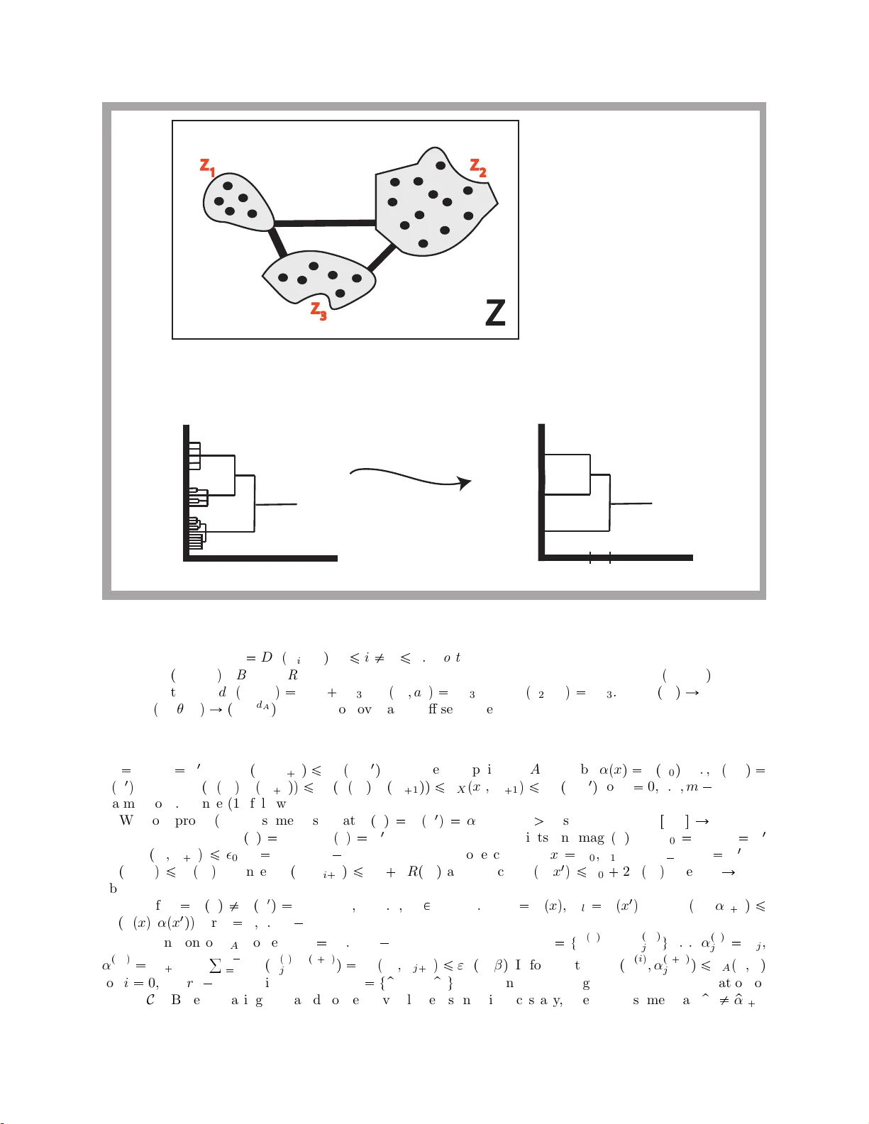
PERSISTENT CLUSTERING AND A THEOR E M OF J. KLEINBERG GUNNAR CARLSSON AND F ACUNDO M ´ EMOLI Abstract. W e construct a framework for st udying clustering algorithms, w hi c h includes t w o key ide as: p ersistenc e and functoriality . The first enco des the idea that the output of a clustering scheme should carry a multiresolution structure, the second the idea that one should b e able to compare the r esults of clustering algorithms as one v aries the data s et, for example by adding p oints or by applying functions to it. W e show that within this fr amew or k, one can prov e a theorem analogou s to one of J. Kleinberg [Kl e02], in whic h one obtains an existence and uniqueness theorem instead of a non-existence result. W e explore further prop erties of this unique sc heme, s tabilit y and con vergence are established. 1. Introduction Clustering techn iques play a very cen tral role in v arious parts of data analysis. They can give imp ortant clues to the structure of data sets, a nd therefore s uggest results and hypotheses in the underlying science. There are many interesting metho ds of clustering a v a ilable, whic h have b een applied to g o o d effect in dealing with man y datasets of in terest, and they are regar ded as imp ortant methods in explora tory data analysis . Despite b eing one of the most commonly used to ols for unsuper vised explor atory data ana lisys and despite its and extensive litera ture very little is known ab out the theo retical foundations o f clustering metho ds. The general ques tion of which metho ds are “ bes t”, or most appropriate fo r a particula r pro blem, or how sig nifica nt a particular clustering is has not b een addressed as frequently . One problem is tha t many metho ds inv o lve particular choices to b e made a t the o utset, for example how many clusters ther e should be, or the v alue o f a par ticular thresholding quantit y . In addition, some metho ds depe nd on artifacts in the data, such as the particular or der in which the ele ments are listed. In [Kle0 2], J. Kleinberg proves a very int eresting imp o ssibility result for the problem o f even defining a cluster ing scheme with so me r ather mild inv arianc e pr op erties. He also p oints out that his r esults shed lig h t o n the trade- offs one has to make in choosing cluster ing alg orithms. In this pap e r , we pro duce a v a riation on this theme, which we b elieve also has implica tio ns for how one thinks a bo ut a nd applies cluster ing alg orithms. In addition, w e study the pre c ise q ua nt itative (or metric) stability and c onv erge nc e /consitency of o ne particular clus tering scheme which is characterized by one o f o ur res ults. W e summarize the tw o main p oints in o ur appr oach. P ersis tence: W e b elieve that the o utput of clustering alg orithms shouldn’t b e a sing le set of clusters , but rather a more str uctured ob ject whic h enco des “ m ultiscale” or “multiresolution” information a bo ut the underlying data set. The r e a son is that data can often intrinsically p ossess str ucture at v ar io us differ e n t scales, as in Figure 1 b elow. Cluster ing techniques s hould reflect this structure, a nd provide metho ds for representing and analyzing it. Ideally , users should be prese n ted with a r eadily computable a nd pres ent able ob ject which will give him/her the option of choosing the pr op er scale for the analysis, or per haps int erpreting the m ultisc a le inv ar iant directly , rather than b e ing asked to choos e a scale or choo sing it for him/her. It is widely a ccepted that clustering is ultimately its e lf a to ol for explorato ry data ana lysis, [vLBD05]. In some sense, it is therefore totally acce pta ble to provide this multiscale inv a riant, whenever av ailable and let the user pick different scale thresholds that will yield different partitions of the data . Once we ac cept this, we can concentrate on answering theor etical questions r egarding schemes that output this kind of infor mation. Our analysis will Date : August 15, 2008. 2000 Mathematics Subje ct Classific ati on. Primary 62H30; Secondary 91C20. Key wor ds and phr ases. C l ustering, hierar c hical clustering, p ersistent topology , categories, functorialit y ,Gromov-Hausdorff distance. This w ork is supported by DARP A gran t HR0011-05-1-0007. 1 Figure 1. Dataset with multiscale structure and its co rresp onding dendr ogram. not, how ever, r ule out clustering metho ds that provide a one-sca le view of the da ta, since, formally , o ne ca n consider a s uch a scheme as o ne that at all scales gives the sa me informa tio n, cf. Example 2 .2 W e choose a particular wa y of representing this multiscale information, we use the formalism of p ersistent sets , which is in tro duced in Section 2, Definition 2.1. The idea o f showing the multiscale clustering view of the da taset is widely used in Gene ex pression data analy sis and it takes the form o f dendr o gr ams . F unctorialit y: As our repla cement for the constra ints discussed in [Kle02], w e will use instead the notion of functoriality which has b een a very useful framework for the dis c ussion o f a v ariety of problems within mathematics over the last few deca de s . F or a dis cussion o f ca tegories and functors, see [ML98]. Our idea is that clusters s ho uld b e viewed a s the sto chastic a nalogue of the ma thematical concept o f p ath c omp onents . Recall (see, e.g. [Mun75]) that the path comp onents of a topo logical spa ce X are the equiv alence clas ses of po int s in the s pa ce under the equiv alence r elation  path , w he r e, for x, y P X , we hav e x  path y if and only if ther e is a contin uous map ϕ : r 0 , 1 s Ñ X so that ϕ p 0 q  x a nd ϕ p 1 q  y . In o ther words, tw o p oints in X are in the sa me path co mpo nent if they ar e connected by a c ontin uous pa th in X . This set of comp onents is denoted by π 0 p X q . The assignment X Ñ π 0 p X q is said to b e functorial, in that g iven a contin uous map f : X Ñ Y ( morphism of top olo gical spaces ), ther e is a natural map of sets π 0 p f q : π 0 p X q Ñ π 0 p Y q , which is defined by requiring that π 0 p f q carries the path comp onent of a p oint x P X to the path co mpo ne nt of f p x q P Y . This notion has been critical in ma ny asp ects of g e ometry; it provides the basis for the metho ds of or ganizing geometric o b jects combinatorially which is referre d to as combinatorial or simplicial top ology . The input to clustering a lgorithms is not, of co urse, a top olog ical s pace. Rather, it is t y pically p oint cloud data , finite sets of p oints lying in a E uclidean space o f so me dimensio n, or p erhaps in s ome other metric space, s uch as a tree or a collection of w ords in so me alphab et equipp ed with a metric. W e will there fore think of it a s a finite metr ic space (see [Mun75] for a discuss ion o f metric spaces ). There is a na tural notion of what is meant by a map o f metr ic spaces, which one can think of as lo osely analog o us to contin uity . This notion has b een used in other contexts in the pas t, s ee for example [Is b64]. Similarly , we define a natural notion of what is meant by a morphism of the per sistent sets defined ab ov e, and require functoriality for the clustering alg o rithms we co nsider in ter ms o f these no tions of morphisms. F o r the time b e ing the rea der not familiar with the concept, can think o f functoriality as a no tio n of coa rse stability/consistency . By v arying the richness of the class of morphisms b etw een metric spac e s one can co ntrol how string ent are the conditions imp osed on the cluster ing algor ithms. F unctoriality can therefore b e interpreted as a notion o f c o arse st ability of these clustering algo rithms. In [McC0 2], the idea of using ca teg orical and functorial ideas in sta tis tics ha s b een propo sed as a formalism for defining what is meant b y statistical mo dels. One asp ect of o ur w or k is to show that the same ideas , which are so p ow erful in many o ther asp ects o f mathematics, can b e used to understand the na ture of algor ithms for a ccomplishing s tatistical tas ks. W e summarize the main features of our p oint o f view. (a) It makes explicit the notion of mu ltiscale r epresentation of the set of c lusters. (b) By v arying the degr e e of functorialit y (i.e. by considering differen t notions of morphis m on the domain of p oint clo ud data) one can reason ab out the existence and prop erties of v arious schemes. W e illustrate this 2 po ssibility in Section 4. In par ticular, ar e able to prove a uniqueness theorem for clustering algor ithms with one natur al notio n of functoriality . (c) Beyond the conceptual adv antages cited ab ov e, functoriality can b e directly useful in analyzing datasets. The prop erty can b e used to study qualitative geometric prop erties of point c loud data, in- cluding more subtle geometric information than clustering, such as pres e nc e of “lo opy” b ehavior or higher dimensional analog ues. See e.g . [CIdSZ08] for an example of this p oint o f view. W e will also pr esent a n example in Subsectio n 3 .2. In addition, the functoriality pro per t y can be us ed to analy ze functions on the datasets, by studying the be havior of sublevel sets of the function under clustering. O ne version of this idea builds pro babilistic versions of the Re eb gr aph . See [SMC07] for a num b er o f examples of how this ca n work. Other, different, no tions of stability of clustering schemes hav e app eared in the literatur e, see [Ra g 82, BDvLP06] a nd r eferences therein. W e touch upo n simila r co ncepts in Section 5. The o rganiza tio n of the pap er is as follows. In Section 2 we intro duce the main ob jects that mo del the output o f clustering alg orithms together with some imp ortant ex a mples. Section 3 int ro duces the concepts of catego ries and functors, a nd the idea o f functoriality is dis cussed. W e pres ent our main characteriz a tion results in Sectio n 4. The quantitativ e study of stabilit y and consistency is presented in Section 5. F urther applications of the concept of functor iality a re discussed in Section 6 and concluding remarks ar e presented in Sec tion 7. 2. Persistence In this s ection we define the ob jects whic h are the output of the cluster ing alg orithms we will b e work- ing with. These ob jects will enco de the notio n of “multiscale” o r “multiresolution” sets discussed in the int ro duction. Let P p X q denote the set of par titions of the (finite) set X . Definition 2.1 . A p ersistent s et is a p air p X , θ q , wher e X is a finite s et , and θ is a function fr om the non-ne gative re al line r 0 , 8q to P p X q so that the fol lowing pr op erties hold. (1) If r ¤ s , then θ p r q r efines θ p s q . (2) F or any r , ther e is a numb er ǫ ¡ 0 so that θ p r 1 q  θ p r q for al l r 1 P r r , r  ǫ s . If in additio n ther e exist s t ¡ 0 s.t. θ p t q c onsists of the single blo ck p artition for al l r ¥ t , then we say that p X , θ q is a dendrogra m . 1 The in tuition is that the set of blo cks o f the par tition θ p r q should b e reg arded as X viewed at sca le r . Example 2.1 . Let p X , d q be a finite metric space. Then we ca n asso cia te to p X , d q the p ersistent set whose underlying set is X , and wher e blo cks o f the par tition θ p r q consist o f the equiv alence classes under the equiv alence relation  r , where x  r x 1 if and only if there is a s equence x 0 , x 1 , . . . , x t P X so that x 0  x, x t  x 1 , a nd d p x i , x i  1 q ¤ r for all i . Example 2.2 . A more trivial example is one in which θ p r q is cons tant , i.e. c onsists of a s ing le pa rtition. This is the sca le free notion o f clus tering. Exa mples ar e k -means clustering and s pectr al cluster ing. Example 2.3. Here we co nsider the family of Agglomera tive Hiera rchical clustering techniques, [JD88]. W e (re)define these by the recursive pro ce dure describ ed next. Let X  t x 1 , . . . , x n u and let L denote a family of linkage functions , i.e. functions which one us es for defining the distance b etw ee n tw o clusters. Fix l P L . F or ea ch R ¡ 0 consider the equiv alence rela tion  l,R on blo cks of a partition Π P P p X q , given by B  l,R B 1 if and only if ther e is a sequence of blo cks B  B 1 , . . . , B s  B 1 in Π with l p B k , B k  1 q ¤ R for k  1 , . . . , s  1. Consider the sequenc e s r 1 , r 2 , . . . P r 0 , 8q and Θ 1 , Θ 2 , . . . P P p X q given by Θ 1 :  t x 1 , . . . , x n u and fo r i ¥ 1, Θ i  1  Θ i {  l,r i where r i :  min t l p B , B 1 q , B , B 1 P Θ i , B  B 1 u . Finally , we define θ l : r 0 , 8q Ñ P p X q by r ÞÑ θ l p r q :  Θ i p r q where i p r q :  max t i | r i ¤ r u . Standard c hoices for l are single linkage : l p B , B 1 q  min x P B min x 1 P B 1 d p x, x 1 q ; c omplete linkage l p B , B 1 q  max x P B max x 1 P B 1 d p x, x 1 q ; a nd aver age linkage : l p B , B 1 q  ° x P B ° x 1 P B 1 d p x,x 1 q # B  # B 1 . It is e asily verified that the notio n discussed in E x ample 2.1 is e quivalent to θ l when l is the sing le link age function. Note that, unlike the us ua l definition of agglo merative 1 In the paper we will be using the word dendrogram to r efer both to the ob ject defined here and to the s tandard graphical represen tation of them. 3 hierarchical cluster ing, a t each step of the inductiv e definition we a llow for more than tw o cluster s to b e merged. W e will b e using the per sistent se ts which arise out of Example 2.1. It is of course the case that the per sistent s et carries muc h mor e information than a single set o f clusters. One ca n ask whether it carrie s to o m uch informatio n, in the sense that either (a) one cannot obtain useful in terpretations from it or (b) it is computationally intractable. W e cla im that it ca n usually b e usefully interpeted, a nd can b e effectively and efficiently computed. One ca n obser ve this as follows. Since there are o nly a finite n umber of partitions of X , a p ers is ten t set Q gives a partition of R  int o a finite co llection I of in terv als of the form r r , r 1 q , together with one in ter v al o f the form r r , 8q . F or ea ch s uch interv al, every num b er in the interv a l c o rresp onds to the s ame par tition of X . W e claim that knowledge of these interv als is a key piece o f information ab out the p ersis ten t sets arising from Exa mples 2 .1 and 2.3 ab ov e. The reason is that lo ng interv a ls in I corresp ond to la rge rang es o f v alues of the sca le parameter in which the asso cia ted cluster decomp os itio n do esn’t change. One would then regar d the partitio n into cluster s cor resp onding to tha t interv al as likely to r epresent s ignificant structure present a t the g iven ra nge of scales . If there is only one long interv al (aside from the infinite in terv al of the form r r , 8q ) in I , then one is led to b elieve that there is o nly one interesting r ange o f scales, with a unique decomp osition in to clusters. How ever, if there are more tha t o ne lo ng interv al, then it sug g ests that the ob ject has significant multiscale be havior, see Fig ure 1. Of c o urse, the deter mina tion of what is “long” and what is “shor t” will be problem dep endent, but c ho o sing thre s holds for the length of the interv a ls will give definite ra nges of scales. As for the computability , the p ersistent sets asso ciated to a finite metric space can b e readily computed using (convenien tly mo dified) hier archical clustering techniques, or the metho ds of per sistent ho mology (see [ZC0 4]). 3. Ca tegories, functors and functorial ity 3.1. Definitio ns and E xamples. In this section, w e will give a brief description of the theor y of categor ies and functor s, which will b e the fr amework in which we state the cons tr aints we will requir e of o ur clus ter ing algorithms. An ex cellent refer ence for these ideas is [ML 9 8]. Categorie s ar e useful mathematical co nstructs that enco de the nature o f cer tain ob jects of interest together with a set of admissible/interesting/useful maps betw een them. This forma lism is extremely us eful for studying cla s ses of mathematical ob jects which shar e a common structure, such as sets , groups, vector spaces, or top olog ical spaces. The de finitio n is as follows. Definition 3. 1. A c ate gory C c onsists of  A c ol le ction of obje cts ob p C q (e.g. sets, gr ou ps, ve ctor sp ac es, etc.)  F or e ach p air of obje cts X , Y P ob p C q , a set M or C p X , Y q , the morphisms fr om X to Y (e.g. map s of sets fr om X t o Y , homomorphisms of gr oups fr om X to Y , line ar tr ansformations fr om X to Y , etc. r esp e ctively)  Comp osition op er ations:  : M or C p X , Y q  M or C p Y , Z q Ñ M or C p X , Z q , c orr esp onding to c omp osition of set maps, gr oup homomorph isms, line ar tr ansformations, etc.  F or e ach obje ct X P C , a distinguishe d element id X P M or C p X , X q The c omp osition is assume d to b e asso ciative in the obvious sen se, and for any f P M or C p X , Y q , it is assume d that id Y  f  f and f  id X  f . Here a r e the relev ant examples for this pap er. Example 3 .1. W e will constr uct three catego ries M iso , M mon , and M gen , whos e collections of ob jects will all consist of the c ollection of finite metric spa ces. Let p X , d X q and p Y , d Y q denote finite metr ic spaces. A set map f : X Ñ Y is sa id to be distanc e non incr e asing if for all x, x 1 P X , we hav e d Y p f p x q , f p x 1 qq ¤ d X p x, x 1 q . It is eas y to ch eck that co mpo s ition of distance non-incr easing maps are also distance non- increasing, and it is also clear that id X is a lwa ys distance non-incr easing. W e therefor e hav e the category M gen , whos e ob jects are finite metric spa c es, a nd s o that for any ob jects X and Y , M or M gen p X , Y q is the set of dista nce non-increas ing maps fro m X to Y , cf. [Isb64] for a nother use of this class o f maps. W e say that a dis ta nce non-increas ing map is monic if it is an inclusio n a s a set map. It is clear co mpos itions of monic maps are 4 monic, a nd that all identit y maps ar e monic, so we hav e the new catego ry M mon , in which M or M mon p X , Y q consists of the mo nic dis tance non-increa s ing maps. Finally , if p X , d X q and p Y , d Y q are finite metr ic s paces, f : X Ñ Y is an isometry if f is bijective and d Y p f p x q , f p x 1 qq  d X p x, x 1 q for all x and x 1 . It is clear that a s ab ov e, one ca n for m a categ ory M iso whose ob jects a re finite metric spaces and whose mor phis ms a re the isometries. It is clear that we hav e inclusions (3–1) M iso  M mon  M gen of sub categ ories (defined a s in [ML98]). Note that a ltho ugh the inclus io ns a re bijections on ob ject sets, they are prop er inclusions on mor phism sets, i.e. they a re not in general surjective. W e will also cons tr uct a categor y of p ersistent sets . Example 3.2. Let p X , θ q , p Y , η q be p ersistent sets. F o r any partition Π of a set Y , and any set map f : X Ñ Y , we define f  p Π q to b e the partition of X w ho se blocks are the s ets f  1 p B q , as B rang e s over the blo cks of Π. A ma p of sets f : X Ñ Y is said to b e p ersistenc e pr eserving if for each r P R , w e hav e that θ p r q is a refinement of f  p η p r qq . It is easily verified that the comp osite o f p ers is tence preserving maps is p ersistence preserving , and that any identit y map is per sistence pre serving, and it is therefo re clear that we may define a category P whose ob jects ar e per sistent se ts , and wher e M or P pp X , θ q , p Y , η qq consists of the set maps fro m X to Y which a re p ers istence pres erving. A simple example is shown in Figure 2. A ’ B’ C ’ 1 1 1 2 A B C 2 2 2 {{A},{B},{ C }} {{A ’ ,B’},{C’}} f(A ) = A ’ f(B) = B’ f(C) = C ’ Figure 2. Two p ersis ten t sets p X , θ q and p Y , η q represented b y their dendrog rams. On the left one defined in the set X  t A, B , C u and on the right one defined o n the set Y  t A 1 , B 1 , C 1 u . Consider the given set map f : X Ñ Y . Then we see that f is p ers istence preserving since for ea ch r ¥ 0, the par tition θ p r q is a refinement of f  p η p r qq . Indeed, there are three in ter esting ranges of v alues of r . Pick for ex ample r like in the orange shaded area: r P r 1 , 2 q . Then η p r q  tt A 1 , B 1 u , t C 1 uu and hence f  p η p r qq  t f  1 pt A 1 , B 1 uq , t f  1 p C 1 quu  tt A, B u , t C uu which is indeed re fined by θ p r q  tt A u , t B u , t C uu . One pro ceeds similary for the o ther tw o cases . W e next int ro duce the key co ncept in our discussion, that o f a functor . W e give the formal definition first. Definition 3. 2. L et C and D b e c ate gories. Then a functor fr om C to D c onsists of  A map of sets F : ob p C q Ñ ob p D q  F or every p air of obje cts X , Y P C a map of sets Φ p X , Y q : M or C p X , Y q Ñ M or D p F X, F Y q so that (1) Φ p X , X qp id X q  id F p X q for al l X P ob p C q (2) Φ p X , Z qp g  f q  Φ p Y , Z qp g q  Φ p X , Y qp f q for al l f P M or C p X , Y q and g P M or C p Y , Z q Remark 3.1. In the inter est of clarity, we often r efer to t he p air p F, Φ q as a single let t er F . Se e diagr am (3–2) in Example 3.5 b elow for an example. A mor phism f : X Ñ Y which has a tw o sided inv ers e g : Y Ñ X , so that f  g  id Y and g  f  id X , is called an isomorphism . Two o b jects which are isomor phic ar e intuitiv ely thought of as “s tructurally 5 indistinguishable” in the sense that they are iden tica l except for naming or choice of co o rdinates. F or example, in the category of sets, the sets t 1 , 2 , 3 u and t A, B , C u are iso morphic, since they ar e identical except for choice made in lab elling the elements. W e illus trate this definition with some examples. Example 3. 3. (F orgetful functors) When o ne has t wo categ ories C and D , where the ob jects in C ar e ob jects in D eq uipped with some additional structure a nd the mo rphisms in C are simply the mor phisms in D which prese r ve that structure, then we obtain the “ forgetful functor ” from C to D , which carr ies the ob ject in C to the same o b ject in C , but regarde d witho ut the additional str ucture. F or example, a g roup can b e r egarded as a set with the a dditional structure of multiplication and inv er se maps, and the group homomorphisms are simply the set maps which r e s pec t that structure. Accordingly , we hav e the functor from the category of gr oups to the ca tegory of se ts which “ forgets the multiplication and inv erse” . Similar ly , we have the forgetful functor fr om P to the ca tegory of s e ts, which forgets the pr esence of θ in the per sistent set p X , θ q . Example 3.4. The inclusio ns M iso  M mon  M gen are bo th functor s. An y g iven clustering scheme is a pro cedure F which takes as input a finite metric spac e p X , d X q , that is, an ob ject in ob p M gen q , and de livers as o utput a p ersis tent se t, that is, an o b ject in ob p P q . The concept of functoria lit y refers to the additio na l condition that the clustering pr o cedure maps a pair o f input ob jects int o a pair of output ob jects in a manner which is consis tent/stable with resp ect to the morphisms attached to the input a nd output spaces. When this ha ppens , we say that the clustering scheme is functorial . This notion o f co nsistency/stability is made prec is e in Definition 3.2 a nd des c rib ed by diagr am (3–2). Now, the idea is to regard clustering algorithms (that output a p ersistent set) as functor s. Assume for instance w e w a n t to consider “stability” to all dista nce non-incr e asing ma ps. Then the cor rect categ ory of inputs (finite metric s pa ces) is M gen and the categor y of o utputs is P . Accor ding to Definition 3.2 in or der to view a clustering scheme a s a functor we need to sp ecify (1) how it maps ob jects of M gen (finite metric spaces) into ob jects o f P (per sistent sets), and (2) how a v alid morphism/map f : p X , d X q Ñ p Y , d Y q betw een t wo ob jects p X , d X q and p Y , d Y q in the input spac e /categor y M gen induce a map in the output categor y P , see diag ram (3–2) b elow. W e exemplify this throug h the constructio n of the key exa mple fo r this pap er. Example 3.5. W e define a functor R gen : M gen Ñ P as follows. F or a finite metric space p X , d X q , we define R gen p X , d X q to b e the per sistent set p X , θ d X q , where θ d X p r q is the partition a sso ciated to the equiv alence r elation  r defined in Example 2.1. This is clear ly an ob ject in P . W e also define how R gen acts on ma ps f : p X , d X q Ñ p Y , d Y q : The v alue of R gen p f q is simply the se t map f reg arded as a morphism fr o m p X , θ d X q to p Y , θ d Y q in P . That it is a morphism in P is easy to chec k . This functorial construction is r epresented through the dia gram b elow: (3–2) p X , d X q R gen / / f   p X , θ d X q R gen p f q   p Y , d Y q R gen / / p Y , θ d Y q where R gen p f q is pe rsistence preserving . Example 3.6. By r estricting R gen to the s ubca tegories M iso and M mon , we obtain functors R iso : M iso Ñ P and R mon : M mon Ñ P . Example 3 .7. Let λ b e any pos itiv e real num b er. Then we define a functor σ λ : M gen Ñ M mon on ob jects by σ λ p X , d X q  p X , λd X q and on mor phisms by σ λ p f q  f . O ne easily verifies that if f s atisfies the conditions for b eing a morphism in M gen from p X , d X q to p Y , d Y q , then it readily satisfies the conditions to b e a morphism from p X , λd X q to p Y , λd Y q . Similar ly , we define a functor s λ : P Ñ P by setting s λ p X , θ q  p X , θ λ q , w he r e θ λ p r q  θ p r λ q . In Section 4 we will b e showing our main results. W e will now hav e a brief disgr ession to discuss other situations in which, in our opinion, the concept of functoria lit y can b e useful. 6 3.2. In trinsic V alue of F unc to rialit y. By studying functorial metho ds of c lus tering, it is p ossible to recov e r qualitative asp ects of the geometric structure of a datas et. W e illus tr ate this idea with a “toy” example. W e supp os e that we hav e a p oint cloud data which is co ncentrated around the unit circle. W e consider the pro jection of the data o n to the x -axis, and cov er the axis with tw o (ov erla pping) interv a ls U a nd V , pictured on the left in Figure 3 b elow as b eing red and yello w, with or ange intersection. By considering tho s e po rtions of the dataset whose x -co ordinate lie in U and V resp ectively , we obta in the red and yello w subsets o f the dataset pictur e d o n the r ig ht b elow. Their in ter section is pic tur ed a s or ange, and the a rrows indicate that we hav e inclusions of the intersection into each of the pieces. Nex t, we note that if Figure 3. L eft : Covering of a cir cle b y t wo interv als . Center : Corresp onding diag ram of comp onents. Right : Homotopy colimit of dia g ram in center figure. we are dealing with a functorial c lus tering scheme, a nd c luster each o f these subsets, we obtain the diag ram of clusters in the center of Figure 3. This is now a very s imple co m binatorial ob ject. There is a top olog ical co nstruction known as the homotopy c olimit , which given any dia g ram of sets of any shap e reconstr ucts a s implicial set (a s lightly more flexible version of the notion of simplicial complex), and in particula r a space . T o first approximation, one builds a vertex for e very element in any set in the diagram, a nd an edge betw e en any tw o element s which are connected by a map in the diagra m, and then attaches higher o rder simplices according to a well defined pro cedure. In the case o f the diagr am ab ov e, this constructs the s pace g iven in the rightmost part o f Fig ur e 3 . The details of the theo r y of simplicial sets and homotopy colimits are be yond the sco pe o f this pap er. A thorough exp os ition is given in [BK7 2]. F unctoriality is also quite useful when one is interested in studying the qualita tiv e b ehavior of a r eal-v alued function f on a datas et, for example the output of a dens ity estimator. Then it is useful to study the set of clusters in sublevel and sup erlevel se ts of f , and under standing how the cluster s b ehav e under changes in the thresholds can help one understand the pre s ence of sa ddle p oints and higher index cr itical p oints of the function. One e x ample of this is t wo-para meter p ersistence constructio ns, [CSZon]. In this case, there is more structure than just p ers is ten t sets (trees/ dendrogra ms) as defined in this pa p er . W e will elab or ate on another applicatio n of functor iality in Sectio n 6. 4. Resul ts W e now study different clustering a lg orithms us ing the idea of functor iality . W e hav e 3 p o s sible “input” categorie s order ed by inclusion (3– 1). The idea is that studying functoriality over a la r ger c a tegory will be more str ingent/demanding than r equiring functor iality ov er a smalle r one. W e now co ns ider different clustering alg o rithms and study whether they a re functorial over our c ho ic e of the input category . W e start by analyzing functoriality over the least demanding one, M iso , then we pr ov e a uniqueness res ult for functoriality ov er M gen and fina lly we study how r elaxing the conditions imp o sed by the morphisms in M gen , namely , by restricting o urselves to the sma ller but intermediate catego ry M mon , we p ermit more functorial c lus tering a lgorithms. 4.1. F unctoralit y o v e r M iso . This is the sma llest category we will deal with. The morphisms in M iso are simply the bijective maps b etw een da ta sets which preser ve the distance function. As s uch, functoriality of a cluster ing algorithms over M iso simply means that the o utput of the scheme do esn’t depend on any artifacts in the dataset, such as the way the p oints are named or the way in whic h they ar e ordered. Her e are some ex amples which illustrate the idea.  The k -me ans algorithm (see [JD88]) is in pr inc iple allow ed by our framework since ob p P q contains all constant pe r sistent sets. How ever it is not functor ia l on any of o ur input catego ries. It dep ends bo th on a paramter k (num b er of clusters ) and on an initial choices of mea ns, and is not ther efore depe ndent o n the metric structure alone. 7  A gglomer ative hier ar chic al clustering , in s tandard form, as describ ed for example in [JD88], be g ins with p oint cloud data a nd co nstructs a binary tree (or dendrogra m) which describ es the mer ging of clusters as a threshold is increas ed. The lack of functoriality co mes from the fac t that when a single thr e shold v alue corr esp onds to mo re than one data p oint, one is forced to choo se an order ing in order to decide which p oints to “agglomer ate” first. This can e asily b e modified by r elaxing the requirement that the tr ee be bina ry . This is what we did in Example 2.3 In this case, one can view these metho ds as functorial on M iso , where the functor takes its v alues in ar bitr ary r o oted trees. It is understo o d that in this case , the notion o f mo r phism for the output ( P ) is simply isomor phism of ro oted trees. In contrast, we see next that amo ngst these metho ds, when we impo se that they b e functorial over the larger (mor e demanding ) categ o ry M gen then only one o f them passes the test. 2  Sp e ctr al clu stering . As describ ed in [vL07], typically , spectr al methods co nsist of t wo differen t lay ers. They firs t define a la placian matrix o ut of the dissimilarity matrix (given by d X in our case) and then find eig env alues and eigenvectors of this op erator. The s e cond lay er is as follows: a natura l nu mber k m ust b e sp ecified, a pr o jection to R k is p erformed using the eigenfunctions, and clusters are fo und by an application o f the k -means clustering algorithm. Clea rly , op erations in the second lay er will fail to be functorial as they do not dep end o n the metr ic alone. Ho wev er, the pr o cedure underlying in the first lay er is clea rly functorial on M iso as eigenv alue computations are changed by a p ermutation in a well defined, natural, wa y . 4.2. F unctoralit y ov er M gen : a uni queness theo rem. In this section, a s an ex ample a pplica tion of the conceptual fr amework of functoriality , we will prove a theor em of the s ame flavor as the main theorem of [Kle02], exc ept that we prove existence and uniqueness on M gen instead o f imp ossibility in our context. Before stating and proving our theo r em, it is interesting to p oint out why complete link age and av erag e link age (agglomera tive) clus tering, a s defined in Exa mple 2.3 are not functorial on M gen . A simple example explains this: co nsider the metric spaces X  t A, B , C u with metric given by the edge lengths t 4 , 3 , 5 u and Y  p A 1 , B 1 , C 1 q with metric g iven by the edge lengths t 4 , 3 , 2 u , a s given in Fig ure 4. Obviously the map f from X to Y with f p A q  A 1 , f p B q  B 1 and f p C q  C 1 is a morphism in M gen . Note that for example for r  3 . 5 (shaded regions o f the dendro grams in Figure 4) w e hav e that the partition of X is Π X  tt A, C u , B u whereas the partition of Y is Π Y  tt A 1 , B 1 u , C 1 u and th us f  p Π Y q  tt A, B u , t C uu . Therefore Π X do es not refine f  p Π Y q as r equired by functoria lity . The s a me constr uction yields a counter-example for av er age link age. Theorem 4.1. L et Ψ : M gen Ñ P b e a functor which sat isfies the fol lowing c onditions. (I): L et α : M gen Ñ S ets and β : P Ñ S ets b e the for getful fu n ctors p X , d X q Ñ X and p X , θ q Ñ X , which for get the metric and p artition re sp e ctively, and only “r ememb er” t he u nderlying sets X . Then we assu m e that β  Ψ  α . This me ans that the underlying set of the p ersistent set asso ciate d to a metric sp ac e is just t he underlying set of the m et ric sp ac e. (I I): F or δ ¥ 0 let Z p δ q  pt p, q u ,  0 δ δ 0  q denote the two p oint metric sp ac e with underlying set t p, q u , and wher e dist p p, q q  δ . Then Ψ p Z p δ qq is the p ersistent set pt p, q u , θ Z p δ q q whose underlying set is t p, q u and wher e θ Z p δ q p t q is the p artition with one element blo cks when t  δ and it is the p artition with a single two p oint blo ck when t ¥ δ . (I I I): Given a fin ite metric sp ac e p X , d X q , let sep p X q :  min x  x 1 d X p x, x 1 q . Write Ψ p X , d X q  p X , θ Ψ q , then for any t  sep p X q , the p artition θ Ψ p t q is the discr ete p artition with one element blo cks. Then Ψ is e qual to the functor R gen . Pr o of. Let Ψ p X , d X q  p X , θ Ψ q . F or e a ch r ¥ 0 we will prove that (a) θ d X p r q is a refinement of θ Ψ p r q and (b) θ Ψ p r q is a r efinemen t of θ d X p r q . 2 The result in Theorem 4.1 is actually more p ow erf ul in that it states that there is a unique functor f rom M gen to P that satisfies certain natural conditions. 8 B 5 3 4 A C X 2 3 4 C A B 1 5 0 X 2 3 4 C’ A ’ B’ 1 5 0 Y B’ 4 C’ 3 2 Y A’ Figure 4. An example that s hows why complete link ag e fails to b e functoria l o n M gen . Then it will follow that θ d X p r q  θ Ψ p r q for all r ¥ 0, which shows that the ob jects ar e the same. Since this is a situation where, g iven any pair of ob jects, ther e is a t mo s t one morphism betw een them, this a lso determines the effect of the functor on morphisms. Fix r ¥ 0. In or der to obtain (a) we need to pr ov e that whenever x, x 1 P X lie in the same blo ck o f the partition θ d X p r q , that is x  r x 1 , then they b oth lie in the s ame blo ck of θ Ψ p r q . It is enough to pr ov e the following Clai m : whenever d X p x, x 1 q ¤ r then x and x 1 lie in the same blo ck of θ Ψ p r q . Indeed, if the claim is true, and x  r x 1 then one can find x 0 , x 1 , . . . , x n with x 0  x , x n  x 1 and d X p x i , x i  1 q ¤ r for i  0 , 1 , 2 , . . . , n  1. Then, inv o king the claim for all pairs p x i , x i  1 q , i  0 , . . . , n  1 one would find that: x  x 0 and x 1 lie in the same blo ck of θ Ψ p r q , x 1 and x 2 lie in the same blo ck of θ Ψ p r q , . . . , x n  1 and x n  x 1 lie in the sa me blo ck of θ Ψ p r q . Hence, x and x 1 lie in the sa me blo ck of θ Ψ p r q . So, let’s prove the cla im. Assume d X p x, x 1 q ¤ r , then the function g iven by p Ñ x, q Ñ x 1 is a morphism g : Z p r q Ñ p X , d X q in M gen . This means that we obta in a morphis m Ψ p g q : Ψ p Z p r qq Ñ Ψ p X , d X q in P . But, p and q lie in the s ame blo ck of the partition θ Z p r q by definition of Z p r q , and functoriality ther efore guarantees that Ψ p g q is per sistence pr eserving (recall Example 3.2) a nd hence the elements g p p q  x a nd g p q q  x 1 lie in the sa me blo ck of θ d X p r q . This concludes the pr o of of (a). F or condition (b), as sume that x and x 1 belo ng to the same blo ck o f the partition θ Ψ p r q . W e will prove that ne c e ssarily x  r x 1 . This of course will imply tha t x and x 1 belo ng to the sa me blo ck of θ d X p r q . Consider the metric space p X r r s , d r r s q whose p oints a re the equiv alence classes of X under the equiv alence relation  r , and where the metr ic d r r s : X r r s  X r r s Ñ R  is defined to b e the max imal metric p oint wisely less than or equa l to W , where for tw o p oints B and B 1 in X r r s (equiv alence clas ses of X under  r ), W p B , B 1 q  min x P B min x 1 P B 1 d X p x, x 1 q . 3 It follows from the definition of  r that if tw o e q uiv alence clas ses are distinct, then the distance b etw een them is ¡ r . This means that sep p X r r sq ¡ r . 3 See Section 5 for a similar, explicit construction. 9 W rite Ψ p X r r s , d r r s q  p X r r s , θ r r s q . Since sep p X r r sq ¡ r , h yp othes is (II I) now directly shows that the blo cks of the partitio n θ r r s p r q are exactly the e q uiv alence classes of X under the equiv alence rela tion  r , that is θ r r s p r q  θ d X p r q . Finally , consider the morphism π r : p X , d X q Ñ p X r r s , d r r s q in M gen given on elements x P X by π r p x q  r x s r , where r x s r denotes the equiv alence class of x under  r . By functoriality , Ψ p π r q : p X , θ Ψ q Ñ p X r r s , θ r r s q is p ers istence preserving, and therefore, θ Ψ p r q is a r efinement of θ r r s p r q  θ d X p r q . This is depicted as follows: p X , d X q Ψ / / π r   p X , θ d X q Ψ p π r q   p X r r s , d r r s q Ψ / / p X r r s , θ r r s q This concludes the pro of of (b).  W e sho uld p oint out that a nother characterization of single link age has b een obta ine d in the bo o k [JS7 1]. 4.2.1. Comments on Kleinb er g’s c onditions. W e c onclude this section by obser ving that a nalogues of the three (ax io matic) pro p er ties consider ed by Kleinberg in [K le02] hold for R gen . Kleinberg’s first condition was sc ale-invarianc e , which as serted that if the dis tances in the underlying po int cloud data were multip lied by a cons ta n t p ositive multiple λ , then the resulting clus ter ing decomp osition should b e identical. In our cas e, this is r eplaced b y the co nditio n that R gen  σ λ p X , d X q  s λ  R gen p X , d X q , which is trivia lly sa tisfied. Kleinberg’s seco nd condition , richness , asserts that any par tition of a data set ca n be o btained as the result o f the g iven clustering scheme for s ome metric o n the da taset. In o ur context, partitions ar e replaced by p e rsistent sets. Ass ume that there exist t P R s.t. θ p t q is the single blo ck partition, i.e., impo se that the per sistent set is a dendro gram (cf. Definition 2.1). In this case, it is easy to chec k tha t any such p ersis ten t set can b e obtained as R gen ev aluated for some (pseudo)metr ic on some dataset. Indeed, 4 let p X , θ q P ob p P q . Let ǫ 1 , . . . , ǫ k be the (finitely many) tr ansition/disco ntin uit y p oints of θ . F or x, x 1 P X define d X p x, x 1 q  min t ǫ i u s.t. x, x 1 belo ng to sa me blo ck of θ p ǫ i q . This is a pseudo metric on X . Indeed, pick p oints x, x 1 and x 2 in X . Let ǫ 1 and ǫ 2 be minimal s.t. x, x 1 belo ng to the s a me blo ck of θ p ǫ 1 q and x 1 , x 2 belo ng to the s a me blo ck of θ p ǫ 2 q . Let ǫ 12 :  max p ǫ 1 , ǫ 2 q . Since p X , θ q is a p ersistent set (Definition 2.1), θ p ǫ 12 q m ust hav e a blo ck B s.t. x, x 1 and x 2 all lie in B . Hence d X p x, x 2 q ¤ ǫ 12 ¤ ǫ 1  ǫ 2  d X p x, x 1 q  d X p x 1 , x 2 q . Finally , Kleinberg’s third condition , c onsistency , could be viewed as a r udimentary ex a mple o f functori- ality . His mor phisms ar e similar to the ones in M gen . 4.3. F unctorialit y o ver M mon . In this sectio n, we illustra te how relaxing the functoriality p ermits more clustering alg orithms. In other words, we will restric t ours e lves to M mon which is smaller (less stringent) than M gen but lar g er (mor e str ingent) than M iso . W e co nsider the restriction of R gen to the catego ry M mon . F or any metric space and every v alue of the p ers is tence para meter r , we will obtain a partition of the under ly ing set X of the metric spa c e in ques tion, a nd the set of equiv a le nce classe s under  r . F or any x P X , let r x s r be the equiv alence cla ss o f x under the equiv alence relatio n  r , and define c p x q  # r x s r . F or any integer m , we now define X m  X by X m  t x P X | c p x q ¥ m u . W e note that for any morphism f : X Ñ Y in M mon , we find that f p X m q  Y m . This pro per ty clear ly do es not ho ld for more gener al morphisms. F or every r , we ca n now define a new eq uiv alence r e lation  m r on X , which re fines  r , by requiring tha t each equiv alence cla ss of  r which has ca rdinality ¥ m is an equiv alence class of  m r , and that for any x for which c p x q  m , x defines a singleton equiv alence class in  m r . W e now obtain a new per sistent set p X , θ m q , where θ m p r q will denote the partition asso ciated to the equiv alence relation  m r . It is readily c heck ed that X Ñ p X , θ m q is functorial on M mon . This scheme could b e motiv ated by the intuit ition that one does not reg ard clusters o f small cardinality as significant, a nd therefore mak es p oints lying in s mall clusters in to sing letons, wher e one can then remov e them a s repr esenting “o utliers”. 4 W e only prov e triangle inequality . 10 5. Metric st ability and convergence pr o per ties of R gen In this s ection w e briefly discuss some further prop erties of R gen (single link age dendrograms). W e will provide q ua nt itative results on the stability and c onver genc e/c onsitency prop erties of this functor (algo- rithm). T o the best o f our knowledge, the only other related results obtained for this alg orithm app ear in [Har81]. The iss ues of stability and conv e rgence/co nsistency of clus ter ing algo rithms hav e brought back into attent ion recently , see [vLBD05, BDvLP0 6] and references therein. In Theor em 5.1 besides proving sta bility , we prove convergence in a simple setting. Given finite metr ic spaces p X , d X q and p Y , d Y q , our goa l is to define a distance b etw ee n the p ersistence ob jects θ d X and θ d Y resp ectively pr o duced by R gen . W e know that this functor actually outputs dendr ograms (ro oted trees ), which hav e a na tural metric structure attached to them. Moro ever, it is well known that ro oted tr ees ar e uniquely characterized by their distance matrix, [SS0 3]. F or a finite metric space p X , d X q consider the derived metric spa ce p X , ε X q with the sa me underlying set and metric (5–3) ε X p x, x 1 q :  min t ε ¥ 0 | x  ε x 1 u . Note that p X , θ d X q can therefore obviously b e regar ded as the metric space p X , ε X q , cf. with the co n- struction o f the metric in section 4.2.1. W e now chec k that indeed ε X defines a metric on X . Prop ositio n 5. 1. F or any finite metric sp ac e p X , d X q , p X , ε X q is also a metric sp ac e. Pr o of. (a) Since d X is a metric o n X , it is obvious that ε X p x, x 1 q  0 implies x  x 1 . (b) Symmetry is also obvious since  ε is an equiv alence relatio n. (c) T riangle inequa lit y: Pick x, x 1 , x 2 P X . Let ε X p x, x 1 q  ε 1 and ε X p x 1 , x 2 q  ε 2 . Then, there exis t p oints a 0 , a 1 , . . . , a j and b 0 , b 1 , . . . , b k in X with a 0  x , a j  x 1  b 0 , b k  x 2 and d X p a i , a i  1 q ¤ ε 1 for i  0 , . . . , j  1 and d X p b i , b i  1 q ¤ ε 2 for i  0 , . . . , k  1. Co nsider the po int s t c i u j  k  1 i  0  t a 0 , . . . , a j , b 1 , . . . , b k u . Then d X p c i , c i  1 q ¤ max p ε 1 , ε 2 q ¤ ε 1  ε 2 . Hence x  ε 12 x 2 with ε 12  ε 1  ε 2 and then by definition (5–3), ε X p x, x 2 q ¤ ε X p x, x 1 q  ε X p x 1 , x 2 q .  In order to compare the outputs of R gen on tw o different finite metric spaces p X , d X q and p X 1 , d X 1 q we will instead compa re the metric space r epresentations of those outputs, p X , ε X q and p X 1 , ε X 1 q , resp ectively . F or this purp ose, we choo s e to work with the Gro mov-Hausdorff distance which we define now, [B B I01]. Definition 5. 1 (Co rresp ondence) . F or sets A and B , a subset R  A  B is a co rresp ondence (b et we en A and B ) if and and only if   a P A , ther e exists b P B s.t. p a, b q P R   b P B , ther e exists a P X s.t. p a, b q P R Let R p A, B q denote the set of all p ossible corres po ndences b et ween sets A a nd B . Consider finite metric spac es p X , d X q and p Y , d Y q . Let Γ X,Y : X  Y  X  Y Ñ R  be g iven by p x, y , x 1 , y 1 q ÞÑ | d X p x, x 1 q  d Y p y , y 1 q| . Then, the Grom o v-Hausdorff distance b etw een X and Y is given by (5–4) d G H p X , Y q :  inf R P R p X,Y q max p x,y q , p x 1 ,y 1 qP R Γ X,Y p x, y , x 1 , y 1 q Remark 5.1. This expr ession defines a metric on the set of (isometry classes of ) finite metric sp ac es, [BBI01] (The or em 7.3.30). One has : Prop ositio n 5. 2. F or any finite metric sp ac es p X , d X q and p Y , d Y q d G H pp X , d X q , p Y , d Y qq ¥ d G H pp X , ε X q , p Y , ε Y qq . Pr o of. Let η  d G H pp X , d X q , p Y , d Y qq and R P R p X , Y q s.t. | d X p x, x 1 q  d Y p y , y 1 q| ¤ η for all p x, y q , p x 1 , y 1 q P R . Fix p x, y q and p x 1 , y 1 q P R . Let x 0 , . . . , x m P X b e s.t. x 0  x , x m  x 1 and d X p x i , x i  1 q ¤ ε p x, x 1 q for all i  0 , . . . , m  1. Let y  y 0 , y 1 , . . . , y m  1 , y m  y 1 P Y be s.t. p x i , y i q P R for a ll i  0 , . . . , m (this is po ssible b y definition of R ). Then, d Y p y i , y i  1 q ¤ d X p x i , x i  1 q  η ¤ ε X p x, x 1 q  η for a ll i  0 , . . . , m  1 11 and hence ε Y p y , y 1 q ¤ ε X p x, x 1 q  η . By exchanging the role s of X and Y one obtains the inequality ε X p x, x 1 q ¤ ε Y p y , y 1 q  η . This means | ε X p x, x 1 q  ε Y p y , y 1 q| ¤ η . Since p x, y q , p x 1 , y 1 q P R are arbitr a ry , and upo n r ecalling the definition of the Gromov-Hausdorff distance we o btain the desired co nclusion.  Prop ositio n 5 .2 will allow us to qua n tify stability and c onver genc e . W e provide deter ministic arguments. The same constr uc tio n, essentially , y ields similar results under the assumption that p Z, d Z q is enriched with a (Borel) probability measur e a nd one takes i.i.d. samples w.r.t. this pro bability measure. Assume p Z, d Z q is an underlying (p erhaps “contin uous” ) metric s pace from which differen t finite sa mples are drawn. W e w ould like to s ee, quantitativ ely , (1 ) how the results yielded b y R gen differ when applied to those different sample sets (which p ossibly contain different num b ers of p oints), this is stability and (2) that when the underlying metric space is par titioned, there is c onver genc e and c onsist en cy in a precise sense. Assume A is a finite se t a nd let W : A  A Ñ R  be a symmetric map. Using the usual path-leng th construction, we endow A with the (pseudo)metric d A p a, a 1 q :  min m  1 ¸ k  0 W p a k , a k  1 q where the minim um is taken over m and all s e ts of m  1 p oints a 0 , . . . , a m such that a 0  a and a m  a 1 . W e denote d A  L p W q . This is a standar d constructio n, see [BH99] § 1.24. F or a co mpact metric space p Z, d Z q and any tw o of its co mpact subsets Z 1 , Z 2 let D Z p Z 1 , Z 2 q  min z 1 P Z 1 min z 2 P Z 2 d Z p z 1 , z 2 q . F or p Z, d Z q compact and X, X 1  Z compact, let d Z H p X , X 1 q denote the Hausdor ff distance (in Z ) b etw een X a nd X 1 , [BBI01]. F o r any X  Z let R p X q :  d Z H p X , Z q . Intuitiv ely this num b er measures how well X approximates Z . One s ays that X is an R p X q - c overing of Z or an R p X q -net of Z . The following theorem summariz es our main results rega r ding metr ic stability and conv ergence/c onsistency . The situation desc rib ed by the theorem is depic ted in Figur e 5. Theorem 5.1. Assume p Z, d Z q is a c omp act metric sp ac e. L et X and X 1 b e any two fi nite sets of p oints sample d fr om Z . En dow these t wo sets with t he (r est ricte d) metric d Z . Then, (1) (Finite Stability) d G H pp X , ε X q , p X 1 , ε X 1 qq ¤ 2 p R p X q  R p X 1 qq . (2) (Asymptotic Stability) As max p R p X q , R p X 1 qq Ñ 0 one has d G H pp X , ε X q , p X 1 , ε X 1 qq Ñ 0 . (3) (Conver genc e/c onsistency) Assume in addi tion that Z  Y α P A Z α wher e A is a finite index set and Z α ar e c omp act, disjoint and p ath-c onn e cte d set s . L et p A, d A q b e the fi nite met r ic sp ac e with underlying set A and metric given by d A :  L p W q wher e W p α, α 1 q :  D Z p Z α , Z α 1 q for α, α 1 P A . 5 Then, as R p X q Ñ 0 one has d G H pp X , ε X q , p A, ε A q q Ñ 0 . Pr o of. Let δ ¡ 0 b e s.t. min α  β D Z p Z α , Z β q ¥ δ. Claim 1. follows from Prop osition 5.2: let d X (resp. d X 1 ) equal the restrictio n of d Z to X  X (resp. X 1  X 1 ). Then, by the triangle inequality for the Gro mov-Hausdorff distance d G H p X , Z q  d G H p X 1 , Z q ¥ d G H pp X , ε X qq , p X 1 , ε X 1 qqq . Now, the c laim follows from the fact that whenever Z  Z 1 , d G H p Z 1 , Z q ¤ 2 d Z H p Z, Z 1 q  2 R p Z 1 q , [BBI01], § 7.3. Claim 2. follows directly fro m cla im 1. W e now pr ov e the third claim. F o r ea ch x P X let α p x q denote the index o f the path connected comp onent of Z s.t. x P Z α p x q . Assume, R p X q  δ 2 . Then, it is clear that # p Z α X X q ¥ 1 for a ll α P A . Then it follows that R  tp x, α p x qq| x P X u belo ngs to R p X , A q . W e prov e b elow that for all x, x 1 P X ε A p α p x q , α p x 1 qq p 1 q ¤ ε X p x, x 1 q p 2 q ¤ ε A p α p x q , α p x 1 qq  2 R p X q . It follows immediately from the definition of W that for a ll y , y 1 P X , W p α p y q , α p y 1 qq ¤ d X p y , y 1 q . F rom the definition of d A it follows that W p α, α 1 q ¥ d A p α, α 1 q . Then in o rder to prov e (1) pick x 0 , . . . , x m in X with 5 Since the Z α are disjoint, d A is a true metric on A . 12 Z 3 Z 1 Z 2 w 13 w 23 w 12 Z w 13 w 23 a 1 a 3 a 2 A = { a 1 a 2 a 3 } , , w 13 w 23 < < + < w 13 w 23 w 12 X Figure 5 . Explanation of Theo r em 5.1. T op : A space Z compos ed of 3 disjoint path connected parts, Z 1 , Z 2 and Z 3 . The black dots are the p oints in the finite sample X . In the figure, w ij  D Z p Z i , Z j q , 1 ¤ i  j ¤ 3. Bottom L eft : The dendrogra m repr esentation of p X , θ d X q . Bottom Right The dendrog ram r epresentation of the per sistent set p A, θ d A q . Note tha t d A p a 1 , a 2 q  w 13  w 23 , d A p a 1 , a 3 q  w 13 and d A p a 2 , a 3 q  w 23 . As R p X q Ñ 0, p X , θ d X q Ñ p A, θ d A q in the Gr o mov-Hausdorff sens e , see text for deta ils. x 0  x , x m  x 1 and d X p x i , x i  1 q ¤ ε X p x, x 1 q . Co nsider the points in A g iven by α p x q  α p x 0 q , . . . , α p x m q  α p x 1 q . Then, d A p α p x i q , α p x i  1 qq ¤ W p α p x i q , α p x i  1 qq ¤ d X p x i , x i  1 q ¤ ε X p x, x 1 q for i  0 , . . . , m  1 by the claim ab ove. Hence (1) follows. W e now prov e (2). Assume first that α p x q  α p x 1 q  α . Fix ǫ 0 ¡ 0 small. Le t γ : r 0 , 1 s Ñ Z α be a contin uous path s.t. γ p 0 q  x a nd γ p 1 q  x 1 . Let z 1 , . . . , z m be p oints on image p γ q s.t. z 0  x , z m  x 1 and d X p z i , z i  1 q ¤ ǫ 0 , i  0 , . . . , m  1. By hypothesis, one ca n find x  x 0 , x 1 , . . . , x m  1 , x m  x 1 s.t. d Z p x i , z i q ¤ R p X q . Hence d X p x i , x i  1 q ¤ ǫ 0  2 R p X q and hence ε X p x, x 1 q ¤ ǫ 0  2 R p X q . Let ǫ 0 Ñ 0 to obtain the desir ed result. Now if α  α p x q  α p x 1 q  β , let α 0 , α 1 , . . . , α l P A b e s.t. α 0  α p x q , α l  α p x 1 q and d A p α j , α j  1 q ¤ ε A p α p x q , α p x 1 qq for j  0 , . . . , l  1. By definition of d A , for each j  0 , . . . , l  1 one can find a pa th C j  t α p 0 q j , . . . , α p r j q j u s.t. α p 0 q j  α j , α p r j q j  α j  1 and ° r j  1 i  0 W p α p i q j , α p i  1 q j q  d A p α j , α j  1 q ¤ ε A p α, β q . It follows that W p α p i q j , α p i  1 q j q ¤ ε A p α, β q for i  0 , . . . , r j  1. Consider the path C  t p α 0 , . . . , p α s u in A joining α to β g iven by the concatenation of all the C j . By eliminating rep eated consecutive ele men ts in C if nec essary , one ca n assume that p α i  p α i  1 . 13 By construction W p p α i , p α i  1 q ¤ ε A p α, β q and p α 0  α , p α s  β . W e will now lift C into a pa th in Z joining x to x 1 . Note that by co mpactness, for all ν, µ P A , ν  µ there ex ist z ν ν,µ P Z ν and z µ ν,µ P Z µ s.t. W p ν, µ q  d Z p z ν ν,µ , z µ ν,µ q . Cons ider the path G in Z g iven by G  t x, z p α 0 p α 0 , p α 1 , z p α 1 p α 0 , p α 1 , . . . , z p α s p α s  1 , p α s , x 1 u . F or each p oint g P G pick a po int x p g q P X s .t. d Z p g , x p g qq ¤ R p X q . This is po ssible by definition of R p X q . Let G 1  t x 0 , x 1 , . . . , x t u be the res ulting path in X . Notice that if α p x t q  α p x t  1 q then d X p x t , x t  1 q ¤ 2 R p X q  W p α p x t q , α p X t  1 qq by the triangle inequality . Also, by co nstruction, pq W p α p x t q , α p x t  1 qq ¤ ε A p α, β q . Now, we claim that ε X p x, x 1 q ¤ max t W p α p x t q , α p x t  1 qq  2 R p X q . This claim will follow from the simple obser v ation that ε X p x, x 1 q ¤ max t ε X p x t , x t  1 q . If α p x t q  α p x t  1 q we already prov ed that ε X p x t , x t  1 q ¤ 2 R p X q . If on the other hand α p x t q  α p x t  1 q then, ε X p x t , x t  1 q ¤ 2 R p X q  W p α p x t q , α p x t  1 qq and hence the cla im. Combin e this fact with pq to conclude the pr o of o f (2). Putting (1) and (2) tog ether we hav e d G H pp X , ε X q , p A, ε A q q ¤ 2 R p X q and the conclusio n follows by letting R p X q Ñ 0.  6. Functoriality and bootstra p clustering In the pr evious section, we hav e observed that by enco ding the output o f a cluster ing scheme as diagr a m (i.e. as a p ers istent set or dendro gram) allows one to assess stability of the clustering o btained from the scheme. In this section, we will demonstrate that another use of functoriality ca n be used to a ssess sta bility of clustering sc he mes whose output is s imply a par tition of the underlying po in t cloud. W e b egin by recalling the basics of the b o otstra p method develop ed by B . E fr on [E fr79]. The b o otstr ap consider s a set o f p oint cloud data X , and rep eatedly s amples (with replacement) collections of (say) n elements fr o m X . F o r each sample, one measures of central tendency such as means, medians , v ariance s, ar e computed, a nd the distr ibution o f these measures as a statistic a re studied. It is understo o d that such co mputatio ns are more informative than the measures computed a single time on the full set X . W e wish to p erform a similar a na lysis for clustering. The difficulty is tha t the output of clustering is not a s ingle n umer ical statistic, but is ra ther a structural, qualitative output. W e will now show how functoriality ca n b e used to a ssess compa tibilty o f cluster ings o f subsamples, a nd thereby obtain a metho d fo r confirming that clustering is a significant feature of the data rather than an a rtifact. In the context o f clustering these b o o ts tr apping ideas arise when dealing with massive datasets: one is forced to ana lysing s everal smaller, more manag eable r a ndom subsa mples of the or ig inal data to pr o duce partial pictures o f the underlying clus tering structure. The pr o blem then is how to agglomer ate all this information together. In this section, for us, a clustering scheme will deno te any rule C which a ssigns to every finite metr ic space S a partition P C p S q . W e write B C p S q for the set of blo cks of the partition P C p S q . If w e ar e given t wo finite metric spaces S, T , an e mbedding from S to T , is an injectiv e set map ι : S ã Ñ T , so that d T p ι p x q , ι p x 1 qq  d S p x, x 1 q . Given any partition P of a metric space T , and given any set ma p ϕ : S Ñ T , we write ϕ  p P q for the pa rtition of S whic h pla ces s, s 1 P S in the same blo ck if and only if ϕ p s q and ϕ p s 1 q lie in the sa me blo ck of P . The clustering scheme C is now said to b e I-functorial if P C p S q refines ι  p P C p T qq for any embedding ι : S Ñ T . Note that for any I-functor ia l clustering s cheme C , there is an induced map B C p ι q : B C p S q Ñ B C p T q for any embedding ι : S ã Ñ T . An example of an I-functoria l clustering scheme is single link ag e clustering for a fixed threshhold ǫ . Now let X b e a set of po in t cloud data, equipp ed with a metric d . W e build colle c tio ns of samples S i  X of siz e n from X , with repla cement, for 1 ¤ i ¤ N . W e assume w e are giv en a n I-functor ial clus tering sc heme C . W e no te that each of the samples S i and the sets S i Y S i  1 are finite metr ic spa ces in their own rig h t, 14 that the na tural inclusions S i ã Ñ S i Y S i  1 and S i  1 ã Ñ S i Y S i  1 are embeddings of finite metric spaces . It follows from the I-functor iality of the clustering scheme C that we o btain a diag ram of sets in Figur e 6 · · · B ( S i − 1 ∪ S i ) B ( S i ∪ S i +1 ) · · · B ( S i − 1 ) B ( S i ) B ( S i +1 ) ❍ ❍ ❍ ❍ ❨ ✟ ✟ ✟ ✯ ❍ ❍ ❍ ❨ ✟ ✟ ✟ ✯ ❍ ❍ ❍ ❨ ✟ ✟ ✟ ✟ ✯ Figure 6. Diagra m of sets obtained v ia I-functor iality o f the clustering scheme. W e will r efer to such a diagram as a zig zag . In an intuit ive sens e, this dia g ram now car ries information ab out the stability or the significa nce of the clus tering. The informal idea is tha t sequences o f the form t x ν u t ν  s (formed by co nsecutive elements), with x ν P B C p S ν q , and with B C p i  ν qp x ν q  B C p i  ν  1 qp x ν  1 q should describ e small scale pictures of a clustering of X , where i  ν : S ν ã Ñ S ν Y S ν  1 and i  ν  1 : S ν  1 ã Ñ S ν Y S ν  1 are the inclusions. Informa lly , the idea is that “compatible families” of cluster ings of the sa mples S ν should corres p ond to clusterings of the entire set X . Of course, the length of the sequence ( t  s  1) must b e significant. A single pair of co mpatible clus ters will not b e as significant as a long sequence. The pr oblem with this idea as stated is that it is very hard to ma ke precis e the definitio ns of the se q uences, a nd to describ e them. Unlik e the case of or dinary per sistent s e ts, where dendr ograms provide a s tr aightforw a rd visualiza tion of all such str ucture, we believe that in the case of zig-zag s of sets no such simple r epresentation is p oss ible. How ever, there turns out to b e (see be low) a readily computable ana logue of the p ersistenc e b ar c o de , [Ghr08, ZC04]. W e now see how this works. W e note fir st that this situation ha s certain things in common with dendrogra ms. Rooted tree s can b e viewed a s diag rams of sets of the form X 0 f 0 Ñ X 1 f 1 Ñ    X n  1 f n  1 Ñ X n Ñ    for which there is a n integer N so that X k consists o f one element for all k ¥ N . The smallest such N will be called the depth of the tree, d . One constructs a tree from such a diagra m by for ming the disjoin t union ² d i  0 X i  r 0 , 1 s , and then forms the quotien t by the equiv alence relation generated by the equiv alences x  1  f s p x q  0 for all x P X s and s  d . The set X l will now cor resp ond to the no des o f depth d  l in the tre e. The tree representation turns o ut to b e a useful representation of structure of the sets of clusters as a set v ar ying with a threshho ld pa rameter. Given instea d a zig zag diag r am a s a bove, it is ag ain p oss ible to construct a g raph which repr esents the data, but it is harder to make useful sense o f it, since it is a fairly g eneral gr aph. No netheless, it turns out that it is p ossible to obtain a useful partia l descriptio n us ing algebraic techniques. One b egins with a field k (typically F 2 , the field with tw o elements), and cons tructs for each o f the s ets B p S i q and B p S i Y S i  1 q in the zig zag the cor resp onding vector spaces k r B p S i qs and k r B p S i Y S i  1 qs , i.e. vector spaces with the g iven sets as bases. The zig za g dia g ram now gives rise to a diagra m of vector space s and linear transfor mations o f the sa me s hap e. It turns o ut that there is an algebra ic class ification of such diagrams up to is omorphism. T o descr ibe this classifica tion, we will describ e every zig zag diag ram as a family of vector spaces t V i u i , equipp ed with linea r transformations λ i : V 2 i Ñ V 2 i  1 and µ i : V 2 i Ñ V 2 i  1 . Given integers a ¤ b , we denote by Z r a, b s the zig zag diagram for which V i  k for all a ¤ i ¤ b , and V i  t 0 u for i R r a, b s , a nd for which every p os sible non-zero linear transfor mation is equal to the identit y . F or example, Z r 3 , 6 s is the diagr am    t 0 u Ñ V 3 id  V 4 id Ñ V 5 id  V 6 Ñ t 0 u    where V 3 , V 4 , V 5 , V 6  k . Note that these diagr a ms are par ametrized by closed int erv als with integer end- po int s. W e now have the following theorem of Ga briel (see [GR9 7]). Theorem 6.1. Every z ig zag diagr am is isomorphic to a dir e ct sum of diagr ams of the form r a i , b i s , and the de c omp osition is u n ique up to r e or dering of the summands. 15 7. Discussion W e ha ve presented the idea s of functoriality and per sisence a s useful organizing principles for clustering algorithms. W e have made particular choices o f ca tegory structures on the collection of finite metric spaces, as well as fo r the notion of multiscale/resolutio n sets. One ca n imagine different no tions o f mor phisms of metric s paces and of p er s istent sets. F or example, the idea of mu ltidimensional p ersistenc e (see [CZ07]) could provide metho ds which in addition to the parameter r could track density as estimated by some estima to r, giving a more infor ma tive picture of the dataset. It also app ea r s likely that from the p o int of view desc rib ed here, it will in many cases b e p ossible, given a collec tio n of cons traints on a cluster ing functor , to determine the u niversal one satisfying the constr a int s. One could therefore use sets of constraints as the definition of clustering functors. W e b elieve that the co nceptual fr amework presented here can b e a useful tool in r easoning ab out clustering algorithms. W e have also s hown that cluster ing metho ds which have some deg ree of functoriality admit the po ssibility o f certa in k ind of qualitative geometric a nalysis of da ta sets which can b e quite v alua ble. The general idea that the morphisms b et ween mathematical ob jects (together with the notion of functoria lity) are critical in many situations is well-established in ma ny areas of mathematics, a nd we would argue that it is v aluable in this statistical situatio n as well. W e hav e also discusse d how to obtain quantitativ e s tability , co nsistency and co n vergence results using a metric space repr esentation o f the output of clustering algorithms. W e b elieve these to ols can also contribute to the understanding of theore tical questio ns ab out clustering as well. Finally we would like to comment o n the fact that functoria lit y ideas and metric based study co mplemen t eachother. In the sens e that using functoria lit y , first, one can rea son ab out glo ba l stability or rigidity o f metho ds in or der to ident ify a cla ss of them that is sensible, and then, by applying metric to ols o ne can understand the b ehaviour/co nv ergence as, say , the num b er o f samples go es to infinit y , or to the quantify error in approximating the underlying rea lity when only finitely many samples a re used. References [BBI01] D. Burago, Y. Burago, and S. Iv ano v. A Course in Metric Geo metry , volume 33 of AM S Gr aduate Studies in Math. American Mathematical So ciet y , 2001. [BDvLP06] Shai Ben-David, Ulri k e von Luxburg, and D´ avid P´ al. A s ob er lo ok at clustering stabilit y . In G´ abor Lugosi and Hans-Ulrich Si m on, editors, COL T , volume 4005 of L ectur e Notes in Computer Scienc e , pages 5–19. Springer, 2006. [BH99] Martin R. Bri dson and Andr´ e H aefliger. Metric sp ac es of non-p ositive curvatur e , vo lume 319 of Grund lehr en der Mathematischen Wissenschaften [F undamental Principles of Mathematic al Scienc es] . Spri nger-V erl ag, Berli n, 1999. [BK72] A. K. Bousfield and D. M. Kan. Homotopy limits, co mpletions and lo c alizations . Springer-V erlag, Berlin, 1972. Lecture Notes in Mathematics, V ol. 304. [CIdSZ08] G. Carlsson, T. Ishkhano v, V. de Silv a, and A. Zomoro dian. On the l ocal b ehav ior of spaces of natural images. IJCV , 76(1):1–12, Janu ary 2008. [CSZon] Gunnar Carlss on, Gurjeet Singh, and Afra Zomoro dian. Gr ¨ obner bases and multidimensional pers istence. T ec hnical repor t, Departmen t of Mathematics, Stanford Universit y ., i n preparation. [CZ07] Gunnar Carlsson and Af r a Zomoro dian. The theory of multidimensional p ersistence. In SCG ’07: Pr o ce ed ings of the twenty-thir d annual symp osium on Compu tational ge ometry , pages 184–193, New Y ork, NY, USA, 2007. ACM. [Efr79] B. Efron. Bootstrap methods: another lo ok at the jac kknife. Ann. Statist. , 7(1):1–26, 1979. [Ghr08] Robert Ghri st. Barcodes: The persi sten t topology of data. Bul l. Amer. Math. So c . , 45(2):61– 75, 2008. [GR97] P . Gabriel and A. V. Roiter. R epr esentations of finite-dimensional algebr as . Springer-V erlag, Berlin, 1997. T rans- lated from the Russian, With a ch apter by B. Kell er, Reprin t of the 1992 E ngli sh translation. [Har81] J. A. Hartigan. Consistency of single link age for high-density clusters. J. Amer. Statist . Asso c. , 76(374):388–394, 1981. [Isb64] J. R. Isbell. Six theorems ab out inj ectiv e metric spaces. Comment. Math. Helv. , 39:65–76, 1964. [JD88] Anil K . Jain and R i c hard C. Dubes. Algorithms for clustering data . Pr en tice Hall Adv anced Reference Series. Prent i ce Hall Inc., Englew oo d Cliffs, NJ, 1988. [JS71] Nicho las Jardi ne and Robin Si bson. Mathematic al taxonomy . John Wiley & Sons Ltd., London, 1971. Wiley Series in Probability and Mathematical Statistics. [Kle02] Jon M. Kleinberg. An imp ossibility theorem for clustering. In Suzanna Beck er, Sebastian Thrun, and Klaus Ob er- may er, editors, NIPS , pages 446–453. MIT Press, 2002. [McC02] Pe ter McCullagh. What is a statistical mo del? Ann. Statist. , 30(5):1225 –1310, 2002. With comments and a rejoinder b y the author. [ML98] Saun ders Mac Lane. Cate gories for the working mathematician , vo l ume 5 of Gr aduate T exts in Mathematics . Springer-V erlag, New Y ork, second edition, 1998. [Mun75] James R. Munkres. T op olo gy: a first c ourse . Prentice-Hall Inc., Englew o o d Cl i ffs, N .J., 1975. 16 [Rag82] Vijay V. Raghav an. Approac hes for measuring the stability of clustering m etho ds. SIGIR F orum , 17(1):6–20, 1982. [SMC07] Gurjeet Si ngh, F acundo M´ emoli, and Gunnar Carlsson. T opol ogical Metho ds for the Analysis of High Di mensional Data Sets and 3D Ob j ect Recogn ition. pages 91–100, Pr ague, Czec h Republic, 2007. Eurographics Association. [SS03] Charles Semple and Mi k e Steel. Phylo genetics , vo lume 24 of Oxfor d L ectur e Series in Mathematics and its Appli- c ations . Oxford Universit y P r ess, Oxford, 2003. [vL07] U. v on Luxburg. A tutorial on sp ectral clustering. Statistics and Computing , 17(4):395–41 6, 12 2007. [vLBD05] U. v on Luxburg and S. Ben-Da vid. T ow ards a s tatistical theory of clustering. presen ted at the pascal workshop on clustering, london. T echnical report, Presen ted at the P ASCAL workshop on clustering, London, 2005. [ZC04] Afra Zomoro dian and Gunnar C ar lsson. Computing p ersistent homology . In SCG ’04: Pr o c e e dings of the twentieth annual sy mp osium on Computational g e ometry , pages 347–356, New Y ork, NY, USA, 2004. ACM. Dep ar tment of Ma thema tics, St anford University, St anford, CA 943 05, USA. E-mail addr ess : t gunnar,m emoli u @math.stanford.edu URL : http:/ /comptop .stanford.edu/ 17