Analysis of Metric Distances and Volumes of Hippocampi Indicates Different Morphometric Changes over Time in Dementia of Alzheimer Type and Nondemented Subjects

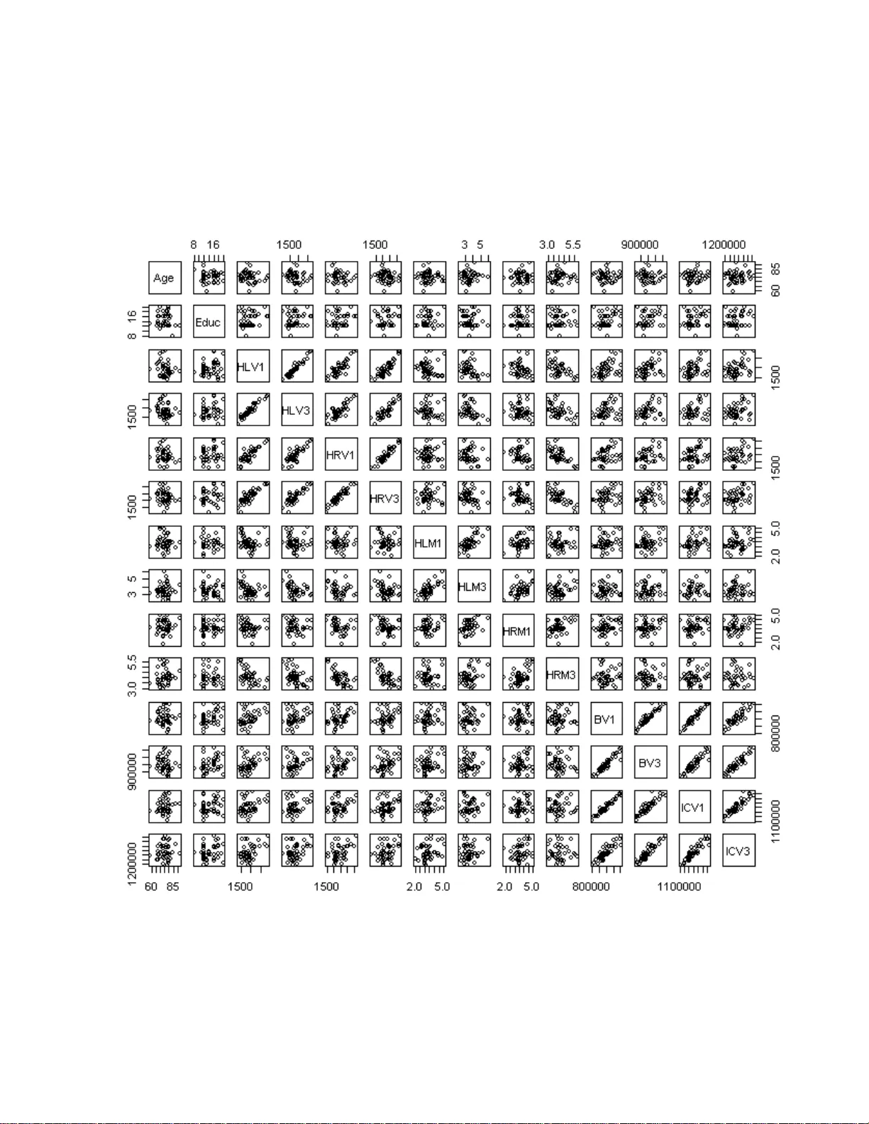
T ec hnical Rep ort # KU -EC-08-3: Analysis of Metric D istances and V olumes of Hipp o campi Indicates Diﬀeren t Morphometric Changes o v er Time in Demen tia o f Alzheimer T yp e a nd Nondemen ted Sub jects E. Ceyhan 1 , 2 ∗ , Can Cerito˜ glu 2 , M. F aisal Beg 3 , Lei W a ng 4 , John C. Morris 5 , 6 , John G. Csernansky 4 , 7 , Mic hael I. Miller 2 , 8 , John Tilak Ratnanather 2 , 8 Octob er 26, 2018 1 Dept. of Mathematics, Ko¸ c University, 344 50, Sarıyer, Istanbul, T u rkey . 2 Center for Imaging Scienc e, Th e Johns Hopkins University, Baltimor e, MD 21218. 3 Scho ol of Engine ering Scienc e, S i mon F r aser University, Burnaby, V5A 1S6, Canad a. 4 Dept. of Psychiatry, Washington University Scho ol of Me dicine, St . L ouis, MO 63110. 5 Dept. of Neur olo gy, Washington University Scho ol of Me dicine, St. L ouis, MO 63110 . 6 Alzh eimer’s Dise ase R ese ar ch Center, Washington University Scho ol of Me dicine, St.L ouis, MO 63110 . 7 Dept. of Anatomy & Neur obiolo gy, Washington University Scho ol of Me dicine, St.L ouis, MO 6311 0. 8 Institute for Computational Me dicine, The Johns Hopkins University, Baltimor e, MD 21218. * corresp onding author: Elv an Ceyhan, Dept. of Mathematics, Ko¸ c Univ ers ity , Rumelifeneri Y olu, 3 4450 S arıyer, Istanbul, T ur k ey e-mail: e lceyhan@ku.edu.tr phone: +90 (212) 338-1 845 fax: + 9 0 (212) 338-1559 short title: Metric distances b e t ween hippo campi predict shap e c hang es k eywords: morphometry , computational anatomy , Large Deformation Diﬀeomorphic Metric Mapping (LD- DMM), hipp ocampus, demen tia o f Alzheimer’s t yp e 1 Abstract In this a rticle, w e analyze the morphometry (shap e and size) of hipp ocampu s in sub jects with very mild dementia of Alzheimer’s type (DA T) and nondemented contro ls and how the morphometry changes ov er a tw o-year p eriod. Morphometric d i ﬀerences with resp ect to a template hipp ocampus were measured by the metric distance obtained from th e Large D ef ormation Diﬀeomorphic Metric Mapping (LDDMM) algorithm which was previously used to calculate dense one-to-one corresp ondence vector ﬁelds b etw een the shapes. LDDMM assigns metric distances on the space of anatomical images thereby allo wing for the direct comparison and quantization of morphometric changes. W e c h ara cterize what add i tional in- formation the metric distances provide in terms of size and shap e given the vol ume measurements of the hipp ocampi. Moreov er, we demonstrate ho w metric distances can b e used in cross-sectional , longitudinal, and left-right asymmetry comparisons. W e perform a p rincipal comp onen t analysis on metric distances and hipp ocampus, brain, and intracranial volumes. W e use rep eated measures A NO V A models to test the main eﬀects of and interacti on b et ween the diagnosis, du ra tion, and hemisph ere fa ctors to see which factors signiﬁcantly exp lain the diﬀerences in metric distances. When a factor is found to b e signiﬁcant, w e use classical parametri c and non-parametric tests to compare the metric distances for that factor. The analysis of metric distances is then used to compare the eﬀects of aging in the hipp ocampus. A t base- line, the metric distances for demented sub jects are found n o t to b e signiﬁcantly diﬀerent from those for nondemented sub jects. At fo llo w-up , the metric distances for demented sub jects w ere signiﬁcan t l y larger compared to nondemented sub jects. The metric d i stances for demen ted sub jects increased signiﬁcantly from baseline to follo w-up but not for nondemented sub jects. W e also d emo nstrate that metric distances can b e used in a logistic regression mo del for diagnostic discrimination of sub jects. W e compare metric distances with the volumes and obtain similar results in cross-sectional and longitudinal comparisons. In classiﬁcation, t he mod el that u ses vo lume, metric distance, and volume loss ov er time together p erforms b etter in detecting DA T. Thus, metric distances with respect t o a template comput ed v ia LDDMM can b e a pow erful t ool in detecting d iﬀerences in shape in cross-sectional as well as longitudinal stu dies. 1 In tro duction Numerous p ost-mortem studies hav e s ho wn that neuroﬁbrilla ry tangles and amyloid plaques characteristic of Alzheimer’s Disea se (AD) are pr ominen t within the hipp ocampus of individuals with mild dementia of the Alzheimer’s t y p e (D A T) and that the distribution of these ne ur opathological markers b ecomes mor e widespread to include sev era l regions o f the neo cortex as the disease pro cess prog resses [1-7]. The accum ula tion of neuroﬁbr illary tangles and amyloid plaques characteristic of AD are asso ciated with neuro nal damage and death [8]. F urthermore, macros c o pic gray matter losses from the accumulation of micr oscopic scale neuronal destruction ar e detectable in living sub jects using cur ren tly av ailable magnetic res o nance (MR) imaging. Spec iﬁc a lly , volume lo sses within th e hippo campus [9-1 4] hav e recen tly b een repor ted in sub jects with m ild-to- mo derate A D. In an un usual study where the ant emortem MR scans and p ost-mortem material was av a ilable for the same sub jects, hippo campal volume los ses were shown to be p ow erful antemortem predicto r s of AD neuropatholo g y [15]. P rogressive atrophy of the entire brain has b een observed in AD cases [1 6]. How ever, due to the complexity o f the human brain and the non-uniform distribution of AD neuropatholo g y ea rly in the course o f disease, detailed ex amination o f sp eciﬁc brain regions known to b e aﬀected early in the AD disease process (e.g., hippo campus) ma y be preferred for distinguishing preclinical and very mild forms of AD from normal aging [17- 19]. Metho ds developed in the ﬁeld o f Computational Anatom y (CA) that enable quan tiﬁcatio n of bra in struc- ture volumes a nd shap es b et ween and within gro ups of individuals with and without v arious neurolog ic al diseases hav e emerged fro m several groups in recent years [20-25]. Based on the mathematical principles of general pattern theor y [18 , 19, 23, 26 , 27 ], these metho ds c om bine imag e-based diﬀeomorphic maps betw ee n MR scans with repr e sen tations of bra in s tructures as smo oth manifolds. Because of their high rep eatabilit y and sensitivity to changes in neur o anatomical shap es, they can b e es pecially sensitive to abnormalities of brain structures asso ciated with early for ms o f AD. Using such metho ds, we previously demonstrated that the combined asses s men t of hippo campal volume los s and shap e defor mit y optimally distinguished sub jects with very mild DA T from b oth elder nondemented sub jects and younger healthy sub jects [10 ]. These metho ds also allowed us to demonstr a te that hippo campal shap e deformities ass ociated with very mild DA T and non- dement ed a ging were distinct [28]. These methods were also e xtended to quan tify c hang es in neur oanatomical volumes and sha pes within the same individua ls over time [29]. Other lo ngitudinal neuroimag ing analysis of hippo campal str uctures in individuals with AD have also emerged [30- 41]. 2 An imp ortan t tas k in CA is the s tudy of neuroanatomical v ariability . The anato mic mo del is a qua druple (Ω , G , I , P ) co ns isting of Ω the template co ordinate spa ce (in R 3 ), deﬁned as the unio n of 0, 1, 2, and 3- dimensional manifolds, G : Ω ↔ Ω a set of diﬀeomorphic tra ns f ormations on Ω, I the space of anatomies is the orbit of a template anatomy I 0 under G , and P the family o f pr obabilit y measures on G . In this framework, a geo desic φ : [0 , 1] → G is computed where each point φ t ∈ G , t ∈ [0 , 1] is a diﬀeomorphism of the do main Ω. The e volution of the template image I 0 along path is g iv en b y φ t I 0 = I 0 ◦ φ − 1 t such that the end po in t of the geo desic connects the template I 0 to the target I 1 via I 1 = φ 1 I 0 = I 0 ◦ φ − 1 1 . Th us, a natomical v aria bilit y in the target is enco ded by these geo desic tr a nsformations when a template is ﬁxe d. F urthermore, g e odesic cur v es induce metric distances betw een the template and the targ e t shap es in the orbit as follows. The diﬀeomor phisms a re constructed as a ﬂo w of or dinary diﬀerential equations ˙ φ t = v t ( φ t ), t ∈ [0 , 1 ] w ith φ 0 = i d the identit y map, and asso ciated vector ﬁelds, v t , t ∈ [0 , 1]. The optimal velocity vector ﬁeld para meterizing the geo desic pa th is found by solv ing b v = arg inf v : φ = R 1 0 v t ( φ t ) dt, φ 0 = id Z 1 0 k v t k 2 V dt such that I 0 ◦ φ − 1 1 = I 1 , (1) where v t ∈ V , the Hilber t space of smoo th v ecto r ﬁelds with no rm k·k V deﬁned thr ough a diﬀerential op erator enforcing smo othness. The length of the minimal length path through the space of transforma tions c o nnecting the given anatomical conﬁgurations in I 0 and I 1 deﬁnes a metric dista nce b et ween a natomical shap es in I 0 and I 1 via d ( I 0 , I 1 ) = Z 1 0 k b v t k V dt, (2) where b v t is the optimizer c alculated fr o m the Large Deformatio n Diﬀeomorphic Metric Ma pping (LDDMM) algorithm [42]. Here, the metric distance do es not hav e any units. The constructio n of such a metric spac e allows one to quant ify similarities and diﬀere nces b et ween anatomica l shap es in the orbit. This is the vis ion laid out by D’Arcy W. Thompson a lmost one hundred years ago . Figure 1 exempliﬁes the change in the metric distance during the ev olution of the diﬀeomorphic map fr om the template sha pe to the targ et shap e. The notion of mathematical biomarker in the for m of metric distance can be used in diﬀeren t ways. One is to g e ne r ate metric dista nces of sha p es relative to a template [42, 43]. Another is to genera te metric distances b et w een each shap e within a collection [44]. The la tt er appr oac h allows for sophis ticated pattern classiﬁcation analysis; it is how ever co mput ationally e x pensive. W e present an a na lysis ba sed o n the former approach whic h co uld provide a p o werful tool in analy zing subtle sha p e changes ov er time with considera bly less co mput ational load. This approach ma y allow detecting the subtle morphometric c hang es observed in the hippo campus in D A T sub jects in pa rticular for thos e pr eviously ana lyzed [29 , 45]. These studies co mp ared rates of change in hippo campal volume and shap e in sub jects with very mild DA T and matched (for age and gender) nondemented sub jects. The change in hipp oc ampal shap e over time was deﬁned as a residual vector ﬁeld resulting from rig id- bo dy motion registr ation, and c ha nges in patterns along hipp oca mpal surfaces were visualized and ana lyzed via a statistical measure o f individual and gro up ch ange in hippo campal shap e ov er time and used to distinguish b et ween the sub ject groups. Hence the motiv ation to analyze LDDMM generated metric distances b et ween bina ry hipp oca mpu s images at baseline a nd at follow-up with resp ect to the sa me template hipp o campus image. That is, the template was compar e d aga in, and no t pr o pagated betw een time points. One migh t wonder why we do not track changes within a sub ject directly , ra th er than via a r eference template, as it could give a more sensitive measure of shap e change s inc e the small diﬀerence in shap e would make ﬁnding co rrespo ndence more accurate. Although w e hav e considered doing this, the diﬃcult y is that s ince the template (or orig in) is diﬀeren t for each lo ng itudinal co mp utation, how to corr ectly per form statistical compar ison o f group c ha ng e is not completely settled. This is a c tively b eing dev elop ed b y using the concept of “para llel transp ort” [46, 4 7]. In this study , we co mpute and a na lyze metric distances based on the data used in [2 9]. W e brieﬂy describe t he data set in Section 2.1, computation of metric distances via LDDMM in S ection 2.2, statistical metho ds we employ in Section 2.3 , and results a nd ﬁndings in Section 3, which include descriptive summary s tatistics of the metric distances, compariso n of metric distances of hipp oc ampi of non-demented sub jects and sub jects with very mild dementia, corr elation b et ween metric distances, co mparison of distri- butions o f metric distances, and disc r iminativ e p o wer of metric distances. W e p erform similar a nalysis on hippo campal v o lumes in Se c tio n 4, compare v olumes and LDDMM distances in Section 5, and analyze ann ual 3 per cen tage r ate of change in volumes and distances in Section 6. In the ﬁna l section, we discuss the use of metric distances for ba seline-follo wup studies, g roup comparisons , and discr imina tion analysis. 2 Metho ds 2.1 Sub jects and Data Acquisition Detailed description of sub jects can b e found in [29] where 18 very mild DA T sub jects (Clinical Dementia Rating Scale, CDR0.5) and 26 age -matc hed nondemented con trols (CDR0) were each scanned a ppr o ximately t wo y e ars apar t. Clinical Dementia Rating (CDR) Scale ass essmen ts which detect the severity of demen tia symptoms were p erformed a nn ually in all sub jects by exp erienced clinicia ns without reference to neuro psy- chological tests or in-v ivo neuroima g ing d ata. The ex perienced clinician conducted semi-str uctured in terviews with an informant and the sub ject to asse s s the s ub ject’s c o gnitiv e and functional p erformance; a neurolo gi- cal examination was also o btained. The clinician determined the presenc e o r absence of demen tia a nd, when present, its s ev erity with the CDR. Overall CDR scores of 0 indicate no dementia, while CDR sc ores of 0.5, 1, 2, and 3 indica te v er y mild, mild, mo derate and s ev ere dementia, resp ectively [48]. CDR asses smen ts hav e bee n s ho wn to hav e a n inter-rater reliability of κ = 0 . 74 (w eighted k appa co eﬃcien t [49] κ of 0 .87) [5 0], a nd this high degr e e of inter-rater r eliabilit y has b een conﬁrmed in multi-cen ter dementia s tudies [51]. Elderly sub jects with no clinical evidence of dementia (i.e., CDR0 sub ject) hav e b een conﬁrmed with nor ma l bra ins at autopsy with 8 0% accur a cy; i.e., approximately 20% o f such individuals show evidence of AD [52]. CDR0.5 sub jects have s ubt le cog nitiv e impa irmen t, and 93% of them progres s to mo re severe stage s of illness (i.e., CDR > 0.5 ) and show neuropatho logical signs of AD at autopsy ([53], [54], and [52]). Although elsewhere the CDR0.5 individuals in our sample may b e co nsidered to have MCI [5 5], they fulﬁll our diagno s tic criter ia for very mild D A T and at a utopsy ov er whelmingly have neuropatholog ic AD [56]. A summary of sub ject information is listed in T able 1 . The scans were obtained using a Magnetom SP-4 0 00 1.5 T esla ima g ing system, a s tandard head coil, and a magnetization prepared r apid gradie nt echo (MPRAGE) sequenc e . The MPRAGE sequence (TR/TE - 10/4 , A CQ - 1, Matrix - 256 × 2 56, Scanning time - 11.0 min) pro duced 3D data with a 1 mm × 1 mm in-plane resolution and 1 mm slice thickness acros s the entire cr anium. A neuroanato mical template was pro duced using an MR image from an a ddit ional elder control (i.e., CDR0 o r non- demen ted) s ub ject (male, age = 69 ). The c ho ice and a detailed de s cription o f the template is provided in [57]. The sub ject selected to pr oduce this template was obtained from the same sour c e as the other sub jects in the study , but was not o therwise included in the da ta analysis. Data used ar e the left and right hippo campal surface s in the template scan cr eated f rom ex pert-pro duced manual outlines using metho ds previously describ ed [28,5 8], and the left and right hippo campal surfa ces of e a c h s ub ject gener a ted at ba s eline and follow-up. These surfa c e s were conv er ted to binary hippo campus volumetric images b y ﬂo od ﬁlling the inside of the surface and g iv ing it lab el 1, and the outside of the surfac e was lab eled as 0, o r bac kg round. Each individual hipp oca mpa l surfac e was ﬁrst scaled by a factor of 2 and aligned with the template surface, which was a ls o sca led by a facto r o f 2 , v ia a rigid- bo dy r o tation a nd tr anslation b efore co n verting to volumetric binary imag es. In [58] we showed that mapping accuracy could b e enhanced at higher resolution beca use of smaller vo xels – vo xels at the p eriphery of the structur e (i.e., surfa c e) account for muc h mo r e of the structural volume at 1 mm 3 vo xel res olution versus 0 . 5 mm 3 . Since then we hav e ada pt ed this as part of the standar d mapping pr ocedure. These surfaces were then conv erted into binarized image of dimension 64 × 11 2 × 64 with v oxel reso lutio ns of 0 . 5 × 0 . 5 × 0 . 5 mm 3 , followed by smo othing by a Gaussia n ﬁlter of 9 × 9 × 9-voxel window and o ne vo xel standar d deviatio n to smo oth out the edge s for LDDMM, whic h was then a pplied to each template- sub ject pa ir to compute metric distances, d b k , d f k ( k = 1 , . . . , 44 ), in each hemisphere at baseline ( b ) and at follow-up ( f ) as illustr a ted in Figur e 2. Controlling for bra in size is impo rtan t b ecause pe o ple with bigger brains tend to hav e bigger hipp oca mpus and we wan t our results to no t reﬂect that very uninteresting fact; we inherently cor r ect for brain size by ﬁrs t rigid-alig ning the sub ject br ain to the proto t yp e brain prio r to LDDMM. Segmentation o f hipp ocampal MRI shap es a c ross sub jects, esp ecially in disease d s ta tes, is a challenging pr oblem. How ever the accuracy of the segmentation is not the point of this pap er and has b een demonstrated b efore [10, 5 7, 58]. 4 In addition to the metric distances, our data set also consis ts o f the following v ar iables: g ender, age, educa- tion in years (these v ariables a re use d for controlling the c o nfounding aﬀects of thes e factors on hipp ocampus morphometry , so the s ub jects a re taken to be s imilar or evenly distributed in these v ar iables). F urther mo re, we hav e brain and intracrania l volumes at bas e line and followup, and hipp o c a mpus volumes for left and rig h t hippo campi at baseline and fo llo w-up. 2.2 Computing Metric Dist a nce via Large Deformation Diﬀeomorphic Metr ic Mapping Metric distances b et ween the binary image s a nd the template image are obtained by computing diﬀeomor - phisms b et ween the images. Co mpu tation and a nalysis of these diﬀeomo rphic mapping s hav e b een pr eviously describ ed [57]. Diﬀeomorphisms are estimated via the v ar iational problem that, in the space of s mooth velocity vector ﬁelds V on doma in Ω, ta k es the for m [4 2]: b v = arg min v : ˙ φ t = v t ( φ t )  Z 1 0 k v t k 2 V dt + 1 σ 2   I 0 ◦ φ − 1 1 − I 1   2 L 2  . (3) The optimizer of this c o st gener ates the optimal change o f co ordinates ϕ = φ b v 1 upo n integration d b φ v t  dt = b v t  b φ v t  , φ 0 = id , wher e the subscript v in φ v is used to explicitly denote the dep endence of φ on the asso ciated velocity ﬁeld v . Enforc ing a s uﬃcie nt amount o f s mo othness on the elements of the space V of allow able velocity vector ﬁelds ens ures that the solution to the diﬀere ntial equatio n ˙ φ t = v t ( φ t ) , t ∈ [0 , 1] , v t ∈ V is in the space of diﬀeomorphisms [59 , 6 0]. The required smo othness is enforced by deﬁning the norm o n the space V of smo oth velo cit y v ector ﬁelds through a diﬀerential o perator L of the t y pe L = ( − α ∆ + γ ) α I n × n where α > 1 . 5 in 3-dimensiona l space such that k f k V = k L f k L 2 and k·k L 2 is the standar d L 2 norm for squa re int egrable functions deﬁned on Ω. The g r adien t of this cos t is given by ∇ v E t = 2 b v t − K  2 σ 2    D φ b v t, 1    ∇ J 0 t ( J 0 t − J 1 t )  (4) where J 0 t = I 0 ◦ φ t and J 1 t = I 1 ◦ φ − 1 t , | D g | is the determinant of the Jacobian matrix for g a nd K is a compact self-adjoint op erator K : L 2  Ω , R d  → V uniquely deﬁned by < a, b > L 2 = < K a, b > V such that for any smo oth vector ﬁeld f ∈ V , K ( L † L ) f = f holds. The metric distance is then calcula ted via Equatio n (2). 2.3 Statistical Metho ds First, we inv estiga te wha t LDDMM metr ic dis ta nce measures and how it is related to hippo campus, brain, and intracranial volumes. Tha t is, as a comp ound mea s ure of mo rphometry , how muc h of the metric distance is related to sha p e and size a nd ho w it is asso ciated with the volume, which is mostly a meas ur e of s iz e. Along this line, w e pro vide the corr e la tion b et w een v olume and metr ic distance measures b y the pairs plots at base line and follow-up o f left a nd right hipp oc ampi. F urthermor e, we p erform a principa l comp onent a nalysis (PCA) on metr ic distance and volumes to c ha racterize the ma jor traits thes e q uan tities measure. Then we provide a statistical metho dology for the analysis of LDDMM distances. W e compute and interpret simple summary statistics, such as, mean, sta ndard de v iation (SD), minimum, ﬁrst quartile ( Q 1 ), median, third quartile ( Q 3 ), and maximum for d { b,f } k . Then we apply rep eated measures analys is of metric dis ta nces with diagnosis group as main eﬀect and timep oin t as the r epeated fac to r, side (i.e., hemisphere) a s main eﬀect and timepo in t as the r epeated factor, and diagnosis group as ma in eﬀect and side-by-timepo in t as the rep eated facto r, since there are within-sub ject dep endence o f metric distances for left and right hemispheres and at baseline and follow-up. W e a pply four p ossible comp eting mo dels ea c h assuming a diﬀerent v ariance-c o v aria nce structure to obtain the mo del that b est ﬁt to our data set. The ﬁr s t mo del assumes comp ound s ymmetry , in which the diagonals (i.e., the v a riances) are equal, and so ar e the oﬀ diag onals (i.e., the cov aria nces). The other three mo dels ass ume uns tructured, auto r egressive (AR), and autoregr essiv e hetero geneous v ariances , resp ectively . In the unstructured mo del, each v aria nce a nd cov ariance term is diﬀerent, in the AR mo del, the v aria nces are a ssumed to b e equal but the cov ariances c hange by time, a nd in the ARH mo del, the v a riances are also diﬀerent and the cov a r iances change by time. The co rrespo nding v ariance-cov ariance (V ar - Co v) structures 5 [61-63 ] for the mo dels ar e shown in T able 5, wher e σ 2 is the commo n v ariance term, σ 2 i is the v ariance for rep eated factor i , σ ij is the cov ariance b et w een rep eated factor s i and j , and ρ is the c orrelation co eﬃcien t of ﬁrst order in an autor egressive mo del. W e use v ario us mo del selection criteria (Ak aike Info r mation Cr iterion (AIC), Bay esian Informatio n Criter ion (BIC), Lo g-lik e liho o d) to compare c ompeting mo dels to see which mo del b est ﬁts our data [64 ]. F or p ost-ho c co mpa rison of CDR0.5 vs CDR0, our null hyp o thesis fo r the compariso n of diag nosis groups, CDR0 and CDR0.5, is H o : µ C D R 0 = µ C D R 0 . 5 for each baseline left, baseline r igh t, a nd follow-up left, follow- up right hipp oca mpi. F o r the t -test, amo ng the underly ing assumptions ar e the nor malit y of the dis tr ibutions and homog eneit y of the v aria nces of the indep enden t samples. W e employ Lilliefor’s tes t of norma lit y [65]; and Brown and F orsythe’s (B-F) test (i.e., Lev ene’s test with a bsolute devia tio ns from the median) for homogeneity of the v ariances [66 ]. If there is lack of signiﬁcant deviation fr om nor malit y o f distribution of a metric distances for a gr oup, we will state it a s “the metric distances for the group can b e ass um ed to co me from a normally distributed popula tion”, henceforth. W e compare metr ic distances at bas e line and follow-up. The LB -CDR0.5 metric distances and L F- CD R0.5 metric distances are dep enden t as they come from the same p erson at baseline and fo llo w-up. Likewise for LB-CDR0 and LF-CDR0 pairs. Hence our null h ypo thesis for the comparis on o f baseline and follow-up groups is H o : δ ( B , F ) = 0 wher e δ ( B , F ) is the mean diﬀerence of metric distances b et ween hipp oc ampi at baseline and follow-up for e a c h of CDR0 left, CDR0 r ig h t, CDR0.5 left, CDR0.5 right hipp ocampi. W e also co mpare the metric distances for the left and rig h t hipp ocampi are dep enden t (for each left-right hipp ocampi pa ir comes fr o m the same sub ject). Hence o ur n ull hypo thesis for the compar ison of left a nd right metric distances is H o : δ ( L, R ) = 0 where δ ( L, R ) is the mean diﬀerence o f metric distanc e s b et ween left a nd right metric distances for each of CDR0 ba seline, CDR0 follow-up, CDR0.5 baseline, CDR0.5 follow-up hipp oca mpi. W e also calcula te and interpret cor relation co eﬃcien ts b et ween metric distances. Since metric distances of all groups can b e assumed to hav e normal distr ibution based o n Lilliefor’s test of nor ma lit y , we use Pearson’s correla tion co eﬃcient , denoted r P , b et ween ba seline and follow-up (o verall and by dia gnosis group) and for the left a nd r igh t hippo campi and the corres p onding tests of H o : r P = 0 vs H a : r P > 0 for inference [67,68]. W e also estimate the empirical c umulative distr ibut ion functions (cdf ) of the metric distances and compare them by Kolmog oro v-Smirnov (K-S) test, Cr am ´ er’s test, and Cra m ´ er-von Mises test. The null hypo thesis for the compariso n of cdfs of the metr ic distances p er diagno sis groups, CDR0 and CDR0.5, is H o : F C D R 0 = F C D R 0 . 5 for ea ch baseline left, baseline right, follow-up left, follow-up right hippo campi. F or calcula tio n of the critical v alue of Cr a m ´ er’s test the kernel φ C ( x ) = √ x 2 (whic h is r ecommended for lo cation alter nativ es) is used. The estimated p -v alues ar e based on α = 0 . 05 and 10 0 00 or dinary b ootstrap r e plicates. W e a pply log istic discrimina tion with metric dis tances a nd other v ariables , since the diagno s is hav e only t wo lev els, na mely CDR0 and CDR0.5. W e use lo g istic regression to e s timate or predict the risk o r probabilit y of having D A T using metric distances, tog ether with side (i.e., hemisphere) a nd timepo in t (baseline vs follow- up) factors. In other words, we mo del the probability tha t the sub ject is CDR0.5 given the metric distance of the sub ject for left o r right hippo campus at baseline or follow-up. In s ta ndard logis tic regres sion the mo del-parameters ar e obtained via maximum likelihoo d es tim ators. F or more on lo gistic regres sion and logistic discrimination, see [69] and [70], res pectively . W e cons ider the logistic mo del with the res ponse where (i.e., the pr obabilit y that the sub ject is diagnosed with CDR0.5). First we model with one predictor v ariable at a time fro m side, timep oin t, and metric distance, etc., if the v a riable is not signiﬁcant at .05 level, we omit that v ariable from further co nsideration. W e consider the full logistic mo del with the resp onse logit p = log [ p /(1 − p )] where p = P ( Y = 1 ) ( i.e., the proba bilit y that the sub ject is diagnos e d with CDR0.5 ); the remaining v a riables with all p ossible interactions as the predic to r v aria ble s . On this full mo del, we cho ose a reduced mo del by AIC in a stepwise algor ith m, and then us e stepwise backward elimination pro cedure on the re s ulting mo del [64 ]. W e stop the elimination pro cedure whe n all the remaining v ariables are signiﬁcant at α = 0 . 0 5 level. Based o n the ﬁnal mo del with sig niﬁcan t predictor s, we apply log istic discrimination. In logistic discr imi- nation the log -odds-r a tio of the conditional cla ssiﬁcation and ther efore indirectly the conditional pr o babilities of be ing CDR0.5 a nd CDR0 are mo deled. In g eneral, if this estimated pro babilit y is larger than a pr especiﬁed probability p o , the sub ject is classiﬁed as CDR0.5, otherwis e the sub ject is classiﬁed as CDR0 (i.e., nor ma l). 6 This means our decis ion function reduces to b p k = P ( Y = 1 | d ij k )  > p o ⇒ classify C DR 0 . 5 , ≤ p o ⇒ classify C DR 0 , (5) where p o is usually taken to be 0.5 . This threshold pro babilit y p o can also b e optimized with resp ect to a cost function which inco rpora tes cor rect cla ssiﬁcation rates, sens itivit y , and/or sp eciﬁcit y [71]. W e apply the same analysis pro cedure on hipp oca mpal volumes to co mpare the results with LDDMM metric dis tances. F urthermore, w e ﬁnd the diﬀerent ial v olume lo ss a nd metric distance change by using the annual p ercen ta ge rate of change (APC) in v olume and metric distance (see [71 ] for APC in volume for ent orhinal cor tex). W e a lso co nsider the log istic discr imination mo dels that incorp orate volume and metric distance together and APC in volumes a nd metric distances tog ether. 3 Analysis of LDDMM Distances of Hipp o campi 3.1 Preliminary Analysis of LDDMM Distances and Other V ariables The summary mea sures for the v ariables are provided in T able 1. Observe that the sub jects are ev enly distributed in terms of gender, y ears of education, scan interv a ls , and age for the diagnos tic gro ups. The brain and in tracrania l volumes are m uch larger in sca le, then come the hippo campal volumes, and then the metric distances. Notice that brain and hipp o campal volumes all decreas e b y time and are smaller in CDR0.5 sub jects compar ed to CDR0 s ub jects. On the o ther hand, the metric distances tend to increase by time and are larg er for the CDR0.5 sub jects. Also pres e nted in T able 1 are the p - v alues for Lilliefor’s test o f norma lity and Wilcoxon rank sum tes t for diﬀerences betw een the diagnostic groups. Notice that most v ariables can be a ssumed to follow a Gaus s ian distributio n, but since a few fails to do so, w e apply the Wilcoxon rank sum test instea d o f W elch’s t - test. The dia g nostic gro ups do not signiﬁcantly diﬀer in a ge, education, bra in and intracranial volumes. F urther mo re, among the metric distances, we see that only right follow-up metr ic distances are sig niﬁca n tly diﬀere nt b et ween the diagnostic g roups. W e present the pair s plot (sca tter plot o f each pair) of c on tinuous v ar ia bles in Figure 3 and als o calculate the cor relation co eﬃcien ts betw een ea c h pair of the v a riables (not pr esen ted). W e observe that age and education a re not signiﬁca n tly co rrelated with any of the other v a riables. Hence we discar d them in our prosp ectiv e analys is (except for logis tic discrimination). W e observe signiﬁcant cor relation b et ween each pair of hipp ocampa l volumes, and betw een each pair of br a in and in tr a cranial volumes. The metric distances are o nly mo derately cor related with each other . Hipp ocampal v olumes ar e mildly co rrelated with brain a nd int racrania l volumes. The same holds for the metric distances but to a le s ser extent. Summary statistics of p opulation mea n, standar d deviation (SD), minimum, ﬁrst quartile ( Q 1 ), median, third quartile ( Q 3 ), and maximum for d { b,f } k are pr esen ted in T a ble 1. Baseline metric distances s eem to b e diﬀer en t in distribution (lo cation and spread) fr o m follow-up metr ic distances follow-up dista nces b eing larg er than baseline distances for b oth left a nd rig h t hipp oca mpi; likewise left metric dista nces seem to be diﬀerent from r ig h t metric dista nces with r igh t distances b eing larger than left for bo th ba s eline and follow-up. Let LDB b e the metr ic distances for left hipp oca mpi at baseline, LDF be the metric distances for left hippo campi at follow-up. Let RDB and RDF be similar ly deﬁned for rig h t hippo campi. O ne - tailed t -tests revealed tha t the or der of these meas ur es is LDB < LDF < RDB < RDF with all inequalities b eing signiﬁca n t at .05 level. This implies that the mo rphometric diﬀerences of left hipp oca mpi with res pect to the left hipp o c ampus of the template sub ject a t ba seline a re signiﬁcantly sma ller than those at follow-up, i.e., at base line, left hipp ocampi are more similar to the left template hipp ocampus, and by follow-up le ft hippo campi tend to be c o me more diﬀerent in morpho metr y (shap e and size) from the template hippo campus. This is not surprising , as the template hippo campus is one from the baseline hipp oca mpi. Tha t is the template was based on a ba s eline scan. Although this should seem to b e irrelev ant in v iew of the wide age v a riation, it is not the age that is the main p oin t here, when base line a nd follow-up ar e compar ed, we use matched pair (i.e., dep enden t) tests, which would r ev eal diﬀere nce s that would o ther wise b e co ncealed by the independent t wo-sample tes ts. F o r example, when all the sub jects age abo ut tw o y ears, their morpho metric alterations accumulate to render their relative diﬀere nce from the template more signiﬁcant. 7 The rig h t hipp o campi reveal s imila r mor phometric diﬀerences and change ov er time. F urthermor e, we observe that the mor phometric diﬀerence of right hipp ocampi fro m the r igh t template hipp oca mpus is sig- niﬁcantly lar ger compa r ed to the morpho metric diﬀerence o f left hipp oc a mpi fr om the left template at both baseline and follow-up. The summary statistics (means and sta nda rd deviations (SD)) for left and right metric distances by g r oup a re provided in T a ble 1. Observe that CDR0 distances a r e smaller tha n CDR0.5 dista nc e s at baseline and at follow-up for bo th left and right hipp o c ampi. This sugges ts tha t the morphometric diﬀerences of CDR0 hipp oca mpi with r espect to the template hipp oca mpus are smaller than those of CDR0.5 hipp ocampi. This is not surprising, consider ing the template hipp oca mpu s being o ne of the CDR0 hipp ocampi. F urthermor e, the standar d deviations of the distances for CDR0 sub jects tend to b e smaller than those of CDR0.5 sub jects. That is, the morphometric v ariability of CDR0 hipp oc a mpi with re s pect to the template hipp oc ampus is smaller than that of CDR0.5 hippo campi. The statistical signiﬁca nce of these res ult s will b e provided in the following sections. See also Figure 4 for the (jittered) scatter plots of the metric distances by gro up, where the cro sses are centered at the mean distances and the points a re jittered (scattered) along the horizontal axis in or der to a void frequent p o in t concur rence and tight clustering o f p oin ts, thereby mak ing the plot b etter for visualiz a tion. 3.2 Principal Comp onen t Analysis for the V olumes and Metric Distances The volumes and metric distances measur e diﬀerent but rela ted asp ects of mo r phometry , so some of the v ariables a r e hig hly corr elated with each other (see Figur e 3). W e p erform principal co mponent a nalysis (PCA) to obtain a set of uncor r elated v a riables that hopefully r epresen t so me identiﬁable asp ect of the morphometry . See [7 0,76] for more o n PCA. When we p erform PCA of metric distances and volumes of left hippo campi at baseline with eigenv alues ba sed on the cov ar iance matr ix, we obser v e tha t the ﬁrst principal comp onen t (PC) acco un ts for almost all the v a riation (see T able 2). Considering the v ariable loadings in T able 2, we see that PC1 is the head siz e comp onent , PC2 is the contrast b et ween brain a nd intracranial volumes, P C3 is the hipp ocampus siz e , and P C4 is the metric distance comp onent. Ho wev er, the volumes are in mm 3 and metric distance s are unitless, hence the data are not to scale. In particular, the brain and int racrania l volumes hav e the largest v a riation in the data set, hence domina te the PCs. T o remove the inﬂuence o f the scale (or unit), we a pply P CA with eig en v alues based on the cor r elation matrix (i.e., P CA on the standar diz e d v ariable s ). The imp ortance scores of principal comp onents and v aria ble loading s from the PCA of metric dista nces and volumes of le f t hipp oca mpi at baseline and followup with eigenv a lues bas ed on the co r relation matrix are presented in T able 3. Notice that with the cor r elation matrix, the ﬁrst three PCs account for almos t all the v ariation in the v ariables. Compar ing the v ar iable lo adings, PC1 se ems to b e the head size comp onen t, P C2 is the hippo campus shap e, P C 3 is the hippo campus size and the contrast b et ween hippo campus a nd head size , and PC4 is the contrast b et ween brain a nd intracranial volume. The PCA on v ariables for right hipp ocampi yields similar results (see T a ble 4). The v ar iable lo adings in the PCA o f v ariables a t ba seline and follow-up sugg est that brain a nd intracra- nial volumes are mostly measur es of head size, metric distanc e is mostly a measure of hippo campus shap e and par tly is a measure of head a nd hipp oca mpu s size, and hippo campus volume is mos tly a measur e of hippo campus size a nd pa rtly r elated to hipp ocampus shap e and head s ize. Tha t is, volumes and the metric distance co nvey information that is rela ted but not identical. V olumes mostly emphasize the size diﬀere nce s, while metr ic distance s emphasize the sha p e diﬀerences. Hence, one sho uld us e b oth of them in morphometr ic analysis of bra in tissues . 3.3 Rep eated Measures A nalysis of LDDMM Distances Due to within-s ub ject dependence of metric dis tances for left and rig h t hemispheres a nd for baseline a nd follow-up mea sures, we apply rep eated-measures a nalysis with group and side as main eﬀects and timep oin t as the rep eated factor, and gr oup a s main eﬀect a nd side-by-timepo in t as the rep eated fa c tor (see be lo w). F or the left data, metric distances a t baseline for CDR0.5 sub jects are lab eled as LB-C DR0.5 , at follow-up are lab eled as L F- CDR 0.5. CDR0 individuals a re la beled as LB-CDR0 and L F-CDR0 accor ding ly . Similar lab eling is done for the righ t metric distances . Hence, we have four measur emen ts for each sub ject, so rep eated measures analysis ca n b e p erformed o n o ur data set. 8 3.3.1 Mo deling LDDMM Distances with Group as M ain Eﬀe c t wi th Comp ound Symmetry in V ar-Co v Structure F or the rep e ated measur es ANOV A with group as main eﬀect a nd comp ound symmetry r epeated over time, for each sub ject, we will denote diagnosis , timepoint, a nd hemisphere factor s a s numerical subsc ripts for conv enience. The co rrespo nding mo del is d ij k = µ + α D i + α T j + α DT ij + ε ij k (6) where d ij k is the distance for sub ject k with diagnosis i ( i = 1 for CDR0; 2 for CDR0.5) at timep oin t j ( j = 1 for base line; 2 for follow-up), µ is the overall mean, α D i is the eﬀect o f diagnos is level i , α T j is the eﬀect of timep oin t level j , α DT ij is the diagnos is-b y-timep oint in teraction, i.e., part of the mean dis ta nce not a ttributable to the additive eﬀect o f diag nosis and timep oin t, and ε ij k is the err or term. The V ar-Cov structure for the er r or term is V ar ( ε ij k ) = σ 2 and Co v ( ε ij k , ε ij ′ k ) = σ T 1 . Notice that the eﬀect of side (left or right) is ignor ed in this mo del. There is no signiﬁcant gr oup main eﬀect ( F = 3 . 36 , d f = 1 , 42 , p = 0 . 0 739). Ho wev er, the within group time-p oin t main eﬀect ( F = 11 . 16 , d f = 1 , 130 , p = 0 . 001 1 ) and the gro up-b y-timep oin t in teraction ( F = 4 . 8 4 , d f = 1 , 13 0 , p = 0 . 0295) a re b oth signiﬁcant, which imply that the tw o gro ups should b e c o mpared at the diﬀerent time p oin ts. In Figur e 5, we present the int eraction plots for diagno sis ov er time, where the end p oint s of the line seg men ts a r e lo cated at the mean metric distances at baseline and follow-up years. W e see that bo th lines increa se ov e r time, but are not para llel; the incr ease of the line for CDR0.5 g roup is steep er. 3.3.2 Mo deling LDDMM Distances with Si de as Main Eﬀect with Comp ound Symmetry i n V ar-Co v Structure F or the r epeated measures ANOV A with side as main eﬀect and comp ound symmetry rep eated over time, the corr esponding mo del is d ij k = µ + α S i + α T j + α S T ij + ε ij k (7) where d ij k is the dis ta nce for s ub ject k for side i ( i = 1 for left; 2 for right) at timepo in t j ( j = 1 for ba seline; 2 for follow-up), µ is the overall mean, α S i is the eﬀect of side level i , α T j is the eﬀect of timep oin t level j , α S T ij is the side-by-timepoint interaction, and ε ij k is the err or term. The V a r-Co v structure for the error ter m is V ar ( ε ij k ) = σ 2 and Co v ( ε ij k , ε ij ′ k ) = σ T 1 . Notice that the eﬀect o f diagno sis (CDR0 or CDR0.5) is igno red in this mo del. The side and timep oin t main eﬀects a re b oth signiﬁcant ( F = 20 . 2 5 , d f = 1 , 129 , p < 0 . 0001 and F = 12.51, df = 1 ,1 29, p = 0.0 006, re spec- tively), but side-by-timepoint interaction is not sig niﬁcan t (F = 1.85, df = 1,129 , p = 0.1 766). Conseq uen tly , we see that the lines ar e par a llel but far apa r t, the main eﬀect o f side co mparison is mea ning ful and a bout the same at each timepoint. Mor eo ver, the side s do change in mor phometry ov e r time. In Figure 5, w e see that b oth lines inc r ease ov er time a nd are parallel, but the slop e for right side s eems to b e steep er, which will even tually make the slop e estimates signiﬁcantly diﬀere n t. 3.3.3 Mo deling LDDMM Distances wi th Group, Si de, and Group-by-Side Intera ction Lo oking a t mo dels including only the main eﬀects of side or group separately does not answer all our questions. W e would also like to know, for example, if the metric distances of left hipp oca mpi o f CDR0.5 sub jects are diﬀerent from those of left CDR0 sub jects. In o rder to address these types of questio ns we need to lo ok a t a mo del that includes the interaction of diagnosis and side. First, we need to mo del the V ar -Co v structure for the rep eated measures for each sub ject. W e hav e fo ur cor related measur es p er sub ject, namely LDB, LDF, RDB, and RDF. Below is the estimated V ar- C ov matrix for these v ar iables:     0.46 0.35 0.1 8 0.0 2 0.35 0.60 0.2 4 0.1 8 0.18 0.24 0.4 5 0.2 3 0.02 0.18 0.2 3 0.4 4     9 W e s ta rt with co mpound s ymmetry for our mo del, and then try unstruc tur ed, autoregr essiv e (AR), and a u- toregre s siv e hetero geneous (ARH) V ar-Cov structur es. The v a riances (in the diag onal) sugg est hetero geneit y betw een them, a nd also, cov ariances s e em to diﬀer. This sugges ts that either an unstructured or ARH mo del might ﬁt this data bes t. See T able 6 for the compar ison o f mo del selection criteria s uc h as AIC, BIC, a nd Log-likeliho od and likeliho od ratio test p - v alue. The most promising model is the unstructured mo del based on lik e liho o d r atio test, since -2 Log Likelihoo d scores are signiﬁcantly sma ller than the -2 Log Likelihoo d scores of o ther mo dels. How ever, BIC and AIC f av or the model with the AR v ariance - co v ar iance str ucture. Besides, the log-likeliho od appro ac h gives the sec ond smallest -2 Log Likeliho od scor e for this mo del. Hence, we choose the mo del with AR V a r-Cov structure. The corr esponding mo del is d ij k l = µ + α S i + α D j + α T k + α S D ij + α S T ik + α DT j k + α S DT ij k + ε ij k l , (8) where d ij k l is the distance for s ub ject l for s ide i (1 for left; 2 for rig h t) with diagnosis j ( j = 1 for CDR0; 2 for CDR0.5) at timep oin t k ( k = 1 for ba seline; 2 for follow-up), µ is the ov er all mean, α S i is the eﬀect of side level i , α D j is the eﬀect o f dia gnosis level j , α T k is the eﬀect o f timep oint level k , α S D ij is the side-by-diagnosis int eraction, α S T ik is the side- b y-timep oin t interaction, α DT j k is the diag nosis-b y-timepo in t int eraction, α S DT ij k is the side-by-diagnosis-by-timepoint interaction, and ε ij k l is the error term. The V a r-Co v structure for the error term is Co v ( ε ij k l , ε i ′ j k ′ l ) =     σ 2 σ ρ σ 2 σ ρ 2 σ ρ σ 2 σ ρ 3 σ ρ 2 σ ρ σ 2     . The three way interaction of side-by-group-by-timepo in t is not signiﬁcant ( F = 0 . 5 0 , d f = 1 , 168 , p = 0 . 4 823), and neither ar e the tw o w ay side-by-group ( F = 0 . 76 , d f = 1 , 168 , p = 0 . 3860 ), a nd side- by-timep oin t int eractions ( F = 2 . 2 5 , d f = 1 , 168 , p = 0 . 135 9). O n the other hand, the gro up-b y-timep oin t interaction is sig niﬁcan t ( F = 8 . 47 , d f = 1 , 168 , p = 0 . 0 041). The main eﬀects o f s ide , group, and timepo in t a re a ll signiﬁcant ( F = 6 . 12 , d f = 1 , 168 , p = 0 . 01 43; F = 4 . 05 , d f = 1 , 168 , p = 0 . 04 57; and F = 19 . 52 , d f = 1 , 168 , p < 0 . 00 01, resp ectiv ely), but due to in ter action, the main eﬀect for diag no sis (i.e., group) is close to clinically mea ningless; i.e., the gr oups should b e compare d a t each t ime p oint instead o f an ov er all co mparison of group means . But, the main eﬀects of timepo in t and side b eing sig niﬁcan t is int erpretable b et ween baseline and follow-up. Below we p erform v arious p ost-hoc tests to s ee which gr oups are sig niﬁcan tly diﬀerent or sig niﬁcan tly change over time. T o acco mplis h this, we test fo r diﬀerence s a t each timep oin t, b et ween ba seline a nd fo llo w- up, and b et ween left a nd rig h t distances. 3.4 P ost -Hoc Comparison of LDDMM Distances of CDR0.5 vs CDR0 Hip- p ocampi F or the p -v a lue s r egarding the compar is on o f independent groups, see T a ble 7. The s ig niﬁcan t v alues at α = 0 . 05 ar e marked with *. None of the dis tance g roups devia te signiﬁca n tly from normality (all p -v alues grea ter than 0.1 0 ). That is , distance dis tr ibution of each group ca n be assumed to come from a Ga ussian distribution. Moreov er, LB- CDR 0.5 and LB -CDR0 distances can b e assumed to hav e equal v ariances ( p = 0 . 2 948), and so can RB-CDR0.5 and RB- C DR0 ( p = 0 . 227 3). But, the v ar iance of LF-CDR0 distances is signiﬁcantly smaller than that o f LF-CDR0.5 dis ta nces ( p = 0 . 0 2 94), and simila rly for RF-CDR0 versus RF-CDR0.5 ( p = 0 . 0262 ). Therefore, for compariso ns a t base line , we c a n use the p -v a lues from the t -tes ts [68 ], while for fo llow-up compariso ns, it is mor e appropr iate to use the p -v alues from Wilcoxon rank sum tests [6 7]. Observe that RF-CDR0.5 mean distances are signiﬁcantly larg e r than RF-CDR0 mea n distances at .05 level ( p = 0 . 0106 ), and LF-CDR0.5 distances ar e signiﬁcantly lar ger tha n LF-CDR0 distances at 0.10 level ( p = 0 . 0813 ). On the o ther hand, LB-CDR0.5 a nd LB-CDR0 distances are not signiﬁcantly diﬀerent ( p = 0 . 5362 ), a nd likewise for RB-CDR0.5 and RB-CDR0 distances ( p = 0 . 8176). This implies that a t baseline, the morphometric diﬀerences of CDR0.5 and CDR0 hippo campi with resp ect to the template hipp oca mpus are a bout sa me, which might indicate no signiﬁcant sha pe diﬀerences in the left and right hippo campi due to demen tia . Howev er, s ince the metric distances do not necessarily provide direction in either shap e or 10 size, this is not a decisive implica tion. A t follow-up, left and rig ht hipp ocampi of CDR0.5 sub jects tend to sig niﬁcan tly diﬀer in morpho metry fro m the template compa red to those of CDR0 sub jects. Mor eo ver, this signiﬁcance emanates over time; that is, right hippo campi of CDR0.5 sub jects tend to undergo more alteration in morphometr y compared to those o f CDR0 s ub jects over time. 3.5 Comparison of Baseline and F ollow-u p Metric Distances F or the compa rison of dep enden t gro ups by paired diﬀerence metho d, see T a ble 7. The paired diﬀer ences in T able 7 ca n all b e a ssumed to b e normal based on Lilliefor’s test of no rmalit y . Hence, we us e the more powerful t − test for paire d diﬀerence s [68]. Observe that LB- CD R0.5 metric dis tances a re signiﬁca ntly s maller than L F-CDR0.5 distances at α = . 0 5 ( p = 0 . 02 59). Likewise for RB-CDR0 vs RF-CDR0.5 distances ( p = 0 . 0002 ). That is , CDR0.5 hipp oca mpi tend to be c o me more diﬀerent in mor phometry from the template, which implies that for b oth left and right dista nces ther e is signiﬁcant change in morphometr y (p erhaps reductio n in s ize) of CDR0.5 hipp oca mpi ov er time. In fact, signiﬁcant volume reduction over time is detected [29]. The morphometric changes in CDR0.5 r igh t hippo campi from baseline to follow-up is barely signiﬁcantly lar ger than those of CDR0.5 left hipp ocampi ( p = 0 . 0445). The asso ciated p -v alue here is obtained by tes ting the diﬀerenc e sets (LB- CDR0.5)-(LF-CDR0.5) versus (RB-CDR0)-(RF-CDR0.5) us ing the usua l pa ired t -test. O n the other hand, only RB-CDR0 is a lmost signiﬁcantly less than RF-CDR0 at .0 5 level ( p = 0 . 0 621), which implies there is not strong e v idence for shap e change in co n trol sub jects over time, but some weak evidence fo r mild change in rig h t hipp oca mpi can b e detected as a r esult of a ging. F ur th ermore, the morpho metric changes in CDR0 right hippo campi from baseline to follow-up are not signiﬁcantly diﬀeren t fro m tho s e of CDR0 left hipp ocampi ( p = 0 . 381 7). The mor phometric changes in CDR0.5 left hipp oca mp i from ba seline to follow-up are not signiﬁca n tly diﬀerent from those of CDR0 left hippo campi ( p = 0 . 1337 ), while the morphometric changes in CDR0.5 right hipp oca mpi from bas e line to follow-up are signiﬁcantly larger from those of CDR0 right hippo campi ( p = 0 . 007 4). Therefore, ov er time, DA T inﬂuences the mor phometry of right hipp oca mpi more co mpared to left hippo campi. 3.6 Comparison of LDDMM Distances of Left and Righ t Hipp ocampi As for left vs rig h t compa r isons, LB-CDR0.5 and RB-CDR0.5 distances are not signiﬁcantly diﬀerent from each other ( p = 0 . 30 46), LF-CDR0.5 distances a re signiﬁca n tly smaller than RF-CDR0.5 distances at .05 level ( p = 0 . 0 179), the same holds for LB-CDR0 vs RB-CDR0.5 ( p = 0 . 0215 ) and LF-CDR0 vs RF-CDR0 ( p = 0 . 002 1) comparisons. This implies that at baseline morphometr ic diﬀerences of CDR0.5 left hipp ocampi from the left template are a bout the s a me as those of CDR0.5 r igh t hipp oca mpi from the rig ht template. On the o th er hand at follow-up, morphometric diﬀerences o f CDR0 .5 left hipp oca mpi a re s maller than those of CDR0.5 right hipp oca mpi. At bas eline and follow-up, mo rphometric diﬀerences o f CDR0 left hipp ocampi from the left template ar e sma ller than thos e of CDR0 right hipp o campi. That is, CDR0 left hippo campi are more similar in morpho metry to the left template when compared to CDR0 right hipp oca mpi to the r igh t template. These dis tance co mpa risons for left v ersus r igh t hipp oca mpi would imply left-right morphometric asymmetry , only if the left and right hippo campi o f the template sub ject w ere very similar (up to a reﬂection). Otherwise, these compa risons are o nly sugges tive of morphometric diﬀere nces from the resp ective hemisphere (side) of the hipp oc a mpi. 3.7 Analysis of the Correlation b et ween Metric Distances of Dependen t Hip- p ocampi Correla tion coeﬃcients b et ween metr ic distances for baseline a nd follow-up (ov e rall and by g roup) and for the left and right hipp oca mpi are provided in T able 8 and T a ble 9, r espectively , wher e Pearson’s pro duct-moment correla tion co eﬃcien t is denoted as r P , Sp earman’s r a nk co rrelation co e ﬃcie n t is denoted a s ρ S , a nd Kendall’s rank corr elation co eﬃcien t is denoted as τ K [67, 6 8 ]. The corresp onding null and alter nativ e hypotheses are 11 H o : c orrelation = 0 vs H a : c orrelation > 0. The v alues in the parentheses right o f the cor relation co eﬃcien ts are the corr esponding p - v alues. The signiﬁcant p -v alues at level α = 0 . 05 ar e ma r k ed with an as terisk (* ). Since all gro ups can b e as sumed to b e normal, the mor e p o w erful Pearson’s corr e lation test will b e used for inference. Notice that from the cor relation a nalysis of baseline vs follow-up, we see that the overall distances, L- CDR0, a nd R-CDR0 are s igniﬁcan tly co r related at 0.0 5 level. But LB-CDR0 and LF-CDR0 are signiﬁcantly correla ted at .05 level bas ed on Pearso n’s test, a nd Spe arman’s test, and at 0.10 by Kendall’s tests. How ever, RB-CDR0 and RF-CDR0 are signiﬁcantly corr e lated at 0.1 0 level by o nly Pearson’s test. This implies that except for the CDR0 r igh t hipp ocampi, the distances tend to incr e ase at ba seline tog ether with dis tances at follow-up. That is, as the morphometr ic diﬀerences from the template hipp oca mpus increase at bas e line , so do the diﬀerences fr o m the template at follow-up (ex cept for CDR0 r igh t hipp o campi). Notice also that from the corr e lation a nalysis of left and right distances, we obser v e that overall left and right at baseline (LDB and RDB) distances a re sig niﬁcan tly cor r elated a t .05 level, but LDF and RDF are correla ted at .05 level by P ea rson’s test only , and 0.10 by Sp earman’s test. And LB-CDR0 and RB-CDR0 ha ve signiﬁcant correla tio n structure at .05 level. Howev er, the correla tion co eﬃcient s are not that large , which suggests mild cor relation b et ween left and right metric distanc e s . That is, a s the morphometric diﬀerences of left hipp ocampi fr o m the left template increa se, diﬀerences of right hipp ocampi from the r igh t template tend to increase slightly . 3.8 Comparison of Distributions of the Metric Distances The samples (groups) should be independent for these tests to b e v alid, so we only co mpare LB- CDR 0.5 vs LB-CDR0, RB-CDR0.5 vs RB-CDR0, LF-C DR0.5 vs LF-CDR0, and RF-CDR0.5 vs RF-CDR0. The corres p onding p -v alues for the tw o-sided a nd o ne-sided c df co mparison tests a r e provided in the T able 10, where p K S is the p - v alue for the tw o-sided K-S test, with (l) and (g) a re abbrevia tions o f ﬁrs t cdf less than the seco nd and ﬁrst cdf grea ter than the seco nd, r espectively , p C is the p -v a lue for Cra m ´ er’s test, a nd p C v M is the p -v alue for Cra m ´ er-von Mis e s test [65, 72]. Notice that at α = 0 . 05 level, the cdf of RF-CDR0.5 distances is signiﬁcantly smalle r than the c df of RF-CDR0 distances ( p = 0 . 025 9 for K-S test). That is, RF-CDR0.5 metric distances are sto c has tica lly la rger than RF-CDR0 right metric dista nc e s . In other words, RF-CDR0.5 hippo campus shap es are more likely to be diﬀerent than the templa te hippo campus compa r ed to RF-CDR0 hipp ocampus shap es. F urthermo re, the cdf of LF-CDR0.5 distances is sig niﬁcan tly smaller than the cdf of LF-CDR0 distances ( p = 0 . 0 604 by K-S test and p = 0 . 049 5 by Cr am ´ er’s test); tha t is, LF-CDR0.5 metric distances are sto c has tically larg er than LF-CDR0 metric distance s. See Figure 7 for the c orresp o nding cdf plots. Obs erv e that these results are in agreement with the ones in T able 7. 3.9 Logistic Discrimination with Metric Distances W e mo del the pro babilit y that the sub ject has CDR0.5 g iv en the hipp o c ampal LDDMM distances of the sub ject for left and right hippo campi at baseline a nd follow-up. First we consider the full logistic mo del (designated as M I ( D )) with the resp onse lo git p = log [ p / (1 − p )] wher e p = P ( Y = 1) (i.e., the probability that condition of the sub ject is CDR0.5 ); side, timepoint, and distance with all po ssible interactions a re the predictor v ar ia bles. When the stepwise mo del selectio n pro cedure is applied, the resulting mo del is logit p k = β 0 + β 1 d ij k where p k is the pro babilit y of sub ject k having D A T a nd d ij k the distance for sub ject k with diagnosis i ( i = 1 for CDR0 and 2 for CDR0.5) at timep oin t j ( j = 1 for baseline a nd 2 for follow-up), β 0 is the intercept and β 1 is the slo p e of the ﬁtted line. Ho wev er, the graph o f the prop ortions of CDR0 .5 sub jects fo r gro uped metric distance s in Figur e 8 suggests that the rela tionship is a quadratic one (in fact, we found that the higher order dista nce terms ar e not signiﬁcant). That is, the a nalysis of deviance table indicates that only the linear and qua dratic terms ar e sig niﬁcan t ( p = 0 . 0 0 1 and p = 0 . 010 ). So the resulting mo del is M I I ( D ): logit p k = β 0 + β 1 d ij k + β 2 d 2 ij k (9) where β 2 is the co eﬃcien t o f the quadra tic term. 12 Using this logistic classiﬁer with p o = 0 . 5, we obtain clas siﬁcation summary matrix A in T able 11 for the 176 hippo campi MRI images in this data set. The lab els on the left margin show the gr oups to whic h the hippo campi MRIs are class iﬁe d into, while the to p ma r gin shows the gr o ups from which these MRI images come. Observe tha t 95 out of 1 04 (91%) of the hippo campus MRIs from CDR0 sub jects would b e classiﬁed correctly and 2 0 o ut o f 72 (28%) of the hipp ocampus MRIs from CDR0.5 sub jects are clas siﬁed corr e c tly . How ever, in this lo gistic disc r imination pr ocedure, we trea t each hipp oca mpus from left, rig h t, ba seline or follow-up hipp o campi as a distinct sub ject. F r om a clinical p oin t of view, each s ub ject has four hipp ocampus MRIs in this study , and one MRI classiﬁed a s CDR0.5 would suﬃce to c lassify the sub ject as CDR0.5, while all four MRIs should b e classiﬁed as CDR0 for the sub ject to b e classiﬁed a s CDR0. With this classiﬁca tion rule, we o bt ain the classiﬁcatio n matrix B in T able 11. Notice that 18 out of 26 (69.2%) o f the CDR0 sub jects would b e classiﬁed corr ectly a nd that 10 out o f 1 8 (55.6%) of the CDR0.5 sub jects are clas siﬁed corr e c tly . How ever, as we hav e seen in Section 3.1.3 , due to group-by-timepo in t interaction, we need to co nsider diagnosis groups a t each time p oint . When we use d B ik and d F ik one at a time in a logistic model, w e s e e that only the mo del M I I I ( D ): logit p k = β 0 + β 1 d F ik + β 2  d F ik  2 (10) has signiﬁcant co eﬃcients for the distance terms. Using this log istic mo del in the logistic cla ssiﬁer, we g e t the classiﬁcation matrix C in T a ble 11. Notice that 22 out of 26 (85%) of the CDR0 sub jects would b e clas siﬁed correctly and that 10 o ut of 18 (56%) of the CDR0.5 s ub jects a re c lassiﬁed cor rectly . Moreov er, when we use d LB k , d LF k , d RB k , a nd d RF k one at a time in a lo gistic mo del, we see that o nly the mo del M I V ( D ): logit p k = β 0 + β 1 d RF k (11) has a signiﬁcant co eﬃcient for the distance ter m. Using d RF k and this logistic mo del in the log istic clas siﬁer, we g et the classiﬁcation matrix D in T a ble 11. Notice that 22 out of 26 (85%) o f the CDR0 sub jects would be class iﬁed co rrectly and that 8 out of 18 (44%) of the CDR0.5 sub jects are classiﬁed correctly . The above classiﬁcation matrices are almost the same with leave-one-out cross- v a lidation with logis tic discrimination (not presented). W e also calculate the sensitivity a nd sp eciﬁcit y o f the clas siﬁcation pro cedures summarized in T able 12. Sensitivity is the prop ortion of sub jects that a re classiﬁed to b e CDR0.5 (i.e., po sitiv e) of all CDR0.5 sub jects. That is, sensitivity is deﬁned as P sens = T C D R 0 . 5 N C D R 0 . 5 × 100 % where T C D R 0 . 5 is the num ber of cor rectly classiﬁed CDR0.5 sub jects and N C D R 0 . 5 is the total num b er of CDR0.5 sub jects in the data set (i.e., N C D R 0 . 5 = 18 in our data). Notice tha t the higher the sens itivity , the fewer real cases o f DA T g o undetected. Sp eciﬁcit y is the prop ortion of sub jects that ar e cla ssiﬁed CDR0 (i.e., nega tiv e, control, or healthy) of all CDR0 sub jects; that is P spec = T C D R 0 N C D R 0 × 100 % where T C D R 0 is the num ber of correc tly classiﬁed CDR0 sub jects and N C D R 0 is the tota l num b er of CDR0 s ub jects in the data set (i.e., N C D R 0 = 26 in o ur data). Notice that the higher the sp eciﬁcit y , the fewer healthy p eople are lab eled as sick. The corr ect classiﬁca tio n ra tes, sensitivity and sp eciﬁcit y p ercen tages for the classiﬁcatio n ma trices A-D ar e presented in T a ble 1 2 . Obser ve that b est classiﬁcation p erformance is with the logis tic mo del M I I I ( D ) in Equation (10) with one C DR0 .5 -labeled hippo campus enough to la bel the s ub ject to hav e CDR0.5 (see matrix C in T able 1 1 ). F ur thermore, in these classiﬁcation pro cedures, sp eciﬁcit y rates a re (sig niﬁcan tly) la r ger than the sensitivity rates. W e could also c ha nge the thres hold proba bility p o in Equation (5). The correct classiﬁcation rates, sensitivity , a nd sp eciﬁcit y p ercentages with mo dels M I ( D ) − M I V ( D ) and p o ∈ { 1 / 2 , 1 8 / 44 } are pr esen ted in T able 13. O bserv e that with p o = 1 / 2 the b est classiﬁer is base d on M I I I ( D ) and with p o = 18 / 4 4 the b est classiﬁer is base d on M I V ( D ). Setting p o = 18 / 44 (the prop ortion of CDR0.5 sub jects in the data set) we get higher sensitivity rates than thos e with p o = 1 / 2. Howev er, as p o decreases, the co rrect clas s iﬁcation rate and sp e ciﬁcit y tend to decrease. One can optimize the threshold v alue of p o in Equation (5) to maximize the correct classiﬁcatio n rates and minimize the miscla ssiﬁcation rates using an appr o priately c hosen cos t function. F or exa mple one can consider the co s t function C 1 ( p o , w 1 , w 2 ) = − ( T C D R 0 − F C D R 0 ) w 1 ( T C D R 0 . 5 − F C D R 0 . 5 ) w 2 , (12) where w 1 ≤ w 2 are p ositive o dd num b ers, F C D R 0 is the num b er o f C DR0.5 sub jects classiﬁed (falsely) a s CDR0 and F C D R 0 . 5 is the n um ber of CDR0 sub jects classiﬁed (falsely) as CDR0.5. Notice that minimizing 13 this co st function will maximize the co rrect cla s siﬁcation rates and minimize the misclassiﬁcation ra tes. The correct classiﬁcation ra tes , sensitivity and sp eciﬁcit y ra tes ar e provided in T able 13. Using w 1 = w 2 = 1, optimal threshold v alues a r e p o = 0 . 5 for mode l M I I ( D ) in E q uation (9), p o = 0 . 45 for mo del M I I I ( D ) in Equation (10), a nd optimal p o = 0 . 3 8 for model M I V ( D ) in Equation (11). T he sp eciﬁcit y ra tes are 69%, 73%, and 69%, resp ectively . The sensitivity rates are 56%, 67%, and 72%, res pectively . Obviously , from a clinical p oin t of view, misclass ifying a CDR0.5 sub ject as CDR0 (i.e., c la ssifying a diseased sub ject as hea lth y) might be le ss desirable, since a s ub ject lab eled as CDR0.5 will under go further sc reening but a sub ject lab eled as CDR0 will b e release d. So the parameters w 1 and w 2 could b e mo diﬁed to r eﬂect such pra ctical co ncerns and then a diﬀerent set of thresho ld p o v alues could b e found. F or example, w e set w 1 = 1 a nd w 2 = 3 which favors cor rect clas siﬁcation o f CDR0.5 sub jects more than that of CDR0 sub jects (i.e., fav or s higher sensitivity). O bserv e that with w 1 = w 2 = 1 the b est classiﬁe r is based on mo del M I V ( D ) a nd with w 1 = 1 and w 2 = 3 the b est cla ssiﬁer is bas e d o n mo del M I I I ( D ). Alternatively we c an maximize the sensitivity a nd sp eciﬁcit y r ates by minimizing the following cost func- tion C 2 ( p o , η 1 , η 2 ) = −  η 1 ( T C D R 0 − F C D R 0 ) N C D R 0 + η 2 ( T C D R 0 . 5 − F C D R 0 . 5 ) N C D R 0 . 5  , (13) where η 1 , η 2 ≥ 0 a nd η 1 + η 2 = 1. Notice tha t a s either of sensitivity or speciﬁcity incr eases, the cost function C 2 ( p o , η 1 , η 2 ) decr eases. With η 1 = η 2 = 0 . 5 the b est class iﬁer is based on mo del M I V ( D ) and with η 1 = . 3 , η 2 = 0 . 7 the b est cla ssiﬁer is based o n mo del M I I I ( D ). Observe that from η 1 = η 2 = 0 . 5 to η 1 = . 3 , η 2 = 0 . 7, sensitivity incr e ases, correc t classiﬁc a tion rate and sp eciﬁcit y tend to decrease. 4 Analysis of Hipp o campal V olumes The LDDMM distance gives o ne num b er reﬂecting the g lobal size a nd shap e. V olume measurements were presented in deta il in [2 9]. The LB-CDR0 s ub jects had an average hippo campal volume of 20 81 ( ± 354) mm 3 while RB-CDR0 sub jects had 2600 ( ± 481 ) mm 3 . The LB-CDR0.5 sub jects had an average hipp o c ampal volume o f 17 17 ( ± 22 4) mm 3 and RB-CDR0.5 had 2 186 ( ± 3 70) mm 3 . On the other ha nd, LF-CDR0 sub jects show ed a volume reduction of 82 mm 3 (4.0%, NS) and RF-CDR0 sub jects show ed a reduction of142 mm 3 (5.5%, NS) where NS stands for “not signiﬁcant”. LF-CDR0.5 sub jects had hipp o campal volume reduction o f 164 mm 3 (8.3%, p = 0 . 03) and RF-CDR0.5 sub jects had reduction of 2 36 mm 3 (10.2%, p = 0 . 0 5) on the rig h t side. Repeated-mea sures ANO V A show ed both signiﬁcant change ov er time (within group, F = 98 . 97 , d f = 1 , 4 2 , p < . 0 001) and signiﬁcant time-group interaction ( F = 7 . 8 1 , d f = 1 , 42 , p = 0 . 0 078) in the hipp oca mpal volumes. The time-gro up interaction p ersisted when cov a ried with baseline total cerebr a l brain volume ( p = 0 . 0066 ) or with baseline tota l intracrania l volume ( p = 0 . 0 077). In or der to take into account v ariations in betw een- visit interv a ls (mean 2.11 ± 0 .4 7 years), scan in terv a l was also used as a cov ar iate in the volumes compariso n. Again, the sig niﬁcan t time × group interaction after cov arying for sca n int erv als ( p = 0 . 01 5) p ersisted. 4.1 Rep eated Measures A nalysis of Hipp o campal V olumes W e rep eat the sa me mo deling pro cedure of Section 3.1 on the hipp ocampa l volumes. F or mo deling hip- po campal volumes us ing the r epeated measures ANO V A with group as main eﬀect a nd comp ound symmetry in V ar-Cov str ucture and volume measur e ments r epeated ov er time for ea c h sub ject, the mo del is V ij k = µ + α D i + α T j + α DT ij + ε ij k , (14) where V ij k is the volume for sub ject k with diagnosis i a t timepo in t j , µ is the ov era ll mean, α D i is the eﬀect of diagnosis level i , α T j is the eﬀect of timep oin t level j , α DT ij is the diagnosis-by-timepo int interaction, i.e., par t of the mean volume not a tt ributable to the additive eﬀect of diagnos is and timep o in t, and ε ij k is the e r ror term. Notice that the eﬀect of side (left o r righ t) is igno red in this mo del. There is signiﬁcant group main eﬀect ( F = 17 . 54 , d f = 1 , 4 2 , p = 0 . 000 1) and within group time-p oin t main eﬀect ( F = 9 . 8 7 , d f = 1 , 13 0 , p = 0 . 0021) but the group-by-timepoint interaction is not signiﬁcant ( F = 0 . 84 , d f = 1 , 13 0 , p = 0 . 3 624). This implies that the main eﬀect of gr oup co mparison is mea ningful and ab out the sa me at each timep oin t. Moreover, the groups do change in mo r phometry ov er time. 14 F or modeling volumes using the rep eated mea sures ANOV A with side a s main eﬀect and co mpound symmetry in V ar -Co v structure and volume meas uremen ts rep eated over time, the corr esponding mo del is V ij k = µ + α S i + α T j + α S T ij + ε ij k , (15) where V ij k is the volume for sub ject k for side i ( i = 1 for left; 2 for right) at timep oin t j , µ is the overall mean, α S i is the eﬀect o f s ide level i , α T j is the eﬀect o f timep oint level j = 1 , 2 , α S T ij is the side-by-timepoint int eraction, and ε ij k is the error term. Notice that the eﬀect o f dia gnosis (CDR0 or C DR0.5 ) is ignore d in this mo del. The s ide and timepoint main eﬀects ar e b oth signiﬁcant ( F = 37 7 . 21 , d f = 1 , 129 , p < . 0 001 and F = 38 . 31 , d f = 1 , 12 9 , p < . 0 001, resp ectiv ely), but s ide - b y-timep oin t interaction is not sig niﬁcan t ( F = 1 . 84 , d f = 1 , 129 , p = 0 . 176 9). Conseq uently , we conclude that the lines that join mean volumes in the int eraction plot are pa r allel a nd far apar t, the main eﬀect of side compar ison is meaning ful, and a bout the same at each timep oin t. Mor eo ver, the left and right hipp oca mpi do change in morphometry ov er time. F or the mo del that includes the dia gnosis, side, and dia g nosis-b y-side interaction, we use the same mo del selection cr iteria in Section 3.1.3. W e ﬁnd that the most pro mising mo del based on likeliho od ratio test, BIC, and AIC is the one with unstructured V a r-Co v matrix. The co rrespo nding mo del with s igniﬁcan t terms at α = . 05 level is V ij k l = µ + α S i + α D j + α T k + α S T ik + α DT j k + ε ij k l , (16) where V ij k l is the volume fo r sub ject l for side i with diagnosis j at timep oint k , µ is the overall mean, α S i is the eﬀect of side level i , α D j is the eﬀect of diag nosis level j , α T k is the eﬀect of timep oin t level k = 1,3, α S T ik is the side- b y-timep oin t interaction, α DT j k is the diagnos is-b y-timep oin t interaction, and ε ij k l is the erro r term. The (unstructured) V a r-Co v s tructure for the error ter m is Co v ( ε ij k l , ε i ′ j k ′ l ) =     σ 2 σ 21 σ 2 σ 31 σ 32 σ 2 σ 41 σ 42 σ 43 σ 2     . The main eﬀects of side, g roup, and timep oin t are all signiﬁcant ( F = 120 . 10 , d f = 1 , 170 , p < . 0001; F = 25 . 25 , d f = 1 , 170 , p < . 0001; and F = 89 . 5 3 , d f = 1 , 170 , p < 0 . 0001, res pectively). But due to int eraction, the main eﬀect fo r diagnosis (i.e., gro up) is close to clinically meaningle s s, i.e., the g roup means should b e compared at each time p oint or hemispher e instea d of compar ing the o verall means of the gro ups. But, the main eﬀects o f group a nd side b eing s igniﬁcan t ar e interpretable b et ween baseline and follow-up. 4.2 P ost -Hoc Comparison of Hipp o campal V olumes for Diﬀerences in Group, Time, and Hemisphere W e rep eat the analysis pro cedure of Sec tion 3 on hipp oca mpa l volumes also . W e ﬁnd that left hipp ocampus volumes ar e signiﬁca n tly smaller tha n the r igh t hipp ocampus volumes at b oth baseline a nd follow-up years (i.e., there is signiﬁcant volumetric left-right asymmetry in hippo campi); baseline volumes are larger than follow-up volumes for b oth left and right hipp oca mpi (i.e., there is signiﬁcant reduction in volume by time) ( p < . 000 1 for ea c h compa rison). T he means and standa rd devia tions o f the volumes for left and right hippo campi of e a c h gro up a re provided in T able 1. W e o bserv e the same trend in the overall co mpa rison for each group also. How ever, left-right volumetric asymmetry signiﬁca n tly reduces by time in CDR0.5 group ( p = . 040 7); but the same ho lds only barely in CDR0 gro up ( p = . 0 524). The level of left-right volumetric asymmetry is about the same in both CDR0 and CDR0.5 gr oups at baseline ( p = . 3 495) and follo w- up ( p = . 485 3). The v olumes de c r ease signiﬁcantly by time in CDR0 gr oup for both left a nd right hipp oca mp i ( p < . 0001 for b o th); the s ame holds for CDR0.5 gro up also ( p = . 00 01 for b oth). The volumetric r e duction is sig niﬁcan tly la r ger in CDR0.5 right hippo campi compar e d to CDR0.5 left hippo campi ( p = . 04 07); but the same holds only bar e ly in CDR0 g roup ( p = . 05 24). On the other hand, the volumetric reduction is signiﬁcantly large r in CDR0.5 left hipp o campi compar ed to CDR0 left hippo campi ( p = . 0 108); the sa me holds for right hipp ocampi also ( p = . 0418 ). The v ariances of volumes are not signiﬁcantly diﬀerent for (LB-CDR0.5, LB-CDR0), (RB- CDR 0.5, RB-CDR0), a nd (RF-CDR0.5, RF-CDR0) gro ups, but volumes of LF-CDR0 hippo campi are sig niﬁcan tly larger than LF-CDR0.5 hippo campi ( p = . 026 8). The CDR0.5 v o lumes are signiﬁca n tly smaller than CDR0 volumes in left hipp oca mpi a t bas eline ( p = . 0001 ) and follow-up ( p < . 0001), and for right hipp oca mpi at baseline ( p = . 0071 ) a nd follow-up ( p = . 0001 ). The CDR0.5 volumes 15 are sto c has tically smaller than CDR0 volumes for left hippo campi at bas e line ( p = . 000 7) a nd follow-up ( p = . 0003 ), and for rig h t hippo campi at baseline ( p = . 0064 ) and follow-up ( p = . 0 028). 4.3 Logistic Discrimination with Hipp o cam pal V olumes W e a pply the logistic discr imination metho ds o f Sectio n 3.7 on hipp oc a mpal volumes. Fir st we consider the full logistic mo del (designated as M I ( V )) with side, timep oin t, and volume with a ll p o ssible interactions being the predictor v aria ble s . W e apply the same stepwise elimina tio n pr ocedure as in Section 3.7 and get the following re duce d mo del: M I I ( V ): logit p l = β 0 + α S k + β 1 V ij k l , (17) where p l is the pr obabilit y of sub ject l having DA T and V ij k l the volume for s ub ject l with dia gnosis i ( i = 1 for CDR0 and 2 for CDR0.5) a t timep oin t j ( j = 1 for bas e line a nd 2 for follow-up) with side k ( k = 1 for left and 2 fo r right), β 0 is the ov e r all intercept, α S k is the eﬀect of side level k , a nd β 1 is the s lope of the ﬁtted line. How ever, as we hav e seen in Section 3.1.3 , due to group-by-timepo in t interaction, we need to co nsider diagnosis gro ups at ea ch time p oin t. When we use V B ikl and V F ikl one at a time in a logistic mo del, we see that the mo del M I I I ( V ): logit p l = β 0 + α S k + β 1 V F ikl (18) has the most signiﬁcant co eﬃcients for the volume terms . Moreov er, when we use V LB kl , V LF kl , V RB kl , and V RF kl one at a time in a lo g istic mo del, we see that the following mo del has the b est ﬁt. M I V ( V ): logit p l = β 0 + β 1 V LF kl (19) The cla s siﬁcation ra tes a r e pre s en ted in T able 15. Observe that with p o = 1 / 2 the b est classiﬁer is based on mo del M I I I ( V ) a nd with p o = 18 / 44 the b est classiﬁer is based on mo del M I V ( V ). F urthermo re, as p o decreases from 1 /2, sensitivity increases but the cor rect cla ssiﬁcation ra te and s peciﬁcity decrea ses. W e use the cost function C 1 ( p o , w 1 , w 2 ) with w 1 = w 2 = 1 and with w 1 = 1 and w 2 = 3 to calculate the optimal p o v alues for each of the mo dels M I ( V ) − M I V ( V ). Obser v e that with w 1 = w 2 = 1 the be st c lassiﬁer is based on mo del M I V ( V ) and with w 1 = 1 and w 2 = 3 the best classiﬁer is ba sed on model M I I I ( V ). W e ﬁnd the optimal p o v alues based on the cost function C 2 ( p o , η 1 , η 2 ) with η 1 = η 2 = 0 . 5 and with η 1 = . 3 , η 2 = 0 . 7 for each o f mo dels M I ( V ) − M I V ( V ). With η 1 = η 2 = 0 . 5 the best classiﬁer is ba sed on mo del M I V ( V ) a nd with η 1 = . 3 , η 2 = 0 . 7 the b est classiﬁer is based o n mo del M I ( V ). Observe that from η 1 = η 2 = 0 . 5 to η 1 = . 3 , η 2 = 0 . 7, sensitivity incr e ases, correc t classiﬁc a tion rate and sp eciﬁcit y tend to decrease. 5 Comparison of Hipp o campal V olumes and Metric Distances Although volume is a measure of size and metric dista nce is a measur e of overall mor phometric diﬀerence from a template, the r epeated measur e analysis and p ost-hoc analys is of volumes and metric distances provide similar results. The main diﬀerence is that volumes tend to decr ease, while LDDMM distances tend to incre a se by time. The logistic discriminatio n mo dels ar e similar, except model M I V ( D ) for metric distances contains right follow-up distances, while mo del M I V ( V ) for volumes contains left fo llo w-up volumes. The classiﬁcation per formances with p o = 1 / 2 and p o = 18 / 44 sug gest that v olume mo dels hav e b etter p erformance than the metric distance mo dels (see T ables 13 a nd 15). Using the optimal p o v alues with the cost functions C 1 ( p o , w 1 , w 2 ) a nd C 2 ( p o , η 1 , η 2 ), the cla ssiﬁcation p erformances ar e signiﬁca n tly diﬀer en t for mo dels M I ( V ) − M I V ( V ) of volumes and M I ( D ) − M I V ( D ) metric distances . Co mparing T ables 13 and 15, we se e that log istic discrimination with volumes has b e tt er p erformance. W e apply the logistic discrimination using b oth volume and metric dista nce as pr edictors. The mo dels we consider ar e the full log istic mo del (designated as mo del M I ( V , D )) with s ide, timep oin t, volume, and metric distances with all p ossible interactions b eing predictor v ariables. W e apply the same stepwise elimination pro cedure as in Section 3.7 and get M I I ( V , D ): lo g it p l = β 0 + α S k + β 1 V ij k l + β 2 d 9 ij k l + β 3 V ij k l d ij k l 16 where p l is the pro babilit y o f sub ject l having DA T a nd V ij k l the volume and d ij k l the distance for sub ject l with diagnosis i ( i = 1 for CDR0 and 2 for CDR0.5 ) at timep oin t j ( j = 1 for ba seline and 2 for follow-up) with side k ( k = 1 for left and 2 for right), β 0 is the ov er all intercept, α S k is the eﬀect of s ide level k , β 1 is the co eﬃcien t for volume, β 2 is the co eﬃcien t for nin th p o wer of the distance, β 3 is the co eﬃcien t for the int eraction b et ween v olume and distance . When we use base line or follow-up measur es one a t a time in a logistic mo del, we s ee that the mo del M I I I ( V , D ): logit p l = β 0 + α S k + β 1 V F ikl + β 2  d F ikl  5 has the mo st signiﬁca n t co eﬃcients. When we use side-by-timepo in t combinations one a t a time in a lo gistic mo del, we see that the following mo del has the b est ﬁt: M I V ( V , D ): logit p l = β 0 + β 1  d F ikl  3 + β 2 V LF kl . The corr esponding c lassiﬁcation rates ar e presented in T able 16. Observe that cons idering metric distance and volume to gether in the logistic discrimination pro cedure with the cost functions C 1 ( p o , w 1 , w 2 ) and C 2 ( p o , η 1 , η 2 ), we get better classiﬁcation ra tes compared to log istic mo dels with only one o f metric distance or volume b eing the pr edictors. 6 Ann ual P ercen tage Rates of Change in Hipp o campal V olumes and Metric Distances Our volume and LDDMM metric comparisons ar e c r oss-sectional or longitudinal by c onstruction. Ho wev er these measures migh t need to b e adjusted for anatomic v ariability , since intersub ject v aria bilit y might add substantial a moun t of nois e to volume o r distance measurements at baseline or follow-up. Ther e is no simple wa y to co rrect for this noise in pr actice. Diﬀeren tial volume loss or distance change ov er time migh t be self-corr e cting for s uc h v ariability . F o r exa mple, entorhinal co rtex volume lo ss ov er time was shown to be a better indicator for DA T tha n cros s-sectional measurements [73]. 6.1 Ann ual Percen tage Rate of Change in H ip p ocampal V olume The hipp o campal volume change over time c a n b e written a s the following annual p ercen ta ge r ate of change (APC) [73]: V AP C = V b k − V f k V b k × T × 1 00 % , (20) where T is the interscan int erv al in years ( T ≈ 2 in o ur da ta). F or mo deling a nn ual p ercent age rate o f change in volume V AP C using the rep eated measures ANO V A with g r oup a s main eﬀect a nd c ompound symmetry in V a r -Co v s tructure and V AP C measures re p eated ov er side for each sub ject, the mo del is V AP C ij k = µ + α D i + α S j + α DS ij + ε ij k , (21) where V AP C ij k is the APC in v olume for side j of sub ject k with diagnosis i , µ is the ov erall mean, α D i is the eﬀect of diagnosis lev el i ( i = 1 for CDR0; 2 for CDR0.5), α S j is the eﬀect of side level j ( j = 1 for left and 2 for right), α DS ij is the diagnosis -b y-side interaction, and ε ij k is the erro r term. The diagnosis ma in eﬀect is signiﬁcant ( F = 18 . 6 2 , d f = 1 , 8 4 , p < . 00 01) but neither side main eﬀect ( F = 0 . 72 , d f = 1 , 8 4 , p = . 3 754) nor diagno s is-b y-s ide interaction is sig niﬁcan t ( F = 0 . 11 , d f = 1 , 84 , p = 0 . 738 4 ). C o nsequen tly , we co nclude that the lines that join the mean V AP C v alues in the interaction plo t a re par a llel a nd far apar t, the main eﬀect of dia gnosis compar is on is meaning fu l, a nd a bout the same at each hemisphere. The p ost ho c c o mparison o f V AP C v alues indicate that the APC in CDR0.5 volumes are signiﬁca n tly la r ger than APC in CDR0 volumes ( p = . 0001 ) . W e apply the logistic discr imination metho ds of Sectio n 3 .7 on APC in hipp o campal volumes. First we consider the full logistic mo del (desig nated as M I  V AP C  ) with side and APC in volume with all p ossible 17 int eractions b eing the predictor v aria bles. W e apply the same stepwise elimination pro cedure a s in Section 3.7 and get M I I  V AP C  : lo git p k = β 0 + β 1 V AP C ij k + β 2  V AP C ij k  3 (22) where p k is the pro babilit y o f sub ject k having DA T. F urthermore, when we use V AP C, L ij k and V AP C, R ij k as pr edictors in a logistic mo del, we see tha t the fo llowing mo del has the b est ﬁt. M I I I  V AP C  : lo git p k = β 0 + β 1 V AP C, L ik + β 2 V AP C, R ik + β 3  V AP C, L ik  2 . (23) The classiﬁcation rates w ith p o = 1 / 2 and p o = 18 / 4 4 a nd o ptimal p o v alues with respect to the cost functions ar e pres en ted in T able 17. Observe that the classiﬁer us ing the cos t function C 2 ( p o , η 1 , η 2 ) with η 1 = . 3 , η 2 = 0 . 7 in mo del M I  V AP C  has the b est p erformance. Comparing T a bles 1 5 and 16, we obser v e that corr ect classiﬁcatio n r ates, se nsitivit y , a nd sp eciﬁcit y p ercentages with the classiﬁers based o n APC in volume are ab out the same a s those with volume only . Unlike the ﬁndings of [73] hipp ocampal volume loss ov er time is not a b etter indicator for D A T than cross -sectional measurements. On the other hand, the classiﬁer bas ed on volume a nd dis ta nce together p erforms better compa red to mo dels based on only one o f volume, distance, or APC in volume v alue s . 6.2 Ann ual Percen tage Rate of Change in LDDMM Metric Distance The hipp oca mpa l LDDMM metr ic dista nce change ov er time ca n b e wr itten as the following annual p ercen tag e rate of change: D AP C = d f k − d b k d b k × T × 1 00 % . (24) Notice that to make APC in metric dista nce p o sitiv e, we take the diﬀerence d f k − d b k as o pp osed to the o rder in the APC in volume deﬁnition F or mo de ling D AP C using the rep eated measures ANOV A w ith gro up as main eﬀect and comp ound s ymmetry in the V ar -Co v structure and D AP C measures rep eated over side for each sub ject, the model is D AP C ij k = µ + α D i + α S j + α DS ij + ε ij k , ( 25) where D AP C ij k is the APC in LDDMM metr ic distance for side j of sub ject k with dia g nosis i . The other terms are as in Equation (2 1). The dia gnosis main eﬀect is signiﬁca n t ( F = 4 . 75 , d f = 1 , 84 , p = . 0320 ) but neither side main eﬀect ( F = 2 . 29 , d f = 1 , 84 , p = . 13 38) nor diagnosis-by-side interaction is signiﬁcant ( F = 0 . 87 , d f = 1 , 8 4 , p = 0 . 3 532). Consequently , we conclude that the lines that join the means in the int eraction plo t are parallel and far a pa rt, the main eﬀect of diag nosis compa r ison is meaningful, and ab out the same at each hemisphere. The APC in CDR0.5 LDDMM distances is signiﬁcantly larger (in a bs olute v alue) than APC in CDR0 dista nc e s ( p = . 003 6 ) . W e a pply the logis tic discrimination metho ds o f Sectio n 3 .7 on APC in hipp o campal LDDMM dis tances. First we consider the full logistic mo del (designated as M I  D AP C  ) with s ide and APC in distance with all po ssible interactions b eing the predictor v ariables. W e apply the same stepwise elimination pro cedure a s in Section 3.7 and ge t M I I  D AP C  : logit p k = β 0 + β 1 D AP C ij k . (26) F urthermore, when we use D AP C, L ij k and D AP C, R ij k as pr edictors in a lo gistic mo del, we see that the following mo del has the b est ﬁt. M I I I  D AP C  : lo git p k = β 0 + β 1 D AP C, R ik . (27) The class iﬁcation rates with p o = 1 / 2 and p o = 18 / 4 4 a nd optimal p o v alues with resp ect to the cost func- tions ar e presented in T able 18. Observe that thes e class iﬁers have relatively p o or pe r formance. Compar ing each o f T ables 13 and 18, we observe that the class iﬁers with the o ptimal p o v alues hav e muc h larger sensitivity rates but this increa se co mes a t the exp ense of substa ntial decr ease in corre ct classiﬁca tio n ra te a nd s peciﬁcity . Hence hippo campal LDDMM change over time is no t a b etter indicator for DA T than cross -sectional distance compariso ns. 18 6.3 Ann ual P ercentage Rate of Change in Hippo campal V olume and Metric Distances W e apply the logis tic discrimination based on dis tance and APC in volumes. First w e cons ider the full logistic mo del (designated as M I  V AP C , D  ) with side and APC in volume, and distance s with all p ossible int eractions b eing the predictor v aria bles. W e apply the same stepwise elimination pro cedure a s in Section 3.7 and get M I I  V AP C , D  : lo git p k = β 0 + β 1 V AP C ij k + β 2  V AP C ij k  3 + β 3  d F ik  2 . (28) F urthermore, when w e use and left and right mea sures a s predictor s in a logistic mode l, w e see that the following mo del has the b est ﬁt. M I I I  V AP C , D  : lo git p k = β 0 + β 1 V AP C, L ik + β 2 V AP C, R ik + β 3 d RF ik . (29) The cla s siﬁcation rates with p o = 1 / 2 and p o = 18 / 4 4 and optimal p o v alues with r espect to the cost functions are pres en ted in T able 19. With the cost function C 1 ( p o , w 1 = 1 , w 2 = 1), the b est clas siﬁer is based on M I I I  V AP C , D  for which the optimal threshold v alue is p o ≈ . 37, the co rrect classiﬁca tion r ate is 80%, sensitivity is 78%, and sp eciﬁcit y is 81%. Likewise, with the co s t function C 1 ( p o , w 1 = 1 , w 2 = 3), the b est classiﬁer is based on M I  V AP C , D  for which the o ptimal threshold v alue is p o = . 56, the co rrect classiﬁcation r ate is 8 0 %, sensitivity is 7 8%, and sp eciﬁcit y is 81%. O n the o ther hand, with co st function C 2 ( p o , η 1 = . 5 , η 2 = . 5) the be s t classiﬁer is based on M AP C I ( V , D ) for which the optimal thres ho ld v alue is p o = . 64 , the correct clas s iﬁcation rate is 84%, sensitivity is 72%, and speciﬁc ity is 92%. With cost function C 2 ( p o , η 1 = . 3 , η 2 = . 7), the bes t clas s iﬁer is again based on M AP C I ( V , D ) for which the optima l threshold v alue is p o = . 56, the co r rect class iﬁc a tion r ate is 80 %, s ensitivit y is 7 8%, and sp eciﬁcit y is 81%. Co mparing T ables 16 a nd 19, we o bserv e that the classiﬁer s based on metric dis tance and volume usually p erform b etter compared to the classiﬁers ba sed on metr ic distance and APC in volume. Comparing T able 17 and 19, we observe that adding the metric dis tance to the logistic mo del with APC in volume improv e s the class iﬁcation per formance. Hence the model with hipp ocampal v olume lo ss ov er time and metric distance is a b etter indicator for DA T co mpared to either v aria ble used separately in log istic discrimination. W e also a pply the logistic discrimination based on v olume, distance, and APC in v o lumes. First we consider the full log istic mo del (desig nated as M I  V , V AP C , D  ) with side, volume, a nd APC in volume, and distances with all p ossible interactions b eing the predicto r v ariables. W e apply the same stepwise eliminatio n pro cedure as in Section 3.7 and get M I I  V , V AP C , D  : lo git p k = β 0 + β 1 V B ij k + β 2 V AP C ij k + β 3  V AP C ij k  3 + β 4  d F ij k  3 . (30) F urthermore, when w e use and left and right mea sures a s predictor s in a logistic mode l, w e see that the following mo del has the b est ﬁt. M I I I  V , V AP C , D  : lo git p k = β 0 + β 1 V RF ik + β 2 d LF ik + β 3 V AP C, R ik + β 4  V AP C, L ik  3 + β 5  d RF ik  3 . (31) The cla s siﬁcation rates with p o = 1 / 2 and p o = 18 / 4 4 and optimal p o v alues with r espect to the cost functions are pres en ted in T able 20. With the cost function C 1 ( p o , w 1 = 1 , w 2 = 1), the b est clas siﬁer is based on M I I I  V , V AP C , D  . C o mparing T able 20 with T a bles 13, 15, 17, 18, 16, and 19, we obser v e that the clas s iﬁers based on metr ic distance, volume, and APC in volumes usually per form b etter compared to the cla ssiﬁers ba sed o n o ther mo dels. Hence the mo del with volume, hipp o campal volume loss ov er time, a nd metric distance is a better indicator for D A T compared to other mo dels based on subsets o f thes e v ariables. 7 Discussion and Conclusions In this study , we us ed the La r ge Deforma tion Diﬀeomor phic Metric Mapping (LDDMM) algo rithm to generate metric distances be tw een hipp o c a mpi in g r oups o f s ub jects with and without Dementia o f Alzheimer ’s type (D A T) in its mild form (la b eled a s CDR0.5 and CDR0 patients, resp ectively) a t ba seline and at follow-up. The s ub jects in this pap er hav e b een previous ly analyzed using r elated but diﬀer en t to ols. As a single scalar 19 measure, volumes were used for diagnosis gro up compariso ns at baseline and follow-up [29] a nd dis placemen t momentum vector ﬁelds based o n L D DMM w er e used for discriminatio n [57]. But the metric distances computed from LDDMM has no t hitherto b een used in diagnosis gro up analy sis. The metric distance gives a single n um b er reﬂecting the globa l morphometry (i.e., the siz e and shap e) while volume mea suremen ts only provide information on s ize. So metric distanc e s pr o vide morphometric infor mation not conv eyed by volume whereas momentum vector ﬁelds also pr o vide lo cal information o n s hape changes. F urther, the morphometr ic information c o n vey e d by the metric distance dep ends o n the choice of the template, while the mor phometric information conv eyed by mo mentum vector ﬁelds is indep enden t of the template chosen. That is, althoug h the vector ﬁelds change when the templa te changes, the mor phometric informatio n they co n vey is the sa me. Previous ly , it has b een shown that hippo campal volume loss and shap e deformities obs erv ed in sub jects with DA T distinguished them fro m both elder ly and younger control sub jects [10 ]. The patter n of hipp oc ampal deformities in sub jects with DA T was largely sy mmet ric a nd sugg ested damag e to the CA1 hippo campal subﬁeld [74]. Hipp oc a mpal shap e changes were als o obs e r v ed in healthy elderly sub jects, which dis ting uished them from healthy younger sub jects. These shap e changes o ccurred in a patter n distinct fr om the pa ttern seen in DA T and were not ass o ciated with substant ial volume loss [75 ]. F urthermore, W a ng et a l. [45] ana lyzed the baseline hipp oca mpi of the s ame data set and show ed that the very mild D A T sub jects show ed sig niﬁca n t inw ard v aria tion in the left a nd r ig h t latera l zones (LZ) the left and right intermediate z o ne (IMZ), but not in the left and r igh t sup erior zones (SZ) as compared to CDR0 sub jects. In their lo gistic r egression analysis, inward v ariation o f the left and right LZ or IMZ by 0.1 mm relative to the average o f the nondemented sub jects increased the o dds o f the sub ject b eing a very mild DA T sub ject rather than b eing a nondemented sub ject. The o dds ratios for the left and rig h t SZ w e r e not signiﬁcant. These results repr e s en ted a replicatio n of their previo us ﬁndings [10] and suggest that in ward deformities of the hipp ocampal surface in proximit y to the CA1 subﬁeld a nd subiculum can b e used to distinguish sub jects with v ery mild D A T fro m CDR0 sub jects [45]. How ever, althoug h mo men tum vector ﬁelds obtained by the LDDMM algorithm can b e used to detect such lo cal (i.e., lo cation sp eciﬁc) morphometric changes (as in the CA1 subﬁeld), metr ic distance do es not provide such lo cal information, hence fails to indica te any type o f laterality diﬀerences. The ma in results in this pap er are that althoug h metric distances did not detect any s igniﬁcan t diﬀerence in morphometr y at baseline (see T able 7), follow-up metric distances for the right hipp oca mpus in CDR0.5 (i.e., mildly demented) sub jects ar e found to be sig niﬁcan tly larger than those in CDR0 (i.e., non-demented) sub jects (see T able 7 ). W ang et al. also a nalyzed the velocity vector ﬁelds fo r the baseline hipp ocampi of the same data set and found that the left hipp ocampus in the D A T gr oup shows signiﬁcant sha pe abno r malit y and the right hipp o c ampus shows s imilar pattern of abnormality [5 7]. Again, the reason for the metric failing to detect s uc h a bnormalit y in the ba seline hippo campi is that metric dista nce is a co mpound and ov ers umm arizing measure of global morphometr y . F r om baseline to fo llow-up, metric dis ta nces for CDR0.5 sub jects signiﬁcantly increas e while those in CDR0 sub jects do not (see T able 7 ). That is , the mo r phometry (shap e a nd size) of hippo campus in CDR0.5 sub jects c hanges signiﬁcantly ov er time, but not in C DR0 sub jects. Atroph y – ov er t wo years – might o ccur with aging, and this is captur ed by metric dis ta nces (see T able 7). How ever the increa se in the metric dista nce s in CDR0 sub jects is not found to b e statistically signiﬁcant. Such diﬀerences in morpho metry b et ween diagnosis gro ups or morphometric changes ov er time can b e detected b y metric dista nces computed via LDDMM and could p otent ially s erv e a s a biomarker for the disease. Pre v iously , the volumes and velocity vector ﬁelds asso ciated with the same data set (i.e., ba seline and fo llow-up of b oth groups) were also analyzed and it was found that hippo campal volume loss over time was sig niﬁcan tly g reater in the CDR0.5 sub jects (left = 8.3%, r ig h t = 1 0.2%) than in the CDR0 sub jects (left = 4.0%, rig h t = 5.5%) (ANOV A, F = 7.81 , p = 0.0 078). Using sing ular-v alue decomp osition and logistic r egression mo dels, [45] qua n tiﬁed hipp oca mpal shap e change a cross time within individuals, and this shap e change in the CDR0.5 a nd CDR0 sub jects was found to b e signiﬁcantly diﬀer en t (Wilks’ λ , p = 0.01 4). F urther, at base line, CDR0 .5 sub jects, in compariso n to CDR0 sub jects , s ho wed inw a rd deformation over 3 8% of the hipp ocampal sur f ace; after 2 years this diﬀere nc e g rew to 47%. Also, within the CDR0 sub jects, shap e change b et ween baseline and follow-up was larg ely conﬁned to the head of the hippo campus and subiculum, while in the CDR0.5 s ub jects, shap e change inv olved the la ter al b ody of the hippo campus a s well as the head region and subiculum. These results suggest that diﬀerent pa tterns o f hipp ocampal shap e change in time a s well as diﬀerent ra tes of hippo campal volume loss dis tin guish very mild D A T from healthy aging [29 ]. 20 In reg ard to statistical analys is, a s a co mpound but brief measure of morphometry , metric dis tances can thus serve as a ﬁrst step to iden tify the morpho metric diﬀerenc e s, a nd c an be used as a p oin ter to which direction a clinicia n o r data analy st could go . The impo rtance o f the CDR0 versus CDR0.5 contrast analyzed here is that it tests a necessar y but not suﬃcient co ndit ion fo r the even tual goal o f discriminating CDR0s who s ubsequen tly conv e r t to CDR0.5, from CDR0s who subse quen tly stay CDR0. As s ub jects are follow ed longitudinally and some conv ert, we hav e shown that cross -sectional meas ures o f the hipp oc a mpal structure ca n b e us e d to predict those who conv ert. Metr ic distances may also be used in this wa y . When baseline and followup of converted a nd no ncon verted nondemented sub jects were a na lyzed, it was found tha t the in ward v ar iation o f the lateral zone a nd left hippo campal volume signiﬁcantly predicted conv er sion to CDR0.5 in sepa rate Cox prop ortional hazards mo dels. When hipp oca mpal sur face v aria tion and volume were included in a sing le mo del, inw ar d v ariation of the latera l z one of the left hippo campal surface w as selected as the only sig niﬁca n t predictor of conversion. The pattern o f hipp oca mpal surface deforma tio n observed in nondement ed sub jects who la ter conv er ted to CDR0.5 was similar to the pattern of hipp o campal sur face deformation previously observed to discriminate sub jects with very mild DA T and no ndemen ted sub jects. These results sugg est that inw a rd defor mation of the left hipp o campal surfac e in a z one co rrespo nding to the CA1 subﬁeld is an ear ly pre dictor of the onset o f DA T in nondemented elderly s ub jects [74]. This app ears to contradict our ﬁnding that the morphometric changes in CDR0.5 right hipp ocampi from baseline to follow- up is sig niﬁcan tly lar ger than tho se of CDR0.5 left hippo campi ( p = 0 . 044). The morphometric changes in CDR0 right hipp oca mpi from baseline to follow-up are not sig niﬁca n tly diﬀerent fro m those o f CDR0 left hippo campi ( p = 0 . 3 82). The mo rphometric changes in CDR0.5 left hipp ocampi from baseline to follow-up are not signiﬁca ntly diﬀer en t fro m those in CDR0 le ft hippo campi ( p = 0 . 134), while the morphometric changes in CDR0.5 right hipp o campi from ba seline to follow-up ar e signiﬁca n tly lar ger than those of CDR0 right hipp oca mpi ( p = 0 . 007). Therefore, over time, DA T may a lter the (global) mor phometry of the rig ht hippo campus. How ever, note that the ﬁnding in [74] are concer ned with changes in (lo cal) subregions of hippo campi, while metric dista nce is concerned with ov er all mor phometric changes. That is, DA T might implicate CA1 of the left hippo campi, y et the ov era ll change in morphometry of rig h t hipp ocampi might b e more s ubstan tial. Mor eo ver, in [74] the c on verted (from CDR0 to CDR0.5) sub jects were ana lyzed separ ately , which we do not consider s uc h co nversion in our ana lysis. Also, metric dis tance r esults a gree with the volume compariso ns of [29], hence volume (i.e., scale) might b e highly domina ting the morphometric c hanges in the hippo campi. In other words, the signiﬁcant volume r eduction in le ft and right hipp oca mpi might dominate the change in shap e, when morphometry is mea sured by metric distances. T o r emo ve the size inﬂuence so as to measur e the shap es only , one can p erform scaling on the hipp o campi a nd then apply LDDMM to no rmalize the size diﬀerences. Diﬀerences and changes (ov er time) in mo rphometry ca n also b e used for diag no stic discrimination o f sub- jects in non-demented or demented g r oups. Many discr imination techniques such as Fisher’s line a r discrimi- nant functions , supp ort vector machines, and log istic discrimination c an b e a pplied to the metric distances, together with o ther qualitative v a r iables. In this study we a pplied log is tic discrimination bas ed on metric dis - tances, as logistic regr ession not only provides a means for cla s siﬁcation, but also yields a probability estimate for having DA T. F ur thermore, o ne ca n optimize the threshold probability for a particular cost function fo r the ent ire training data set, or by a cross- v alidation technique. The correct classiﬁcatio n ra te o f the hipp oca mpi was a bout 70% in our logistic regr ession ana ly sis. In [57] PCA of the initial momentum of the same data set led to c o rrect classiﬁcation of 12 out of 18 (i.e., 67% of the) demented sub jects and 22 o ut of 2 6 (i.e., 8 5% of the) co ntrol sub jects. Metric distances can b e used to dis ting uish AD from norma l aging quantitativ ely; how ever, to b e a ble to use it for diagnostic purp oses, the metho d sho uld b e improv ed to a g reater extent. W e p erform a principal comp onent analys is on metr ic distances and hipp oca mpus, br ain, and intracrania l volumes. Conside r ing the v ariable loadings , we conclude that volumes are mostly measure s of size and partly related to shap e, while the metric distance is mostly a measure of shap e a nd pa rtly related to size. W e also compare the cro ss-sectional, longitudinal, a nd discriminatio n results of LDDMM dista nces with those of volumes. W e observe that cross-s ectional a nd lo ngitudinal analy s is give similar results, although metric distances increas e and volumes decrea se by time. The metric distance , b eing a n extremely condensed summary meas ur e give very similar results as the hipp oca mpal volume. That is, neither volume no r metric dis- tance discriminated left ba seline (LB), right base line (RB), or left followup (LF) between CDR0 and CDR0.5; volume re ductio n and metric distances diﬀerences a re b oth signiﬁcant for CDR0.5 sub jects, but neither of them are signiﬁcant fo r CDR0 sub jects; and ANOV A suggested a signiﬁcant diagnosis g roup-b y -timepoint int eraction for b oth measures. On the other hand, we obtain b etter clas s iﬁcation r esults with us ing volumes 21 compared to metr ic distances. When volume and LDDMM dis tances are used tog ether, the cla ssiﬁcation results improv e compar ed to results based on volume or distance only . F urther more, the diﬀere ntial volume and distance changes a re measur e d b y a nn ual p ercen ta g e rate of change (APC) for the tw o year p erio d in the study . Similar to the r esults of [7 1 ], we found that APC in volumes may b e a go od indica tor for ea rly stage o f D A T. Howev er, APC in LDDMM distances do not provide a go od p erformance in classiﬁca tio n of CDR0 versus CCDR0.5 hipp o campi. Co mparing the discr imination results, we found that the classiﬁer ba sed on volume, distance, a nd APC in v olume has the bes t p erformance. Hence these measures may constitute a reliable biomar ker when used together. In conclusio n, we hav e pr esen ted detailed statistical a nalysis of metric dista nc e s computed with LDDMM and show that this is p otentially a p o w erful to ol in detecting morpho metric changes be t ween dia g nosis g r oups or changes in mor phometry over time. F urthermore, we av oid the single sub ject analysis, which might be of greater in terest clinically . Metric distances depend on the choice o f template anatomy used. How ever, in this a rticle we do not addr ess the issue of template selectio n for o pt imal diﬀerentiation b et ween hipp ocampus morphometry . References 1. Davis, D.G., et a l., Alzheimer n eur op atholo gic alter ations in age d c o gnitively normal subje cts. Journa l of Neuropatholog y and Ex perimental Neurolo gy , 1999. 5 8 (4): p. 376 -388. 2. Har outunian, V., et al., Re gional distribution of neuritic plaques in the nondemente d elderly and subje cts with very mild Alzheimer Dise ase. Ar chives o f Neurolog y , 1 998. 55 (9): p. 1 1 85-1191. 3. Thompson, P .M., et a l., Cortic al change in Alzheimer’s dise ase dete cte d with a dise ase-sp e ciﬁc p opulation- b ase d br ain atlas. Cerebral Cortex, 2001. 11 (1): p. 1-1 6. 4. T roncoso, J .C., et al., Neur op atholo gy in c ontr ols and demente d subje cts fr om the Baltimor e longitudinal study of aging. Neurobio logy of Aging, 19 96. 17 (3 ): p. 365- 371. 5. Braa k , H. and E. Braak, Staging of A lzheimer’s dise ase-r elate d neur oﬁbril lary changes. Neur obiol Aging, 1995 . 16 (3): p. 271-8; discus sion 278 -84. 6. Braak, H. and E. Br aak, Staging of Alzheimer-r elate d c ortic al destru ct i on. In t Ps y c hoger iatr, 1997. 9 Suppl 1 : p. 257- 61; discussio n 269-7 2. 7. Br aak, H., E . B raak, and J . B ohl, Staging of Alzhei m er-r elate d c ortic al destruction. Eur Neurol, 19 93. 33 (6): p. 4 03-8. 8. Price, J.L., et al., Neur on nu mb er in the entorhinal c ortex and CA1 in pr e clinic al alzheimer dise ase. Archiv es of Neurolo gy , 2001. 5 8 (9): p. 1395- 1 402. 9. Convit, A., et al., Hipp o c amp al atr ophy in e arly Alzheimer’s dise ase: anatomic sp e ciﬁcity and validation. Psychiatric Quar terly , 1993 . 64 (4): p. 37 1 -387. 10. Cserna ns ky , J.G., et al., Early DA T is distinguishe d fr om aging by high-dimensional mapping of the hipp o c ampus. Neurology , 2000 . 55 (11): p. 1 636-1643. 11. Krasus k i, J.S., et al., R elation of me dial temp or al lob e volumes t o age and memory fun ctio n in nondemente d adults with Down ’s syn dr ome: Implic ations for the pr o dr omal phase of Alzheimer’s dise ase. American Journa l of P syc hiatr y , 2 002. 1 59 (1): p. 7 4-81. 12. Mega, M.S., et al., Hipp o c amp al atr ophy in p ersons with age-asso ciate d m emo ry imp airment: V olume- try within a c ommon sp ac e. Psy c hosoma tic Medicine, 200 2. 64 (3 ): p. 487-4 92. 13. Mu, Q ., et al., A quant it ative MR st udy of t he hipp o c amp al formation, t h e amygdala, and t he temp or al horn of the later al ventricle in he althy s ubje cts 40 to 90 ye ars of age. American Jour nal of Neuroradio logy , 1999. 2 0 (2): p. 207-21 1. 14. Scheltens, P . and F. Bar khof, Struct ur al neur oimaging outc omes in clinic al dementia trials, with sp e cial r efer enc e to dise ase mo difying designs. Journal of Nutrition, Health and Aging, 2 006. 10 (2): p. 1 23-128. 22 15. Gosche, K.M., et al., Hipp o c amp al volume as an index of Alzheimer neuro p atholo gy: Findings fr om the Nun study. Neuro logy , 200 2. 58 (10 ): p. 147 6 -1482. 16. F ox, N.C., et al., Imaging of onset and pr o gr ession of A lzheimer’s dise ase with voxel-c ompr ession mapping of serial m a gnetic r esonanc e images. The La ncet, 200 1. 358 (9 277): p. 201-2 05. 17. Chan, D., et al., R ates of glob al and r e gional c er ebr al atr ophy in AD and fr ontotemp or al dementia. Neurology , 2001 . 57 (10): p. 1 756-1763 . 18. Christens e n, G.E., R.D. Ra bbit t, and M.I. Miller, Deformabl e templates using lar ge deformation kinematics. IE EE T r ansactions o n Image Pro cessing, 1996 . 5 (10): p. 1 435-1447. 19. Miller, M.I., et a l., Mathematic al textb o ok of deformable neuro anatomies. P roceedings of the National Academy of Sciences of the United States of America, 19 93. 90 (2 4): p. 11 9 44-11948 . 20. Hoga n, R.E ., e t al., MRI- b ase d high-dimensional hipp o c amp al mapping in mesial temp or al lob e epilepsy. Brain, 200 4. 127 (8 ): p. 1 731-1740 . 21. Miller, M.I., Computational anatomy: Shap e, gr owth, and atr ophy c omp arison via diﬀe omorphisms. NeuroImage, 2004 . 23 : p. S19-S33. 22. Tho mpson, P .M., et al., Mapping c ortic al change in Alzheimer’ s dise ase, br ain develo pment, and schizophr enia. NeuroImage, 2 0 04. 23 : p. S2-S18. 23. Grena nder, U. a nd M.I. Miller, Computational anatomy: An emer ging discipline. Quarter ly o f Applied Mathematics, 1998 . 56 (4): p. 617-69 4. 24. T o ga, A.W. and P .M. Thompson, Br ain atlases of normal and dise ase d p opulations. Int Rev Neur obiol., 2005. 6 6 : p. 1 -54. 25. T oga , A.W., Computational biolo gy for visualization of br ain structur e. Anatom y and Embry olo gy , 2005. 2 10 (5-6): p. 433-438. 26. Gr enander, U., Gener al Pattern The ory . 1993 , Oxford: Clarendon Pr ess. 27. Grena nder, U. a nd M.I. Miller, R epr esentations of know le dge in c omplex syst ems. J. R. Statist. So c. B, 199 4. 56 (3): p. 5 49-603. 28. W a ng, L., et al., Statistic al analysis of hipp o c amp al asymmetry in schizophr enia. Neuro Image, 200 1. 14 (3): p. 5 31-545. 29. W ang, L., et al., Changes in hipp o c amp al volume and shap e acr oss time distinguish dementia of the Alzh eimer typ e fr om he althy aging. Neuro Image, 2003. 2 0 (2): p. 667-68 2. 30. F o x , N.C. and P .A. F reeb orough, Br ain atr ophy pr o gr ession me asur e d fr om re gister e d serial MRI: V alidation and applic ation to Alzhei mer’s dise ase. Journal o f Mag netic Resonance Imag ing, 1997. 7 (6 ): p. 1069- 1075. 31. F ox, N.C., P .A. F reeb orough, and M.N. Rosso r, Visualisation and quant iﬁc ation of r ates of atr ophy in Al zheimer’s dise ase. Lancet, 1996. 3 4 8 (9020): p. 9 4-97. 32. Killiany , R.J., et al., MRI me asur es of ent o rhinal c ortex vs hipp o c ampus in pr e clinic al AD. Neur ology , 2002. 5 8 (8): p. 1188-1 196. 33. W a ng, D., et a l., MR image-b ase d me asur emen t of r ates of change in volumes of br ain struct ur es. Part II: A p plic ation to a study of Alzh eimer’s dise ase and normal aging. Magnetic Resonance Imaging, 2002 . 20 (1): p. 4 1-48. 34. Y amaguchi, S., et al., Five-ye ar r et r osp e ctive changes in hipp o c amp al atr ophy and c o gnitive scr e ening test p erformanc es in very mild Alzhei mer’s dise ase: The T ajiri pr oje ct. Neuror a diology , 20 02. 44 (1): p. 43-48 . 35. Crum, W.R., R.I. Scahill, and N.C. F ox, Automate d hipp o c amp al se gmentation by r e gional ﬂuid r e gistr ation of serial MRI: V alidation and applic ation in Alzh eimer’s dise ase. Neuro I ma ge, 20 01. 13 (5): p. 847-8 55. 23 36. Leow, A.D., et al., L ongitudinal st ability of MRI for mapping br ain change using t ensor-b ase d mor- phometry. NeuroImage, 2006 . 31 (2): p. 62 7-640. 37. Ap ostolo v a, L.G., et al., Conversion of m i ld c o gn i tive imp airment t o alzheimer dise ase pr e dicte d by hipp o c amp al atr ophy maps. Archiv es of Neur ology , 20 0 6. 63 (5 ): p. 6 93-699. 38. Mungas, D., et a l., L ongitudinal volumetric MRI change and r ate of c o gnitive de cline. Neuro logy , 2005. 6 5 (4): p. 565-57 1. 39. Dic kerson, B.C. and R.A. Sper ling, Neur oimaging biomarkers for clinic al trials of dise ase-mo difying ther apies in Al zheimer’s dise ase. NeuroRx, 2 0 05. 2 (2 ): p. 3 4 8-360. 40. E w ers, M., S.J. T eip el, and H. Hampel, Up date of stru ctur al MRI- b ase d metho ds for the e arly dete c- tion of Alzhei mer’s dise ase [A ktu elle entwicklungen der st ruktur el len MR T zur fruhdiagnostik der Alzheimer- demenz]. Ner v enheilkunde, 200 5. 24 (2 ): p. 113- 1 19. 41. Barnes, J ., e t a l., D o es Alzheimer’s dise ase aﬀe ct hipp o c amp al asymmetry? Evidenc e fr om a cr oss- se ctional and longitudinal volumetric MRI study. Dementia and Geriatric Cognitive Disorder s, 2 005. 19 (5-6): p. 3 38-344. 42. Beg , M.F., et a l., Computing lar ge deformation metric mappings via ge o desic ﬂ o ws of diﬀe omorphisms. Int ernational Journal o f Computer Visio n, 200 5. 61 (2): p. 1 39-157. 43. Miller, M.I., A. T r o uv e, and L. Y ounes, On the metrics and Euler-La gr ange e qu at ions of c omputational anatomy. Annual Review of Bio medical E ngineering, 20 02. 4 : p. 375-40 5. 44. Miller, M.I., et al., Col lab or ative Computational Anatomy: The Perfe ct Storm for MRI Morphom- etry Stu dy of the Human Br ain via Diﬀe omorphi c Metric Mappi n g, Multidimensional Sc aling and Line ar Discriminant Anal ysis. 2006. 45. W ang , L., et al., Abnormalities of hipp o c amp al surfac e structu r e in very mild dementia of the Alzheimer typ e. NeuroImage, 2006 . 30 (1): p. 52 -60. 46. Y ounes, L., J a c obi ﬁ eld s in gr oups of diﬀe omorphisms and applic ations. Quart. Appl. Math., 200 7. 65 : p. 1 13-134. 47. Qiu, A., et al., Par al lel tr ansp ort in diﬀe omorphi sms distinguishes the time-dep endent p attern of hipp o c amp al surfac e deformation due to he althy aging and t h e dementia of the Alzheimer’ s typ e. NeuroImage, 2008. 4 0 (1): p. 68-76. 48. Mor ris, J.C., The Clinic al Dementia Ra t ing ( CDR ): Cu rrent version and sc oring rules. Neurolo gy , 1993. 4 3 (11): p. 2 412-2414 . 49. Cohen, J., A c o eﬃcient for agr e ement for nominal sc ales. Educational and Psychological Measure- men t, 1960 . 20 : p. 37 -46. 50. Burke, W.J., et al., Reli ability of the Washington University Clinic al Dement i a R ating. Archiv es of Neurology , 1988 . 45 (1): p. 31-32. 51. Mo rris, J.C., et a l., Clinic al dementia r ating tr aining and r eliabili ty in multic enter studies: The Alzh eimer’s Dise ase Co op er ative Stu d y exp erienc e. Neurolo gy , 1997 . 48 (6): p. 1508-1 510. 52. B erg, L., et al., Clinic op atholo gic st udi es in c o gnitively he althy aging and Alzheimer dise ase: R elation of histolo gic markers to dementia severity, age, sex, and ap olip opr otein E genotyp e. Ar chives of Neurology , 1998. 5 5 (3): p. 326-33 5. 53. Mor ris, J.C., et a l., Cer ebr al amyloid dep osition and diﬀuse plaques in “normal” aging: Evide nc e for pr esymptomatic and very mild Alzh eimer’s dise ase. Neuro logy , 199 6 . 46 (3): p. 707-7 19. 54. Price, J.L. and J.C. Morris, T angles and plaques in n o ndemente d aging and ‘pr e clinic al’ Alzhe imer’s dise ase. Annals of Neurolog y , 1 999. 45 (3): p. 358 -368. 55. Petersen, R.C., et al., Curre nt c onc epts in mild c o gnitive imp airment. Arc hives of Neurolog y , 2001. 58 (12): p. 19 85-1992. 24 56. Storandt, M., et al., L ongitu d inal c ourse and neuro p atholo gic outc omes in original vs r evise d MCI and in pr e-MCI. Neurolog y , 2 006. 67 (3): p. 46 7-73. 57. W ang, L., et al., L ar ge Deformation Diﬀe omorphism and Momentum Base d Hipp o c amp al Shap e Dis- crimination in Dementia of the Alzheimer T yp e. IEEE T rans. Medica l Imaging, 20 0 7. 26 : p. 4 62-470. 58. Haller, J.W., et al., Thr e e- dimensional hipp o c amp al MR morphometry with high-dimensional tr ansfor- mation of a neu r o anatomic atlas. Radiology , 1997 . 202 (2): p. 5 04-510. 59. Dupuis, P ., U. Grenander, and M.I. Miller, V ariational pr oblems on ﬂows of diﬀe omorphisms for image matching. Q uarterly of Applied Ma thema tics, 1998 . 56 (3): p. 587-60 0. 60. T ro uv e, A., Diﬀe omorphisms gr oups and p attern m a tching in image analysis. International Jour nal of Computer Vision, 19 9 8. 28 (3 ): p. 213- 2 21. 61. Box, G.E .P ., G.M. Jenk ins, a nd R. G.C., Time Series Analysis: F or e c asting and Contr ol . 3rd ed. 1994: Ho lden-Da y . 62. L ittel, R.C., et al., SAS Systems for Mixe d Mo dels . 1 996: SAS Institute. 63. V enables, W.N. and B.D. Ripley , Mo dern Applie d St a tistics with S-PLUS . 2nd ed. 1 9 97: Springer- V erlag. 64. Burnham, K.P . and D. Anderso n, Mo del Sele ction and Mult i -Mo del Infer enc e . 20 03, New Y ork: Springer. 65. Tho de Jr, H.C., T est ing for Normality . 2002 , New Y ork: Marcel Dekker. 36 8. 66. Seb er, G.A.F. and A.J. Lee, Line ar Re gr ession Analysis . Wiley Series in Pro babilit y a nd Statistics. 2003, New Y or k: Wiley & So ns. 67. Co no ver, W.J., Pr actic al Nonp ar ametric S tatistics . 3 r d ed. 1999, New Y ork: John Wiley & Sons . 68. Z ar, J.H., Biostatistic al Analysis . 19 8 4, New Jersey: Pr en tice Hall. 7 18. 69. Da lg aard, P ., Intr o duct o ry St atist i cs with R . 2002: Spr inger-V erlag. 70. J ohnson, D.E., Applie d Multivariate Metho ds for Data Analy sis . 1 998, California : Duxbury P ress. 71. Du, A.T., et a l., Higher atr ophy ra te of ent orh inal c ortex than hipp o c ampus in AD. Neuro logy , 200 4 . 62 (3): p. 4 22-427. 72. Bar inghaus, L. a nd C. F ranz, O n a new multivariate two-sample test. J. Multiv ariate Analysis, 20 04. 88 : p. 1 90-206. 73. Du, A.T., et al., Atr ophy r ates of en t orh inal c ortex in A D and normal aging. Neurolog y , 200 3. 60 (3): p. 4 81-6. 74. Cserna ns ky , J .G., et al., Pr e clinic al dete ction of Alzh eimer’s dise ase: Hipp o c amp al shap e and volume pr e dict dementia onset in the elderly. NeuroImag e, 20 05. 25 (3 ): p. 7 83-792. 75. Cser nansky , J.G., et al., Hipp o c amp al morphometry in schizop hr enia by high dimensional br ain map- ping. Pro ceedings of the National Academy of Sciences of the United States of America, 19 98. 95 (1 9): p. 11406 -11411. 76. Ma rdia, K. V., J. T. Kent a nd J . M. Bibby , Multivariate Anal ysis. 1979, London: Aca demic Pr e ss. T ables and Figures 25 I- Summary Information of Sub jects Gender (M/F) Age (years) Scan int erv al Education (years) Gender (M/F) (mean ± SD) (years) ([Min-Max]) (mean ± SD) CDR0 12/14 75.2 ± 7 .0 2.2 [1.4-4 .1] 14.8 ± 2 .7 CDR0.5 11/7 75.7 ± 4 .4 2.0 [1.0-2 .6] 13.7 ± 2 .8 ov era ll 2 3/21 75.4 ± 6 .1 2.1 [1.0-4 .1] 14.3 ± 2.8 p L NA 0.4224 NA 0.0001 p W NA 0.8202 NA 0.2101 II- Summary Statistics for Metric Distance s a t Base line a nd F ollow-up Mean ± SD Min Q 1 Median Q 3 Max Left- d b k (LDB) 3.40 ± 0.68 1.97 3.00 3.30 3.65 5.08 Left- d f k (LDF) 3 .5 7 ± 0 .77 2.26 2.99 3.48 4.02 6.03 Right- d b k (RDB) 3 .65 ± 0.67 1.7 3 3.32 3 .5 3 4.09 4.98 Right- d f k (RDF) 4.05 ± 0.67 2.96 3.72 3.95 4.34 5.71 II I- Mean ± SD V alues of Bra in and Intracrania l V olumes BV1 BV3 ICV1 ICV3 CDR0 10068 92 ± 104 214.0 1003 319.4 ± 1 0 1129.0 1 407972 ± 1560 67.1 14644 94 ± 177 496.0 CDR0.5 1 003850 ± 922 9 3.4 9933 80.8 ± 9 5425.0 14085 07 ± 1 34912.6 145496 6 ± 1389 3 1.2 ov era ll 1005647 ± 984 08.2 999 253.6 ± 97828.6 1 408191 ± 14 6140.3 1460596 ± 1 61152.7 p L 0.2302 0.0079 0.0503 0 . 1070 p W 0.5192 0.3277 0.7929 0.8299 IV- Mea n ± SD of Hippo campal V olumes LB LF RB RF CDR0 2081.4 ± 35 4 .8 2081 .4 ± 3 5 4.8 20 81.4 ± 354 .8 2081.4 ± 35 4.8 CDR0.5 1717.6 ± 224.8 1717.6 ± 224.8 1717.6 ± 22 4 .8 1717 .6 ± 22 4.8 ov era ll 1932.6 ± 35 4 .8 1932 .6 ± 35 4.8 19 32.6 ± 354.8 1932.6 ± 354 .8 p L 0.3528 0.0268 0.2001 0.2359 p W 0.0003 < 0 . 0001 0.0149 0.0004 V- Mean ± SD of Metric Distances LB LF RB RF CDR0 3.34 ± 0.6 2 3.41 ± 0.54 3.6 3 ± 0.57 3.83 ± 0 .47 CDR0.5 3.48 ± 0.76 3.82 ± 0 .98 3.68 ± 0 .8 1 4.3 7 ± 0.7 8 ov era ll 3.40 ± 0.6 8 3.57 ± 0.77 3.65 ± 0.67 4.05 ± 0.6 7 p L 0.0498 0.4718 0.2891 0 . 1084 p W 0.5994 0.1590 0.9145 0 . 02058 T able 1 : Summary informatio n of sub jects (I); summar y s ta tistics for metric dista nces a t baseline and follow- up, where SD stands for standard deviation, Q 1 and Q 3 stand for the ﬁrst a nd third quartiles (I I); means and SDs o f brain a nd int racra nial volumes by diag nosis gr o up (I II); means and SDs of hipp oca mpa l volumes by dia gnosis gr oup (IV); a nd mea ns and SDs of metric distances by diagnosis group (V). p L : p-v alue based on Lilliefor ’s test o f nor malit y , p W : p-v alue based on Wilcoxon rank sum test. NA: not applicable; BV1 (BV3): brain volume at ba s eline (followup); ICV1(ICV3): intracranial volume a t baseline (followup); LB: left baseline; LF: left followup; RB: right baseline; and RF: right followup. 26 Impo rtance of Co mponents PC1 PC2 PC3 P C4 Prop. V ar .9877 .0123 ∼ 0 . 0 ∼ 0 . 0 Cum. Prop .98 77 ∼ 1 . 0 ∼ 1 . 0 1.0 V ariable Loa dings PC1 PC2 PC3 P C4 HL V1 ∼ 0 . 0 ∼ 0 . 0 1.00 ∼ 0 . 0 HLM1 ∼ 0 . 0 ∼ 0 . 0 ∼ 0 . 0 1 .00 BV1 .55 -.83 ∼ 0 . 0 ∼ 0 . 0 ICV1 .83 .55 ∼ 0 . 0 ∼ 0 . 0 T able 2: The imp ortance of principal co mponents and v aria ble loading s fro m the principa l comp onen t a nalysis of metric distances and volumes of left hipp oc ampi at baseline with eigenv alues bas ed on the cov ariance matr ix. PCi stands for principal comp onen t i for i = 1 , 2 , 3 , 4; P rop.V ar: propo rtion of v ariance explained by the principal c o mponents; Cum.P rop: cumulativ e prop ortion of the v ariance ex plained by the pa r ticular principal comp onen t; HL V1 : volume of left hippo campus a t baseline; HLM1: metric distance o f left hipp o c ampus at baseline; BV1: brain volume at baseline; ICV1: intracranial volume at baseline. Baseline F ollowup Impo rtance of Co mponents Impo rtance of Co mponents PC1 P C2 PC3 PC4 PC1 PC2 PC3 P C 4 Prop. V ar .5 7 .27 .15 .01 .54 .32 .12 .02 Cum. P rop. .57 .84 .99 1.0 .54 .86 .98 1.0 V ariable Loa dings V ariable Loa dings PC1 P C2 PC3 PC4 PC1 PC2 PC3 P C 4 HL V .37 .59 .71 ∼ 0 . 0 .41 .5 5 .73 ∼ 0 . 0 HLM .22 -.80 .55 ∼ 0 . 0 ∼ 0 . 0 -.80 .60 ∼ 0 . 0 BV .64 ∼ 0 . 0 -.27 -.72 .6 5 -.16 -.1 8 -.72 ICV .63 ∼ 0 . 0 -.3 3 .70 .64 -.17 -.2 9 .69 T able 3: The imp ortance of principal co mponents and v aria ble loading s fro m the principa l comp onen t a nalysis of metr ic dis tances and volumes o f left hipp oca mpi at baseline and followup w ith eigenv alues ba s ed o n the correla tion matrix. HL V: volume o f le f t hipp oca mpus; HLM: metr ic dista nce of left hipp ocampus; B V: bra in volume; ICV: intracranial volume. The other a bbreviations are a s in T able 2. Baseline F ollowup Impo rtance of Co mponents Impo rtance of Co mponents PC1 PC2 PC3 PC4 PC1 PC2 PC3 PC4 Prop. V ar .54 .33 .12 .01 .57 .35 .07 .02 Cum. P rop. .54 .87 .99 1.0 .57 .92 .98 1.0 V ariable Loa dings V ariable Loa dings PC1 PC2 PC3 PC4 PC1 PC2 PC3 PC4 HR V .35 .61 .71 ∼ 0 . 0 .50 .46 .72 .13 HRM ∼ 0 . 0 -.78 .62 ∼ 0 . 0 -.30 - .70 .6 4 ∼ 0 . 0 BV .66 ∼ 0 . 0 -.20 - .71 .5 8 -.37 ∼ 0 . 0 -.72 ICV .66 -.1 3 -.26 .7 0 .57 -.40 -.25 .67 T able 4: The imp ortance of principal co mponents and v aria ble loading s fro m the principa l comp onen t a nalysis of metric dista nces a nd volumes of right hippo campi at baseline a nd followup with eigenv alues ba s ed on the correla tion matrix. HR V: volume o f right hipp o campus; HRM: metric distance of right hipp ocampus; BV: brain volume; ICV: intracranial volume. The o ther abbrevia tions a re as in T a ble 2. 27 Comp ound Symmetry Unstructured     σ 2 σ 1 σ 2 σ 1 σ 1 σ 2 σ 1 σ 1 σ 1 σ 2         σ 2 1 σ 21 σ 2 2 σ 31 σ 32 σ 2 3 σ 41 σ 42 σ 43 σ 2 4     Autoregress iv e Autoregress iv e Hetero- geneous V ar ia nces     σ 2 σ ρ σ 2 σ ρ 2 σ ρ σ 2 σ ρ 3 σ ρ 2 σ ρ σ 2         σ 2 1 σ ρ σ 2 2 σ ρ 2 σ ρ σ 2 3 σ ρ 3 σ ρ 2 σ ρ σ 2 4     T able 5: The V ar - Co v structures for the repe a ted measur es ANOV A ana lysis on the metric dista nc e s; σ 2 is the co mmon v a riance ter m, σ 2 i is the v ar ia nce for rep eated factor i , σ ij is the cov ar iance b et w een rep eated factors i and j , and ρ is the correlatio n co eﬃcien t for ﬁr st or der in an a uto regressive mo del. Mo del V a r-Co v d f AIC BIC Lo g Likelihoo d T est L.Ratio p -v alue 1 CS 10 362.8 394.1 -171.4 — — — 2 UN 18 352.9 409.1 -1 58.4 1 vs 2 25.9 0.0011 3 ARH 13 350.9 391.5 -162.5 1 vs 3 17.92 < 0 . 000 1 4 AR 10 347.1 378.4 -163 .6 — — — T able 6: Mo del selection criteria results for mo dels with comp ound symmetry (CS), unstructured (US), autoregr essiv e (AR), and autoregress iv e heterogeneous (ARH ) V ar-Cov structures . d f = e rror degree of freedom, AIC = Ak aike informatio n criteria, BIC = Bay esia n infor mation criteria , L.Ratio = likelihoo d ratio. Independent Group Compar is ons o f LDDMM Distances p -v alues for t -test p -v alues for Wilcoxon tes t Groups 2-sided 1 st < 2 nd 1 st > 2 nd 2-sided 1 st < 2 nd 1 st > 2 nd LB-CDR0.5,LB-CDR0 .53 62 .7319 .2681 .6078 .704 4 .3039 LF-CDR0.5,LF-CDR0 .1179 .941 0 .0590 .1625 .922 3 .0813 RB-CDR0.5,RB-CDR0 .8 176 .5912 .4088 .9239 .54 75 .462 RF-CDR0.5,RF-CDR0 .0 148* .9926 .0074* .0212 * .99 .0106* Dependent Gro up Compa risons of LDDMM Distances p -v alues for paire d t - test p -v alues for paire d Wilcoxon test Groups 2-sided 1 st < 2 nd 1 st > 2 nd 2-sided 1 st < 2 nd 1 st > 2 nd LB-CDR0.5,LF-CDR0.5 .0259* .01 29* .9871 .0311* .0155* .9861 RB-CDR0.5,RF-CDR0.5 .0002* .0001* .9 999 .0005* .0002* .9998 LB-CDR0,LF-CDR0 .5958 .2 979 .70 21 .7127 .3 5 63 .6531 RB-CDR0,RF-CDR0 .124 1 .0621 .9379 .1 244 .0622 .9409 T able 7: The p -v alues ba sed o n indep enden t sa mple t-test (top) a nd Wilcoxon ra nk sum test (middle) for bo th left and right metric distances and p -v a lues based on pair ed t-tests for bo th left and rig h t metric distances (bo tt om). Notice that we use t-tests when the assumptions (such as norma lit y or homogeneity of v ar iances hold), otherwise we use Wilcoxon test. Signiﬁcant p -v alues at 0.05 level are ma rk ed with a n as terisk (*). Correla tion Co eﬃcien ts of B aseline vs F ollow-up Distances Groups r P ρ S τ K LDB,LDF .6642 ( < .000 1*) .5686 ( < .000 1*) .3843 (.000 1*) RDB,RDF .50 76 (.0002* ) .3835 (.0053* ) .2754 (.0042 *) LB-CDR0.5,LF-CDR0.5 .7988 ( < .000 1*) .8147 ( < .00 01*) .6164 (.000 2*) RB-CDR0,RF-CDR0.5 .6 995 (.0006 *) .7028 (.0008* ) .5556 (.000 4*) LB-CDR0,LF-CDR0 .49 29 (.0 053*) .34 55 (.0 420*) .2102 (.0661) RB-CDR0,RF-CDR0 .2812 (.0820 ) .1888 (.1767) .1418 (.154 9) T able 8: The cor relation co eﬃcients and the asso ciated p -v a lues for the one-sided (cor r elation greater than zero) alternatives. r P = P earson’s co rrelation co eﬃcien t, ρ S = Spear man’s rank corr elation co eﬃcien t, a nd τ K = Kenda ll’s rank corr elation co eﬃcien t. Signiﬁcant p -v a lue s at 0.0 5 level ar e marked with a n asterisk (*). 28 Correla tion Co eﬃcien ts of Distances o f Left vs Right Hippo campi Groups r P ρ S τ K LDB,RDB .4017 (.00 34*) .27 (.0 3 82*) .1749 (.0471 *) LDF,RDF .3441 (.0111* ) .200 9 (.09 52) .124 1 (.1175) LB-CDR0.5,RB-CDR0 .3312 (.04 92*) .3 813 (.0277 *) .21 91 (.05 8 2) LF-CDR0.5,RF-CDR0.5 .1 033 (.3078 ) .0400 (.4225) .0340 (.4039) LB-CDR0,RB-CDR0 .3312 (.049 2*) .38 13 (.0277* ) .219 1 (.058 2 ) LF-CDR0,RF-CDR0 .103 3 (.307 8) .0400 (.4225 ) .0340 (.40 39) T able 9: The cor relation co eﬃcients and the asso ciated p -v a lues for the one-sided (cor r elation greater than zero) alter nativ es. r P , ρ S , and τ K stand for Pearson’s, Sp earman’s, and K endall’s corre la tion co eﬃcien ts, resp ectiv ely . Signiﬁcant p -v alues a t 0 .05 level ar e mar k ed with an aster isk (* ). p -v alues fo r cdf compar isons of Dista nce s Groups p K S (2-s) p K S (l) p K S (g) p C p C v M LB-CDR0.5,LB-CDR0 .6932 .364 .5706 .4325 .5112 RB-CDR0,RB-CDR0 .8997 .5204 .58 75 .6684 .7 098 LF-CDR0.5,LF-CDR0 .1208 .0 604 .570 6 .0 495* .0665 RF-CDR0.5,RF-CDR0 .05 17* .0259* .9365 .0095* .0235* T able 1 0: The p - v alues for the K-S, Cr am ´ er’s, a nd Cram´ er-von Mises tests. p K S (2-s), p K S (l), and p K S (g) stand for the p -v alues ba sed on K-S test for the tw o sided alternative, ﬁrst cdf less than the second, and ﬁr s t cdf grea ter than the seco nd a lternativ es, r espectively , p C , a nd p C v M stands for the p -v alues for C r am ´ er’s tes t and Cram´ er-v on Mises test, res p ectively . Signiﬁcant p -v alues at 0.05 level ar e marked with a n asterisk (*). A T ruth Predict CDR0 CDR0.5 T otal CDR0 95 52 147 CDR0.5 9 20 29 T otal 104 72 1 76 B T ruth Predict CDR0 CDR0.5 T otal CDR0 18 8 26 CDR0.5 8 10 18 T otal 26 18 44 C T ruth Predict CDR0 CDR0.5 T otal CDR0 22 8 30 CDR0.5 4 10 14 T otal 26 18 44 D T ruth Predict CDR0 CDR0.5 T otal CDR0 22 10 32 CDR0.5 4 8 12 T otal 26 18 44 T able 11 : The classiﬁc a tion matr ices using metr ic distances in log is tic regres sion with threshold p = 0 .5: A = classiﬁcation matrix of all hipp ocampi using lo gistic mo del M I I ( D ) using hippo campal LDDMM metric distances in Equation (9); B = classiﬁca tion matr ix of sub jects using log is tic mo del M I I ( D ) in Equation (9) with one hipp oca mpu s MRI classiﬁed as CDR0.5 b eing suﬃcient to lab el CDR0.5; C = classiﬁcatio n matrix of sub jects using logistic mo del M I I I ( D ) in Equa tion (10) that o nly uses follow-up hipp oca mpus MRIs and one hippo campus suﬃcient to lab el CDR0.5; D = classiﬁca tion matr ix of s ub jects using lo g istic mo del M I V ( D ) in Equation (11) that only us es follow-up rig h t hippo campus MRIs. A B C ∗ D P C C R 65% 64% 73% 68% P sens 28% 56% 56% 44% P spec 91% 69% 85% 85% T able 1 2: The cor rect clas s iﬁcation ra tes ( P C C R ), sensitivity ( P sens ), and spec iﬁc ity ( P spec ) p ercentages with p o = 0 . 50 for the class iﬁcation pro cedures A-D in T able 11. The mo del with the b est classiﬁca tion per formance is mar k ed with an asteris k ( ∗ ). 29 p o = 1 / 2 p o = 18 / 4 4 M I ( D ) M I I ( D ) M I I I ( D ) ∗ M I V ( D ) M I ( D ) M I I ( D ) M I I I ( D ) M I V ( D ) ∗ P C C R 66% 64 % 73% 68% 57% 47 % 66% 68% P sens 56% 56 % 56% 44% 83% 67 % 67% 61% P spec 73% 69 % 85% 85% 38% 35 % 65% 73% Using optimum p o based on cost function C 1 ( p o , w 1 , w 2 ) with w 1 = w 2 = 1 w 1 = 1 , w 2 = 3 M I ( D ) M I I ( D ) M I I I ( D ) M I V ( D ) ∗ M I ( D ) M I I ( D ) M I I I ( D ) M I V ( D ) ∗ p opt .51 .50 .45 .38 .51 .47 .36,.37 .38 P C C R 68% 64 % 70% 70% 68% 57 % 68% 70% P sens 56% 56 % 67% 72% 56% 61 % 78% 72% P spec 77% 69 % 73% 69% 77% 54 % 61% 69% Using optimum p o based on cos t function C 2 ( p o ) with η 1 = η 2 = 0 . 5 η 1 = . 3 , η 2 = 0 . 7 M I ( D ) M I I ( D ) M I I I ( D ) M I V ( D ) ∗ M I ( D ) M I I ( D ) M I I I ( D ) ∗ M I V ( D ) p opt .81-.82 .76 -.78 .50-.52 .3 8 .37 .37 .33-.34 .22-.29 P C C R 75% 73 % 73% 70% 59% 61 % 66% 55% P sens 39% 39 % 56% 72% 95% 1 00% 89 % 89% P spec 100% 96% 85 % 69% 35% 35% 50% 31 % T able 13: The correc t classiﬁca tion ra tes ( P C C R ), sensitivity ( P sens ), and sp eciﬁcit y ( P spec ) p ercen tag es for the clas s iﬁcation pr ocedures based on mo dels M I ( D ) − M I V ( D ) using hipp ocampal LDDMM metrics and volumes with thre s hold pr obabilities p o = 1 / 2 and p o = 18 / 4 4 (top); with optimum thresho ld v alues p o = p opt based o n the cost function C 1 ( p o , w 1 , w 2 ) with w 1 = w 2 = 1 and w 1 = 1 , w 2 = 3 (middle); and with o pt im um threshold v alues p o = p opt based on the cost function C 2 ( p o , η 1 , η 2 ) with η 1 = η 2 = 0 . 5 a nd η 1 = . 3 , η 2 = 0 . 7 (bo tt om). The mo del with the b est classiﬁca tion p erformance is ma rk ed with an asteris k ( ∗ ). V olume compar isons p -v alues fo r t -test p -v alues for Wilcoxon tes t Groups 2-sided 1 st < 2 nd 1 st > 2 nd 2-sided 1 st < 2 nd 1 st > 2 nd LB-CDR0.5,LB-CDR0 . 00 02 ∗ . 00 01 ∗ . 999 9 . 0002 ∗ . 0001 ∗ . 9 999 LF-CDR0.5,LF-CDR0 < . 0 001 ∗ < . 0001 ∗ ≈ 1 . 000 < . 0001 ∗ < . 0001 ∗ ≈ 1 . 0 00 RB-CDR0.5,RB-CDR0 . 0 0 25 ∗ . 0 012 ∗ . 99 98 . 0143 ∗ . 0071 ∗ . 9 933 RF-CDR0.5,RF-CDR0 . 000 1 ∗ < . 00 01 ∗ ≈ 1 . 000 . 00 02 ∗ . 0001 ∗ . 9999 p -v alues for paire d t -test paired Wilcoxon test Groups 2-sided 1 st < 2 nd 1 st > 2 nd 2-sided 1 st < 2 nd 1 st > 2 nd LB-CDR0.5,LF-CDR0.5 < . 000 1 ∗ ≈ 1 . 000 < . 0 001 ∗ . 000 1 ∗ ≈ 1 . 000 < . 0001 ∗ RB-CDR0.5,RF-CDR0.5 < . 0001 ∗ ≈ 1 . 0 0 0 < . 00 01 ∗ < . 0001 ∗ ≈ 1 . 000 < . 0 0 01 ∗ LB-CDR0,LF-CDR0 < . 000 1 ∗ ≈ 1 . 000 < . 0001 ∗ . 0001 ∗ . 9999 < . 000 1 ∗ RB-CDR0,RF-CDR0 < . 0001 ∗ . 9 999 . 000 1 ∗ . 0 002 ∗ . 9999 . 0001 ∗ LB-CDR0.5,RB-CDR0.5 < . 000 1 ∗ < . 00 01 ∗ ≈ 1 . 000 < . 000 1 ∗ < . 0001 ∗ ≈ 1 . 0 00 LF-CDR0.5,RF-CDR0.5 < . 00 01 ∗ < . 0 001 ∗ ≈ 1 . 000 . 0001 ∗ . 0 001 ∗ ≈ 1 . 000 LB-CDR0,RB-CDR0 < . 000 1 ∗ < . 00 01 ∗ ≈ 1 . 000 < . 000 1 ∗ < . 0001 ∗ ≈ 1 . 0 00 LF-CDR0,RF-CDR0 < . 0001 ∗ < . 00 01 ∗ ≈ 1 . 000 < . 000 1 ∗ < . 0001 ∗ ≈ 1 . 0 00 T able 1 4: The p -v alues based on indep enden t sample t-test (top) a nd Wilcoxon r a nk s um test (middle) for b oth left and right hippo campus volumes and p - v alues ba sed on paired t-tests fo r b oth left and rig h t hippo campus volumes (bo tt om). Sig niﬁcan t p -v alues at 0.05 level are marked with an aster isk (*). 30 p o = 1 / 2 p o = 18 / 4 4 M I ( V ) M I I ( V ) M I I I ( V ) ∗ M I V ( V ) M I ( V ) M I I ( V ) M I I I ( V ) M I V ( V ) ∗ P C C R 68% 70% 73% 80% 70% 68% 64% 7 8% P sens 83% 89% 83% 72% 89% 89% 100% 78% P spec 58% 58% 65% 85% 58% 54% 38% 7 7% Using optimum p o based on cost function C 1 ( p o , w 1 , w 2 ) with w 1 = w 2 = 1 w 1 = 1 , w 2 = 3 M I ( V ) M I I ( V ) M I I I ( V ) M I V ( V ) ∗ M I ( V ) M I I ( V ) M I I I ( V ) M I V ( V ) ∗ p opt .64-.66 .6 2-.63 .55-.58 .3 5-.42 .6 1-.62 .58-.60 .55-.58 .35-.36 P C C R 82% 75% 77% 80% 80% 73% 77% 8 0% P sens 78% 78% 83% 89% 83% 83% 83% 8 9% P spec 85% 73% 73% 73% 77% 65% 73% 7 3% Using optimum p o based on cos t function C 2 ( p o , η 1 , η 2 ) with η 1 = η 2 = 0 . 5 η 1 = . 3 , η 2 = 0 . 7 M I ( V ) M I I ( V ) M I I I ( V ) M I V ( V ) ∗ M I ( V ) M I I ( V ) M I I I ( V ) M I V ( V ) ∗ p opt .64-.66 .70 .69 .35-.36 .31 .31 .25-.32 .26 P C C R 82% 80% 82% 80% 70% 66% 70% 7 7% P sens 78% 61% 61% 89% 100% 100% 94% 94% P spec 85% 92% 96% 73% 50% 42% 54% 6 5% T able 1 5: The cor rect clas s iﬁcation ra tes ( P C C R ), sensitivity ( P sens ), and spec iﬁc ity ( P spec ) p ercentages for the classiﬁcatio n pro cedures based o n mo dels M I ( V ) − M I V ( V ) using hipp oca mpal LDDMM metric s and volumes with thre s hold pr obabilities p o = 1 / 2 and p o = 18 / 4 4 (top); with optimum thresho ld v alues p o = p opt based o n the cost function C 1 ( p o , w 1 , w 2 ) with w 1 = w 2 = 1 and w 1 = 1 , w 2 = 3 (middle); and with o pt im um threshold v alues p o = p opt based on the cost function C 2 ( p o , η 1 , η 2 ) with η 1 = η 2 = 0 . 5 a nd η 1 = . 3 , η 2 = 0 . 7 (bo tt om). The mo del with the b est classiﬁca tion p erformance is ma rk ed with an asteris k ( ∗ ). p o = 1 / 2 p o = 18 / 4 4 M I ( V , D ) M I I ( V , D ) M I I I ( V , D ) M I V ( V , D ) ∗ M I ( V , D ) M I I ( V , D ) M I I I ( V , D ) M I V ( V , D ) ∗ P C C R 75% 66% 75% 82% 66% 66% 73% 77% P sens 89% 89% 83% 78% 89% 89% 89% 83% P spec 65% 50% 69% 85% 50% 50% 62% 73% Using optimum p o based on cos t function C 1 ( p o , w 1 , w 2 ) with w 1 = w 2 = 1 w 1 = 1 , w 2 = 3 M I ( V , D ) ∗ M I I ( V , D ) M I I I ( V , D ) M I V ( V , D ) M I ( V , D ) ∗ M I I ( V , D ) M I I I ( V , D ) M I V ( V , D ) p opt .64-.65 .66 .48-.58 .48 .64-.6 5 .66 .4 8-.54 .28 -.33 P C C R 84% 84% 75% 84% 84% 84% 75% 80% P sens 89% 83% 83% 83% 89% 83% 83% 89% P spec 81% 85% 69% 85% 81% 85% 69% 73% Using optimum p o based on cos t function C 2 ( p o , η 1 , η 2 ) with η 1 = η 2 = 0 . 5 η 1 = . 3 , η 2 = 0 . 7 M I ( V , D ) ∗ M I I ( V , D ) M I I I ( V , D ) M I V ( V , D ) M I ( V , D ) ∗ M I I ( V , D ) M I I I ( V , D ) M I V ( V , D ) p opt .64-.65 .66 .68-.72 .48 .64-.6 5 .66 .23 .20-.22 P C C R 84% 84% 80% 84% 84% 84% 70% 75% P sens 89% 83% 61% 83% 89% 83% 100% 94% P spec 81% 85% 92% 85% 81% 85% 50% 61% T able 16: The correc t classiﬁca tion ra tes ( P C C R ), sensitivity ( P sens ), and sp eciﬁcit y ( P spec ) p ercen tag es for the classiﬁcatio n pro cedures based o n mo dels M I ( V , D ) − M I V ( V , D ) using hippo campal LDDMM metrics and volumes with threshold probabilities p o = 1 / 2 and p o = 18 / 4 4 (top); with optimum thre s hold v alues p o = p opt based on the co st function C 1 ( p o , w 1 , w 2 ) with w 1 = w 2 = 1 and w 1 = 1 , w 2 = 3 (middle); and with optimum threshold v alues p o = p opt based on the cost function C 2 ( p o , η 1 , η 2 ) with η 1 = η 2 = 0 . 5 and η 1 = . 3 , η 2 = 0 . 7 (b ottom). The mo del with the b e st classiﬁc a tion p erformance is marked with an aster isk ( ∗ ). 31 p o = 1 / 2 p o = 18 / 44 M I  V AP C  ∗ M I I  V AP C  M I I I  V AP C  M I  V AP C  M I I  V AP C  M I I I  V AP C  P C C R 75% 80% 75% 64% 7 3% 73% P sens 72% 61% 61% 83% 6 1% 61% P spec 77% 92% 85% 50% 8 1% 81% Using optimum p o based on cost function C 1 ( p o , w 1 , w 2 ) with w 1 = w 2 = 1 w 1 = 1 , w 2 = 3 M I  V AP C  ∗ M I I  V AP C  M I I I  V AP C  M I  V AP C  ∗ M I I  V AP C  M I I I  V AP C  p opt .55-.55 .38- .39 .27-.28 .54 -.55 .34 .25 P C C R 80% 75% 75% 80% 7 3% 73% P sens 72% 72% 78% 72% 8 3% 83% P spec 85% 81% 73% 85% 6 5% 65% Using optimum p o based on cos t function C 2 ( p o , η 1 , η 2 ) with η 1 = η 2 = 0 . 5 η 1 = . 3 , η 2 = 0 . 7 M I  V AP C  ∗ M I I  V AP C  M I I I  V AP C  M I  V AP C  M I I  V AP C  M I I I  V AP C  p opt .54-.55 .82- .85 .61-.69 .39 .34 .18-.21 P C C R 80% 82% 82% 64% 7 3% 70% P sens 72% 56% 56% 89% 8 3% 10 0% P spec 85% 10 0 % 100% 46% 65% 50% T able 17: The correc t classiﬁca tion ra tes ( P C C R ), sensitivity ( P sens ), and sp eciﬁcit y ( P spec ) p ercen tag es for the c lassiﬁcation pro cedures base d on mo dels M I  V AP C  − M I I I  V AP C  using AP C in hipp ocampa l volumes with thresho ld probabilities p o = 1 / 2 and p o = 18 / 4 4 (top); with optimum thr eshold v alues p o = p opt based on the co st function C 1 ( p o , w 1 , w 2 ) with w 1 = w 2 = 1 and w 1 = 1 , w 2 = 3 (middle); a nd with optimum threshold v alues p o = p opt based on the cost function C 2 ( p o , η 1 , η 2 ) with η 1 = η 2 = 0 . 5 a nd η 1 = . 3 , η 2 = 0 . 7 (bo tt om). The mo del with the b est classiﬁca tion p erformance is ma rk ed with an asteris k ( ∗ ). p o = 1 / 2 p o = 18 / 4 4 M I  D AP C  M I I  D AP C  M I I I  D AP C  M I  D AP C  M I I  D AP C  ∗ M I I I  D AP C  P C C R 59% 61% 61% 57% 77% 64% P sens 27% 28% 28% 72% 72% 56% P spec 81% 85% 85% 46% 42% 69% Using optimum p o based on cost function C 1 ( p o , w 1 , w 2 ) with w 1 = w 2 = 1 w 1 = 1 , w 2 = 3 M I  D AP C  ∗ M I I  D AP C  ∗ M I I I  D AP C  M I  D AP C  M I I  D AP C  M I I I  D AP C  p opt .45 .45-.46 .41 .42 .45-.46 .36 P C C R 66% 66% 66% 61% 66% 64% P sens 61% 61% 56% 67% 61% 78% P spec 69% 69% 73% 58% 69% 54% Using optimum p o based on cos t function C 2 ( p o , η 1 , η 2 ) with η 1 = η 2 = 0 . 5 η 1 = . 3 , η 2 = 0 . 7 M I  D AP C  M I I  D AP C  M I I I  D AP C  ∗ M I  D AP C  M I I  D AP C  M I I I  D AP C  p opt .45 .45-.46 .32 .37 .35-.36 .29 P C C R 66% 66% 64% 52% 55% 59% P sens 61% 61% 89% 1 00% 100% 100% P spec 69% 69% 46% 19% 23% 31% T able 18: The correc t classiﬁca tion ra tes ( P C C R ), sensitivity ( P sens ), and sp eciﬁcit y ( P spec ) p ercen tag es for the classiﬁca tion pro cedures ba sed on mo dels M I  D AP C  − M I I I  D AP C  using APC in hippo campal LD- DMM metric distances with threshold pr obabilities p o = 1 / 2 and p o = 18 / 4 4 (top); with o ptim um thre shold v alues p o = p opt based on the cost function C 1 ( p o , w 1 , w 2 ) with w 1 = w 2 = 1 and w 1 = 1 , w 2 = 3 (middle); and with o ptim um thresho ld v alues p o = p opt based on the cost function C 2 ( p o , η 1 , η 2 ) with η 1 = η 2 = 0 . 5 and η 1 = . 3 , η 2 = 0 . 7 (b ottom). The mo del with the b e st classiﬁc a tion p erformance is marked with an aster isk ( ∗ ). 32 p o = 1 / 2 p o = 18 / 44 M I  V AP C , D  M I I  V AP C , D  M I I I  V AP C , D  M I  V AP C , D  M I I  V AP C , D  M I I I  V AP C , D  ∗ P C C R 73% 77% 77% 6 8% 75% 80% P sens 83% 67% 56% 8 3% 72% 87% P spec 65% 85% 92% 5 8% 77% 85% Using optimum p o based on cost function C 1 ( p o , w 1 , w 2 )with w 1 = w 2 = 1 w 1 = 1 , w 2 = 3 M I  V AP C , D  M I I  V AP C , D  M I I I  V AP C , D  ∗ M I  V AP C , D  ∗ M I I  V AP C , D  M I I I  V AP C , D  p opt .61 .53-.73 .35-.40 .56 .35-.36 .31-.32 P C C R 84% 82% 80% 8 0% 70% 75% P sens 72% 67% 78% 7 8% 78% 83% P spec 92% 92% 81% 8 1% 65% 69% Using optimum p o based on cos t function C 2 ( p o , η 1 , η 2 ) with η 1 = η 2 = . 5 η 1 = . 3 , η 2 = . 7 M I  V AP C , D  M I I  V AP C , D  M I I I  V AP C , D  M I  V AP C , D  ∗ M I I  V AP C , D  M I I I  V AP C , D  p opt .61 .53-.73 .49 .56 .23-.25 .31-.32 P C C R 84% 82% 82% 8 0% 55% 75% P sens 72% 67% 67% 7 8% 100% 83% P spec 92% 92% 92% 8 1% 23% 69% T able 19: The correct cla s siﬁcation rates ( P C C R ), sensitivity ( P sens ), and spe ciﬁcit y ( P spec ) p ercentages for the class iﬁcation pro cedures based on mo dels M I  V AP C , D  − M I I I  V AP C , D  using metr ic distance, and APC in hippo campal volumes with threshold probabilities p o = 1 / 2 and p o = 1 8 / 44 (to p); with optimum threshold v alues p o = p opt based on the cost function C 1 ( p o , w 1 , w 2 ) with w 1 = w 2 = 1 and w 1 = 1 , w 2 = 3 (middle); and with optim um threshold v alue s p o = p opt based on the cos t function C 2 ( p o , η 1 , η 2 ) with η 1 = η 2 = 0 . 5 and η 1 = . 3 , η 2 = 0 . 7 (b ottom). The mo del with the bes t class iﬁcation per formance is mar k ed with an asteris k ( ∗ ). 33 p o = 1 / 2 p o = 18 / 44 M I  V , V AP C , D  M I I  V , V AP C , D  ∗ M I I I  V , V AP C , D  ∗ M I  V , V AP C , D  M I I  V , V AP C , D  M I I I  V , V AP C , D  ∗ P C C R 86% 89% 89% 80% 8 0% 91% P sens 94% 89% 89% 94% 9 4% 94% P spec 81% 88% 88% 69% 6 9% 88% Using optimum p o based on cost function C 1 ( p o , w 1 , w 2 )with w 1 = w 2 = 1 w 1 = 1 , w 2 = 3 M I  V , V AP C , D  M I I  V , V AP C , D  M I I I  V , V AP C , D  ∗ M I  V , V AP C , D  M I I  V , V AP C , D  M I I I  V , V AP C , D  ∗ p opt .56-.57 .48-.51 .39-.42 .56-.57 .48-.5 1 .39-.42 P C C R 89% 89% 91% 89% 8 9% 91% P sens 94% 89% 94% 94% 8 9% 94% P spec 85% 88% 88% 85% 8 8% 88% Using optimum p o based on cos t function C 2 ( p o , η 1 , η 2 ) with η 1 = η 2 = . 5 η 1 = . 3 , η 2 = . 7 M I  V , V AP C , D  M I I  V , V AP C , D  M I I I  V , V AP C , D  ∗ M I  V , V AP C , D  M I I  V , V AP C , D  M I I I  V , V AP C , D  ∗ p opt .56-.57 .48-.51 .39-.42 .56-.57 .48-.5 1 .39-.42 P C C R 89% 89% 91% 89% 8 9% 91% P sens 94% 89% 94% 94% 8 9% 94% P spec 85% 88% 88% 85% 8 8% 88% T able 20: The correct cla s siﬁcation rates ( P C C R ), sensitivity ( P sens ), and spe ciﬁcit y ( P spec ) p ercentages for the class iﬁcation pro cedures based on mo dels M I  V , V AP C , D  − M I I I  V , V AP C , D  using metric distance, and AP C in hipp ocampal volumes with thre shold pr obabilities p o = 1 / 2 a nd p o = 18 / 44 (top); with optimum threshold v alues p o = p opt based on the cost function C 1 ( p o , w 1 , w 2 ) with w 1 = w 2 = 1 and w 1 = 1 , w 2 = 3 (middle); and with optim um threshold v alue s p o = p opt based on the cos t function C 2 ( p o , η 1 , η 2 ) with η 1 = η 2 = 0 . 5 and η 1 = . 3 , η 2 = 0 . 7 (b ottom). The mo del with the bes t class iﬁcation per formance is mar k ed with an asteris k ( ∗ ). 34 Figure 1 : Change in metric distance during diﬀeo mo rphic ﬂow from template ( I 0 ) to targ et ( I 1 = φ 1 I 0 = I 0 ◦ φ − 1 1 ). 35 Figure 2: Gener ation of metr ic distances d { b,f } k for sub jects k = 1 , . . . , 44 at ba seline ( b ) and at follow-up ( f ). 36 Figure 3: Pairs plo ts of the contin uous v a riables for the hipp ocampi at baseline and fo llow-up. HL V: volume of left hipp oca mpus; HR V: volume of rig h t hipp oca mpu s; HLM: metric distance for left hippo campus; HRM: metric distance for right hipp ocampus; BV: brain volume; ICV: intracranial volume. The num b ers 1 and 3 stand for year 1 (i.e., baseline) a nd year 3 (i.e., fo llow-up), resp ectiv ely . 37 CDR0 CDR0.5 2 3 4 5 6 Baseline Left diagnosis metric distance CDR0 CDR0.5 2 3 4 5 6 Follow−up Left diagnosis metric distance CDR0 CDR0.5 2 3 4 5 6 Baseline Right diagnosis metric distance CDR0 CDR0.5 2 3 4 5 6 Follow−up Right diagnosis metric distance Figure 4: Scatter plots o f the metric distances for the left and right dis tances at baseline a nd fo llo w-up. The metric distances a r e jittered for b etter visualiza tion and the cros ses r epresen t the mean dis ta nce v alues. 3.0 3.5 4.0 4.5 CDR0 vs CDR0.5 overall distances baseline/follow−up mean metric distances baseline follow−up CDR 0.5 0 3.0 3.5 4.0 4.5 Left vs Right overall distances baseline/follow−up mean metric distances baseline follow−up side R L Figure 5 : The left interaction plot is for diagnosis levels over the timep oin t levels (the eﬀect of sides is ignored). The slop e (i.e., the rate of change in morphometry fo r CDR0.5 sub jects) is signiﬁcantly la rger than that of CDR0 sub jects. T he r igh t interaction plot for side levels over the timepoint levels (the e ﬀect of diagnosis is igno red). T he slo pes seem to not signiﬁcantly diﬀer betw ee n Left and Right hippo campi. 38 3.0 3.5 4.0 4.5 CDR0 vs CDR0.5 left distances baseline/follow−up mean metric distances baseline follow−up CDR 0.5 0 3.0 3.5 4.0 4.5 CDR0 vs CDR0.5 right distances baseline/follow−up mean metric distances baseline follow−up CDR 0.5 0 Figure 6: Int eraction plots for diagno sis levels ov er the timep oint levels for left and right metric distances. Although the slo pes are diﬀeren t for b oth left and right hipp ocampi, the diﬀerence in the right seems to b e m uch la rger. 2 3 4 5 6 0.0 0.2 0.4 0.6 0.8 1.0 ecdfs of LF−CDR0 vs LF−CDR0.5 distances metric distance ecdf LF−CDR0 LF−CDR0.5 2 3 4 5 6 0.0 0.2 0.4 0.6 0.8 1.0 ecdfs of RF−CDR0 vs RF−CDR0.5 distances metric distance ecdf RF−CDR0 RF−CDR0.5 Figure 7: Empirica l cdfs of the metric dis ta nces for the CDR0.5 v s CDR0 Left a nd Right hippo campus at follow-up. 39 2 3 4 5 6 0.0 0.2 0.4 0.6 0.8 1.0 metric distance predicted probability 3 4 5 6 0.0 0.2 0.4 0.6 0.8 1.0 Metric distances at follow−up predicted probability 2 3 4 5 6 0.0 0.2 0.4 0.6 0.8 1.0 Right metric distances at follow−up predicted probability Figure 8: Fitted pr obabilit y for having mild dementia (CDR0.5) and observed pro p ortion in metric distances with mo del (9) (top-left); mo del (10) (top-rig h t); and mo del (11) (bottom), 40

Analysis of Metric Distances and Volumes of Hippocampi Indicates Different Morphometric Changes over Time in Dementia of Alzheimer Type and Nondemented Subjects

Original Paper

Comments & Academic Discussion

Leave a Comment

Original Paper

Related Papers

Comments & Academic Discussion

Leave a Comment