LLE with low-dimensional neighborhood representation

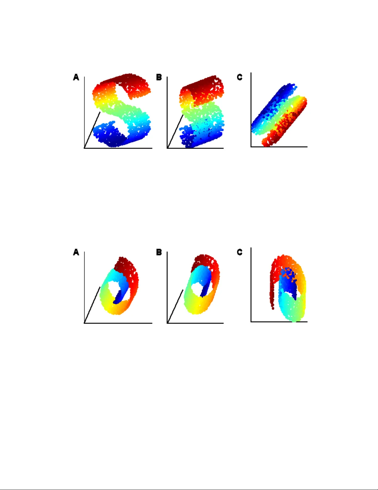
LLE with lo w-dimensional neigh b orho o d represen tation Y air Goldb erg y air go@mail.huji.ac.il Dep artment of Statistics The Hebr ew University, 91905 Jerusalem, Isr ael Y a’aco v Rito v y aa cov.rito v@huji.ac.il Dep artment of Statistics The Hebr ew University, 91905 Jerusalem, Isr ael Editor: ?? Abstract The lo cal linear embedding algorithm (LLE) is a non-linear dimension-reducing technique, widely used due to its computational simplicity and intuitiv e approac h. LLE first linearly reconstructs eac h input p oin t from its nearest neigh b ors and then preserv es these neigh b or- ho od relations in the lo w-dimensional em b edding. W e show that the reconstruction w eigh ts computed b y LLE capture the high -dimensional structure of the neigh b orho ods, and not the low -dimensional manifold structure. Consequently , the weigh t vectors are highly sensi- tiv e to noise. Moreov er, this causes LLE to conv erge to a line ar pro jection of the input, as opp osed to its non-line ar embedding goal. T o o vercome b oth of these problems, w e prop ose to compute the weigh t v ectors using a low-dimensional neigh b orhoo d represen tation. W e pro ve theoretically that this straigh tforward and computationally simple modification of LLE reduces LLE’s sensitivit y to noise. This modification also remo ves the need for regular- ization when the n umber of neigh b ors is larger than the dimension of the input. W e presen t n umerical examples demonstrating b oth the p erturbation and linear pro jection problems, and the improv ed outputs using the low-dimensional neighborho o d representation. Keyw ords: Lo cally Linear Em b edding (LLE), dimension reduction , manifold learning, 1. Introduction The lo cal linear em b edding algorithm (LLE) (Row eis and Saul, 2000) b elongs to a class of recen tly dev elop ed, non-linear dimension-reducing algorithms that include Isomap (T enen- baum et al., 2000), Laplacian Eigenmap (Belkin and Niyogi, 2003), Hessian Eigenmap (Donoho and Grimes, 2004), L TSA (Zhang and Zha, 2004), and MVU (W einberger and Saul, 2006). This group of algorithms assumes that the data is sitting on, or next to, an embedded manifold of lo w dimension within the original high-dimensional space, and attempts to find an em b edding that maps the input p oin ts to the lo wer-dimensional space. Here a manifold is defined as a top ological space that is lo cally equiv alen t to an Euclidean space. LLE w as found to b e useful in data visualization (Row eis and Saul, 2000; Xu et al., 2008) and in image pro cessing applications, suc h as image denoising (Shi et al., 2005) and human face detection (Chen et al., 2007). It is also applied in differen t fields of science such as chem- 1 istry (L’Heureux et al., 2004), biology (W ang et al., 2005), and astroph ysics (Xu et al., 2006). LLE attempts to recov er the domain structure of the input data set in three steps. First, LLE assigns neigh b ors to eac h input p oin t. Second, for each input p oin t LLE computes w eight v ectors that best linearly reconstruct the input point from its neighbors. Finally , LLE finds a set of low-dimensional output p oin ts that minimize the sum of reconstruction errors, under some normalization constraints. In this pap er we fo cus on the computation of the weigh t vectors in the second step of LLE. W e sho w that LLE’s neigh b orho od description captures the structure of the high - dimensional space, and not that of the low -dimensional domain. W e sho w tw o main con- sequences of this observ ation. First, the w eight v ectors are highly sensitive to noise. This implies that a small p erturbation of the input may yield an en tirely different embedding. Second, w e show that LLE conv erges to a linear pro jection of the high-dimensional input when the n umber of input p oin ts tends to infinit y . Numerical results that demonstrate our claims are pro vided. T o o vercome these problems, we suggest a simple mo dification to the second step of LLE, LLE with low-dimensional neighb orho o d r epr esentation . Our approach is based on finding the b est lo w-dimensional represen tation for the neigh b orhoo d of eac h p oin t, and then computing the weigh ts with resp ect to these lo w-dimensional neigh b orho ods. This prop osed mo dification preserv es LLE’s principle of reconstructing eac h p oint from its neighbors. It is of the same computational complexity as LLE and it remov es the need to use regularization when the n umber of neigh b ors is greater than the input dimension. W e pro v e that the weigh ts computed b y LLE with low-dimensional neigh b orhoo d rep- resen tation are robust against noise. W e also pro ve that when using the mo dified LLE on input points sampled from an isometrically em b edded manifold, the pre-image of the input p oin ts achiev es a low v alue of the ob jectiv e function. Finally , we demonstrate an improv e- men t in the output of LLE when using the low-dimensional neighborho od representation for several n umerical examples. There are other w orks that suggest improv emen ts for LLE. The Efficient LLE (Hadid and Pietik¨ ainen, 2003) and the Robust LLE (Chang and Y eung, 2006) algorithms b oth address the problem of outliers b y preprocessing the input data. Other versions of LLE, including ISOLLE (V arini et al., 2006) and Improv ed LLE (W ang et al., 2006), suggest differen t w ays to compute the neigh b ors of eac h input p oint in the first step of LLE. The Mo dified LLE algorithm (Zhang and W ang, 2007) prop oses to improv e LLE by using m ul- tiple lo cal weigh t vectors in LLE’s second step, th us characterizing the high-dimensional neigh b orho od more accurately . All of these algorithms attempt to characterize the high - dimensional neighborho o ds, and not the low -dimensional neighborho o d structure. Other algorithms can b e considered v arian ts of LLE. Laplacian Eigenmap essen tially computes the weigh t vectors using regularization with a large regularization constan t (see discussion on the relation betw een LLE and Laplacian Eigenmap in Belkin and Niyogi, 2003, Section 5). Hessian Eigenmap (Donoho and Grimes, 2004) characterizes the lo cal input neighborho o ds using the null space of the lo cal Hessian op erator, and minimizes the appropriate function for the embedding. Closely related is the L TSA algorithm (Zhang and Zha, 2004), which characterizes eac h lo cal neighborho o d using its local PCA. These last tw o algorithms attempt to describ e the lo w-dimensional neigh b orhoo d. Ho w ever, these 2 algorithms, like Laplacian Eigenmap, do not use LLE’s intuitiv e approac h of reconstruct- ing eac h p oin t from its neighbors. Our prop osed mo dification provides a low-dimensional neigh b orho od description while preserving LLE’s intuitiv e approach. The pap er is organized as follo ws. The description of LLE is presented in Section 2. The discussion of the second step of LLE appears in Section 3. The suggested mo dification of LLE is presen ted in Section 4. Theoretical results regarding LLE with low-dimensional neigh b orho od representation app ear in Section 5. In Section 6 we present n umerical exam- ples. The pro ofs are presented in the App endix. 2. Description of LLE The input data X = { x 1 , . . . , x N } , x i ∈ R D for LLE is assumed to be sitting on or next to a d -dimensional manifold M . W e refer to X as an N × D matrix, where each row stands for an input p oin t. The goal of LLE is to reco ver the underlying d -dimensional structure of the input data X . LLE attempts to do so in three steps. First, LLE assigns neighbors to each input p oin t x i . This can b e done, for example, b y c ho osing the input point’s K -nearest neighbors based on the Euclidian distances in the high-dimensional space. Denote b y { η j } the neigh b ors of x i . Let the neighborho o d matrix of x i b e denoted by X i , where X i is the K × D matrix with rows η j − x i . Second, LLE computes w eights w ij that b est linearly reconstruct x i from its neigh b ors. These weigh ts minimize the reconstruction error function ϕ i ( w i ) = k x i − X j w ij x j k 2 , (1) where w ij = 0 if x j is not a neighbor of x i , and P j w ij = 1. With some abuse of notation, w e will also refer to w i as a K × 1 v ector, where w e omit the entries of w i for non-neigh b or p oin ts. Using this notation, w e ma y write ϕ i ( w i ) = w 0 i X i X 0 i w i . Finally , given the w eights found abov e, LLE finds a set of lo w-dimensional output points Y = { y 1 , . . . , y N } ∈ R d that minimize the sum of reconstruction errors Φ( Y ) = n X i =1 k y i − X j w ij y j k 2 , (2) under the normalization constraints Y 0 1 = 0 and Y 0 Y = I , where 1 is v ector of ones. These constrain ts force a unique minim um of the function Φ. The function Φ( Y ) can be minimized by finding the d -b ottom non-zero eigen vectors of the sparse matrix ( I − W ) 0 ( I − W ), where W is the matrix of weigh ts. Note that the p -th co ordinate ( p = 1 , . . . , d ), found simultaneously for all output p oin ts y i , is equal to the eigen vector with the p -smallest non-zero eigenv alue. This means that the first p co ordinates of the LLE solution in q dimensions, p < q , are exactly the LLE solution in p dimensions (Ro weis and Saul, 2000; Saul and Ro w eis, 2003). Equiv alen tly , if an LLE output of dimension q exists, then a solution for dimension p , p < q , is merely a linear pro jection of the q -dimensional solution on the first p dimensions. When the n umber of neighbors K is greater than the dimension of the input D , each data p oin t can b e reconstructed p erfectly from its neigh b ors, and the local reconstruction 3 w eights are no longer uniquely defined. In this case, regularization is needed and one needs to minimize ϕ reg i ( w i ) = k x i − X j w ij x j k 2 + δ k w i k 2 . (3) where δ is a small constan t. Saul and Ro weis (2003) suggested δ = ∆ K trace( X i X 0 i ) with ∆  1. Regularization can b e problematic for the following reasons. When the regularization constan t is not small enough, it w as shown by Zhang and W ang (2007) that the correct w eight v ectors cannot b e w ell approximated b y the minimizer of ϕ reg i ( w i ). Moreo v er, when the regularization constan t is relatively high, it pro duces w eight v ectors that tend to wards the uniform v ectors w i = (1 /K , . . . , 1 /K ). Consequen tly , the solution for LLE with large regularization constan t is close to that of Laplacian Eigenmap, and do es not reflect a solution based on reconstruction w eigh t v ectors (see Belkin and Niy ogi, 2003, Section 5). In addition, Lee and V erleysen (2007) demonstrated that the regularization parameter m ust b e tuned carefully , since LLE can yield completely differen t embeddings for different v alues of this parameter. How ev er, in real-world data the dimension of the input is typically greater than the num b er of neighbors. Hence, for real-world data, regularization is usually unnecessary . 3. Preserv ation of high-dimensional neigh b orho o d structure by LLE In this section we focus on the computation of the w eigh t vectors, whic h is performed in the second step of LLE. W e first sho w that LLE characterizes the high -dimensional structure of the neigh b orho od. W e explain how this can lead to the failure of LLE in finding a meaningful embedding of the input. Two additional consequences of preserv ation of the high-dimensional neigh b orho od structure are discussed. First, LLE’s w eigh t vectors are sensitiv e to noise. Second, LLE’s output tends to ward a linear pro jection of the input data when the n umber of input p oints tends to infinity . These claims are demonstrated using n umerical examples. W e b egin by showing that LLE preserv es the high-dimensional neighborho od structure. W e use the example that app ears in Fig 1. The input is a sample from an open ring whic h is a one-dimensional manifold em b edded in R 2 . F or eac h p oint on the ring, w e define its neighborho o d using its 4 nearest neigh b ors. Note that its high -dimensional ( D = 2) neigh b orho od structure is curved, while the low -dimensional structure ( d = 1) is a straigh t line. The tw o-dimensional output of LLE (see Fig. 1) is essentially a reconstruction of the input. In other words, LLE’s weigh t vectors preserv e the curv ed shap e of eac h neighborho o d. The one-dimensional output of the open ring is presen ted in Fig 1C. Recall that the one- dimensional solution is a linear pro jection of the tw o-dimensional solution, as explained in section 2. In the op en-ring example, LLE clearly fails to find an appropriate one-dimensional em b edding, b ecause it preserv es the tw o-dimensional curved neighborho o d structure. W e no w sho w that this is also true for additional examples. The ‘S’ curve input data app ears in Fig 2A. Fig 2B sho ws that the ov erall three- dimensional structure of the ‘S’ curve is preserved in the three-dimensional em bedding. The tw o-dimensional output of LLE app ears in Fig 2C. It can b e seen that LLE do es not succeed in finding a meaningful embedding in this case. Fig 3 presen ts the swissroll, with similar results. 4 Figure 1: The input for LLE is the 16-p oin t op en ring that app ears in (A). The tw o- dimensional output of LLE is giv en in (B). LLE finds and preserves the t wo- dimensional structure of each of the lo cal neighborho o ds. The one-dimensional output of LLE app ears in (C). The computation w as p erformed using 4-nearest- neigh b ors, and regularization constant ∆ = 10 − 9 . W e p erformed LLE, here and in all other examples, using the LLE Matlab co de as it app ears on the LLE w ebsite (Saul and Ro w eis). 1 The code that pro duced the input data for the ‘S’ curve and the swissroll was also taken from the LLE website. W e used the default v alues of 2000-p oin t samples and 12- nearest-neigh bors . F or the regularization constant we used ∆ = 10 − 9 . It should be noted that using a large regularization constan t impro ved the results. How ever, as discussed in Section 2, the w eigh t v ectors pro duced in this wa y do not reflect a solution that is based on reconstruction weigh t v ectors. Instead, the vectors tend to ward the uniform vector. W e now discuss the sensitivity of LLE’s weigh t vectors { w i } to noise. Figure 4 sho ws that an arbitrarily small c hange in the neigh b orho od can cause a large change in the w eigh t v ectors. This result can b e understo o d by noting ho w the v ector w i is obtained. It can b e sho wn (Saul and Ro weis, 2003) that w i equals ( X i X 0 i ) − 1 1 , up to normalization. Sensitivity to noise is therefore exp ected when the condition n umber of X i X 0 i is large (see Golub and Loan, 1983, Section 2). One w ay to solv e this problem is to enforce regularization, with its asso ciated problems (see section 2). In the next section w e suggest a simple alternative solution to the sensitivity of LLE to noise. One more implication of the fact that LLE preserv es the high-dimensional neigh b orhoo d structure is that LLE’s output tends to a linear pro jection of the input data. W u and Hu (2006) prov ed for a finite data set that when the reconstruction errors are exactly zero for eac h of the neighborho o ds, and under some dimensionality constrain t, the output of LLE m ust b e a linear pro jection of the input data. Here, w e present a simple argumen t that 1. The changes in the Matlab function eigs were taken into account. 5 Figure 2: (A) LLE’s input, a 2000-p oin t ‘S’ curve. (B) The three-dimensional output of LLE. It can b e seen that LLE finds the o verall three-dimensional structure of the input. (C) The tw o-dimensional output of LLE. Figure 3: (A) LLE’s input, a 2000-point swissroll. (B) The three-dimensional output of LLE. It can b e seen that LLE finds the o verall three-dimensional structure of the input. (C) The tw o-dimensional output of LLE. explains wh y LLE’s output tends to a linear pro jection when the num b er of input p oin ts tends to infinit y , and show n umerical examples that strengthen this claim. F or simplicity , w e assume that the input data is normalized. 6 Figure 4: The effect of a small p erturbation on the weigh t v ector computed by LLE. All three panels show the same unp erturb ed neighborho o d, consisting of a p oin t and its four nearest-neigh b ors (black p oin ts), all sitting in the t w o-dimensional plane. Eac h panel sho ws a different small p erturbation of the original neighborho o d (gra y points). All p erturbations are in the direction orthogonal to the plane of the original neighborho o d. (A) and (C): Both perturbations are in the same direction. (B) P erturbations are of equal size, in opp osite directions. The unique weigh t v ector for the cen ter p oint is denoted for each case. These three different w eight v ectors v ary widely , ev en though the different p erturbations can be arbitrarily small. Our argumen t is based on tw o claims. First, note that LLE’s output for dimension d is a linear-pro jection of LLE’s output for dimension D (see Section 2). Second, note that b y definition, the LLE output is a set of p oin ts Y that minimizes the sum of reconstruction errors Φ( Y ). F or normalized input X of dimension D , when the n umber of input p oin ts tends to infinity , each p oin t is well reconstructed by its neigh b oring p oin ts. Therefore the reconstruction error ϕ i ( w ) tends to zero for each p oin t x i . This means that the input data X tends to minimize the sum of reconstruction errors Φ( Y ). Hence, the output p oin ts Y of LLE for output of dimension D tend to the input p oints (up to a rotation). The result of these t wo claims is that an y requested solution of dimension d < D tends to a linear pro jection of the D -dimensional solution, i.e., a linear pro jection of the input data. The result that LLE tends to a linear pro jection is of asymptotical nature. Ho wev er, n umerical examples sho w that this phenomenon can occur ev en when the num b er of p oin ts is relatively small. This is indeed the case for the outputs of LLE sho wn in Figs. 1C, 2C, and 3C, for the op en ring, the ‘S’ curv e, and the swissroll, resp ectiv ely . 4. Low-dimensional neigh b orho o d represen tation for LLE In this section w e suggest a simple mo dification of LLE that computes the lo w-dimensional structure of the input p oin ts’ neigh b orhoo ds. Our approach is based on finding the b est represen tation of rank d (in the l 2 sense) for the neigh b orhoo d of eac h p oin t, and then com- 7 puting the w eights with resp ect to these d -dimensional neigh b orhoo ds. In Sections 5 and 6 w e show theoretical results and numerical examples that justify our suggested mo dification. W e b egin b y finding a rank- d representation for each local neighborho o d. Recall that X i is the K × D neighborho od matrix of x i , whose j -th ro w is η j − x i , where η j is the j -th neigh b or of x i . W e assume that the num ber of neighbors K is greater than d , since otherwise x i cannot (in general) be reconstructed b y its neighbors. W e say that X P i is the b est rank- d representation of X i , if X P i minimizes   X i − Y   2 o ver all the K × D matrices Y of rank d . Let U LV 0 b e the SVD of X i , where U and V are orthogonal matrices of size K × K and D × D , respectively , and L is a K × D matrix, where L j j = λ j are the singular v alues of X i for j = min( K, D ), ordered from the largest to the low est, and L ij = 0 for i 6 = j . W e denote U =  U 1 , U 2  ; L =  L 1 , 0 0 , L 2  ; V =  V 1 , V 2  (4) where U 1 = ( u 1 , . . . , u d ) and V 1 = ( v 1 , . . . , v d ) are the first d columns of U and V , resp ec- tiv ely , U 2 and V 2 are the last K − d and D − d columns of U and V resp ectiv ely , and L 1 and L 2 are of dimension d × d and ( K − d ) × ( D − d ), respectively . Then by Corollary 2.3-3 of Golub and Loan (1983), X P i can b e written as U 1 L 1 V 0 1 . W e no w compute the w eigh t v ectors for the d -dimensional neighborho o d X P i . By (1), w e need to find w i that minimize w 0 i X P i X P i 0 w i (see Section 2). The solution for this minimiza- tion problem is not unique, since by the construction all the v ectors spanned b y u d +1 , . . . , u K zero this function. Thus, our candidate for the weigh t vector is the vector in the span of u d +1 , . . . , u K that has the smallest l 2 norm. In other words, w e are lo oking for argmin w i ∈ span { u d +1 ,...,u K } w 0 i 1 =1 k w i k 2 . (5) Note that we implicitly assume that 1 / ∈ span { u 1 , . . . , u d } . This is true whenever the neigh b orho od p oin ts are in gener al p osition , i.e., no d + 1 of them lie in a ( d − 1)-dimensional plane. T o understand this, note that if 1 ∈ span { u 1 , . . . , u d } then ( I − 1 K 11 0 ) X P i = ( I − 1 K 11 0 ) U 1 L 1 V 0 1 is of rank d − 1. Since ( I − 1 K 11 0 ) X P i is the pro jected neigh b orho od after cen tering, w e obtained that the dimension of the cen tered pro jected neighborho o d is of dimension d − 1, and not d as assumed, and therefore the points are not in general p osition. See also Assumption (A2) in Section 5 and the discussion that follows. The following Lemma shows ho w to compute the v ector w i that minimizes (5). Lemma 4.1 Assume that the p oints of X P i ar e in gener al p osition. Then the ve ctor w i that minimizes (5) is given by w i = U 2 U 2 0 1 1 0 U 2 U 2 0 1 . (6) The pro of is based on Lagrange m ultipliers and app ears in App endix A.1. F ollowing Lemma 4.1, we prop ose a simple mo dification for LLE based on computing the reconstruction v ectors using d -dimensional neighborho o d represen tation. 8 Algorithm: LLE with low-dimensional neighborho o d represen tation Input : X , an N × D matrix. Output : Y , an N × d matrix. Pro cedure: 1. F or each point x i find K -nearest-neigh bors and compute the neigh b orho od matrix X i . 2. F or each point x i compute the w eigh t vector w i using the d -dimensional neigh b orhoo d represen tation: • Use the SVD decomp osition to write X i = U LV 0 . • W rite U 2 = ( u d +1 . . . , u K ). • Compute w i = U 2 U 2 0 1 1 0 U 2 U 2 0 1 . 3. Compute the d -dimension embedding b y minimizing Φ( Y ) (see (2)). Note that the difference b et ween this algorithm and LLE is in step (2). W e compute the lo w-dimensional neighborho o d represen tation of eac h neighborho o d and obtain its weigh t v ector, while LLE computes the weigh t vector for the original high-dimensional neighbor- ho ods. One consequence of this approach is that the w eight vectors w i are less sensitive to p erturbation, as shown in Theorem 5.1. Another consequence is that the d -dimensional output is no longer a pro jection of the embedding in dimension q , q > d . This is b ecause the w eight v ectors w i are computed differen tly for differen t v alues of output dimension d . In particular, the input data no longer minimize Φ, and therefore the linear pro jection problem do es not o ccur. F rom a computational p oin t of view, the cost of this mo dification is small. F or eac h p oin t x i , the cost of computing the SVD of the matrix X i is O ( D K 3 ). F or N neigh b orho ods w e ha v e O ( N D K 3 ) which is of the same scale as LLE for this step. Since the o verall computation of LLE is O ( N 2 D ), the ov erhead of the modification has little influence on the running time of the algorithm (see Saul and Row eis, 2003, Section 4). 5. Theoretical results In this section we pro ve t wo theoretical results regarding the computation of LLE using the lo w-dimensional neighborho od representation. W e first sho w that a small p erturbation of the neighborho o d has a small effect on the w eigh t v ector. Then w e sho w that the set of original p oin ts in the lo w-dimensional domain that are the pre-image of the input p oin ts ac hieve a low v alue of the ob jectiv e function Φ. W e start with some definitions. Let Ω ⊂ R d b e a compact set and let f : Ω → R D b e a smo oth conformal mapping. This means that the inner pro ducts on the tangent bundle at eac h point are preserved up to a scalar c that may c hange con tin uously from point to p oin t. 9 Note that the class of isometric em beddings is included in the class of conformal em b eddings. Let M b e the d -dimensional image of Ω in R D . Assume that the input X = { x 1 , . . . , x N } is a sample taken from M . F or each p oin t x i , define the neigh b orhoo d X i and its lo w- dimensional representation X P i as in Section 4. Let X i = U LV 0 and X P i = U 1 L 1 V 1 0 b e the SVDs of the i -th neighborho o d and its pro jection, respectively . Denote the singular v alues of X i b y λ i 1 ≥ . . . ≥ λ i K , where λ i j = 0 if D < j ≤ K . Denote the mean v ector of the pro jected i -th neighborho o d b y µ i = 1 K 1 0 X P i . F or the proofs of the theorems w e require that the local high-dimensional neigh b orhoo ds satisfy the follo wing tw o assumptions. (A1) F or eac h i , λ i d +1  λ i d . More sp ecifically , it is enough to demand λ i d +1 < min n ( λ i d ) 2 , λ i d 72 o . (A2) There is an α < 1 suc h that for all i , 1 K 1 0 U 1 U 1 0 1 < α . The first assumption states that for eac h i , the neighborho o d X i is essentially d -dimensional. The second assumption w as sho wn to b e equiv alent to the requirement that p oin ts in each pro jected neighborho o d are in general p osition (see discussion in Section 3). W e now sho w that this is equiv alent to the requiremen t that the v ariance-co v ariance matrix of the pro- jected neighborho o d is not degenerate. Denote S = 1 K X P i 0 X P i = 1 K V 1 L 2 1 V 1 0 , then 1 K 1 0 U 1 U 1 0 1 = 1 K 1 0 ( U 1 L 1 V 1 0 )( V 1 L − 2 1 V 1 0 ) V 1 L 1 U 1 0 1 = µ 0 S − 1 µ . Note that since S − µµ 0 is p ositiv e definite, so is I − S − 1 / 2 µµ 0 S − 1 / 2 . Since the only eigen v alues of I − S − 1 / 2 µµ 0 S − 1 / 2 are 1 and 1 − µ 0 S − 1 µ , we obtain that µ 0 S − 1 µ < 1. Theorem 5.1 L et E i b e a K × D matrix such that k E i k F = 1 . L et e X i = X i + εE i b e a p er- turb ation of the i -th neighb orho o d. Assume (A1) and (A2) and ε < min  ( λ i d ) 4 72 , ( λ i d ) 2 (1 − α ) 72  and that λ i 1 < 1 . L et w i and ˜ w i b e the weight ve ctors for X i and e X i , r esp e ctively, as define d by (5) . Then   w i − ˜ w i   < 20 ε ( λ i d ) 2 (1 − α ) . See pro of in App endix A.3. Note that the assumption that λ i 1 < 1 can alwa ys b e fulfilled b y rescaling the matrix X i since rescaling the input matrix X has no influence on the v alue of w i . Fig 4 demonstrates why no b ound similar to Theorem 5.1 exists for the weigh ts computed b y LLE. In the example w e see a point on the grid with its 4-nearest neigh b ors, where some noise w as added. While λ 1 ≈ λ 2 ≈ 1 − α ≈ 1, and ε is arbitrary , the distance b et w een eac h pair of v ectors is at least 1 2 . The b ound of Theorem 5.1 states that for ε = 10 − 2 , 10 − 4 and 10 − 6 the upp er b ounds on the distance when using the lo w-dimensional neigh b orho od represen tation are is 20 · 10 − 2 , 20 · 10 − 4 and 20 · 10 − 6 resp ectiv ely . The empirical results sho wn in Fig 5 are even lo wer. F or the second theoretical result we require some additional definitions. 10 Figure 5: The effect of neigh b orho od p erturbation on the w eight v ectors of LLE and of LLE with low-dimensional neigh b orho od representation. The original neighborho o d consists of a p oin t on the tw o-dimensional grid and its 4-nearest neigh b ors, as in Fig. 4. A 4-dimensional noise matrix εE where k E k F = 1 was added to the neigh b orho od for ε = 10 − 2 , 10 − 4 and 10 − 6 , with 1000 rep etitions for eac h v alue of ε . Note that no regularization is needed since K = D . The graphs sho w the distance b et w een the v ector w =  1 4 , 1 4 , 1 4 , 1 4  and the vectors computed b y LLE (in green) and by LLE with lo w-dimensional neigh b orho od representation (in blue). Note the log scale in the y axis. The minimum r adius of curvatur e r 0 = r 0 ( M ) is defined as follows: 1 r 0 = max γ ,t    ¨ γ ( t )    where γ v aries ov er all unit-sp eed geodesics in M and t is in a domain of γ . The minimum br anch sep ar ation s 0 = s 0 ( M ) is defined as the largest positive n umber for whic h   x − ˜ x   < s 0 implies d M ( x, ˜ x ) ≤ π r 0 , where x, ˜ x ∈ M and d M ( x, ˜ x ) is the geodesic distance b et ween x and ˜ x (see Bernstein et al., 2000, for b oth definitions). Define the radius r ( i ) of neighborho o d i to b e r ( i ) = max j ∈{ 1 ,...,K }   η j − x i   where η j is the j -th neigh b or of x i . Finally , define r max to b e the maxim um ov er r ( i ) . W e sa y that the sample is dense with respect to the chosen neighborho o ds if r max < s 0 . Note that this condition depends on the manifold structure, the giv en sample, and the c hoice of neighborho o ds. How ever, for a given compact manifold, if the distribution that pro duces the sample is supp orted throughout the en tire manifold, then this condition is v alid with probabilit y increasing tow ards 1 as the size of the sample is increased and the radius of the neighborho ods is decreased. 11 Theorem 5.2 L et Ω b e a c omp act c onvex set. L et f : Ω → R D b e a smo oth c onformal mapping. L et X b e an N -p oint sample taken fr om f (Ω) , and let Z = f − 1 ( X ) , i.e., z i = f − 1 ( x i ) . Assume that the sample X is dense with r esp e ct to the choic e of neighb orho o ds and that assumptions (A1)and (A2) hold. Then, if the weight ve ctors ar e chosen ac c or ding to (6) , Φ( Z ) N = max i λ i d +1 O  r 2 max  . (7) See pro of in Appendix A.3. The theorem states that the original pre-image data Z has a small v alue of Φ and thus is a reasonable embedding, although not necessarily the minimizer (see Goldb erg et al., 2008). This observ ation is not trivial from t w o reasons. First, it is not known a-priori that { f − 1 ( η j ) } , the pre-image of the neighbors of x i , are also neighbors of z i = f − 1 ( x i ). When short-circuits o ccur, this need not to b e true (see Balasubramanian et al., 2002). Second, the weigh t vectors { w i } characterized the pro jected neighborho od, w hic h is only an appro ximation to the true neighborho o d. Nev ertheless, the theorem shows the Z has a lo w Φ v alue. 6. Numerical results In this section w e present empirical results for LLE and LLE with low-dimensional neigh- b orhoo d representation on some data sets. F or LLE, w e used the Matlab co de as app ears in LLE w ebsite (Saul and Row eis). The co de for LLE with low-dimensional neighborho o d represen tation is based on the LLE co de and differs only in step (2) of the algorithm and is a v ailable in JRhomepage. . W e ran LLE with lo w-dimensional neighborho o d representation on the data sets of the op en ring, the ‘S’-curv e and the swissroll that app ear in Figs 1-3. W e used the same parameters for both LLE and LLE with lo w-dimensional neigh b orhoo d represen tation ( K = 4 for the op en ring and K = 12 for the ‘S’-curve and the swissroll). The results app ear in Fig 6. W e ran b oth LLE and LLE with lo w-dimensional neighborho o d represen tation on 64 b y 64 pixel images of a face, rendered with differen t p oses and lighting directions. The 698 images and their resp ectiv e p oses and lighting directions can be found at the Isomap w ebpage (T enenbaum et al.). The results of LLE, with K = 12, are giv en in Fig. 7. W e also chec k ed for K = 8 , 16; in all cases LLE do es not succeed in retrieving the pose and ligh ting directions. The results for LLE with low-dimensional neigh b orhoo d representation, also with K = 12, appear in Fig 8. The left-right p ose and the lighting directions were disco vered by LLE with lo w-dimensional neigh borho o d represen tation. W e also chec k ed for K = 8 , 16; the results are roughly the same. Ac kno wledgments This researc h w as supp orted in part b y Israeli Science F oundation gran t. Helpful discussions with Alon Zak ai and Jacob Goldb erger are gratefully ackno wledged. 12 Figure 6: The inputs app ear in the left column. The results of LLE app ear in the middle column and the the results of LLE with lo w-dimensional represen tation app ear in right column. App endix A. Pro ofs A.1 Pro of of Lemma 4.1 Pro of W rite w i = P K m = d +1 a m u m = U 2 a . The Lagrangian of the problem can b e written as L ( a, λ ) = 1 2 a 0 U 2 0 U 2 a + λ ( 1 0 U 2 a − 1) . T aking deriv atives with resp ect to b oth a and λ , w e obtain ∂ L ∂ a = U 2 0 U 2 a − λU 2 0 1 = a − λU 2 0 1 , ∂ L ∂ λ = 1 0 U 2 a − 1 . Hence we obtain that a = U 2 0 1 1 0 U 2 U 2 0 1 . 13 Figure 7: The first t w o dimensions out of the three-dimensional output of LLE for the faces database appear in all three panels. (A) is colored according to the right-left p ose, (B) is colored according to the up-down pose, and (C) is colored according to the ligh ting direction. Figure 8: The output of LLE with lo w-dimensional neighborho o d represen tation is colored according to the left-right p ose. LLE with low-dimensional neighborho o d repre- sen tation also succeeds in finding the ligh ting direction. The up-down p ose is not fully recov ered. 14 A.2 Pro of of Theorem 5.1 Pro of The pro of of Theorem 5.1 consists of t w o steps. First, w e find a representation of the v ector ˜ w i , the weigh t v ector of the p erturb ed neighborho o d, see (12). Then we b ound the distance betw een ˜ w i and w i , the w eight v ector of the original neigh b orho od. W e start with some notations. F or ev ery matrix A , let λ j ( A ) b e the j -th singular v alue of A . Note that k A k 2 = λ 1 ( A ). In this notation, we ha ve λ i j = λ j ( X i ). Denote b y T = X i 0 X i and e T = e X 0 i e X i = T + ε ( X i 0 E i + E i 0 X i ) + ε 2 E i 0 E i . Using the decomp osition of (4), we ma y write T = U L 2 U 0 and e T = e U e L 2 e U 0 . Note that λ j ( T ) = λ j ( X i ) 2 . Define U 2 and e U 2 to b e the K × ( K − d ) matrices of the left-singular vectors corresponding to the low est singular v alues, as in (4). Note that by assumption, λ 1 ( E i ) = 1, hence, λ 1 ( X i 0 E i ) ≤ λ i 1 ≤ 1. By Corollary 8.1-3 of Golub and Loan (1983), λ i ( T ) − 3 ε ≤ λ i ( e T ) ≤ λ i ( T ) + 3 ε . (8) Let δ = λ d ( T ) − λ d +1 ( T ) − ε . By Theorem 8.1-7 of Golub and Loan (1983), there is a d × ( K − d ) matrix Q such that k Q k 2 ≤ 6 ε δ and suc h that the columns of b U 2 = ( U 2 + U 1 Q )( I + Q 0 Q ) − 1 / 2 are an orthogonal basis for an in v arian t subspace of e T . W e wan t to sho w that b U 2 and e U 2 spans the same subspaces. T o pro v e this, w e b ound the largest singular v alue of k b U 0 2 e T b U 2 k 2 , and the result follows from (8). First, note that 1 − 6 ε δ < λ j  ( I + Q 0 Q ) − 1 / 2  < 1 + 6 ε δ . (9) Hence,   b U 0 2 e T b U 2   2 =   ( I + Q 0 Q ) − 1 / 2 ( U 2 + U 1 Q ) 0 e T ( U 2 + U 1 Q )( I + Q 0 Q ) − 1 / 2   2 ≤  1 + 6 ελ i 1 δ  2    U 0 2 e T U 2   2 + 2   U 0 2 e T U 1 Q   2 +   Q 0 U 0 1 e T U 1 Q   2  ≤  1 + 6 ε δ  2 ( λ d +1 ( T ) + 3 ε ) + (6 ε ) 2 δ +  6 ε δ  2 (1 + 3 ε ) ! . (10) W e now obtain some b ounds on the size of ε . By assumption w e ha ve ε < ( λ i d ) 4 72 . Since assumption (A1) holds, we may assume that λ d +1 ( T ) < λ d ( T ) 72 . Recall that δ = λ d ( T ) − λ d +1 ( T ) − ε and that ( λ i d ) 2 = λ d ( T ). Isolating ε we obtain that ε < λ d ( T ) δ 60 . Similarly , w e can show that ε < δ 2 60 . W e also hav e ε < λ d ( T ) 72 , since by assumption λ d ( T ) < 1, and similarly , ε < δ 60 . Summarizing, we ha v e ε < min  δ 60 , λ d ( T ) 72 , λ d ( T ) δ 60 , δ 2 60  (11) W e are no w ready to b ound the expression in (10). W e ha ve that (1 + 6 ε δ ) < 11 10 since ε < δ 60 ; λ d +1 ( T ) < λ d ( T ) 72 b y assumption; 3 ε < λ d ( T ) 24 since ε < λ d ( T ) 72 ; (6 ε ) 2 δ < λ d ( T ) 120 since 15 ε < δ 60 and also ε < λ d ( T ) 72 ; (6 ε ) 2 δ 2 < λ d ( T ) 100 since ε < λ d ( T ) δ 60 and ε < δ 60 ; 118 ε 3 δ 2 < λ d ( T ) 1000 since ε < δ 60 and ε < λ d ( T ) 72 . Com bining all these b ounds, we obtain   b U 0 2 e T b U 2   2 < λ d ( T ) 10 < λ d ( T ) − 3 ε . Hence, by (8) w e hav e   b U 0 2 e T b U 2   2 < λ d ( e T ). Since b U 2 spans a subspace of K − d dimension, it must span the subspace with the K − d v ectors with lo west singular v alues of e T . In other w ords, b U 2 spans the same subspace as e U 2 or equiv alently b U 2 b U 0 2 = e U 2 e U 0 2 . Summarizing, w e obtained that ˜ w i = b U 2 b U 0 2 1 1 0 b U 2 b U 0 2 1 . (12) W e are now ready to b ound the difference b et ween w i and ˜ w i .   w i − ˜ w i   2 =      U 2 U 2 0 1 1 0 U 2 U 2 0 1 − e U 2 b U 0 2 1 1 0 b U 2 b U 0 2 1      2 = 1 1 0 U 2 U 2 0 1 − 2 1 0 U 2 U 2 0 b U 2 b U 0 2 1 1 0 U 2 U 2 0 11 0 b U 2 b U 0 2 1 + 1 1 0 b U 2 b U 0 2 1 = 1 0 ( U 2 − b U 2 )( U 2 − b U 2 ) 0 1 1 0 U 2 U 2 0 11 0 b U 2 b U 0 2 1 W e use Assumption (A2) to obtain a b ound on 1 0 U 2 U 2 0 1 . Denote the pro jection of the normalized vector 1 √ K 1 on the basis { u j } by p j = 1 √ K 1 0 u i . W e hav e that k µ i k 2 = 1 K   1 √ K 1 0 U 1 L 1   2 = 1 K d X j =1  p j λ i j  2 . By assumption (A2), k µ i k 2 < α K  λ i d  2 . Hence P d j =1 p 2 j < α . Since P K j =1 p 2 j = 1, w e ha ve that K X j = d +1 p 2 j = 1 K 1 0 U 2 U 2 0 1 > 1 − α . (13) Similarly , w e obtain a b ound on 1 0 b U 2 b U 0 2 1 . 1 0 b U 2 b U 0 2 1 ≥   ( I + Q 0 Q ) − 1 / 2 U 0 2 1   2 − 2   1 0 U 1 Q ( I + Q 0 Q ) − 1 U 0 2 1   ≥ (1 − 6 ε δ ) 2 K (1 − α ) − 2 K 6 ε δ (1 + 6 ε δ ) 2 (1 − α ) 1 / 2 ≥ 9 K (1 − α ) 10 − 12 K ε δ  11 10  2 (1 − α ) 1 / 2 , where we used ε < δ 60 . Since b y assumption ε < λ d ( T ) √ (1 − α ) 72 , and using the facts that λ d +1 ( T ) < λ d ( T ) 72 and ε < λ d ( T ) 72 , we obtain that ε < δ √ (1 − α ) 60 . Hence, 1 0 b U 2 b U 0 2 1 ≥ K (1 − α ) 2 . 16 Finally , w e obtain a b ound on 1 0 ( U 2 − b U 2 )( U 2 − b U 2 ) 0 1 .   U 2 − b U 2   2 =   U 2 ( I − ( I + Q 0 Q ) − 1 / 2 ) + U 1 Q ( I + Q 0 Q ) − 1 / 2   2 ≤   U 2   2   I − ( I + Q 0 Q ) − 1 / 2   2 +   U 1   2   Q   2   ( I + Q 0 Q ) − 1 / 2   2 ≤ 6 ε δ + 6 ε δ (1 + 6 ε δ ) = 6 ε δ (2 + 6 ε δ ) where the last inequalit y follo ws from (9), the fact that for an y eigenv ector v of ( I + Q 0 Q ) − 1 / 2 with eigenv alue λ v , v is also eigenv ector of I − ( I + Q 0 Q ) − 1 / 2 with eigenv alue 1 − λ v , and the fact that k A k 2 = 1 for every matrix A with orthonormal columns (see Golub and Loan, 1983). Consequen tly ,   ( U 2 − b U 2 ) 0 1   2 ≤ K 6 ε δ  2 + 6 ε δ  < 13 K ε δ where we used ε < δ 60 . Com bining these results, we hav e   w i − ˜ w i   < (13 K ε ) /δ ( K (1 − α )) / √ 2 < 20 ε λ d ( T )(1 − α ) , where we used 21 20 λ d ( T ) > 1 δ . A.3 Pro of of Theorem 5.2 Pro of Since Φ( Z ) = P N i =1   P j w ij ( z j − z i )   2 , we b ound each summand separately in order to obtain a global b ound. Let the induced neigh b ors of z i = f − 1 ( x i ) b e defined by ( τ 1 , . . . , τ K ) = ( f − 1 ( η 1 ) , . . . , f − 1 ( η K )). Note that a-priori, it is not clear that τ j are neigh b ors of z i . Let J b e the Jacobian of the function f at z i . Since f is a conformal mapping, J 0 J = c ( z i ) I , for some p ositiv e c : Ω → R . Using first order appro ximation w e ha ve that η j − x i = J ( τ j − z i ) + O    τ j − z i   2  . Hence, for w i w e ha ve, K X j =1 w ij ( τ j − z i ) = K X j =1 w ij J 0 ( η j − x i ) + O  max j   τ j − z i   2  . Th us w e hav e   K X j =1 w ij ( τ j − z i )   2 =   K X j =1 w ij J 0 ( η j − x i )   2 +   K X j =1 w ij J 0 ( η j − x i )   O  max j   τ j − z i   2  . (14) W e b ound   P K j =1 w ij J 0 ( η j − x i )   for the v ector w i that minimizes (5). Note that b y (4), P K j =1 w ij J 0 ( η j − x i ) = w 0 i X P i J + w 0 i U 2 L 2 V 0 2 J . Ho wev er, by construction w 0 i X P i = 0. Hence   K X j =1 w ij J 0 ( η j − x i )   =   w 0 i U 2 L 2 V 0 2 J   ≤   w i     U 2 L 2 V 2 0 J   2 ≤   w i   λ i d +1 p c ( z i ) , 17 where w e used the facts that k Ax k 2 ≤ k A k 2 k x k 2 for a any matrix A , and that k A k 2 = 1 for a matrix A with orthonormal columns (see Section 2 of Golub and Loan, 1983, for b oth). Substituting in (14), we obtain   K X j =1 w ij ( τ j − z i )   2 ≤   w i   2 ( λ i d +1 ) 2 c ( z i ) +   w i   λ i d +1 O  max j   τ j − z i   2  . Since assumption (A2) hold, it follo ws from (13) that   w i   2 = 1 1 0 U 2 U 2 0 1 < 1 K (1 − α ) . As f is an conformal mapping, w e ha ve c min   τ j − z i   ≤ d M ( η j , x i ), where d M is the geo desic metric and c min > 0 is the minimum of the scale function c ( z ) that measures the scaling c hange of f at z . The minim um c min is attained as Ω is compact. The last inequality holds true since the geo desic distance d M ( η j , x i ) is equal to the integral o v er c ( z ) for some path b et ween τ j and z i . The sample is assumed to b e dense, hence   τ j − x i   < s 0 , where s 0 is the minimum br anch sep ar ation (see Section 5). Using Bernstein et al. (2000), Lemma 3, we conclude that   τ j − z i   ≤ 1 c min d M ( η j , x i ) < π 2 c min   η j − x i   . Since assumption (A1) holds, and r ( i ) 2 = max j k η j − x i k 2 ≥ 1 K K X j =1 k η j − x i k 2 = k X i k 2 F = 1 K K X j =1 ( λ i j ) 2 ≥ d K ( λ i d ) 2 , w e ha ve λ d +1  r ( i ). Hence   P K j =1 w ij ( τ j − z i )   2 = λ i d +1 O  r ( i ) 2  . References M. Balasubramanian, E. L. Sc h wartz, J. B. T enenbaum, V. de Silv a, and J. C. Langford. The isomap algorithm and top ological stability . Scienc e , 295(5552):7, 2002. M. Belkin and P . Niyogi. Laplacian Eigenmaps for Dimensionalit y Reduction and Data Represen tation. Neur al Comp. , 15(6):1373–1396, 2003. M. Bernstein, V. de Silv a, J. C. Langford, and J. B. T enenbaum. Graph approximations to geo desics on em b edded manifolds. T ec hnical rep ort, Stanford Universit y , Stanford, Av ailable at http://isomap.stanford.edu , 2000. H. Chang and D. Y. Y eung. Robust lo cally linear em b edding. Pattern R e c o gnition , 39(6): 1053–1065, 2006. J. Chen, R. W ang, S. Y an, S. Shan, X. Chen, and W. Gao. Enhancing h uman face detection b y resampling examples through manifolds. Systems, Man and Cyb ernetics, Part A, IEEE T r ansactions on , 37(6):1017–1028, 2007. D.L. Donoho and C. Grimes. Hessian eigenmaps: Lo cally linear em b edding tec hniques for high-dimensional data. Pr o c. Natl. A c ad. Sci. U.S.A. , 100(10):5591–5596, 2004. 18 Y. Goldb erg, A. Zak ai, D. Kushnir, and Y. Ritov. Manifold learning: The price of normal- ization. T o app ear in JMLR, 2008. G. H. Golub and C. F. V an Loan. Matrix Computations . Johns Hopkins Univ ersity Press, Baltimore, Maryland, 1983. A. Hadid and M. Pietik¨ ainen. Efficient lo cally linear embeddings of imp erfect manifolds. pages 188–201. 2003. J. A. Lee and M. V erleysen. Nonline ar Dimensionality R e duction . Springer, 2007. P . J. L’Heureux, J. Carreau, Y. Bengio, O. Delalleau, and S. Y. Y ue. Lo cally linear em- b edding for dimensionality reduction in qsar. J. Comput. Aide d Mol. Des. , 18:475–482, 2004. S. T. Row eis and L. K. Saul. Nonlinear dimensionalit y reduction by lo cally linear embedding. Scienc e , 290(5500):2323–2326, 2000. L. K. Saul and S. T. Row eis. L o cally L inear E m b edding ( LLE ) homepage. http://www. cs.toronto.edu/ ~ roweis/lle/ . L. K. Saul and S. T. Ro w eis. Think globally , fit locally: unsup ervised learning of low dimensional manifolds. J. Mach. L e arn. R es. , 4:119–155, 2003. ISSN 1533-7928. R. Shi, I. F. Shen, and W. Chen. Image denoising through lo cally linear em b edding. In CGIV ’05: Pr o c e e dings of the International Confer enc e on Computer Gr aphics, Imaging and Visualization , pages 147–152. IEEE Computer So ciet y , 2005. J. B. T enenbaum, V. de Silv a, and J. C. Langford. Isomap homepage. http://isomap. stanford.edu/ . J. B. T enenbaum, V. de Silv a, and J. C. Langford. A global geometric framew ork for nonlinear dimensionality reduction. Scienc e , 290(5500):2319–2323, 2000. C. V arini, A. Degenhard, and T. W. Nattkemper. Isolle: Lle with geo desic distance. Neu- r o c omputing , 69(13-15):1768–1771, 2006. H. W ang, J. Zheng, Z. Y ao, and L. Li. Improv ed lo cally linear embedding through new distance computing. pages 1326–1333. 2006. M. W ang, H. Y ang, Z. H. Xu, and K. C. Chou. Slle for predicting membrane protein t yp es. J. The or. Biol. , 232(1):7–15, 2005. K. Q. W einberger and L. K. Saul. Unsup ervised learning of image manifolds b y semidefinite programming. International Journal of Computer Vision , 70(1):77–90, 2006. F. C. W u and Z. Y. Hu. The LLE and a linear mapping. Pattern R e c o gnition , 39(9): 1799–1804, 2006. W. Xu, X. Lifang, Y. Dan, and H. Zhiyan. Sp eech visualization based on lo cally linear em b edding (lle) for the hearing impaired. In BMEI (2) , pages 502–505, 2008. 19 X. Xu, F. C. W u, Z. Y. Hu, and A. L. Luo. A no vel metho d for the determination of redshifts of normal galaxies b y non-linear dimensionality reduction. Sp e ctr osc opy and Sp e ctr al Analysis , 26(1):182–186, 2006. Z. Zhang and J. W ang. Mlle: Mo dified lo cally linear embedding using multiple weigh ts. In B. Sc h¨ olkopf, J. Platt, and T. Hoffman, editors, A dvanc es in Neur al Information Pr o c essing Systems 19 , pages 1593–1600. MIT Press, Cambridge, MA, 2007. Z. Y. Zhang and H. Y. Zha. Principal manifolds and nonlinear dimensionality reduction via tangent space alignment. SIAM J. Sci. Comp , 26(1):313–338, 2004. 20