Gamma shape mixtures for heavy-tailed distributions

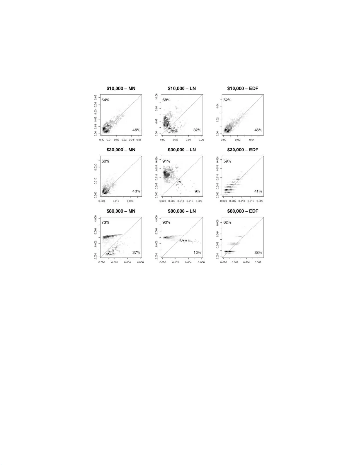
The Annals of Applie d Statistics 2008, V ol. 2, No. 2, 756–776 DOI: 10.1214 /07-A OAS156 c  Institute of Mathematical Statistics , 2 008 GAMMA SHAPE MIXTURES FOR HEA VY-T A ILED DISTRIBUTIONS By Sergio Venturini, Francesc a Dominici an d Gio v anni P armigiani Universit` a Luigi Bo c c oni , Johns Hopkins Scho ol of Public He alth and Johns H opkins University An imp ortant question in health services researc h is the estima- tion of the prop ortion of medical exp enditures that exceed a given threshold. T y pically , medical exp end itures prese nt highly skew ed, heavy tai led distributions, for whic h (a) simple v ariable transforma- tions are insufficient to ac h ieve a tractable lo w-dimensional paramet- ric for m and (b) nonp arametric meth od s are not efficient in esti- mating ex ceedance probab ilities for large thresholds. Motiv ated by this con text, in t h is p ap er w e propose a general Ba yesian a pproac h for the estimation of tail probabilities of h ea v y-tailed d istributions, based on a mixture of gamma distribut ions in which the mixing o c- curs ov er the sh ap e parameter. This family pro vides a fl exible and nov el approach for mo deling heavy-tailed distribu tions, it is compu- tationally efficient, and it only requires to sp ecify a prior distribution for a single parameter. By carrying out simulation stud ies, w e com- pare our approac h with commonly used meth o ds, such as th e log- normal mo del and nonparametric alternatives. W e fo und t h at the mixture-gamma m o del significan tly impro ves predictive p erformance in estimating tail probabilities, compared to t hese alternatives. W e also app lied our metho d to th e Medical Current Benefi ciary S urvey (MCBS), for which we estimate the probabilit y of exceeding a given hospitalization cost for smoking attributab le diseases. W e hav e im- plemented the metho d in th e op en source GSM pac k age, av ailable from the Comprehensive R A rchiv e Netw ork. 1. In tro d uction. In health services r esearc h, there is extensiv e literature on mod els f or pr edicting healt h costs or health services u tilization. These prediction problems are usually complicated b y the nature of the distribu- tions b eing analyzed: high ske wness, h ea viness of th e righ t tail and significan t Received March 2007; revised D ecemb er 2007. Key wor ds and phr ases. Ba yesi an analysis of mix ture distributions, heavy tails, MCBS, medical ex p enditures, tail probability. This is a n electronic r eprint of the original ar ticle published by the Institute of Mathematical Statistics in The Annals of Applie d Statistics , 2008, V ol. 2, No . 2, 7 56–7 76 . This r eprint differs fr om the or iginal in pag ination and typogra phic deta il. 1 2 S. VENTURI NI, F. DOMI N ICI AN D G. P ARMIGIANI fractions of zeros or tok en amoun ts are commonly en coun tered. A t p resen t, there is no agreemen t ab out the b est metho d s to use [see Mullah y and Man- ning ( 2001 ), Kilian et al. ( 2002 ), Bun tin and Zasla vsky ( 2004 ), Barb er and Thompson ( 2004 ), Manning and Mullahy ( 2005 ), Po w ers et al. ( 2005 ), Dod d et al. ( 2004 ); for a r ecen t survey , see Willan and Briggs ( 2006 )]. An imp ortant an d still op en r esearc h question is how to b est predict the prop ortion of (tota l or s ingle-ev en t related) m edical exp enditur es that will exceed a giv en threshold [see, e.g., Briggs and Gray ( 2006 ), Conw ell and Cohen ( 2005 )]. F or example, in s urance companies and go v ernm ental health departments are often in terested in predicting how man y customers or citizens will ask for a r eim b u rsement ab o ve a certain threshold. Similarly , financial institutions are often in terested in estimating the p r obabilit y of the p oten tial loss that could tak e place in the next day , w eek or mon th. In all these situations the parameter of interest is a tail probability of a h ighly sk ewed distrib ution. Thus, it is imp ortant to d evelo p metho ds th at do not simply smo oth the distribu tion of the data, b ut that are able to p erform w ell fr om a pr edictiv e p oin t of view. The wo r k pr esen ted in this article is motiv ated by an an alysis of medical exp enditur es from the Medicare Beneficiaries Su rv ey (MCBS). W e are in- terested in mo d eling the distribution of medical costs paid by the Medicare program for treating s moking attribu table diseases, sp ecifically lung cancer (LC) and coronary h eart disease (CHD). W e need to estimate the p robabil- it y that the h ospitalizatio n cost for a smoking attributable disease exceeds a certain v alue. MCBS is a con tinuous, multipurp ose surv ey of a U.S. nationally r epre- sen tativ e samp le of Medicare b eneficiaries (people aged 65 or older, some p eople under age 65 with disabilities and p eople w ith p ermanent kidney failure requiring dialysis or a kidney transplant). Th e cen tral goal of MCBS is to determine exp enditures and sources of pa ym ent for all services used by Medicare b eneficiaries. The data s et includes medical exp end itures for LC or CHD as p rimary diagnosis for 26,834 hospitalizatio n s of 9,782 individuals for th e p erio d 1999–2 002. F or our analyses, we extract med ical exp end itures on the first hospitalizatio n for 7,615 individuals o v er th e same p erio d . A t ypical assumption in h ealth services researc h is that medical costs are log-normally distributed [Zhou, Gao and Hui ( 1997 ), T u and Zh ou ( 1999 ), Zhou et al. ( 2001 ), Briggs et al. ( 2005 )]. In our case, as well as many others, this assu mption is not app ropriate, since the d istribution of log-transformed exp enditur es is still far fr om b eing symm etric. F or this r eason, new meth- o ds ha v e b een recentl y prop osed for estimating the cost mean difference b et w een t wo groups [Johnson et al. ( 2003 ), Dominici et al. ( 2005 ), Dominici and Z eger ( 2005 )]. How ev er, few m etho ds hav e b een ev aluated for mo deling the entire distribu tion and for pr ediction. GAMMA SH APE MIXTURES 3 The p resence of f ew large observ ations is c haracteristic of skew ed, heavy- tailed d istr ibutions. It is w ell known that these observ ations can influ en ce the results of statistical analyses. T he remed ies prop osed in the health researc h literature are either to transform the d ata [see Duan ( 1983 ), Mullah y ( 1998 ), Manning ( 1998 ), Mullah y an d Mannin g ( 200 1 )] or to use robust metho ds [see Conigliani and T ancredi ( 2005 ), Can toni and Ron chetti ( 1998 )]. Ho w ever, the com b in ation of a transformation with a parametric form ma y still not b e sufficien tly flexible to accommodate large v alues, and also r etains the un - desirable p rop erty of b orro wing information from the left tail to fit the righ t tail. On the other hand , robust m etho ds may discoun t extreme outliers, even though those ma y b e critical in helping d ecision mak ers ev aluate th e change of in cu rring in a very large cost. W e sough t a more reasonable trade-off b y mo d eling the medical cost s distribution using mixture, a direction that has not b een explored in health s ervices researc h as far as w e kn o w. Mix- ture models are parametric mod els whic h are flexible enough to r epresent a large sp ectrum of differen t phenomena. T he mixtu re mo dels literature is extensiv e [for general o verviews, see Titterington, Smith and Mak o v ( 1985 ), Lindsa y ( 1995 ), McLac hlan and Pee l ( 2000 ); for a comprehensiv e list of ap - plications, see Titterington ( 1997 )]. P articularly relev an t for this pap er is the w ell-deve lop ed parametric Ba ye sian literature on m ixture distr ibutions [see Dieb olt and Rob ert ( 1994 ), Rob ert ( 1996 ), Ro eder and W asserman ( 1 997 ), Marin, Mengersen and Rob ert ( 2005 )]. Motiv ated b y these considerations, w e prop ose a new metho d for density estimation of ve ry skew ed distr ibutions and for predicting the p rop ortion of medical exp enditures that exce ed a giv en threshold. W e mo del the d is- tribution of medical exp enditures by use of a m ixture of gamma densit y functions with unkn own w eigh ts. Using this mo del, w e then estimate the tail probabilit y P ( Y > k ), for differen t v alues of k . Eac h gamma distrib u- tion in the mixture is ind exed by a comp onen t-sp ecific shap e parameter and a s ingle unknown scale parameter θ . This parameterization allo ws to create a con v en ien t and fl exible mo del charac terized b y a single p arameter for all the gamma comp onent s, plus the ordinary set of mixture weig h ts. Moreo v er, our parameterizatio n ov ercomes the s o-called “lab el-switc h ing” iden tifi ab ility problem that affects mixture mo d el estimation b y automati- cally providing an ord ering of the mixture comp onen ts. F or a recen t survey on iden tifiabilit y problems in Ba ye sian mixture mo deling, see Jasra, Holmes and Stephens ( 2005 ). The num b er of mixtur e comp onents in our mo del is fixed. W e provide practical advice on h ow to choose it as w ell as the h yp er- parameters of the pr ior on the scale parameter. In a simulatio n s tudy closely mimic king the MC BS data we demonstrate that our metho d has a b etter predictiv e p erformance compared to s tand ard app roac hes. In Section 2 we introd uce the gamma sh ap e m ixture mo del, the estimatio n approac h, and p ro vid e guidance on how to c h o ose p rior hyp er p arameters. In 4 S. VENTURI NI, F. DOMI N ICI AN D G. P ARMIGIANI Section 3 we illustrate the results of the sim u lation stu dy and the d ata anal- ysis. Section 4 con tains a discussion and concludin g remarks. T he Ap p end ix con tains tec h nical details ab out the Gibbs samp ler used. 2. The gamma shap e m ixture mo del. In this sectio n we in tro d uce the gamma shap e mixture (GSM) mo d el. W e b egin b y describin g the lik elihoo d and its main p rop erties. In p articular, we sho w that th e gamma m ixture mo del d o es not suffer f r om iden tifiabilit y problems. W e then p resent the prior str ucture and an app roac h for p osterior calculations. 2.1. Likeliho o d and prior structur e. Let Y b e a p ositiv e ran d om v ariable, for example, nonzero m edical exp enditures. Th e GSM mo del is defined as f ( y | π 1 , . . . , π J , θ ) = J X j =1 π j f j ( y | θ ) , (2.1) where f j ( y | θ ) = θ j Γ( j ) y j − 1 e − θ y , the density f unction of a gamma G a ( j, θ ) ran- dom v ariable. W e assume that the num b er of comp onents J is kno wn and fixed, w h ereas π = ( π 1 , . . . , π J ) is an u nknown v ector of mixtu re weig h ts. Discussion on ho w to c ho ose J will b e pro vided later. In what follo ws, w e denote ( 2.1 ) as G S M ( π , θ | J ). The GSM mo del h as tw o u seful p rop erties: 1. 1 θ is a s cale parameter [Lehmann and Casella ( 1998 )] for the w hole mo del, since f ( y | π 1 , . . . , π J , θ ) = θ · f ( θ · y | π 1 , . . . , π J , 1) . 2. Its momen ts are conv ex com binations of th e momen ts of the Y j | θ ∼ f j ( y | θ ) mixture comp onent s, so that the m th moment is giv en by E [ Y m | π 1 , . . . , π J , θ ] = J X j =1 π j E [ Y m j | θ ] = J X j =1 π j Q m ℓ =1 ( j + ℓ − 1) θ m . A f urther issue related to mixture mo d eling is lab el switching , that is, in- v ariance to p ermutatio n s of the comp onents’ in dexes [see Jasra, Holmes and Stephens ( 2005 )]. A t yp ical solution is to imp ose an identifiability c onstr aint , usually an ordering of either the comp onents means or the v ariances or the mixture weigh ts [see Aitkin and Rubin ( 1985 )]. A nice feature of the GSM mo del ( 2.1 ) is that it automatically imp oses a constrain t on b oth the means and the v ariances, sin ce 1 θ < 2 θ < · · · < J − 1 θ < J θ and 1 θ 2 < 2 θ 2 < · · · < J − 1 θ 2 < J θ 2 . Therefore, the mo del is alw ays iden tified and lab el switc hing is not a concern. GAMMA SH APE MIXTURES 5 W e assum e th at θ and π are indep endent a priori and w e sp ecify the follo wing conjugate prior distributions: θ ∼ G a ( α, β ) , π = ( π 1 , . . . , π J ) ∼ D J  1 J , . . . , 1 J  . In p ractice, choosing the π prior h yp erp arameters equal to 1 /J tends to pro du ce p osterior distributions where only a small subset of th e J mixture w eights will ha v e high prior probabilit y to b e selected at eac h iteration of the MCMC , as we will see in the application. Giv en a sample y = ( y 1 , . . . , y n ) of i.i.d. observ ations from ( 2.1 ), the lik e- liho o d is given by L ( π , θ | y ) = n Y i =1 J X j =1 π j f j ( y i | θ ) . (2.2) Unfortunately this expr ession is u n treatable b ecause it includes J n differ- en t terms [Marin, Mengersen and Rob ert ( 2005 )]. T o o v ercome this h urd le w e use th e so-called missing data represent ation of the mixture [Demp- ster, Laird and Rubin ( 1977 ), T ann er and W ong ( 1987 ), Dieb olt and Rob ert ( 1990 , 1994 )]. Giv en y = ( y 1 , . . . , y n ) from ( 2.1 ), we can asso ciate to eac h y i an in teger x i b et w een 1 and J that id en tifies the comp onent of the mixture generating observ ation y i . Thus, the v ariable x i tak es v alue j with p rior probabilit y π j , 1 ≤ j ≤ J . The v ector x = ( x 1 , . . . , x n ) of comp onent lab els is the missing dat a part of the sample sin ce it is n ot observed. Figur e 1 illus- trates this for our mo d el, highligh ting that y is conditionally indep endent from the mixture w eight s π , giv en the m iss ing data x . Supp ose the missing data x 1 , . . . , x n w ere a v ailable. Then the m o del could b e written as p ( y 1 , . . . , y n | x 1 , . . . , x n , θ ) = θ P n i =1 x i Q n i =1 Γ( x i ) n Y i =1 y x i − 1 i ! e − θ P n i =1 y i . (2.3) Fig. 1. Dir e cte d acyclic gr aph (DA G) f or the missing data r epr esentation of the G S M ( π , θ | J ) mo del. 6 S. VENTURI NI, F. DOMI N ICI AN D G. P ARMIGIANI Th us, u s ing ( 2.3 ) and the priors, the p osterior distribu tion is p ( π 1 , . . . , π J , θ | y 1 , . . . , y n , x 1 , . . . , x n ) (2.4) ∝ J Y j =1 π (1 /J )+ n j − 1 j ! θ α +( P n i =1 x i ) − 1 e − ( β + P n i =1 y i ) θ , where n j = P n i =1 I ( x i = j ) , j = 1 , . . . , J , and I ( · ) is the indicator fun ction. The main consequence of this conditional decomp osition is that, for a giv en missing data vect or x 1 , . . . , x n , th e conju gacy is pr eserv ed and, therefore, the sim ulation can b e easily p erformed, conditional on the missing data x 1 , . . . , x n . 2.2. Computation of the p osterior distribution. W e implement tw o ap- proac hes for estimat ing the unknown parameters of in terest. In the first approac h we estimate th e p osterior distr ibution of π , x and θ by using a Gibbs sampler (details are rep orted in the App end ix ). T o increase the ef- ficiency , we also prop ose a second estimation approac h where w e in tegrate out the scale parameter θ analytica lly . The adv ant age of this s econd strat- egy is b oth compu tational, since the Mark o v c hain run s in a sm aller sp ace, and theoretical, since generally sim u lated v alues are less auto correlated af- ter partial marginalization [Liu ( 1994 ), MacEac hern ( 1994 ), MacEac h ern, Clyde and Liu ( 1999 )]. After h aving in tegrated out θ , the full conditional distrib u tion of the mixture weigh ts is giv en b y p ( π 1 , . . . , π J | y 1 , . . . , y n , x 1 , . . . , x n ) ∝ J Y j =1 π (1 /J )+ n j − 1 j , that is, the D J ( 1 J + n 1 , . . . , 1 J + n J ) Diric hlet distr ib ution. In addition, the full conditional of the i th m issing lab el is then give n b y p ( x i | y , x ( − i ) , π ) = J X j =1 π j y j − 1 i Γ( j ) ( α + P ( − i ) x r ) j ( β + P n r =1 y r ) j P J k =1 π k y k − 1 i Γ( k ) ( α + P ( − i ) x r ) k ( β + P n r =1 y r ) k I ( x i = j ) , (2.5) where x ( − i ) is the x = ( x 1 , . . . , x n ) ve ctor with the i th elemen t deleted, P ( − i ) x r denotes the sum of all the comp onen t lab els except for th e i th one, and ( n ) k = n ( n + 1) · · · ( n + k − 1) is the Poc h hammer symbol [see Abramo witz and S tegun ( 1972 )]. W e assume that α is an in teger, for compu- tation s p eed, and to a v oid o v erflo w errors. See Section A.1 in the App endix for further details. The in tegration of θ imp lies that the missin g data are no longer ind ep end en t. W e ha ve implemen ted this approac h in an R pac k age called GSM [ V enturini, Dominici and P armigiani ( 20 08 )], also av ailable from the C om- prehensive R Archiv e Netw ork ( www.r-pr o ject.org ). GAMMA SH APE MIXTURES 7 2.3. Choic e of hyp erp ar ameters. Our mo del sp ecification only requ ires the u ser to sp ecify thr ee h yp erparameters: the num b er of comp onen ts J , and the α and β from the conjugate prior on θ . Th ough these can b e c hosen based on prior kn o wledge wh en a v ailable, we also prop ose, and use in our application, an informal E m pirical Ba ye s app roac h w hic h uses su mmary statistics of the d ata, lik e th e maxim um and the su m of th e observ ations, to get r easonable v alues. The mean of a GSM r an d om v ariable with distrib ution ( 2.1 ) is µ = E [ Y | π 1 , . . . , π J , θ ] = J X j =1 π j j θ , (2.6) so the scale p arameter θ can b e expressed as θ = 1 µ J X j =1 π j j , (2.7) that is, a wei gh ted a ve r age of the J shap e parameters divided by the m ean. Also, the exp ected v alue of the fu ll conditional distribution of θ is E [ θ | y , x ] = α + P n i =1 x i β + P n i =1 y i = β β + P n i =1 y i · α β + P n i =1 y i β + P n i =1 y i · P n i =1 x i P n i =1 y i (2.8) = ω · α β + (1 − ω ) · ¯ x ¯ y . Equation ( 2.8 ) ind icates that the p osterior mean of θ is a we igh ted a verag e of α/β , the pr ior mean of θ , and ¯ x/ ¯ y . Wh en b oth α → 0 and β → 0 the p r ior b ecomes improp er. Then, for a given v alue of J , a strateg y for c ho osing α and β is as follo ws: 1. Compu te e θ = J / max( y 1 , . . . , y n ) and c h ec k that 1 / e θ ≤ min( y 1 , . . . , y n ); the idea is that, on a v erage, θ should tak e v alues that allo w the set of gamma d istributions in ( 2.1 ) to completely span the range of observ ed v alues (the last gamma distribu tion sh ould hav e a mean not smaller than the maximum observ ation and the first gamma distribution a mean not greater than the minimum observ ation). e θ is hence a candid ate for the prior m ean α/β . 2. Cho ose a v alue for the weig h t of th e prior inf ormation ω in ( 2.8 ). V alues b et w een 0.2 and 0.5 are usually reasonable c hoices. Fix β to ( ω · P n i =1 y i ) / (1 − ω ). 3. Set α b y r ounding to th e closest integ er the quanti t y e θ · β . T he roun ding is n eeded b ecause of the assump tion used to get ( 2.5 ). 8 S. VENTURI NI, F. DOMI N ICI AN D G. P ARMIGIANI Concerning the c hoice of J , the goo dn ess of fi t of the GSM is the result of th e in terp la y among the grids of m th order moments  Q m ℓ =1 ℓ θ m , Q m ℓ =1 ( ℓ + 1) θ m , . . . , Q m ℓ =1 ( ℓ + J − 2) θ m , Q m ℓ =1 ( ℓ + J − 1) θ m  , and the ordered sequen ce of obs er v ations. These grids sh ould con tain suffi- cien t elemen ts to fit the data, therefore, J sh ould b e calibrated to the sp ecific set of data und er examination. Generally sp eaking, a small v alue of J can create a sev ere limita tion to the mo d el, as the set of d ensities a v ailable in the cla ss b eing mixed ma y not b e sufficient ly ric h w ith element s that ha v e a large mean. On the other h and, a to o large v alue do es not cause serious difficulties as the fi t is often robust when there are seve ral gamma d istribu- tions in the class that can serve as b uilding b lo c ks for a particular mixture comp onent . Ho w ever, large J can ca use numerical problems. Sometimes a transformation of the data (lik e a log or a ro ot) can b e useful to hand le these n um erical issu es. In practice, the c hoice of J m ay require more than one iteration. In sp ection of the predictiv e densit y is a practical diagnostic to identify missp ecification of J . 3. Results. In this sectio n we carry out a sim ulation study to assess the predictiv e p er f ormance of the gamma m ixture mod el in a con trolled situation in which a large test set is a v ailable to serve as the gold stand ard. Our sim ulation r eflects closely the estimation of the right tail of th e medical exp enditur es distribution for smoking attributable diseases (CHD and LC) from the MCBS. W e compare our mo del with other p opular metho d s in health services researc h. The results sh ow that these standard approac hes are less effectiv e in r eal life situations. In addition, w e apply our metho d s to the MCBS data for estimating the risk for p ersons affec ted by sm oking attributable diseases to exceed a giv en medical costs threshold in a single hospitalizatio n. 3.1. Simulation design. F r om the complete MCBS data for the p er io d 1999– 2002, w e extract exp end iture d ata on hospitalizatio ns in whic h the fir s t diagnosis has b een CHD, LC, or b oth, for a total of 7,615 hosp italizat ions. T ables 1 and 2 r ep ort a br ief su mmary of the d ataset. F rom this p opulation, w e drew 500 sub-samp les, the tr aining sets , of size equal to 10% of the original sample. F or eac h dra w , th e remaining 90% constitute the test set . On eac h training set w e estimate the tail probabilit y ˆ p = P ( y ∗ > k | y ) us ing the f ollo wing four app roac hes: EDF Th e empirical pr op ortion of cases exceeding the threshold, or the em- pirical d istribution f unction (EDF), wh ic h provides a straightfo rw ard mo del-free estimate; GAMMA SH APE MIXTURES 9 LN Th e area to the right of k in a log-normal distribution (LN) whose parameters are estimated by maxim um lik eliho o d [see Aitc h ison and Shen ( 1980 ), Zellner ( 1971 )]; this m etho d is commonly used in h ealth economics and pro vid es a b enchmark to assess the gains pro vid ed by our app roac h compared to standard practice; MN Th e area to the right of k in a mixture of norm al distribu tions (MN), estimated assuming an u nkno wn n u mb er of comp onent s using the mclust pac k age in R [see F raley and Raftery ( 2002 , 2006 )]; this is a flexible and commonly used mixture mo del and pr ovides a b enc hm ark to assess th e gains provi ded b y our no vel mixtur e approac h compared to existing mixture approac hes; GSM Th e gamma sh ap e mixtu r e distrib ution (GSM) estimator p rop osed here. F or the GSM, the estimator of the tail pr ob ab ility is defi n ed as P ( y ∗ > k | y ) = Z P ( y ∗ > k | y , θ , π ) f ( θ , π | y ) dθ d π . (3.1) This predictiv e p robabilit y ca n b e estimated from Gibbs sampling realiza- tions by the Rao–Bla ckw ellized estimato r: b P ( y ∗ > k | y ) = 1 M M X m =1 P ( y ∗ > k | θ ( m ) , π ( m ) ) = 1 M M X m =1 J X j =1 π ( m ) j [1 − F j ( k | θ ( m ) )] , where F j ( ·| θ ) is the distrib ution fu nction of a G a ( j, θ ) random v ariable. In this analysis the hyperp arameters for th e GSM are J = 200, α = 12 , 380, β = 3 , 420, and hav e b een c hosen f ollo wing the indications pro vided in Section 2.3 . W e run th e c h ain for 5,000 iterations (1,000 of whic h for b u rn-in). On eac h test set we co mpute the prop ortion p TRUE of exp end itures ex- ceeding k , and use it as the gold standard. W e rep eat the entire analysis for th e follo w ing v alues of the m edical cost threshold k : $10,0 00, $15,00 0, $20,00 0, $30,00 0, $50,000 and $80,0 00 (higher threshold v alues are to o rare to b e worth includin g in the analysis, see T able 2 ). T able 1 Summary of the MCBS dataset: high-or der quantiles of me dic al exp enditur es of first hospitalization f or LC, CHD or b oth Quantile order 75 90 95 97.5 99 99.9 Quantile ($) 8,187.5 15,457. 2 22,485. 6 29,009. 4 40,955. 9 115,060 .6 10 S. VENTURI NI, F. DOMI N ICI AN D G. P ARMIGIANI T able 2 Summary of the MCB S dataset: numb er of hospitalizations with a c ost ab ove a sp e cifie d thr eshold Threshold ($) 10,000 15,000 20,00 0 30,000 50 ,000 80,000 100,00 0 Count 1,468 79 9 503 179 48 24 9 Proportion 0.1928 0.1049 0.0661 0.0235 0.0063 0.0032 0.0012 Fig. 2. Histo gr ams and b oxplots of p ositive Me dic ar e exp enditur es for hospitalizations r e gar ding smoking attributable dise ases (lung c anc er and c or onary he art dise ase) f r om the 1999–20 02 Me di c ar e Curr ent Beneficiaries Survey (for clarity of exp osition, the hi sto gr am of the origi nal exp enditur es has b e en trunc ate d at the top). The d ata are transformed using the cubic r o ot to cont rol numerical o ve r- flo w. The p opulation parameter of interest remains un c h an ged by this trans- formation. Figure 2 rep orts graph ical su mmaries for b oth the u nt ransformed and trans f ormed MCBS data. 3.2. Simulation r esults. Figure 3 summarizes th e results of our s imula- tion, for eac h estimation metho d and eac h k . In p anel (a) we present the relativ e mean s quared err ors, defin ed b y (mse EDF − mse ˆ p ) / mse EDF , wh ere mse ˆ p indicates the mean squared error for the tail probabilit y P ( y ∗ > k | y ) estimated us ing tail probabilit y estimator ˆ p —either LN, MN or GS M. The relativ e mean squ are errors are obtained as the r atios of the av eraged mean GAMMA SH APE MIXTURES 11 Fig. 3. Simulation study. (a) F or differ ent thr eshold values, the p er c ent me an squar e d er- r or r elative to the EDF estimator, that is, [(mse EDF − mse ˆ p ) / mse EDF ] × 100 . (b) F or differ- ent thr eshold values, the p er c ent bias r elative p TR UE , that is, [( E ( ˆ p ) − p TR UE ) /p TR UE ] × 100 . In b oth p anels, cir cles indic ate GSM, diamonds M N and squar es LN. squared errors o v er the 50 0 sub-samples. In panel (b) w e present the rela- tiv e bias ( E ( ˆ p ) − p TRUE ) /p TRUE . Both ratios are multiplied by 100. Negativ e v alues of the relativ e mean squared error imply that the E DF estimator is preferred to ˆ p , while p ositiv e v alues imply that the tail pr obabilit y estimator ˆ p is preferred to the EDF. F or almost all med ical exp enditure thresholds , th e GSM is more efficien t than the estimator based on the empir ical distribu tion function. As exp ected, w e observ e a trend for the relativ e efficiency to increase with th e th r eshold, up to a 27% impro v ement for the h ighest thr eshold. The tail probabilit y estimator based on the log-normal distribu tion p er- forms p o orly . Its m ean squared error r elativ e to the EDF estimator is b elo w − 100% for all the thresholds, with the w orst p erformance corresp onding to hospitalizatio n costs ab o ve $20 , 000. This result is imp ortant pr actically since man y m o dels in health services researc h and health economics are b ased on the assump tion that the medical expen ditures can b e handled u sing log- normal distributions. Also, the estimator based on the m ixture of normal distribu tions p erforms w orse than the EDF, and the p erform an ce wo rsens as the threshold in creases. This fin ding suggests that normal mixtu r es, wh ile flexible, are not completely adequate for heavil y sk ewe d d ata w h en the fo cus of the in ve stigatio n is a small tail probab ility . Figure 3 (b) rep orts th e r elativ e biases, s h o win g that for large k the mix- ture of gamma d istributions is slightl y biased, but less so than the other 12 S. VENTURI NI, F. DOMI N ICI AN D G. P ARMIGIANI Fig. 4. Simulation study: p airwise c omp arison of pr e di ctive p erformanc es. Each p oint r epr esents a sub-sample of the si mulation study. The c o or dinates of e ach p oi nt ar e given by the absolute value of the differ enc e b etwe en the estimate d tail pr ob ability on the tr ai ning and the gold standar d, for the GSM estimator (on the horizontal axes) and for an alternative estimator (on the vertic al axes), as indic ate d on top of e ach plot. Gr aphs on di ffer ent r ows r efer to differ ent me dic al exp enditur e thr esholds. The shading shows the density of the p oints. Also indic ate d ar e the p er c entages of p oints ab ove and b elow the 45 de gr e es line. metho ds. On ce again, the estimator based on the log-normal d istribution is more biased than th e alternativ es, and it almost alw a ys under estimates th e tail probabilit y for the r eference p opulation. The bias increases systemati- cally (in absolute v alue) with the thresh olds, ind icating that the log-normal distribution is not s u fficien tly heavy- tailed to mimic the right tail of these data. Figure 4 allo ws a f urther comparison of the GSM with the other mo dels. In eac h panel we sho w scatterplots of the p erformance of GSM v ers us that of the other estimation metho ds for thr ee th resholds: $10 , 000, $30 , 000 and $80 , 000. A p oin t in these graphs represents a single s u b-sample of the simulatio n study . Wit hin eac h panel, the x-axis is the absolute v alue of the difference GAMMA SH APE MIXTURES 13 Fig. 5. MCBS data analysis. Fit of the GSM mo del to the M C BS me dic al c osts r elate d to smoking attributable dise ases ( n = 7 , 615 hospitalizations). (a) Histo gr am of the cubic r o ot tr ansforme d me dic al c osts to gether with the p osterior me an of the mo del density (solid line). (b) QQ-plot of the est i mate d mo del cumulative pr ob abilities versus the empiric al ones. b et w een the estimat ed tail probability on the training set using the GSM and the gold standard ; the y-axis is compu ted in the same fashion, but for the alternativ e metho d indicated on top of th e panel. Th ese graphs suggest that the GSM p erforms b etter than the other estimation m etho ds f rom a predictiv e p oin t of view, since in ev ery p anel the ma jority of p oints are ab o ve the d iagonal. The h igher the threshold, the more pronounced the result. Moreo v er, eve n if sligh tly biased, most of the times 1 the GSM p erforms b etter than the estimator b ased on the empirical distribution f u nction. 3.3. Analysis of MCBS me dic al c osts data. In this section we present a data analysis of the MCBS dataset. Th e goals of the analysis are to pr ovide estimates of the d en sit y function and of the risk of exceeding a given med- ical cost threshold k in a single hospitalization, with asso ciated probability in terv als. As in the s im u lation study , we restrict th e an alysis to hospitaliza- tions in which th e first d iagnosis has b een for a smoking attribu table disease, CHD or LC. Th e size of the sample is n = 7 , 615. The h yp erparameters for the GSM ha ve b een set to J = 200, α = 124 , 960, β = 34 , 520. T h e data ha v e b een transf orm ed using a cub ic ro ot transform a- tion. W e used 6,000 sampling iterations (1,000 of which as bu r n-in). 1 In Figure 4 only the graphs for some of the av ailable thresholds are sho wn t o a voi d cluttering. 14 S. VENTURI NI, F. DOMI N ICI AN D G. P ARMIGIANI Fig. 6. MCBS data analysis. (a) Distribution of the numb er of mixtur e c om p onents r ep- r esente d in the sample at e ach iter ation of the chain; (b) Posterior me an of the mixtur e weights; (c) Posterior distribution of the mo del me an [se e ( 2.6 )]. The vertic al dashe d line is the sample me an and the solid line i s the kernel density estimator; (d ) Posterior distri- bution of the mo del varianc e. The vertic al dashe d li ne indi c ates the data sampl e varianc e, while the over-imp ose d solid line is the kernel density estimator. The last two p anels ar e useful che cks of whether the key quantities α , β and J have b e en chosen appr opriately. Figure 5 sho w s the fit of the GSM mod el to the MCBS data. Pa n el (a) present s the d ata histogram together with the fitted mod el d ensit y , esti- mated as the av erage o ve r the posterior distribution of the model param- eters π and θ of the mixture densit y ev aluated at a grid of p oin ts. Pa nel (b) rep orts the QQ-plot of the mo del cumulativ e prob ab ilities, ev aluated at the p osterior mean of the mixtur e weig h ts and scale parameter, ve rsus the empirical cum ulativ e probabilities p i = i/ ( n + 1), i = 1 , . . . , n . As it is clear from these graphs, the GSM pro vides a v ery go o d representati on of the data. GAMMA SH APE MIXTURES 15 Fig. 7. MCBS data analysis. Risk to exc e e d a given me dic al c osts thr eshold in a single hospitalization. Each p oint c orr esp onds to the estimate of the pr e dictive p osterior pr ob abil- ity b P ( y ∗ > k | y ) obtaine d wi th the GSM mo del on the MCBS data. Shading r epr esents the 95% cr e dibl e i ntervals. Figure 6 con tains additional resu lts that pro vid e imp ortant insight on h o w the mo d el wo rks. Ev en though J = 200 comp on ents w ere a v ailable, the esti- mation pro cedur e selects, at ev ery iteration, only a small subset, su fficien t to fit the data. P anel (a) sho ws that, a p osteriori, the num b er of selected com- p onents is b et wee n 9 and 20, with m o de at 14. P anel (b) shows the p osterior means of the mixture weigh ts: only few components h a ve a p osterior mean w eight that is substant ially greater than zero. Th is suggests that d espite the a v ailabilit y of J parameters, the p osterior concen trates on a m uc h sm aller subspace. If desired, a simple hard thresholding of the p osterior probabili- ties could p ro du ce a parsimonious representa tion of the mo del based on few mixture comp onen ts. P anels (c) and (d) rep ort the histograms of the m o del mean and v ariance ev aluated at eac h Gibbs sampler iteratio n. The vertica l dashed lines indicate the emp irical sample mean and v ariance. T hese plots are useful to qualitativ ely assess w hether h yp erparameters α , β and J are appropriate for the s amp le at hand. Figure 7 displays the estimates of the tail p robabilit y f or differen t thresh- old v alues. In other w ords, this graph presen ts the “risk” of excee ding a giv en medical costs thresh old in a single hospitalization for p eople affected b y smoking attributable diseases. The 95% credib le inte rv als for eac h thresh- old estimate are also shown. W e also p erformed a set of sensitivit y analyses to p rior hyperp arameters, b y v aryin g ω = β / ( β + P n i =1 y i ) in the range 0.2 –0.5 and found that the results are not significan tly affected. 16 S. VENTURI NI, F. DOMI N ICI AN D G. P ARMIGIANI 4. Discussion. In this p ap er we int ro duced a Ba yesian m ixture mo del for densit y and tail probabilit y estimation of v ery sk ewed distributions. Our approac h is based on a mixture of gamma distributions o ver the sh ap e pa- rameter, or GSM. This family of distrib utions includes comp onents whose means and v ariances increase toget her, offering a con venien t wa y of repr e- sen ting p opulations in wh ic h a small fraction of individu als has an outlying b ehavio r that is difficult to predict. W e also d evelo p a computationally efficie n t algorithm whic h is a mod i- fication of the standard Gibb s sampler used in the Ba y esian literature on mixture d istributions [Rob ert ( 1996 )]. In our approac h w e integrat e out the scale p arameter θ , th us making compu tations more efficien t [Liu ( 1994 )]). Con vergence of our algorithm is, in our exp erience so far, fast and reliable. No tuning parameters are required. O ur implemen tation is av ailable as an R pac k age call ed GSM , whic h can b e obtained from the Comprehensive R Arc hive Net w ork ( www.r-pr o ject.org ). Our appr oac h w as motiv ated by the estimation of the p rop ortion of sub- jects affecte d by s m oking attributable diseases, sp ecifically CHD and L C, that, in a sin gle hospitalization, ha ve a medical b ill exceeding a give n thresh- old. In p articular, we used data from MCBS, a multipurp ose surv ey of a nationally r epresent ativ e sample of Medicare b eneficiaries in th e U.S. How- ev er, in different con texts, one ma y consider taking int o accoun t the actual surve y w eights to get more representa tive estimates of the medical exp en- ditures extreme p ercen tiles. The appr opriate utilization of suc h adju stmen t is still debated in the literature [see , e.g., Gelman ( 2007 ), Lohr ( 1 999 ) and Pfeffermann ( 1993 )]. The large surve y considered in our article allo wed us to p erform a rigorous cross-v alidation exp er im ent in whic h v ery large test sets pro vide a reliable gold standard. In this conte xt w e demonstrated that GS M offer a far more accurate prediction than that pr o vided by the log-normal mo del, commonly utilized in h ealth economics and health s ervices research. W e conclud e that for highly sk ewed data the log-normal mo del is unlike ly to b e appropriate and unc h eck ed use can lead to seriously biased and inefficien t estimate s of tail probabilit y , esp ecially for high thresholds. Th e sim ulation sh o ws that GSM is also comp etitiv e compared to flexible alte rnativ es su c h as norm al mixture mo dels and mo del-free estimators. Additionally , b eing a complete probabilistic s p ecification of the data generation p ro cess, it can b e us ed for an y other inferenti al pu rp ose. Fitting a GSM mo del requires selecting the maxim u m num b er of mixture comp onent s J . A p ossible generalizati on is to incorp orate the mo del in to a rev ersib le jump app roac h, as prop osed b y Ric hard son and Green ( 1997 ), in whic h the num b er of comp onent s is random. This w ou ld come at the cost of a su bstan tial increase in the computing time, length of the r equ ired c h ains, and conv ergence m onitoring efforts. How ev er, b ecause of the limited loss GAMMA SH APE MIXTURES 17 in sp ecifying a large J , the to ol w e describ ed is lik ely to b e v ery useful as currentl y prop osed. In our mo del, J does not h av e to fit the data: it only has to b e large enough to con tain all the necessary comp onen ts to fit th e data. In this sense, c ho osing J is more similar to c ho osing a mo del space than a mo del. Also, not ha ving to implemen t and m on itor an RJ-MCMC make s our app roac h more su itable for off-the-shelf use of th e asso ciated s oftw are. Our pr esen tation considered a relativ ely s im p le con text in w h ic h all su b- jects b elong to the same group and are measured once. The logic of our approac h lend s itself to generali zations to more complex scenarios. First, it ma y b e u seful to mo del the scale parameter as a function of co v ariates of in terest. Th is extension wo uld allo w to get a general and robust regres- sion mo d el for skew ed d ata. Second, in medical cost data, there ma y b e a v ailabilit y of m u ltiple hospitalizations records for some sub jects in the su r- v ey . Including this dep endence in th e mod el would allo w for more precise individual-lev el pr edictions. Fin ally , one ma y need to incorp orate censoring. In cost d ata, censoring can b e p resen t b ecause of caps in reim b ursement [see, e.g., Lipscom b et al. ( 199 8 )]. Also, if cost w as not d efined for a single hospitalizatio n b u t r eferred to an extended p erio d, traditional time-to-ev en t censoring would come in to pla y as w ell. APPENDIX: CO MPUT A TIONAL DET AILS A.1. Gibbs sampler for mixture estimation with θ inte grated out. The p osterior distribu tion of ( π 1 , . . . , π J , θ ), giv en the sample ( y 1 , . . . , y n ), can b e written as p ( π 1 , . . . , π J , θ | y 1 , . . . , y n ) ∝ J Y j =1 π (1 /J ) − 1 j ! θ α − 1 e − β θ n Y i =1 J X j =1 π j θ j Γ( j ) y j − 1 i e − θ y i ! . The standard algorithm to implemen t the p osterior sim ulation is rep orted in the next sub s ection. How ev er, to increase efficiency , in our estimat ion approac h w e in tegrate ou t the sca le parameter θ [Liu ( 1994 ), MacEac hern ( 1994 ), MacEac her n , Clyde and Liu ( 1999 )]. Th en ( 2.3 ) b ecomes p ( y 1 , . . . , y n | x 1 , . . . , x n ) = Z ∞ 0 θ P n i =1 x i Q n i =1 Γ( x i ) n Y i =1 y x i − 1 i ! e − θ P n i =1 y i β α Γ( α ) θ α − 1 e − β θ dθ (A.1) = β α Γ( α ) Q n i =1 y x i − 1 i Q n i =1 Γ( x i ) Z ∞ 0 θ α +( P n i =1 x i ) − 1 e − ( β + P n i =1 y i ) θ dθ = β α Γ( α ) Q n i =1 y x i − 1 i Q n i =1 Γ( x i ) Γ( α + P n i =1 x i ) ( β + P n i =1 y i ) α +( P n i =1 x i ) . 18 S. VENTURI NI, F. DOMI N ICI AN D G. P ARMIGIANI Note that the observed data, conditionally on the n onobserv ed ones, are no longer indep en d en t. The in terp retation of this fact is th at θ w as a parame- ter shared b y all the ( y i , x i ) pairs, i = 1 , . . . , n . R emoving θ has introdu ced dep end ence among the data. The fu ll conditional of the mixture weigh ts is h ence give n b y p ( π 1 , . . . , π J | y 1 , . . . , y n , x 1 , . . . , x n ) ∝ J Y j =1 π (1 /J )+ n j − 1 j , while, to get the full conditional of the missing data, w e decomp ose it in to the in dividual f ull conditionals p ( x i | y 1 , . . . , y n , x 1 , . . . , x i − 1 , x i +1 , . . . , x n , π 1 , . . . , π J ) , i ∈ { 1 , . . . , n } . Note that p ( x i | y , x ( − i ) , π ) = J X j =1 p ( x i , x ( − i ) | y , π ) P J k =1 p ( k , x ( − i ) | y , π ) I ( x i = j ) = J X j =1 p ( y | x i , x ( − i ) ) · p ( x i , x ( − i ) | π ) P J k =1 p ( y | k , x ( − i ) ) · p ( k , x ( − i ) | π ) I ( x i = j ) , for i ∈ { 1 , . . . , n } and where x ( − i ) denotes the x = ( x 1 , . . . , x n ) vec tor with the i th elemen t deleted. The second equalit y follo ws fr om p ( x | y , π ) · p ( y | π ) = p ( y | x , π ) · p ( x | π ) and from the conditional indep en dence of y from π , given the m issing data x . Su b stituting ( A.1 ), we obtain p ( x i | y , x ( − i ) , π ) = J X j =1 π j y j − 1 i Γ( j ) Γ( α + P ( − i ) x r + j ) ( β + P n r =1 y r ) j P J k =1 π k y k − 1 i Γ( k ) Γ( α + P ( − i ) x r + k ) ( β + P n r =1 y r ) k I ( x i = j ) , (A.2) where the P ( − i ) x r denotes th e sum of all the comp onen t lab els apart from the i th one. If one further assumes that α ∈ N , then ( A.2 ) can b e fu r ther simplified to p ( x i | y , x ( − i ) , π ) = J X j =1 π j y j − 1 i Γ( j ) ( α + P ( − i ) x r ) j ( β + P n r =1 y r ) j P J k =1 π k y k − 1 i Γ( k ) ( α + P ( − i ) x r ) k ( β + P n r =1 y r ) k I ( x i = j ) , (A.3) where ( n ) k = n ( n + 1) · · · ( n + k − 1 ) is the P o chhammer symb ol [see Abramo w itz and Stegun ( 1972 )]. W e refer to th e w hole fraction insid e th e leftmost s u m- mation as κ ij . In principle, α could b e an y p ositiv e real n umb er, but con- straining it to b e an in teger allo w s us to simplify large quantit ies f r om the n u merator and denominator of ( A.2 ) and, h ence, to easily preven t o ve rflo w errors d uring the calculations. GAMMA SH APE MIXTURES 19 The steps to implement this sim u lation algorithm are then summarized b elo w : • Simulate π | y , x ∼ D J  1 J + n 1 , . . . , 1 J + n J  , where n j = P n i =1 I ( x i = j ), j = 1 , . . . , J . • Simulate, for ev ery i = 1 , . . . , n , p ( x i | y 1 , . . . , y n , x 1 , . . . , x i − 1 , x i +1 , . . . , x n , π 1 , . . . , π J ) = J X j =1 κ ij I ( x i = j ) , with κ ij as d efined ab o ve , j = 1 , . . . , J . • Up date n j , j = 1 , . . . , J . A.2. Standard Gibbs sampler for mixture estimation. The imp lemen- tation of the standard Gibbs samp lin g is straight forw ard and inv olv es the iterativ e simulatio n from ( 2.4 ), for the parameters of the mo del, and from p ( x 1 , . . . , x n | π 1 , . . . , π J , θ , y 1 , . . . , y n ) , for the missing data. The steps for the algorithm are [see, e.g., Rob ert ( 1996 )]: • Simulate θ | y , x , π ∼ G a α + n X i =1 x i , β + n X i =1 y i ! , π | y , x , θ ∼ D J  1 J + n 1 , . . . , 1 J + n J  , where n j = P n i =1 I ( x i = j ), j = 1 , . . . , J . • Simulate, for ev ery i = 1 , . . . , n , p ( x i | y i , π 1 , . . . , π J , θ ) = J X j =1 π ij I ( x i = j ) , where π ij = π j f j ( y i | θ ) P J k =1 π k f k ( y i | θ ) , j = 1 , . . . , J. • Up date n j , j = 1 , . . . , J . Ac kn o wledgments. W e would like to thank the review ers for their helpful commen ts. 20 S. VENTURI NI, F. DOMI N ICI AN D G. P ARMIGIANI SUPPLEMENT AR Y MA TER I AL Gamma shap e mixture (doi: 10.121 4/08-A OAS156 S UPP ). This pac k age implemen ts a Ba yesia n approac h for estimation of a mixture of gamma dis- tributions in whic h the mixing o ccur s o ver the shap e parameter. T h is family pro v id es a flexible and no v el approac h for mo deling hea vy-tailed distribu- tions, it is compu tationally efficient , and it only requir es to s p ecify a prior distribution for a single parameter. REFERENCES Abramow i tz, M. and Stegun, I. A. E. (1972 ). Handb o ok of Mathematic al F unctions with F ormulas, Gr aphs, and Mathematic al T ables , 9th printing. Dov er, New Y ork. MR0208797 Aitchison, J. and Shen, S . M. (1980). Logistic normal d istributions: S ome p rop erties and u ses. Biometrika 67 261–272. MR0581723 Aitkin, M. and Rubin, D. B . (1985). Estimation and hyp othesis testing in finite mixture mod els. J. R oy. Statist. So c. Ser. B 47 67–75. Barber, J. and Thompson, S. (2004). Multiple regression of cost data: Use of generalised linear mo dels. J. He alth Servic es R ese ar ch and Policy 9 197–204. Briggs, A. and G ra y, A. (2006). The distribution of health care costs an d their statistical analysis for economic eva luation. J. He alth Ec onomics 25 198–21 3. Briggs, A., Nixon, R ., Dixon, S. and Thompson, S. (2005). Parametric mod elling of cost d ata: Some sim ulation evidence. He alth Ec onomi cs 14 421–428 . Buntin, M. B. and Zasla vsky, A. M. ( 2004). T oo muc h ado about t wo-part mo dels and t ransformation? Comparing metho ds of mo deling Medicare exp enditu res. J. He alth Ec onomics 23 525–54 2. Cantoni, E. and Ronchetti, E. (1998). A robust approac h for skew ed and h ea vy-tailed outcomes in th e analysis of health care exp enditu res. J. He alth Servic es R ese ar ch and Policy 3 233–245. Conigliani, C. and T ancredi, A. (2005). Semi-parametric mo d elling for costs of health care t echnologies. Statistics i n Me dicine 24 3171–3184. MR2209050 Conwell, L. J. and Cohen, J. W . (2005). Characteristics of p ersons with high medical exp enditures in the U .S. civilian noninstitut ionalized population, 20 02. T echnical re- p ort. Avai lable at www.meps.a hrq.go v/pap ers/st73/stat73 .p df . Agency for Healthcare Researc h and Quality . Dempster, A. P., Laird, N. M. and Rubin, D. B. (1977). Maximum likelihoo d from incomplete data v ia the EM algorithm. J. R oy. Statist. So c. Ser. B 39 1–38. MR0501537 Diebol t, J. and Rober t, C. P. (1990). Ba yesian estimation of finite mixtu re distribu- tions. I . Theoretical aspects. T echnical rep ort 110, Un iv. Pari s VI, Paris . Diebol t, J. and Rober t, C. P. ( 1994). Estimation of finite mixture distributions through Ba yesian sampling. J. Ro y. Statist. So c. Ser. B 56 363–375. MR1281940 Dodd, S., B assi, A., Bodger, K. and Williamson, P. (2004). A comparison of mul- tiv ariable regression models to analyse cost data. J. Evaluation in Clinic al Pr actic e 9 197–204 . Dominici, F., C ope, L., Naiman, D. Q. and Zeger, S . L. (2005). Smo oth quantile ratio estimation (S QUARE). Biometrika 92 543–557. MR2202645 Dominici, F. and Zeger, S. L. (2005). Smooth q uantile ratio estimation with regression: Estimating medical exp enditures for smoking-attributable diseases. Biostatistics 6 505– 519. GAMMA SH APE MIXTURES 21 Duan, N. (1983). Smearing estimate: A n onparametric retransformation metho d. J. Amer. Statist. Asso c. 78 605–61 0. MR0721207 Fraley, C. and Ra fter y, A. E. (2002). Mo del-based clustering, d iscriminan t analysis and d ensity estimation. J. Amer. Statist. Asso c. 97 611–631. MR1951635 Fraley, C. and Rafter y, A. E. (2006). MCLUST V ersion 3 for R: Normal mixture mod eling and model-b ased clustering. T ec h nical Rep ort 504, D ept. Statistics, U niv. W ashington. Gelman, A . (2007). Struggles with survey we igh ting and regres sion mod eling. Statist. Sci. 22 153–164. Jasra, A . , Holmes, C . C. and Stephen s, D. A. ( 2005). Marko v c h ain Monte Carlo metho d s and th e label switc hing problem in Ba yesian mixture mo deling. Statist. Sci. 20 50–67. MR2182987 Johnson, E., Domin ici, F., Griswol d, M. and Zeger, S. L. (2003). Diseas e cases and their medical costs attribuitable to smoking: An analysis of th e national medical exp enditure su rvey. J. Ec onometrics 112 135–151. MR1963235 Kilian, R., Ma tschinge r, H., Loeffler, W ., R oick, C. and Angerm eyer, M. C. (2002). A comparison of metho ds to handle skew distributed cost v ariables in the anal- ysis of the resource consump tion in schizo phrenia treatment. J. Mental He alth Policy and Ec onomics 5 21–31. Lehmann, E. L. an d Casella, G . (1998). T he ory of Point Estimation , 2nd ed. Sp ringer, New Y ork. MR1639875 Lindsa y, B . G. (1995). Mixtur e M o dels: The ory, Ge ometry and Applic ations . IMS, Hay- w ard, CA. Lipscomb, J., Ancukiewicz, M., P armi giani, G., Hasselblad, V., Samsa, G. and Ma tchar, D. B. (1998). Predicting the cost of illness: A comparison of alternative mod els applied to stroke. Me di c al De cision Making 18 S39–S56. Liu, J. S. (1994). The collapsed Gibbs sampler in Ba yesi an compu tations with applications to a gene regulation problem. J. Amer. Statist. Asso c. 89 958–966. MR1294740 Lohr, S . L. (1999). Sampling: Design and Analysis . Dux b ury Press, P acific Grov e, CA. MacE achern, S . N. (1994). Estimating normal means with a conjugate st y le D iric h let process prior. Comm. Statist.—Simul. Comput. 23 727–741. MR1293996 MacE achern, S. N., Cl yde, M. and Liu, J. S. (1999). Sequ ential imp ortance sampling for nonparametric Ba yes mod els: The next generation. Canad. J. Statist. 27 251–267. MR1704407 Manning, W . G. (1998). The logged dep end ent v ariable, heteroscedasticity , and the re- transformation problem. J. He al th Ec onomics 17 283–295. Manning, W. G. and Mullahy, J. (2001). Estimating log mo dels: T o transform or not to transform? J. He alth Ec onomics 20 461–49 4. Marin, J. M., Menge rsen, K. and Rober t, C . P. (2005). Ba yesian mod elling and inference on mixtures of distributions. I n Handb o ok of Statistics 25 (D. Dey and C. R. Rao, eds.) 459–507 . N orth-Holland, A msterdam. McLachl an, G. and Peel, D. (2000). Fini te Mi xtur e Mo dels . Wiley , New Y ork. MR1789474 Mullahy, J. (1998). Much ado ab out tw o: Reconsidering retransformation and the tw o- part mo del in health econometrics. J. He alth Ec onomi cs 17 247–281. Mullahy, J. and Mann ing, W. G. (2005). Generalized mo deling approac hes to risk adjustment of skew ed outcomes data. J. He alth Ec onomics 24 465–488. Pfeffermann, D. (1993 ). The role of sampling w eights when mod eling survey data. Internat. Statist. R ev. 61 310–337. 22 S. VENTURI NI, F. DOMI N ICI AN D G. P ARMIGIANI Po wers, C. A., Meyer, C. M., Roebuck , M. C. and V az iri, B. (2005). Predictive mo d- eling of total healthcare costs using pharmacy claims data: A comparison of alternative econometric cost mo d eling tec hniques. Me dic al Car e 43 1065–10 72. Richardson, S . and Green, P. J. (1997). On Bay esian analysis of mixtures with an unknown number of comp onents (with discussion). J. R oy. Statist. So c. Ser. B 59 731– 792. MR1483213 Ro ber t, C. P. (1996). Mixtures of distributions: In ference and estimatio n. In Markov Chain Monte Carlo in Pr actic e (W. R. Gilks, S. Ric hardson and D. J. Spiegelhalter, eds.) 441–464. Chapman and Hall/CRC, New Y ork. MR1397974 Ro eder, K. and W asserman, L. (1997). Practical Bay esian den sit y estimatio n u sing mixtures of normals. J. Amer . Statist. Asso c. 92 894–902. MR1482121 T anner, M. A. and Wo ng, W. H. ( 1987). The calculation of p osterior distributions by data augmentation. J. Amer. Statist. Asso c. 82 528–540. MR0898357 Titterington, D. M. (1997). Mixture distributions. In Encyclop e di a of Statistic al Sci- enc es 399–407. Wiley , New Y ork. Titterington, D. M., Smith, A. F. M. and Mako v, U. E. (1985). Statistic al Analysis of Finite Mi xtur e Distributions . Wiley , Chichester. MR0838090 Tu, W. and Zhou, X.-H. (1999). A W ald test comparing medical cost based on log-normal distributions with zero va lued costs. Statistics i n Me dicine 18 2749–2761. Venturini, S., D omi nici, F. and P armi giani, G. (2008). Supplemet to “Gamma shap e mixtures for heavy-tailed d istributions.” DOI: 10.1214/08-A OAS156SUPP . Willan, A. R. and B riggs, A. H. (2006). Statistic al Analysis of C ost-Effe ctiveness Data . Wiley , N ew Y ork. MR2269496 Zellner, A. (1971). Bay esian and n on-Bay esian analysis of th e log-normal distribution and log-normal regression. J. Amer. Statist. Asso c. 66 327–330. MR0301837 Zhou, X.-H., G ao, S. and Hui, S. L. (1997). Metho ds for comparing the means of tw o indep endent log-normal samples. Biometrics 53 1129–1135. Zhou, X. -H . , Li, C ., Gao, S. and Ti erney, W. M. (2001). Metho ds for testing eq u alit y of means of health care costs in a paired design stud y . Statistics in Me dici ne 20 1703– 1720. S. Venturini Dip ar timento di S cienze delle Decisioni Universit ` a Comm erciale Luigi Bocconi Viale Isonzo 25 Milano 201 37 It al y E-mail: sergio.ven turini@unib o cconi.it F. Dominici Dep ar tment of Biost a tistics Johns Hopkins S chool of Public Heal th 615 Nor th Wolfe Street Bal timore, Mar y land 21205 USA G. P arm igiani The Sidney Kimm el Comprehensive Ca n cer Center Johns Hopkins Un iversity 550 Nor th Bro adw a y Bal timore, M ar yland 21205 USA