A study of pre-validation

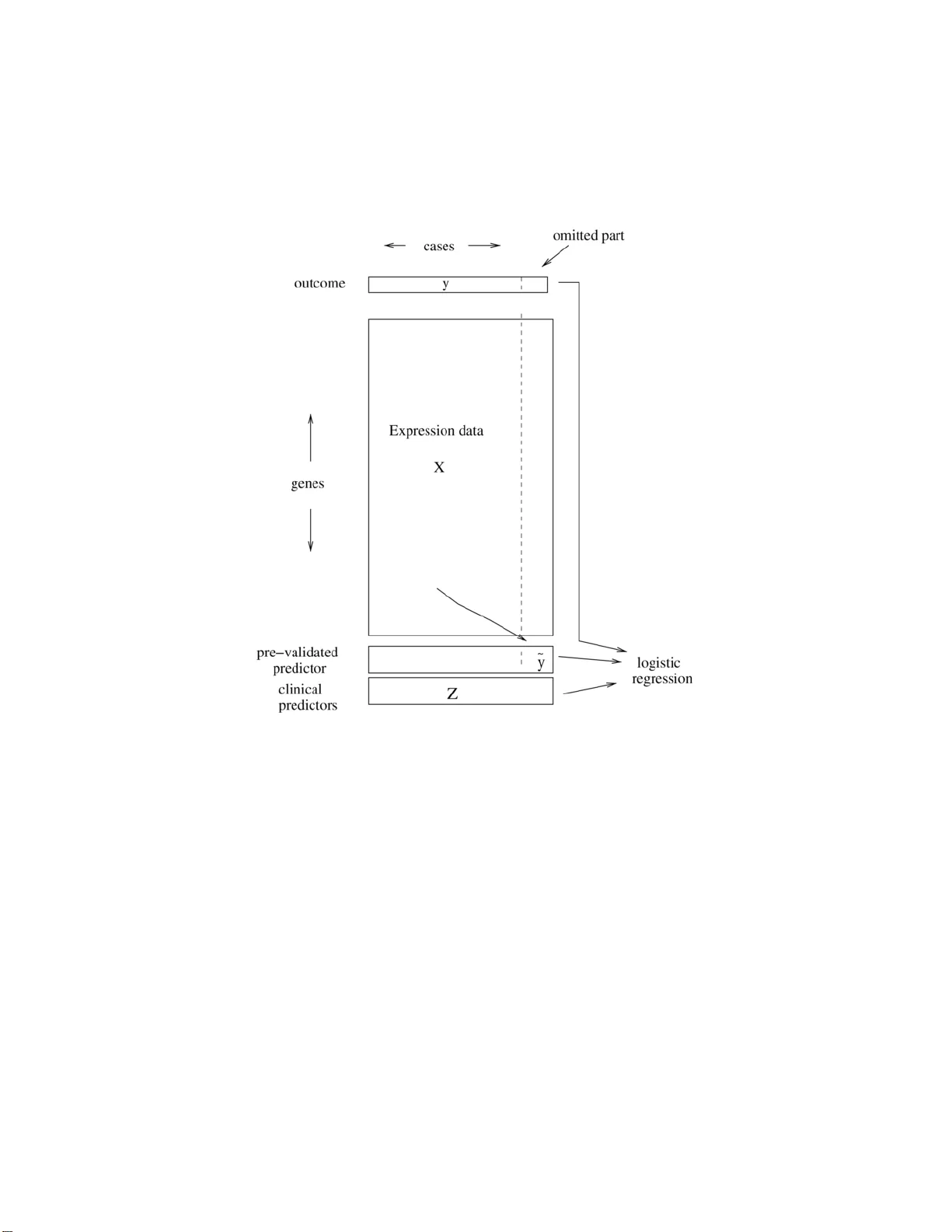
The Annals of Applie d Statistics 2008, V ol. 2, No. 2, 643–664 DOI: 10.1214 /07-A OAS152 c  Institute of Mathematical Statistics , 2 008 A STUD Y OF PRE-V ALIDA TION By Holger H ¨ ofling 1 and R ober t Ti bshirani 2 Stanfor d University Give n a predictor of outcome deriv ed from a high-dimensional dataset, pre-v alidation is a useful technique for comparing it to com- p eting predictors on the same dataset. F or microarra y d ata, it allo ws one to compare a newl y derived predictor for disease outcome to stan- dard clinical predictors on th e same dataset. W e stud y pre-va lidation analytically to determine if the inferences drawn from it are va lid. W e sho w that while pre-v alidation generally w ork s w ell, the straigh tfor- w ard “one degree of freedom” analytical test from pre-v alidation can b e biased and w e prop ose a p ermutation test to remedy th is prob- lem. In sim ulation studies, we show that the p ermutation test has the nominal level and ac h iev es roughly the same p o wer as the analyt ical test. 1. In tro d uction. Supp ose that w e hav e a p rediction rule deriv ed on a high-dimensional dataset. It is often of in terest to compare the n ew predic- tion ru le to comp eting ru les in order to determine if the n ew rule pr ovides an y additional b enefit. F or example, the new prediction rule migh t b e b ased on microarra y expr ession v alues, wh ile th e comp eting predictors are clini- cal, nongenomic measur emen ts. Doing the comparison b et w een the new and comp eting rules on the same dataset (the “re-use” metho d) w ould fav or the new rule as it w as derived on this same dataset. Another approac h wo u ld b e to sp lit the d ata in to separate training and test datasets, build the predictor on the training set and then fi t it along with comp eting pr ed ictors on the test set [see Chang et al. ( 2005 ) for an example]. Ho w ever, with limited d ata, this ma y sev erely r educe the accuracy of the new prediction rule and/or the test set may b e to o s mall to ha ve adequate p o w er for the comparison. Pre-v alidation (PV) [see Tibshirani and Efr on ( 2002 )] offers another ap- proac h to the p r oblem of comparin g a newly deriv ed p rediction ru le to other Received July 2007; revised No vem b er 2007. 1 Supp orted by an Albion W al ter Hewlett Stanford Graduate F ell o wship. 2 Supp orted in part by NSF Grant DMS-99-71405 and NIH Con tract N01-HV-28183. Key wor ds and phr ases. Cross-v alidation, hypothesis testing, p oint estimation, infer- ence, microarra y . This is an electronic repr int of the origina l ar ticle published by the Institute of Mathematical Statistics in The Annals of A pplie d S tatistics , 2008, V ol. 2, No. 2, 643– 664 . This r eprint differs from the or iginal in pagination and t ypo graphic detail. 1 2 H. H ¨ OFLING AND R. TIBSHIRAN I Fig. 1. A schematic of the pr e-validation pr o c ess. The c ases ar e divide d up into (say) 10 e qual-size d gr oups. L e aving out one of the gr oups, a pr e diction rule i s derive d fr om the data of the r emaining 9 gr oups. Thi s pr e diction rule is then applie d to the left out gr oup, gi ving the pr e-validate d pr e dictor ˜ y f or the c ases in the lef t out gr oup. R ep e ating this pr o c ess for every gr oup yields the pr e-validate d pr e dictor ˜ y for al l c ases. Final ly, ˜ y is i nclude d in a lo gistic r e gr ession mo del to gether wi th the clini c al pr e dictors to assess its r elative str ength i n pr e dicting the outc ome. predictors on the same d ataset the new r ule wa s derived on. Pre-v alidation is sim ilar to cross-v alidation, but in stead of directly estimating the predic- tion error, it constructs a “fairer” v ersion of the predictions on the d ata. It uses a pr o cess similar to cross-v a lidation to constru ct predictions for eac h sample, u sing training features for the other observ ations. Thus, the result of pre-v alidation is not an estimate of error (as in cross-v alidation), b ut rather a set of pre-v alidated predictions, one for eac h sample. Th ese p redictions do not ha v e the in heren t bias asso ciated with the re-use metho d . Before going in to more d etails, w e explain ho w p re-v alidatio n w orks on an example (see also Figure 1 ). A STUDY OF PRE- V ALIDA TION 3 W e ha ve microarra y d ata for n p atien ts with b reast cancer. On eac h array , measuremen ts on p genes we re tak en. Also a v ailable are several n onmicroar- ra y based pr edictors, wh ich are commonly u sed in clinical pr actice (e.g., age, tumor size . . . ) to predict if the patien t’s prognosis is p o or or go o d. W e wan t to u se the microarray data in order to p redict the prognosis of a patien t. In PV, the n patien ts are divided in to K -folds. Lea ving out on e fold, a predic- tion rule u s ing the microarra y data for the remaining K − 1 folds is fit (the in tern al mo del). Using this rule, the cancer typ es for the p atients in the left out fold are pr edicted. This wa y , the data of the left out fold is not used in building the r ule and therefore no o ve rfitting o ccurs. Rep eating this pro ce- dure for every fold yields a vecto r of predictions, wh ich we call pr e-validate d . The pr edicted resp ons e for a given patient deriv es from that p atien t’s co v ari- ates through a prediction rule based on indep end en t data. T he p re-v alidated predictor can now b e compared to the other nonmicroarra y-based predic- tions using a logistic regression mo del (the external mo d el). If the coefficien t of the pre-v alidated predictor in the logistic r egression mo d el is significan t, w e conclude that the new microarra y-b ased prediction ru le has an indep en- den t con tribu tion ov er the existing rules. The effect of PV is to r emo ve muc h of the bias that arises from usin g the same data to bu ild the new prediction rule and compare it to the already established ones. Pre-v alidation constructs a fairer version of our p redictor that can b e used on th e same dataset and will act like a predictor app lied to a n ew external dataset. That is, a single pre-v alidated predictor should b ehav e as if its pre- diction rule was derived on an ind ep endent dataset and therefore act just lik e a r egular predictor in a regression mo del. I n particular, s tandard tests for significance of the p r e-v alidate d predictor should w ork. In this article w e will sh o w that pre-v alidation is only partially successful: while the co efficien t estimate for the pre-v alidated p redictor is generally go o d , the standard ana- lytical tests (e.g., t -test) can b e b iased, with a lev el differing from the target lev el. In this p ap er w e prop ose a p ermutation test to solv e this problem. The fo cus of this pap er is th e statisti cal test of s ignifi cance of the new prediction rule. How ev er, as p oin ted out in P ep e et al. ( 2004 ) and W are ( 2006 ), statistical signifi cance d o es not necessarily imply scientific or clini- cal significance. F or example, a predictor that improv es the misclassification rate of a mo del from 55% to 60% migh t b e statistica l significant, b ut th e o ve rall mo del might b e to o inaccurate to use in p ractice. On the other hand, an imp ro ved misclassification rate ma y app ear relev an t, how ev er, it ma y b e due to c hance and statistica lly insignificant. Therefore, it is imp ortant to es- tablish statistical significance as well as practical relev ance. With resp ect to statistica l significance, we can use tests on th e pre-v alidated predictor wh ic h should b e unbiased to giv e an accurate answ er. In order to establish pr ac- tical relev ance measur es like p rediction error, true p ositiv e fraction (TPF) and false p ositiv e fraction (FPF) s h ould b e examined. F or pre-v alidation, 4 H. H ¨ OFLING AND R. TIBSHIRAN I Tibshirani and Efr on ( 2002 ) su ggest a metho d to estimate the impro vemen t in pr ediction error wh en using the newly dev elop ed pr ediction metho d. T h ey sho w th at their metho d works well and remov es muc h of the bias of the re- use method . Their m etho dology can easily b e extended to other measures suc h as TPF and FPF. In th is article w e establish that stand ard analyti- cal tests in regression mo dels for a pr e-v alidat ed pred ictor are biased. This bias m a y lead researc h ers to conclude that a new p rediction ru le is an im- pro vemen t o v er other pred ictors ev en if the new r u le would not h a ve b een significan t with an u n biased test. W e prop ose a p erm utation test to remedy this pr oblem. In S ection 3 PV is app lied to tw o different prediction metho ds on a mi- croarra y dataset of breast cancer patients in order to illustrate how it is used in p ractice. In Section 4 w e w ill establish the b ias of the s tandard test analyticall y in th e simple setting with a linear internal and a linear external mo del. Section 5 outlines th e mo dels that are used in th e simulatio ns, th e amoun t of bias of the analytical test in these mo dels and the p ermutation test. Section 6 presents the r esults of the sim ulations. 2. Pre-v alidatio n. As men tioned ab ov e, deriving a prediction rule and comparing it to other ru les on the same d ataset can lead to a bias in fa vo r of the new rule du e to o v erfi tting. T h is b ias can b e ve ry large and an example of this effect will b e sho w n later in S ection 3 . One wa y to a vo id o verfitting is to use separate training and test datasets as in Ch an g et al. ( 2005 ). Ho we v er, as this is not a very efficien t use of the d ata, w e can extend this approac h in a straigh tforward fashion by cross-v alidation, whic h is just K applications of the training/test dataset approac h. This pro cedure would th en w ork as follo ws: 1. Divide the data in K separate group s. 2. Lea ve out one group and derive the pred iction ru le o v er the r emaining K − 1 groups. 3. Using the n ew prediction rule, predict the outcome for the left out group. 4. Compare th e s trength of the prediction to the already existing predictors for the outcome (e.g., in a linear or logistic regression m o del, dep ending on the t yp e of outcome) only in the left out group . T est if the new pr ed ictor is significant . 5. Rep eat steps 2–4 for every group and a verage the resu lts. Ho we v er, d ep ending on the c hoice of K , there are tradeoffs. If K is small, sa y 2 or 3, the prediction r u le is d er ived on a smaller set of data, thus p ossibly losing accuracy . In situations as with microarra y data, where the num b er of observ ations is usually sm all compared to the amount of a v ailable data, the reduction of p rediction strength due to the lo wer num b er of observ ations can b e su bstan tial. On the other hand, if K is, sa y , 4 or larger, the comparison A STUDY OF PRE- V ALIDA TION 5 to the already existing prediction rules has to b e done on a v ery small n u m b er of obs erv ations. If there are 5 (sa y) other pred ictors and a total of 50 obser v ations, then with K = 5, th e comparison of the new ru le to the 5 old ones w ould ha v e to b e done using only 10 observ ations—it is ve ry unlik ely to find significant effects under these circum s tances. Pre-v alidation (see Figure 1 ) change s this pr o cedure to a void th e for- men tioned problems: 1. Divide the data in K separate group s. 2. Lea ve out one group and derive the pred iction ru le o v er the r emaining K − 1 groups. 3. Using the n ew prediction rule, predict the outcome for the left out group. 4. Rep eat steps 2 and 3 for eac h group. Collect the predictions into a vecto r suc h that one prediction exists for ev er y observ ation in ev ery group (we call this pred ictor “pre-v alidated”). 5. Compare th e s trength of the prediction to the already existing predictors for the outcome (e.g., in a linear or logistic regression mo del, dep end ing on the type of outcome) using all observ ations and the predictor d eriv ed ab o ve. T est if the new pr edictor is significant . The main difference of PV to the CV m etho d ab o v e is th at instead of ev al- uating the p erform ance on ev ery test set separately and then a ve raging the results, P V colle cts a v ector with pre-v alidated pred ictions for ev ery sample. The comparison to comp eting predictors is done afterward. Within PV, an y prediction rule can b e us ed, ev en if the rule itself esti- mates its parameters b y cross-v alidation. An example of this can b e seen in Section 3.2 . With resp ect to the n um b er of folds used in PV, K is u sually c hosen to b e 5 or 10. Lea v e-one-out PV ( K = n ) leads to h igh v ariance in estimates and lo w er v alues w ould decrease the size of the training set too m u c h, as already discussed ab o ve. How ev er, as in PV, the predictions for all observ ations are collected b efore the comparison to the existing predictors, a high v alue of K do es n ot compromise the p ow er of this comparison. When comparing the pre-v alidated p redictor to the existing predictors, usually a linear or logistic regression mo del is fitted (dep end in g on the out- come). The new prediction ru le is judged to m ake a significan t improv emen t o ve r the old rules if the co efficien t of the pre-v alidated predictor is signif- ican tly different fr om 0. As the new r ule p redicts the outcome, significan t v alues for the co efficient would b e p ositiv e. Therefore, instead of a 2-sided test of β P V = 0 vs. β P V 6 = 0 , we can get more p o wer by doing a one-sided test β P V = 0 vs . β P V > 0. F or this, usu ally the standard analytical tests for the mo del (i.e., t -statistic or z-score) are us ed. Ho wev er, as will b e seen in S ections 4 and 6 , this analytical test is biased in man y situations. W e prop ose to use a p erm u tation test in s tead, whic h is explained in detail in Section 5.3 and the p erformance of wh ich is studied in Section 6 . In th e next section we wan t to illustrate ho w PV w orks in pr actice with t wo examples. 6 H. H ¨ OFLING AND R. TIBSHIRAN I 3. Analysis of br east cancer data. Here we ap p ly PV to the d ataset in v an’t V eer et al. ( 2002 ) using the p erm utation test and compare it to the an alytical results. The data consists of microarra y measurements on 4918 genes o v er 78 patient s with b reast cancer. F ort y-four of these b elong to the goo d pr ognosis group (su rviv al of more than 5 years), 34 h a ve a p o or prognosis. Apart from the microarra y data, a num b er of other clinical predictors exist: • T u mor grade (go o d: 1, 2; p o or: 3) • Estrogen receptor (ER) status (go o d: ≤ 10; p o or: > 10) • Progestron receptor (PR) status (go o d: ≤ 10; p o or: > 10) • T u mor size (mm) (go o d: ≤ 20; p o or: > 20) • P atient age (yrs) (go o d: ≤ 40; p o or: > 40) • Angioin v asion (go o d: 0; p oor: 1) In ord er to predict the pr ognosis of a patient, we try tw o m o dels. T he firs t has b een pr op osed by v an’t V eer et al. ( 2002 ), the second is a L 1 p enalized logistic regression m o del. 3.1. V an ’t V e er et al. ( 2002 ) mo del. Based on the microarra y data, v an’t V eer et al. ( 2002 ) constructed a p redictor for the cancer p rognosis in the follo wing wa y : 1. Select the 70 genes that ha ve the highest correlation with the 78 class lab els. 2. Find the centroi d vec tor of the go o d pr ognosis group . 3. Compute the correlation of eac h case w ith the cen troid of the go o d pr og- nosis group. Find the cutoff such that only 3 cases in the p o or prognosis group are misclassified. 4. Classify an y new case as go o d p rognosis if their correlation with the cen troid is larger than th e cutoff. The predictor from this m o del is, lik e the clinical p r edictors, an indicator v ariable. Using a con tinuous resp onse (e.g., pr ob ab ility of b eing in the p o or prognosis group) would b e p ossible, how ev er, w e use ind icator v ariables as it is a b etter matc h to the clinical pr edictors, wh ic h are also indicators. Using other mo dels is also an option whic h we explore with the next ex- ample. How ever, as we only w ant to illustr ate h o w PV works at th is p oint, w e d o not inv estigate if there are any other mo dels that p ossibly giv e b etter p erformance on this dataset. In fact, as w e can s ee in T able 1 , the mo del p ro- p osed by v an’t V eer et al. ( 2002 ) p erforms b etter th an the p enalized logistic regression shown b elo w. An imp ortant part of the p rediction method is the selection of the top 70 genes. In K -fold PV, this selection of the top genes is b eing r ep eated sepa- rately on eac h of the K training sets consisting of ( K − 1 ) folds as the fir st A STUDY OF PRE- V ALIDA TION 7 step of finding the prediction rule. This wa y , the top genes used in the predic- tion are not necessarily the same across the K folds. Zhu, Ambroise and McLac hlan ( 2006 ) ha ve shown that th is reev aluation is imp ortant as selecting the top genes in a pre-pro cessing step and k eeping them fixed across the folds can lead to b iased results. One option to judge the p erformance of th e new pr ed iction rule is to ev al- uate its univ ariate prediction error u sing CV (see T able 1 ). Ho wev er, as we cannot assess this wa y if tw o predictors complement eac h other and therefore impro v e p erformance if used together or not, we instead do a multiv ariate comparison using a logistic regression with th e p re-v alidated predictor as w ell as the other clinical predictors. The resu lt of the m o del fitting with and without using PV can b e found in T able 2 . W e can immediately s ee ho w the significance of the microarra y predictor is reduced wh en 10-fold PV is b eing used and thus the effect of fitting and testing the mo d el on the same data remo ve d. Ho wev er, as PV c ho oses r andom f olds, the results dep en d on the choice of folds. In order to get a clearer p icture of the significance of the microarra y predictor, w e rep eated the 10-fold PV 100 times and a v eraged the resulting p-v alues for the analytical and the p ermutation tests (see T able 3 ). The analytical test declares the microarra y pr edictor to b e s ignifican t, ho w ever, all 3 p ermuta- tion test statistics do not give significan t results, though the difference of the analytical test to the z-score p erm u tation test is quite sm all. A p ossi- ble explanation for these differen t results is the bias of the analytical test, whic h w e in v estigate in Sections 4 and 5.2 . W e also sh o w in Section 6 th at the p er mutation test do es not suffer fr om this p roblem. 3.2. L 1 p enalize d lo gistic r e gr ession. As a second example to illustrate pre-v alidation, w e use a logistic regression mo del to pr edict the prognosis of T able 1 Err or r ates of the new pr e diction rules and the clinic al pr e dictors. The r ates for the new pr e diction rules ar e b ase d on 100 runs of 10 -fold CV Predictor Error rate v an’t V eer et al. ( 2002 ) 0.321 PLR 0.379 Grade 0.333 ER 0.616 Angio 0.333 PR 0.589 Age 0.654 Size 0.320 8 H. H ¨ OFLING AND R. TIBSHIRAN I a patien t based on the microarra y data. P enalized logistic regression (PLR) has b een shown to work wel l for pred icting outcomes using gene expression on other datasets [see Zhu and Hastie ( 2004 )] and here we use an L 1 p enalt y as it implicitly p erforms v ariable selectio n on the genes [see P ark and Hastie ( 2007 ) for an algorithm]. The p enalt y parameter is chosen su c h that exactly 5 , 1 0 , . . . , 45 or 50 genes are included in the mo del and the optimal num b er of genes is determined b y cross-v alidation. The exact pro cedur e f or pre- v alidating this cross-v alidated mo d el is then: 1. Divide the data into K folds. 2. Set aside one fold as the test set, the remaining K − 1 folds are the training set. T able 2 Summary of the c o efficients i n the exte rnal lo gistic mo del with 10 -f ol d PV and without PV using the van ’ t V e er metho d for pr o gnosis pr e di ction. F or e ach c o efficient a test for β = 0 b ase d on the z-sc or e and the devianc e i s given. A l l p-values ar e for two-side d tests exc ept for the z-sc or e p-value of the van ’ t V e er pr e dictor, whi ch i s a one-side d p-value for testing β = 0 versus β > 0 Predictor Metho d Coefficient SD z-score p-v alue ∆ Deviance p-v alue (dev) v an’t V eer No PV 4 . 10 1 . 09 3 . 75 0 . 9 × 10 − 4 25 . 01 5 . 6 × 10 − 7 10-fold PV 1 . 54 0 . 71 2 . 17 0 . 015 5 . 00 0 . 025 Grade No PV − 0 . 70 1 . 00 − 0 . 70 0 . 497 0 . 51 0 . 475 10-fold PV 0 . 56 0 . 75 0 . 75 0 . 452 0 . 56 0 . 453 ER No PV − 0 . 55 1 . 04 − 0 . 53 0 . 596 0 . 28 0 . 596 10-fold PV − 0 . 64 0 . 90 − 0 . 71 0 . 475 0 . 52 0 . 472 Angio No PV 1 . 21 0 . 82 1 . 48 0 . 139 2 . 29 0 . 130 10-fold PV 1 . 35 0 . 65 2 . 08 0 . 038 4 . 57 0 . 033 PR No PV 1 . 21 1 . 06 1 . 15 0 . 251 1 . 39 0 . 238 10-fold PV 0 . 43 0 . 83 0 . 51 0 . 609 0 . 27 0 . 606 Age No PV − 1 . 59 0 . 91 − 1 . 75 0 . 081 3 . 48 0 . 062 10-fold PV − 1 . 46 0 . 69 − 2 . 10 0 . 035 4 . 82 0 . 028 Size No PV 1 . 48 0 . 73 2 . 03 0 . 043 4 . 37 0 . 037 10-fold PV 0 . 84 0 . 60 1 . 40 0 . 161 1 . 96 0 . 162 T able 3 p-values for the van ’ t V e er pr e dictor over 100 runs of the pr e-validation pr o c e dur e. The me an values ar e r ep orte d as wel l as the p er c entage b elow the levels 0 . 01 , 0 . 05 and 0 . 1 Statistic Mean % < 0 . 01 % < 0 . 05 % < 0 . 1 Analytical z-score 0.046 15 66 91 P erm utation with β 0.095 1 27 57 P erm utation with z-score 0.050 17 62 86 P erm utation with deviance 0.139 0 21 42 A STUDY OF PRE- V ALIDA TION 9 T able 4 Summary of the c o efficients i n the exte rnal lo gistic mo del with 10-fold PV and without PV b ase d on the PLR mo del for pr o gnosis pr e diction. F or e ach c o effici ent a test for β = 0 b ase d on the z-sc or e and the devianc e is given. Al l p-values ar e f or two-side d tests exc ept for the z-sc or e p-value of the PLR pr e dictor, which is a one-side d p-value for testing β = 0 versus β > 0 Predictor Metho d Coefficient SD z-s core p-v alue ∆ Deviance p -v alue (dev) PLR No PV 5 . 62 1 . 45 3 . 88 0 . 5 × 10 − 4 39 . 33 3 × 10 − 10 10-fold PV 0 . 72 0 . 65 1 . 10 0 . 135 1 . 23 0 . 268 Grade No PV 0 . 69 0 . 99 0 . 70 0 . 487 0 . 48 0 . 488 10-fold PV 0 . 73 0 . 77 0 . 95 0 . 343 0 . 90 0 . 342 ER No PV 0 . 33 1 . 65 0 . 20 0 . 841 0 . 04 0 . 84 0 10-fold PV − 0 . 58 0 . 87 − 0 . 67 0 . 504 0 . 45 0 . 501 Angio No PV 1 . 05 0 . 91 1 . 15 0 . 250 1 . 34 0 . 24 7 10-fold PV 1 . 38 0 . 64 2 . 16 0 . 031 4 . 94 0 . 026 PR No PV 1 . 41 1 . 60 0 . 88 0 . 380 0 . 85 0 . 35 6 10-fold PV 0 . 21 0 . 81 0 . 26 0 . 795 0 . 07 0 . 794 Age No PV 1 . 05 1 . 31 0 . 80 0 . 425 0 . 70 0 . 40 2 10-fold PV − 1 . 28 0 . 65 − 1 . 97 0 . 049 4 . 06 0 . 044 Size No PV 0 . 75 0 . 89 0 . 85 0 . 395 0 . 71 0 . 40 1 10-fold PV 1 . 13 0 . 58 1 . 93 0 . 053 3 . 83 0 . 050 3. Fit th e p enalized logistic regression mo del on the tr aining set. Use C V on the training set to find the optimal n um b er of genes. 4. Using the mo del with the cross-v alidated num b er of genes, p redict the outcome on the test s et. 5. Rep eat steps 2–4 for all K folds. 6. Compare the pre-v alidated p redictor to the clinical p redictors in a logistic regression mo del. As can b e seen by this example, PV also w orks with prediction metho d s that rely on CV to estimate their parameters. T he r esults using PLR can b e seen in T ables 4 and 5 . As in the example ab ov e, if no PV is b eing u sed, the predictor app ears to b e highly s ignifican t. Ho w ever, using PV, th e analytica l test giv es a on e-sided p-v alue of 0 . 1349, which is not significant . Using the p ermutati on tests instead confirms this result. Ov erall we can see that the metho d p rop osed b y v an’t V eer et al. ( 2002 ) p erforms b etter on this dataset. In the next section w e analytically sho w in a simple case that the analytical test of significance of a pr e-v alidated predictor based on the t -statistic is biased. 4. Analytical results on the b ias of tests for pre-v alidated predictors. An analytical treatmen t of the distribution of test statistics in the external mo del is very d ifficult in the general case. Ho w ever, the problem b ecomes 10 H. H ¨ OFLING AND R. TIBSHIRAN I tractable in a simplified setting. Consider PV with K = n , that is, lea ve -one- out PV. Assume that p < n and use a linear regression m o del f or b uilding the new prediction r ule. Let there b e e other external predictors for the same outcome y . Let X b e the n × p matrix with the data u sed for the new prediction ru le. W e assume that X and y hav e the follo win g distr ibutions: X ij ∼ N (0 , 1) i.i.d. ∀ i = 1 , . . . , n ; j = 1 , . . . , p and y i ∼ N (0 , 1) i.i.d. ∀ i = 1 , . . . , n indep end en t also of X . So here our data X is indep end en t of th e resp onse y and w e can therefore explore the distribution un der the n ull in the external mo del ( β P V = 0 ). 4.1. No other pr e dictors. F or simplicit y , let us first consider th e case with e = 0 , that is, no other predictors. As a first step, w e need an expression for the prediction using the inte r nal linear mo del and lea ve -one-out p re- v alidation. Here let H = X ( X T X ) − 1 X T b e the pro jection matrix used in linear regression. Let D b e the matrix with the d iagonal elemen ts of H . Then the lea ve- one-out pre-v alidated predictor is ˜ y = ( I − D ) − 1 ( H − D ) y =: P y , where I is the iden tity matrix. No w u se ˜ y as the sole predictor in the external mo d el, w hic h is also linear. As there are no other predictors, this ma y n ot seem to make m uch sense, as the hyp othesis th at there is no relationship b et wee n X and y could b e tested righ t a w ay in the in tern al m o del. W e app ly the external m o del anyw a y , as it is ve ry instructiv e as to wh at the problem is in more complicated settings. So w e no w consider the mo d el y = β P V ˜ y + ε, where ε ∼ N (0 , σ 2 · I ). Then un der these conditions, the follo w ing theorem holds: T able 5 p-values for the PLR pr e dictor over 100 runs of the pr e-validation pr o c e dur e. The me an values ar e r ep orte d as wel l as the p er c entage b elow the levels 0 . 01 , 0 . 05 and 0 . 1 Statistic Mean % < 0 . 01 % < 0 . 05 % < 0 . 1 Analytical z-score 0.404 0 4 13 P erm utation with β 0.249 0 3 10 P erm utation with z-score 0.275 0 6 14 P erm utation with deviance 0.299 1 10 17 A STUDY OF PRE- V ALIDA TION 11 Theorem 1. Under the assumptions describ e d ab ove, the t-statistic for testing the hyp othesis β P V = 0 has the asymptotic distribution t = ˆ β P V ˆ sd ( ˆ β P V ) d → C − p √ C as n → ∞ , wher e C ∼ χ 2 p . Pr oof. See App endix A.1 .  As it can b e seen here, the statistic is not t -distributed as in a regular linear regression. This can lead to b iases when the t -d istribution is used for testing. Th e size of the bias will b e explored n umerically later in Section 5.2 . 4.2. Other pr e dictors r elate d to the r esp onse y . No w assume that we ha ve sev eral outside pred ictors for the resp onse. As these are usually based on different data than X , w e define th e distribution of the outside predictors based on y and not on the internal mo del. So let Z b e a n × e matrix with Z ik = y i + γ ik , where γ ik ∼ N (0 , σ 2 k ) i.i.d. ∀ i = 1 , . . . , n ; k = 1 , . . . , e . Th us, the add itional predictions are p erturb ed versions of the true resp onse. The inte rnal mo del for the prediction of y using X is the same as b efore. The external linear mo del n o w b ecomes, how ev er, y = ˜ y β P V + Z β + ε. Again w e wan t to test if β P V = 0 . In a linear mo d el, this is usu ally done by calculating the t-statist ic and calculating the quantile using the t -distribution with the right degrees of freedom. The follo wing th eorem giv es the asymp- totic distribution of the t -statistic under these assum p tions. Theorem 2. Under the setup describ e d ab ove, the t-statistic for testing β P V = 0 in the external line ar mo del has the asymptotic distribution t = ˆ β P V ˆ sd ( ˆ β P V ) d → ( N T N − p ) √ N T N − N T A ( 11 T + C o v( γ )) − 1 1 √ N T N (1 − 1 T ( 11 T + Co v( γ )) − 1 1 ) as n → ∞ , wher e N ∼ N (0 , I p ) , A = ( A 1 , . . . , A e ) with A k ∼ N (0 , σ 2 k · I p )) , 1 = (1 , . . . , 1) T ∈ R e and Co v( γ ) = diag ( σ 2 1 , . . . , σ 2 e ) . Pr oof. See App endix A.2 .  12 H. H ¨ OFLING AND R. TIBSHIRAN I W e can see that the asymptotic distribu tion of the t -statistic is not a t or normal distribution, as w e already observe d in the simp le case ab o ve without external p redictors. In the next section, b y using sim ulations, we will inv estigate the extent of the bias wh en th e testing is d one u sing a t -d istribution. 5. Mo dels, bias and p erm u tation test. 5.1. Mo dels use d in the simulations. In the section ab ov e we ha ve seen that in the simp le case where the internal and external mo dels are linear regressions, the t -statistic d o es not h a ve its u sual d istribution. W e exp ect that the same is true for more complicated scenarios, whic h are not tractable analyticall y . In order to inv estigate the amoun t of bias in more complex settings, we u sed the follo wing 3 mo del combinations in our sim ulations. 5.1.1. Line ar–line ar. This is the most simp le mo d el and w as also used in the analytical analysis. Here, the internal and external m o dels are s tand ard linear regressions. Let n b e th e n u mb er of sub jects and p b e the num b er of predictors for the inte rnal mo del. Let e b e th e num b er of extern al pred ictors. Then the inte rnal pred ictors are a matrix X whic h is generated as X ij ∼ N (0 , 1) i.i.d. i = 1 , . . . , n, j = 1 , . . . , p. With β ∈ R p a user sup plied vecto r, th e r esp onse is generated as y ∼ N ( X β , I · σ 2 I ) . F rom th is true resp onse, the external predictors are derived as Z ik ∼ N ( y i , σ 2 E ) i.i.d. i = 1 , . . . , n, k = 1 , . . . , e. The r ationale for sim u lating the external pr edictors as a p er tu rbation of the tru th rather than the un d erlying mo del is that the external p redictors w ould b e deriv ed using differen t mo dels and ma y b e targeti ng other asp ects of the phenomenon suc h that the u nderlying mo del here w ould not apply to them. F rom this p ersp ectiv e, mo deling them as a n oisy v ersion of the truth seems more approp r iate. F or simp licit y , we alwa ys c h o ose σ 2 I = σ 2 E = 1 in th e sim u lations. 5.1.2. L asso–line ar. This mo del is an extension of the pr evious one. The predictor matrix X is generated in exactly the same wa y as b efore. Ho wev er, only the first s comp onents of β are b eing su pplied by the user. The other p − s comp onen ts are s et to 0 to ensu re sp arseness. T h e external p redictors are then generated from y as describ ed ab o v e. F or analyzing this artificial d ata, an internal lasso regression mod el will b e u sed. Th e external mo del is lin ear regression as b efore. The internal A STUDY OF PRE- V ALIDA TION 13 mo del will b e fit using the LARS algorithm [see Efron et al. ( 2004 )], ensurin g that the fitted mo d el con tains exactly a presp ecified num b er l of n onzero co efficien ts. l is c hosen by the user. More sophisticated metho ds are p ossible, but outside the scop e of this pap er. 5.1.3. Line ar Disc riminant Ana lysis ( LDA ) –L o gistic. T h is mo del is in - tended to simulate something close to realistic applications on microarra y data. Again, ther e are n observ ations, which are divided in to 2 groups with n 1 and n 2 mem b ers ( n 1 + n 2 = n ). Also, p predictors (genes) will b e gener- ated for eac h observ ation ind ep enden tly . Ho wev er , for the fi r st s out of the p genes, the means will b e different. F or the firs t group , µ ij = 0 ∀ i, j , where i refers to the observ ation and j to the genes. F or the second group of n 2 observ ations, th e first s genes will ha ve µ ij = µ > 0 , a p ositiv e offset in the mean fr om the same genes in the first group. All others genes will also h a ve mean 0 in the second group as well. Then we sim u late the microarray data as X ij ∼ N ( µ ij , σ 2 ) . The external p redictors are then generated by switc h ing the lab el of the y i indep end en tly with p robabilit y p E . In the internal mo del, first a num b er g of pr edictors is selected by choosing the predictor with the largest correlation with the resp onse. Then an LD A mo del is fit to the c hosen g predictors. Th e num b er g will b e sup plied b y the user. As ab o v e, automatic c hoices are p ossible, but as we j u st wa n t to demonstrate the p erformance of PV, we ke ep g fixed. In the external mod el, standard logistic regression is used. F or simp licit y , we again c ho ose σ = 1 . 5.2. Simulation of the typ e I err or under the nul l. In eac h of the scenarios describ ed ab o v e, we sim u late artificial data and p erform th e PV algorithm 100,00 0 times (without the p erm utation test). The analytica l p-v alue of th e pre-v alidated p redictor is used to decide if the null hyp othesis is rejected ( t -statistic in linear regression mo del, z-score in logistic regression). Based on th e simulatio n s, the t yp e I error of the analytical test is estimated (see T able 6 ). The an alytical tests in the external mo dels sho w su bstan tial u p w ard and do wnw ard bias in th e tested scenarios, d ep ending on the c hoice of parame- ters. F or the type I error level 0 . 01, this upw ard bias can doub le the size of the test and it is also sub stan tial at leve l 0 . 05. The remedy for this p r oblem is a p ermutatio n test. 5.3. The p ermutation test. As we hav e ju st seen, the standard analytical test in th e extern al mo dels used (h ere lin ear an d logistic) do not ac hieve their nominal lev el wh en they are b eing applied to pre-v alidated pr ed ictors. Th is 14 H. H ¨ OFLING AND R. TIBSHIRAN I T able 6 T yp e I err or i n various sc enarios. Each estimate is b ase d on 100,000 simulations, giving an SD of ≤ 0 . 005 . The most extr eme values for e ach sc enario ar e in b old Ty p e I error Scenario Pa rameters CV-folds α = 0 . 01 α = 0 . 05 α = 0 . 1 Linear–Linear n = 10 , p = 5 , k = 1 , β = 0 5 0.0 22 0.079 0.137 10 0.024 0.080 0.139 n 0.023 0.083 0.140 n = 20 , p = 5 , k = 1 , β = 0 5 0.0 18 0.069 0.123 10 0. 017 0.066 0.120 n 0.018 0.06 7 0.119 n = 50 , p = 5 , k = 1 , β = 0 5 0.0 16 0.064 0.115 10 0. 016 0.062 0.111 n 0.015 0.06 0 0.109 Lasso–Linear n = 10 , p = 100 , k = 1 , β = 0 , s = 0 , l = 5 5 0.008 0.033 0 .062 10 0. 011 0.040 0.072 n = 10 , p = 100 , k = 1 , β = 0 , s = 0 , l = 10 5 0 .010 0.040 0.07 4 10 0. 016 0.053 0.091 n = 30 , p = 100 , k = 1 , β = 0 , s = 0 , l = 5 5 0. 012 0.040 0.071 10 0. 014 0.046 0.076 n = 30 , p = 100 , k = 1 , β = 0 , s = 0 , l = 10 5 0 .016 0.054 0.09 2 10 0. 021 0.065 0.105 n = 30 , p = 100 , k = 1 , β = 0 , s = 0 , l = 20 5 0.020 0.065 0.112 10 0.030 0.081 0.128 LDA–Log istic n = 20 , p = 1000 , k = 1 , β = 0 , s = 0 , g = 10 5 0.003 0.025 0.076 10 0.0096 0.047 0.100 n = 40 , p = 1000 , k = 1 , β = 0 , s = 0 , g = 10 5 0.0 18 0.072 0.122 10 0. 036 0.106 0.158 n = 80 , p = 1000 , k = 1 , β = 0 , s = 0 , g = 10 5 0.0 19 0.071 0.122 10 0.053 0.126 0.179 can ha ve serious consequences on the outcome of the test. A p ermutati on test is a p ro cedure that is v ery robus t w ith r esp ect to this pr oblem. The external predictors ha ve u sually b een used and v alidated in this con- text b efore, so we were not concerned with ev aluating their p erform an ce. In an y case, extending th e p ermutatio n test to co v er them as well is straigh t- forw ard. The v ariables that w e h a ve as input is the resp onse y , the in ternal predictors X and the extern al pred ictors Z . As ther e is a relatio nship b e- t wee n y and Z , we d o not p erm ute y bu t instead the r ows of X . Then, the pre-v alidation p r o cedure is used and a test statistic in the external m o del collect ed (sa y β or t ). This p er mutation is rep eated often enough to get a sufficien tly large sample of the test statistic (here usually 500 or 1000 p ermu- tations). Th e p-v alue is th en estimated as the fr action of the p ermuta tion test s tatistic larger or equal to the obs erv ed test statistic (n o randomiza- A STUDY OF PRE- V ALIDA TION 15 tion on the b oundary). As the pre-v alidated predictor is a pr ediction for the resp on s e y , we exp ect its co efficient to b e p ositiv e and therefore u se a one-sided p-v alue (as we already d id for the analytical test). The external p redictors Z remain unc hanged by th e p erm utation, even if they were deriv ed with or are otherwise dep en den t on the internal data X . Another p ossibilit y would b e to mo d el the dep endency of Z on X and also c hange Z wh en X is b eing p erm uted. W e c hose not to us e th is approac h for the follo wing reasons: • The mo d el for derivin g Z fr om X may b e un kno w n. T his w ould b e the case when the researc her w as just pro vided with the clinically relev ant information. • The exact u nderlying relationship b et w een Z and X ma y b e unknown. If, sa y , X is microarray data and Z is derive d from nonm icroarra y data (e.g., b lo o d samples, tumor measuremen ts, . . . ), it is still likely th at there is some relationship b et w een these data t yp es. This relationship may b e unknown so that it would b e imp ossible to assess the effect of p erm uting X on Z . These problems mak e our metho d muc h easier to implement in practice. F urther m ore, the sim u lation results show that the metho d works well ev en for dep end en t Z and X . 6. Sim ulation results. In this section we exp lore whether th e p erm uta- tion test achiev es the intended lev el and what effect it h as on the p o wer of the test compared to the analytical solution. F or this, artificial datasets according to the 3 scenarios describ ed ab ov e are created an d analyzed. 6.1. L e vel of the p ermutation test. F or estimati ng the lev el of the test under the null hyp othesis, the int ernal p redictors X will b e ind ep endent of the r esp onse and the external predictors Z . Several differen t parameter com- binations will b e used for this task. F or eac h s cenario and p arameter c hoice, 1000 sim ulations were used w here eac h test w as based on 500 p erm utations. All estimates are well within 2 standard deviations of their target v alue, so we see that th e p erm u tation tests are un b iased. The simulated leve ls of the p ermutation tests can b e found in T ables 1, 2 and 3 of the Su pp orting Online Material (SOM) [H¨ ofling and Tibshirani ( 2008 )]. The standard error for th e α = 0 . 01 estimate is 0 . 003, for α = 0 . 05 it is 0 . 007 and for α = 0 . 1 the standard error is 0 . 009. 6.2. Power. The same scenarios that w ere u s ed for estimating the leve l of the p erm u tation tests w ill also b e used to estimate the p ow er un der the alternativ e. As there is no distin ct alte rnativ e hyp othesis, several different c hoices will b e u sed, dep endin g on the sp ecific scenario. 16 H. H ¨ OFLING AND R. TIBSHIRAN I One of th e most interesting asp ects of this sim u lation is to compare the p o w er of the p ermutatio n test to the p o wer of the standard analytical test. Ho we v er, as the analytical test is biased (usu ally upw ard), a str aightforw ard comparison using the nominal test lev els is inappropr iate. In order to adjust for the bias, the simulatio ns in the same s cenario and p arameters under the n u ll hypothesis w ill b e used . F or eac h nominal lev el, a new cutoff f or the p-v alues will b e estimated suc h that the lev el of the analytical test is equal to its nominal lev el. This cutoff will then also b e used to estimate its p o w er. The p ow er of the p erm utation test is in most cases v ery close to the p o w er of the analytical test and sometimes ev en h igher (although this ma y b e a r andom o ccurr ence). So, there do es n ot seem to b e a serious p roblem with loss of p ow er when comparing th e p ermutatio n tests to th e analytical test. T h e sim ulated results can b e seen in T ables 4, 5 and 6 of the S O M [H¨ ofling and Tib shirani ( 2008 )]. As b efore, the estimates are based on 1000 sim u lations, eac h of wh ic h u sed 500 p erm utations for the tests. Here, the maxim um standard deviation for the test is ac hieved for a p o w er of 0.5, in whic h case the SD is 0 . 016. Ho we v er, the pictur e as to whic h c hoice of test statistic and num b er of folds to use for the p ermutati on test is n ot ve ry clear. F or the Linear–Linear mo del, we us ed 5-fold PV, 10-fold PV, lea ve- on-out PV and p ermutation tests without PV ( K = 1 ). F or the other mo del, due to computation time constrain ts, we only used 5- and 10-fold PV as w ell as no PV. In the Linear– Linear s cenario, lea ve -one-out PV p erforms sligh tly b etter than 5-fold and 10-fold P V. Ho w ever, in all b ut the simplest mo dels, p erformin g lea ve -one- out PV comes with a s er ious increase in compu tation time so that just using 5- or 10-fold PV ma y b e considered app r opriate. In some instances, the p erm utation test using no PV show ed a lot more p o w er than 5- or 10-fold PV p ermutation tests. Ho wev er, esp ecially in the LD A–Logistic m o del, the test without PV h ad p o wer ev en b elo w the nominal lev el of the test. T his can b e explained b y o v erfitting the data, leading to p erfect s eparation of the classes ev en if there is no relationship b et wee n the class lab els y and the int ernal predictors X . In these cases, the p erm u tation test without PV do es n ot giv e useable resu lts. Therefore, using the 5-fold (or 10-fold) P V p erm u tation test is th e most reliable pro cedur e, ac hieving th e nomin al lev el of th e test without compro- mising p o wer with resp ect to the analytical test. The c h oice of test statistic dep ends on the sp ecific app licatio n, but all standard s tatistics we u sed had acceptable p erformance. 6.3. Performanc e of the estimator for the pr e-validate d c o efficient. When the new pr ed iction rule turns out to b e a significant impr o v emen t o ver the p erformance of the old prediction rules, the v alue of the coefficient of the new predictor compared to the coefficien ts of the old predictors indicates A STUDY OF PRE- V ALIDA TION 17 ho w w ell the n ew p redictor p erforms . Therefore, it is imp ortan t to kno w ho w we ll PV estimates the co efficient of the new pr ed iction rule. In order to ha ve a comparison that is fair and relev an t with resp ect to the amount of data a v ailable, w e estimate the coefficient using P V o ve r 1000 sim u lation run s in th e scenarios presented ab o ve. As a b enc hmark metho d, w e treat the dataset the PV was p erformed on as a training set to estimate the new pr ediction rule and do the comparison to the other p rediction rules on an ind ep endently sim u lated test d ataset of the same size as the train- ing data. Our primary concern is that the co efficien t estimated usin g PV is roughly unbiased w .r.t. the b enc h mark. The most straigh tforward approac h w ould b e to compare the mean o ver the sim ulations of the estimated co ef- ficien t usin g PV and using the b enchmark. How ever, in the LD A–Logistic scenario, o ccasionally p erfect separation o ccurs which mak es the estimated co efficien ts extremely large. Mean-unbiasedness is not app licable in this case and w e decided to use median-un b iasedness instead. As the difference b e- t wee n m ean and median is qu ite sm all in all other scenarios and the median is m ore robu st, we u sed the median in th e remaining scenarios as wel l [for results see T able 10 of SO M; H¨ ofling and T ibshirani ( 2008 )]. In general, PV tends to underestimate th e coefficient compared to the b enchmark. Th e size of the un derestimation dep ends on the s cenario and the num b er of folds used in P V. Th e p erformance in the Linear–Linear mo del is very go o d with h ardly any bias at all. F or the Lasso–Linear and the LDA–Lo gistic scenario, the b ias is bigger. The differen ce of the estimates for 5-fold and 10-fold PV s ho w that at least part of th e bias is due to the smaller training set used for deriving the prediction rule in P V. The bias also decreases with increasing n u mb er of observ ations, which can also b e explained th is wa y , as remo ving a certain p ercen tage of observ ations has a smaller p erturbing effect on the prediction r ule when th e total n um b er of ob- serv ations is large. Ov erall, PV do es a go o d job of estimating the co efficient of the new pr ed iction rule. 7. Discussion. The p roblem often arises that, with a limited amount of data, one wan ts to find a pr ediction ru le and ve rify its u sefulness on the same dataset. Often, sp litting the data in to separate training and test sets [as in, e.g., Chang et al. ( 2005 )] is not feasible as there ma y not b e enough samp les to ac hieve acceptable pr ediction p erformance and ha v e enough observ ations left to compare additional clinical predictors to the new prediction rule. Pre- v alidation is a u s eful metho d to fi ll this gap and ev aluate the significance and prediction p erformance of the newly dev elop ed prediction rule. Ho w ev er, w e ha ve found that using th e standard analytic al tests with the p re-v alidated predictor can yield a test with lev el ab ov e the nomin al lev el. The p ermutatio n test ap p roac h to the p re-v alidated predictor addresses the b ias pr oblem of the analytical test without compr omisin g p ow er an d is 18 H. H ¨ OFLING AND R. TIBSHIRAN I therefore a more reliable wa y f or assessin g wh ether the n ew prediction rule is an imp ro veme n t o v er previously established p redictors. Its main dr awbac k is that it is very computer-in tens ive, requiring us to refit the pr e-v alidation mo del f or ev ery p erm u tation. This can b e a problem for esp ecial ly large datasets. Ho wev er, this will not often b e a significan t pr oblem and th e simple structure of the algorithm mak es it easily accessible to parallelization to reduce computation time. It might b e p ossible to dev elop an analytica l test that acco un ts for the sp ecial str u cture of th e pre-v alidated p r edictor. Ho w ever, it is un clear if an analytical solution exists that holds for a large num b er of m o dels. Since the in tern al mo dels are usually tailored to the sp ecific p roblem at hand, h aving to deriv e analytical solutions on a case b y case basis wo u ld b e v ery difficult. W e b eliev e that the p erm utation test is the b est m etho d currently av ailable for the pr ob lem. APPENDIX: PR OOFS A.1. Case of no outside predictors. F or the pro of, w e firs t n eed a lemma: Lemma A1. L et X ij b e i.i. d. N (0 , 1) for i = 1 , . . . , n and j = 1 , . . . , p . L et H = Pro j( X ) = X ( X T X ) − 1 X T and D = diag( H ) . Then d ii ∼ O P ( n − 1 ) . Pr oof. By the strong la w of large n u m b ers, 1 n X T X → I p a.s. and as taking the inv erse of a matrix is a cont in u ous op eration, n ( X T X ) − 1 → I p a.s. Therefore, nd ii = nx i ( X T X ) − 1 x T i d → χ 2 p b y con tin uous mappin g, w h ere x i is the i th ro w of X .  Also note that as trace( H ) = P i d ii = p , we ha v e that Co v ( d ii , d j j ) < 0 ∀ i 6 = j . No w let us mo v e on to the p ro of of Theorem 1 . Pr oof of Theorem 1 . Let the SVD of X b e X = U E V T , with U ∈ R n × p orthogonal, E ∈ R p × p diagonal and V ∈ R p × p orthogonal. Then we can write H = U U T , th erefore, the lea ve -one-out pre-v alidated predictor is ˜ y = ( I − D ) − 1 ( U U T − D ) y and ˆ β P V = ˜ y T y ˜ y T ˜ y . A STUDY OF PRE- V ALIDA TION 19 Ev aluating the numerator, we get ˜ y T y = y T ( U U T − D )( I − D ) − 1 y = y T U U T y + y T U U T (( I − D ) − 1 − I ) y − y T D (( I − D ) − 1 − I ) y − y T D y d → N T N + 0 − p as n → ∞ , where N ∼ N (0 , I p ). Th is h olds as U T y ∼ N (0 , I p ). Th e second term con- v erges to 0 as (( I − D ) − 1 − I ) ∼ O P ( n − 1 ) and U T y = N is b ounded in prob- abilit y . Th e third term conv erges to 0 in probabilit y as D (( I − D ) − 1 − I ) ∼ O P ( n − 2 ). F or the fourth term observe that E ( y T D y ) = E ( E ( y T D y | X )) = E ( P d ii ) = p . As Co v ( d ii , d j j ) < 0 for i 6 = j , it is easy to show that y T D y P → p . F or the denominator, w e get ˜ y T ˜ y = y T ( U U T − D )( I − D ) − 2 ( U U T − D ) y = N T N + N T U T (( I − D ) − 2 − I ) U N − 2 y T D ( I − D ) − 2 U N + y T D 2 ( I − D ) − 2 y . Here, the first term is N T N as ab ov e and the other terms conv erge to 0. Th e second and third s ummand con verge to 0 as ( I − d ) − 2 − I ∼ O P ( n − 1 ) and D ( I − D ) − 2 ∼ O P ( n − 1 ) and for the fourth term we use that D 2 ( I − D ) − 2 ∼ O P ( n − 2 ). No w that we ha v e the d istribution of the n u merator and denominator of ˆ β P V , consider ˆ sd ( ˆ β P V ). Th is is estimated as ˆ sd ( ˆ β P V 0) = ˆ σ q ˜ y T ˜ y . Only ˆ σ is left to treat, for which we can wr ite ˆ σ 2 = 1 n − 1 ( y − ˆ β P V ˜ y ) T ( y − ˆ β P V ˜ y ) = 1 n − 1 ( y T y − 2 ˆ β P V ˜ Y t y + ˆ β 2 P V ˜ y T ˜ y ) . W e know th at 1 n − 1 y T y → 1 a.s. The other terms go to 0, as it has b een sho wn ab o ve th at the second and third sum m and inside the brac k et is b ounded in probabilit y . So putting all this together yields the desired result.  A.2. Case with outside predictors. The pro of of Theorem 2 is along the lines of the p r o of for Theorem 1 , but w ith m ore complicate d algebra. First recall a well- kno wn fact ab out the inv erse of matrices. Ass u me we ha ve a matrix with blo cks of the form M =  A B C D  , 20 H. H ¨ OFLING AND R. TIBSHIRAN I where A an d D are nonsingular squ are-matrices. Then w e can w rite the in verse M − 1 as M − 1 =  ( A − B D − 1 C ) − 1 − ( A − B D − 1 C ) − 1 B D − 1 − D − 1 C ( A − B D − 1 C ) − 1 D − 1 + D − 1 C ( A − B D − 1 C ) − 1 B D − 1  . The pro of of Th eorem 2 is then: Pr oof of Theorem 2 . Let β = ( β P V , β T 1 ) T and W = ( ˜ y , Z ). Th en ˆ β = ( W T W ) − 1 W T y where W T W =  ˜ y T ˜ y ˜ y T Z Z T ˜ y Z T Z  and as we are only in terested in ˆ β P V , this can b e wr itten as ˆ β P V = ( ˜ y T ˜ y − ˜ y T Z ( Z T Z ) − 1 Z T ˜ y ) − 1 ( ˜ y T y − ˜ y T Z ( Z T Z ) − 1 Z T y ) , using the f orm u la for inv er s es of b lo c k matrices. Also defi n e 1 = (1 , . . . , 1) T ∈ R e . Then 1 n Z T Z = 1 n ( y · 1 T + Γ) T ( y · 1 T + Γ) = 1 n ( y T y 11 T + 2 · 1 y T Γ + Γ T Γ) P → 11 T + 0 + Co v ( γ ) , where Γ ik = γ ik is the matrix of random errors of the external pr edictors and the conv ergence follo ws by th e w eak la w of large num b ers . Also, 1 n Z T y = 1 n ( 1 y T y + Γ T y ) P → 1 + 0 , again u s ing the w eak la w of large num b ers and the indep end ence of Γ and y . F urther m ore Z T ˜ y = 1 y T ˜ y + Γ T ˜ y . As w e already kno w that y T ˜ y d → N T N − p where N ∼ N (0 , I p ), we only h a ve to determine the distrib ution of Γ T ˜ y = Γ T ( I − D ) − 1 ( H − D ) y = Γ T ( I − D ) − 1 U U T y − Γ T ( I − D ) − 1 D y d → A T N − 0 , where N = U T y ∼ N (0 , I p ) and U T ( I − D ) − 1 Γ d → A = ( A 1 , . . . , A e ) with A k ∼ N (0 , σ 2 k · I p )) i.i.d. S o Z T ˜ y con verge s in distribution to Z T ˜ y d → N T N − p + A T N . So com binin g the pr evious results, w e ha ve ˜ y T Z ( Z T Z ) − 1 Z T ˜ y = 1 n  ˜ y T Z  1 n Z T Z  − 1 Z T ˜ y  P → 0 , A STUDY OF PRE- V ALIDA TION 21 as the term ins id e the brac k ets is b oun ded in p r obabilit y . Also, ˜ y T Z ( Z T Z ) − 1 Z T y = ˜ y T Z  1 n Z T Z  − 1 1 n Z T y d → ( 1 T ( N T N − p ) + N T A )( 11 T + Co v( γ )) − 1 1 . Com b ining all this, we h a ve that ˆ β P V d → N T N − p − ( 1 T ( N T N − p ) + N T A )( 11 T + Co v( γ )) − 1 1 N T N = ( N T N − p )(1 − 1 T ( 11 T + Co v( γ )) − 1 1 ) − N T A ( 11 T + C o v( γ )) − 1 1 N T N . In order to get the distribution of the t -statistic, the distribution of ˆ sd ( ˆ β P V ) = q ( W T W ) − 1 11 ˆ σ is needed. First, consid er ( W T W ) − 1 11 : ( W T W ) − 1 11 = ( ˜ y T ˜ y − ˜ y T Z ( Z T Z ) − 1 Z T ˜ y ) − 1 d → ( N T N ) − 1 as ˜ y T Z ( Z T Z ) − 1 Z T ˜ y = 1 n ˜ y T Z ( 1 n Z T Z ) − 1 Z T ˜ y P → 0. Next determine the asymp- totic distribution of ˆ σ : ˆ σ = 1 n − e − 1 ( y − ˆ y ) T ( y − ˆ y ) = 1 n − e − 1 ( y T y − y T W ( W T W ) − 1 W T y ) . As b efore, 1 n − e − 1 y T y P → 1. F or the second term, fir st observ e that 1 n W T y P →  0 1  . F or 1 n ( W T W ) − 1 , it is simp le to s ho w that all elemen ts are asymptotical ly b ound ed in p r obabilit y . F or ˆ σ , only the b ottom right b lo c k is needed, w here 1 n ( W T W ) − 1 22 P → ( 11 T + C o v ( γ )) − 1 as n → ∞ . Therefore, ˆ σ d → 1 − 1 T ( 11 T + C o v ( γ )) − 1 1 . Com b ining these results yields the claim.  22 H. H ¨ OFLING AND R. TIBSHIRAN I Ac kn owledgmen ts. W e thank an onymous referees and the editor f or help- ful commen ts and suggestions. SUPPLEMENT AR Y MA TERIAL Supp orting online material for “A study of pre-v alidation” (doi: 10.121 4/08-A OAS152SUPP ; .p df ). REFERENCES Chang, H. Y., Nu yten, D. S., Sned don, J. B., Hastie, T., Tibshirani, R., Sorlie, T., Dai, H., He , Y. D., v an’t Veer, L. J., Bar telink, H., v an d e Rijn, M., Bro wn, P. O. and v an d e V ijver, M. J. (2005). R obustness, scalabil it y and integration of a w ou n d-resp onse gene expression signature in p red icting breast cancer surv iv al. Pr o c. Natl. A c ad. Sci. USA 102 3531–3532. Efr on, B., H astie, T., Johnstone, I. and Tibshirani, R. (2004). Least angle regression (with discussion). Ann. Statist. 32 407–499. MR2060166 H ¨ ofling, H. and Tibshira ni, R. (2008). S upplement to “A study of pre-v alidation.” DOI: 10.1214 /08-A OAS152SUPP . P ark, M.-Y. and H astie, T. (2007). L 1 -regularization p ath algorithm for generalized linear mo dels. J. R oy. Statist. So c. Ser. B 69 659–677. Pepe, M. S., Janes, H ., Longton, G., Leisenri ng, W. and Ne w comb, P. (2004). Limitations of the o dds ratio in gauging the p erformance of a diagnostic, prognostic, or screening marker. Americ an J. Epidemiolo gy 159 882–89 0. Tibshirani, R. J. and Efron, B. (2002). Pre-v alidation and inference in microarra y s. Statist. Appl. Genet. Mol. Biol. 1 1–18. MR2011184 v an’t Ve er, L. J., v an de Vijve r, H. D. M. J., He , Y. D., Ha r t, A. A., Mao, M., Peterse, H. L., v an der Koo y, K., Mar ton, M. J., Wittev een, G. J. S. A. T., Kerkho ven, R. M., Rober ts, C., Linsley, P. S., Be rnards, R. and Frien d, S. H. (2002). Gene ex pression profiling pred icts clinical outcome of breast cancer. Natur e 415 530–536. W are, J. H. (2006). The limitations of risk factors as prognostic tools. The New England J. Me dicine 355 2615–2617. Zhu, J. and Hastie, T. (2004). Classification of gene microarrays by p enalized logistic regression. Bi ostatistics 5 427–4 43. Zhu, X., A mbr oise, C. and McLachlan, G. J. ( 2006). Selection bias in working with the t op genes in supervised classification of t issue samples. Statist. Metho dol. 3 29–41. MR2224278 Dep ar tment of S t a tistics St anford Un iversity St anford, California 943 05 USA E-mail: hhoeflin@stanford.edu Dep ar tments of Heal th Research & Policy, and St a tistics St anford Un iversity St anford, California 943 05 USA E-mail: tibs@stat.stanford.edu