Two Dimensional Density Estimation using Smooth Invertible Transformations
We investigate the problem of estimating a smooth invertible transformation f when observing independent samples X_1, ..., X_n ~ P \circ f, where P is a known measure. We focus on the two dimensional case where P and f are defined on R^2. We present …
Authors: Ethan Anderes, Marc Coram
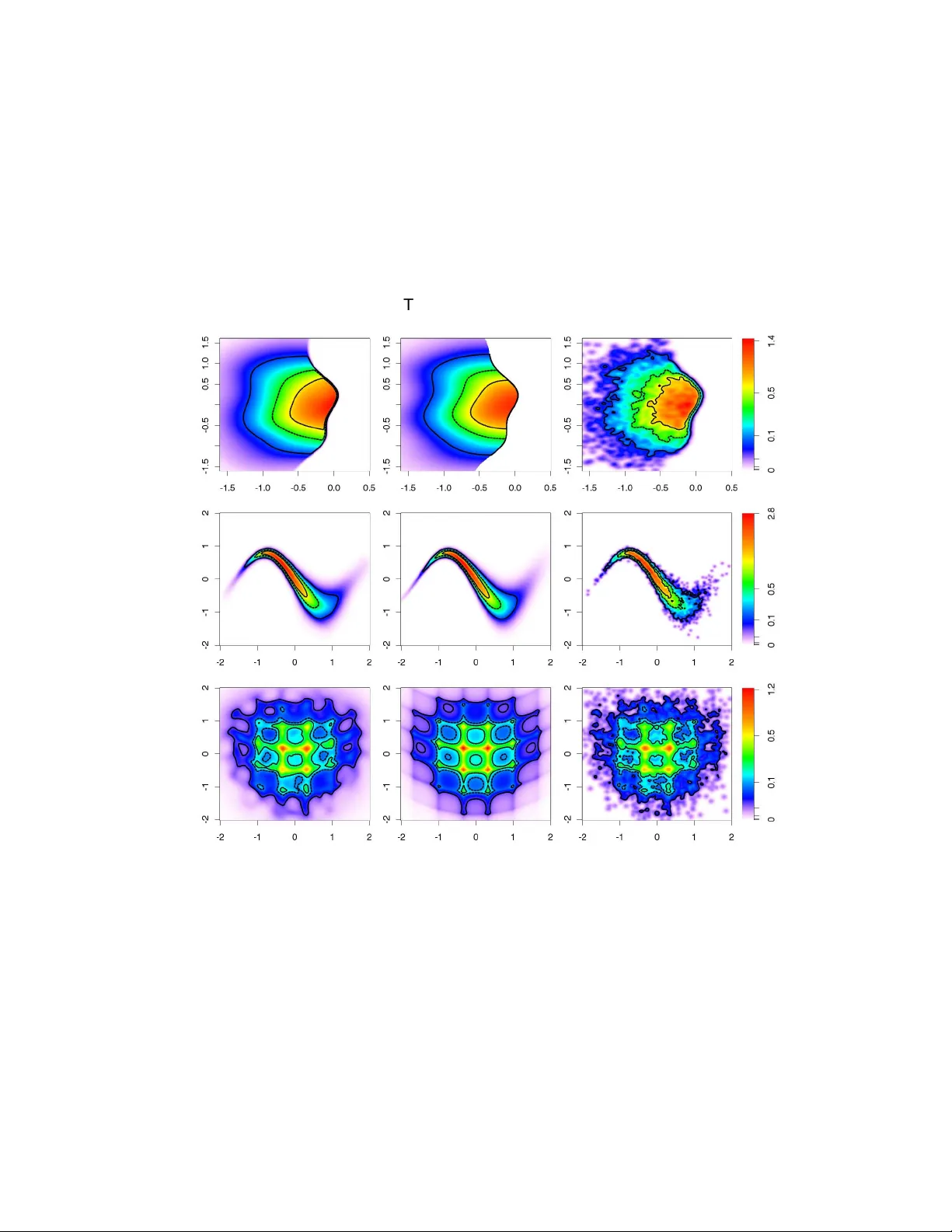
T w o Dimensional Density Estimation using Smooth In ver tible T ransf ormations Ethan Anderes University of California at Ber kele y , USA. Marc Coram Stanf ord University , USA. Summary . W e in vestigate the problem of estimating a smooth inv er tible transformation f when observing independent samples X 1 , . . . , X n ∼ P ◦ f where P is a known measure. W e f ocus on the two dimensional case where P and f are defined on R 2 . W e present a fle xible class of smooth in ver tible tr ansformations in two dimensions with v ar iational equations f or optimizing ov er the classes, then study the prob lem of estimating the transformation f by penalized maximum likelihood estimation. W e apply our methodology to the case when P ◦ f has a density with respect to Lebesgue measure on R 2 and demonstrate improv ements ov er kernel density estimation on three examples . 1. Introduction In this pap er w e in v estigate the problem of estimating the probabilit y distribution of a random v ector X from indep endent copies, X 1 , . . . , X n iid ∼ P ◦ f , where P is a known measure on R d and f is an unknown smooth bijection of R d . W e sp ecif- ically fo cus our atten tion to the tw o dimensional case, where the theory of quasiconformal maps is at our disposal. The estimate is constructed based on the fact that the distribu- tion of X is characterized by f ( X ) ∼ P . Therefore, by attempting to “deform” the data X 1 , . . . , X n b y a transformation f whic h satisfies, f ( X 1 ) , . . . , f ( X n ) iid ∼ P , w e get an estimate of the distribution of X . In what follows we iteratively deform the data tow ard the target distribution P using a gradient ascent t yp e algorithm ov er a class of transformations. F or the remainder of this pap er we reserv e the term ‘transformation’ or ‘deformation’ to refer to a smo oth map whic h is a bijection of R d , i.e. in v ertible and surjectiv e. Deformations hav e b een used in many types of statistical problems. F or example, de- formations are used in spatial statistics for developing nonstationary random fields (see Sampson and Guttorp (1992), Sc hmidt and O’Hagan (2003), Damian et al. (2001), Perrin and Meiring (1999), Iovleff and Perrin (2004), Clerc and Mallat (2003), Anderes and Stein (2008)). Another example is the use of deformable templates for computer vision and med- ical imaging problems (see Y ounes (1999), Joshi and Miller (2000), Dupuis et al. (1998), Ba jcsy and Broit (1982), Ba jcsy et al. (1983), Bo okstein (1989), Amit (1994)). There has 2 E. Anderes and M. Coram also been some work on using transformations to b o ost the efficiency of k ernel densit y es- timates. F or example, in the one dimensional setting Rupp ert and Cline (1994) estimate a transformation of data to a uniform distribution in order to reduce the bias of k ernel density estimation. In a similar manner, data sharp ening tec hniques, dev elop ed by Choi and Hall (1999) and Hall and Minnotte (2002) are used for improving linear density estimates and are av ailable in multiple dimensions. These techniques p erturb the data slightly to pro duce bias reduction. Ho w ev er, the p erturbations need not b e bijective, and so do not represent prop er transformations. Although deformations pro vide a p o w erful mo deling tool, there are man y c hallenges with their practical implemen tation. The in vertabilit y condition, in particular, is one of the main difficulties for constructing flexible classes of transformations and searching within these classes. One of the most common tec hniques for dealing with the inv ertability condition is the use of time v arying v ector field flows for constructing deformations. These vector fields { u t } t ≥ 0 define deformations { f t } t ≥ 0 indexed b y time t ≥ 0 whic h can be used for finding a minimizer of some data dep enden t p enalt y . In this pap er we use a differen t characterization of deformations to construct classes of deformations indexed by a parameter vector θ . Ho w ev er, w e derive a corresp ondence b etw een our parameterization and a time v arying v ector field c haracterization of the corresponding deformations, whereby relating the tw o c haracterizations. Our basic approac h for estimating f is to maximize a p enalized lik eliho o d ov er classes of smo oth transformations. Of course, this requires the existence of a densit y , which will b e guaran teed by mild smo othness conditions on P and f . In tw o dimensions, we develop flexible classes of smo oth inv ertible transformations generated by basis functions, then use the theory of quasiconformal maps to deriv e v ariational formulas that relate p erturbations of a parameterization to p erturbations of the transformations. This, along with a form ula for the rate of change of the likelihoo d allows us to search the parameter space using gradien t-based optimization of a p enalized lik eliho o d. W e finish this section with a more detailed o v erview of the results of this pap er which, w e hop e, will help the reader follow the remainder of the pap er. In section 3, we construct our class of deformations b y using a nonlinear transform of the linear span of a set of basis functions, the co efficients of which generate the parameterization F = { f θ : θ ∈ Θ ⊂ R ∞ } . W e then use known results from quasiconformal maps, outlined in Section 2, to deriv e v ariational relationships that relate a perturbation of the parameters θ to the rate of change of the likelihoo d ` ( θ ) (see Sections 3 and 4). In particular, let θ and d θ b e tw o parameter v ectors suc h that θ + d θ ∈ Θ for all sufficiently small > 0. The results in Section 3.1 sho w that f θ + d θ = f θ + u θ ,d θ ◦ f θ + o ( ) (1) as → 0, where u θ ,d θ is a v ector field which dep ends on b oth θ and d θ . In Section 5, w e presen t some of the algorithmic details for numerically recov ering u θ ,d θ from θ and d θ . W e notice that under mild conditions there exists a partial differential equation which is n umerically solv ed to approximate u θ ,d θ . The v ariational results for f θ are developed primarily to allo w one to perform a gradient- based optimization of a p enalized version of the likelihoo d of X 1 , . . . , X n iid ∼ P ◦ f θ . F or the existence of a likelihoo d one needs sufficient smo othness conditions to ensure P ◦ f θ has a densit y . T o this end, w e assume that P has a strictly p ositiv e differen tiable densit y with resp ect to Leb esgue measure on R 2 . By writing the density as exp H for some differentiable function H : R 2 → R and by assuming f is an orien tation preserving C 1 diffeomorphism Density Estimation Using T ransf ormations 3 of R 2 , P ◦ f has densit y | J f | exp H ◦ f where | J f | is the determinant of the Jacobian of f (alw a ys p ositive by the orientation preserving assumption on f ). Let ` ( θ ) denote the log lik eliho o d of the sample X 1 . . . , X n iid ∼ P ◦ f θ so that ` ( θ ) = n X k =1 log | J θ f ( X k ) | + H ◦ f θ ( X k ) . (2) No w define the rate of c hange of the log likelihoo d at θ in the direction d θ by ˙ ` [ θ ]( d θ ) := lim → 0 ` ( θ + d θ ) − ` ( θ ) when it exists. In Section 4 we derive the following formula for ˙ ` ˙ ` [ θ ]( d θ ) = n X k =1 div u θ ,d θ ( Y k ) + h u θ ,d θ ( Y k ) , ∇ H ( Y k ) i (3) where Y k = f θ ( X k ), h· , ·i is dot product in Euclidean space, u θ ,d θ is the vector field found in (1), and div u θ ,d θ is the divergence of u θ ,d θ . A heuristic interpretation of (3) can b e given by viewing the t w o terms as b eing comp etitors for maximizing the rate of increasing of the log-likelihoo d. In particular, let f b e a prop osed transformation of the data so that f ( X 1 ) , . . . , f ( X n ) are appro ximately distributed as P . Consider attempting a small p erturbation b y a vector field u , f + u ◦ f + o ( ), that increases the log-lik eliho o d. T o find a goo d p erturbation one w an ts to maximize the t wo terms: div u ( f ( X k )) and h u ( f ( X k )) , ∇ H ( f ( X k )) i , for k = 1 . . . , n . Notice that div u ( f ( X k )) measures lo cal expan- sion at f ( X k ) so that large v alues of div u ( f ( X k )) correp ond to an expansion the region surrounding f ( X k ). In contrast, the term h u ( f ( X k )) , ∇ H ( f ( X k )) i is large when the vector field gravitates to w ard the modes of the densit y of P . This gives an expansion-con traction comp etition for increasing the rate of change of the log-lik eliho o d and by suitably balancing these t w o comp eting terms one gets the b est rate of increase of the log-likelihoo d. In Section 5 we use equations (1) and (3) to perform a gradient ascent of a p enalized v ersion of the log likelihoo d. By truncating the parameter space θ N := ( θ 1 , . . . , θ N ), the gradien t ascen t path { θ N t } t ≥ 0 is c haracterized b y d dt θ N t = ∇ ` ( θ N t ) − λ ∇ J ( θ N t ) where J is a regularization p enalt y , λ ≥ 0 is a tuning parameter and ∇ ` ( θ N ) = ˙ ` [ θ N t ]( e 1 ) . . . ˙ ` [ θ N t ]( e N ) , where e 1 , . . . , e N are the standard basis vectors for R N . The n umerical details for computing ∇ ` ( θ N ) and implementing the gradient-based optimization are also given in Section 5. Finally , in Section 6, we present a series of sim ulation experiments. Our estimates, which are constructed using a F ourier basis to generate the parameterization f θ , compare fav orably to a k ernel densit y estimate. 2. Quasiconformal maps and V ariations W e briefly review some results from the theory of quasiconformal maps. F or more a complete treatmen t see Ahlfors (2006), Krushk al’ (1979), La wryno wicz (1983), Lehto and Virtanen 4 E. Anderes and M. Coram (1965). The main result of quasiconformal theory used in this pap er is the c haracterization of quasiconformal maps by another function called a complex dilatation. Complex dilatations are imp ortan t for t w o reasons. First, they are only required to b e measurable and b ounded ab o v e by some k < 1, which makes it easy to construct classes of smo oth transformations. Secondly , there is a constructible corresp ondence b et w een the p erturbation of a complex dilatation and the p erturbation of the corresp onding transformation. This is used to derive the rate of c hange of the likelihoo d (see equation (3)) as one v aries a parameterization of smo oth transformations. F or a C 1 diffeomorphism f define ∂ f := 1 2 ∂ ∂ x − i ∂ ∂ y f , ∂ f := 1 2 ∂ ∂ x + i ∂ ∂ y f . The complex dilatation of f , denoted µ f or just µ , is defined as µ := ∂ f /∂ f . The v alue of the complex dilatation at a p oint z , µ ( z ), c haracterizes the infinitesimal ellipse ab out z , whic h gets mapp ed to a infinitesimal circle under the image of f . In particular, the eccen tricit y of the ellipse is given by 1+ | µ | 1 −| µ | and the inclination is given by arg ( − µ/ 2). W e will sometimes use the alternativ e notation f z , f z for ∂ f , ∂ f when doing so makes an equation more readable. By generalizing to weak deriv atives for ∂ f and ∂ f , one can extend the definition of the complex dilatation µ f := ∂ f /∂ f . A quasiconformal map is defined to b e a homeomorphism f with lo cally square in tegrable weak deriv atives suc h that ess sup | µ f | < 1. This condition on µ f is equiv alen t to requiring that the eccentricities of the lo cal ellipses characterized by µ f b e a.e. b ounded. W e now hav e the following Theorem found in Ahlfors (2006), page 57. Theorem 1. F or any me asur able µ with k µ k ∞ < 1 ther e exists a unique quasic onformal mapping f µ with c omplex dilatation µ that le aves 0 , 1 , ∞ fixe d. W e also hav e the nice fact that all quasiconformal maps with a given dilatation are found b y p ost comp osing the unique map f µ in Theorem 1 with a conformal map. In this w ay , an y quasiconformal map f : C → C with dilatation µ has the form af µ + b for a, b ∈ C . The usefulness of this characterization is seen in the construction of classes of quasiconformal maps in Section 3. W e finally mention that if µ is kno wn to b e H¨ older con tin uous, the map f will b e a C 1 diffeomorphism. 2.1. The dependence of f µ on µ Besides characterizing quasiconformal maps, the other imp ortant prop erty of the complex dilatation is that f µ dep ends differen tially on µ so that a small p erturbation µ + ν leads to a vector field perturbation f µ + u ◦ f µ + o ( ) of f µ . An in tegral equation then relates ν and the v ector field u . T o b e more precise supp ose { µ t } t ≥ 0 is a class of deformations suc h that µ t + = µ t + ν t + γ ( t, ) where γ ( t, ) , ν t ∈ L ∞ , k µ t k ∞ < 1, and k γ ( t, ) k ∞ → 0 as → 0. Then b y Theorem 5, page 61 of Ahlfors (2006), f µ t + = f µ t + u t ◦ f µ t + o ( ) , (4) uniformly on compact subsets where, u t ( ζ ) := − 1 π Z Z L µ t ν t ( z ) R ( z , ζ ) dxdy , (5) Density Estimation Using T ransf ormations 5 for R ( z , ζ ) = ζ ( ζ − 1) z ( z − 1)( z − ζ ) , L µ ν := n ν 1 −| µ | 2 ∂ f µ ∂ f µ o ◦ ( f µ ) − 1 and z = x + iy . By H¨ older’s inequalit y the in tegral indeed exists when L µ t ν t ∈ L ∞ . By prop erties of the in tegral (5) the v ector field u t satisfies ∂ u t = L µ t ν t , u t (0) = u t (1) = 0 , (6) in the distributional sense when L µ t ν t ∈ L p for some p > 2 (see Lemma 3, page 53 of Ahlfors (2006)). W e use (6) to approximate the integral (5) in Section 5. Finally , one of the consequences of (4) is that for sufficiently smo oth { u t } t ≥ 0 the deter- minan t of the Jacobian of f µ t at x ∈ R 2 , denoted | J t ( x ) | , exists and satisfies d dt | J t ( x ) | = | J t ( x ) | div u t ◦ f t ( x ) . (7) F or references see Theorem 3.1.2 of Hille (1969) or Corollary 3.1 of Hartman (2002) (page 96). It is (7) that gives the rate of change of the likelihoo d ˙ ` [ θ ]( d θ ) in equation (3). 3. Classes of Quasiconformal maps T o ensure that P ◦ f is a genuine probability measure, one must require that the C 1 dif- feomorphism, f , be inv ertible. It is this nonlinear condition that is the main obstacle for constructing a rich class of transformations, { f θ : θ ∈ Θ ⊂ R ∞ } . In this section, to ov er- come this difficulty , we use the flexibilit y of complex dilatations µ to construct our class of transformations. By defining a set of basis functions ϕ k : C → C for k = 1 , 2 , . . . w e formally construct a class of complex dilatations, M := ( µ = ϕ 1 + | ϕ | : ϕ = X k c k ϕ k , c k ∈ R ) . (8) The reason for introducing the transformation ϕ 7→ ϕ 1+ | ϕ | is to remo ve an y restriction, b esides measurabilit y and b oundedness, on the linear span ϕ = P k ϕ k to define a class of quasiconformal maps. Indeed, b y Theorem 1, for any complex dilatation µ ∈ M with ϕ = P k c k ϕ k ∈ L ∞ , there exists a unique quasiconformal map f θ = af µ + b , where θ = ( a 1 , a 2 , b 1 , b 2 , c 1 , c 2 , . . . ), a = a 1 + ia 2 6 = 0 and b = b 1 + ib 2 . No w w e construct the full class F of transformations, F := { f θ : θ ∈ Θ ⊂ R ∞ } , where Θ is the set of parameter v alues for which P k c k ϕ k ∈ L ∞ and a 6 = 0. 3.1. V ar iational Relationship between θ and f θ One of the main comp onents of the gradien t ascent algorithm is the computation of the v ector field p erturbation of f θ that results from a small change of the parameter v ector θ + d θ . W e start this section b y studying how the perturbation θ + d θ propagates to µ , then finish with a deriv ation of the expansion f θ + u θ ,d θ ◦ f θ + o ( ). Supp ose ϕ, dϕ ∈ L ∞ are b oth members of the linear span of { ϕ k } k ∈ N . W e start by sho wing that p erturbing ϕ b y ϕ + dϕ results in µ + ν + o ( ) where ν = dϕ 2 + | ϕ | 2(1 + | ϕ | ) 2 − dϕ ϕ 2 2 | ϕ | (1 + | ϕ | ) 2 (9) 6 E. Anderes and M. Coram where, for the rest of this pap er, the second term of the righ t hand side of (9) is understo o d to b e zero at the p oints z such that ϕ ( z ) = 0. T o b e more precise, let µ ϕ = ϕ 1+ | ϕ | and ν ϕ ( dϕ ) := ν as in (9). Supp ose ϕ = P ∞ k =1 c k and dϕ = P ∞ k =1 dc k ϕ k are complex functions in L ∞ with real co efficien ts { c k } k ≥ 1 and { dc k } k ≥ 1 . Then µ ϕ + dϕ = µ ϕ + ν ϕ ( dϕ ) + γ ( ) (10) where ν ϕ ( dϕ ) , γ ( ) ∈ L ∞ and k γ ( ) k ∞ → 0 as → 0. T o see wh y , let T ( z ) = z 1+ | z | , where z = x + iy and notice that ∂ T ( z ) /∂ x and ∂ T ( z ) /∂ y are contin uous on C and satisfy ∂ T ( z ) ∂ x = 1 1 + | z | − x z | z | (1 + | z | ) 2 ∂ T ( z ) ∂ y = i 1 + | z | − y z | z | (1 + | z | ) 2 . where the last term is 0 when z = 0. Therefore directional deriv ativ e ∂ u T , in the direction u ∈ C , exists and is contin uous on C for any fixed u = u 1 + iu 2 and is giv en b y ∂ u T ( z ) = u 1 ∂ T ( z ) ∂ x + u 2 ∂ T ( z ) ∂ y = u 1 + | z | − uz + uz 2 z | z | (1 + | z | ) 2 = u 2 + | z | 2(1 + | z | ) 2 − u z 2 2 | z | (1 + | z | ) 2 where the last term is 0 when z = 0. Therefore the map T has a F r´ ec het deriv ativ e T 0 z ( u ) := ∂ u T ( z ) and b y the mean v alue theorem (see Dieudonn´ e (1960)) T ( ϕ ( z ) + dϕ ( z )) − T ( ϕ ( z )) − T 0 ϕ ( z ) ( dϕ ) ≤ | dϕ ( z ) | sup ξ ∈ S T 0 ξ − T 0 ϕ ( z ) for a fixed z ∈ C , where S is the line connecting ϕ ( z ) + dϕ ( z ) and ϕ ( z ), and k · k is the standard op erator norm on the space of con tin uous linear mappings from R 2 to R 2 . Now sup ξ ∈ S T 0 ξ − T 0 ϕ ( z ) ≤ sup | ξ − ϕ ( z ) |≤ B T 0 ξ − T 0 ϕ ( z ) where k dϕ k ∞ = B . The last term conv erges to zero uniformly in z ∈ C as → 0 since ϕ ( z ) is b ounded and T 0 η is uniformly con tin uous on compact domains. Therefore T ( ϕ + dϕ ) = T ( ϕ ) + T 0 ϕ ( dϕ ) + γ ( ) where k γ ( ) k ∞ → 0 as → 0, whic h gives (10). Finally notice | ν ϕ ( dϕ ) | = | T 0 ϕ ( dϕ ) | ≤ k dϕ k ∞ / (1 + | ϕ | ) ≤ k dϕ k ∞ < ∞ . No w we can com bine all the p erturbation results to derive v ariational relationship b e- t w een the coefficients and the maps. Supp ose θ = ( θ 1 , θ 2 , . . . ) and d θ = ( dθ 1 , dθ 2 , . . . ) are tw o parameter vectors suc h that θ + d θ ∈ Θ for all sufficiently small > 0. Let ϕ = P ∞ k =4 θ k ϕ k , dϕ = P ∞ k =4 dθ k ϕ k , µ = ϕ 1+ | ϕ | , and ν defined by (9). Also let da = dθ 1 + idθ 2 Density Estimation Using T ransf ormations 7 and similarly db = dθ 3 + idθ 4 . The following display summarizes how the pe rturbation of θ b y d θ propagates through f θ : θ + d θ 7→ ϕ + dϕ a + da b + db by (10) 7→ µ + ν + o ( ) a + da b + db by (4) 7→ f µ + u ◦ f µ + o ( ) a + da b + db where u ◦ f µ ( ζ ) = − 1 π R R L µ ν ( z ) R ( z , f µ ( ζ )) dxdy and L µ ν = n ν 1 −| µ | 2 ∂ f µ ∂ f µ o ◦ ( f µ ) − 1 . T o get the p erturbations in the form f θ + d θ = f θ + u θ ,d θ ◦ f θ + o ( ) we simplify equation f θ + d θ = ( a + da ) f µ + u ◦ f µ + o ( ) + b + db = f θ + ( au ◦ f µ + da f µ + db ) + o ( ) . Notice u ◦ f µ ( ζ ) = − 1 π Z Z ν ( z ) R ( f µ ( z ) , f µ ( ζ ))( ∂ f µ ( z )) 2 dxdy = − 1 π Z Z ν ( z ) ( b − f θ ( ζ ))( a + b − f θ ( ζ )) ( f θ ( z ) − f θ ( ζ ))( b − f θ ( z ))( a + b − f θ ( z )) ( ∂ f θ ( z )) 2 a dxdy = − 1 aπ Z Z L θ ν ( z ) ( b − f θ ( ζ ))( a + b − f θ ( ζ )) ( z − f θ ( ζ ))( b − z )( a + b − z ) dxdy , where L θ ν := n ν 1 −| µ | 2 ∂ f θ ∂ f θ o ◦ ( f θ ) − 1 . Therefore, finally , we hav e f θ + d θ = f θ + u θ ,d θ ◦ f θ + o ( ) (11) where u θ ,d θ ( ζ ) = db + da a ( ζ − b ) − 1 π Z Z L θ ν ( z ) ( b − ζ )( a + b − ζ ) ( z − ζ )( b − z )( a + b − z ) dxdy . (12) If w e ha v e the nice situation that L θ ν ∈ L p for some p > 2 it can b e shown that ∂ u θ ,d θ = L θ ν in the distributional sense where u θ ,d θ ( b ) = db and u θ ,d θ ( a + b ) = da + db . 4. Rate of Chang e of the Likelihood W e now return to the observ ation scenario where we hav e iid observ ations X 1 , . . . , X n from the measure P ◦ f θ where P is a known measure on R 2 and f θ is known only to b e a mem b er of the class of inv ertible transformations F given by (3). W e also supp ose that P has a strictly p ositive differentiable densit y with resp ect to Leb esgue measure on R 2 and write the density exp H for some differentiable function H : R 2 → R . Since H is assumed to b e known, the likelihoo d of the observ ations X 1 , . . . , X n , as a function of θ ∈ Θ, is giv en by (2). Let J θ + d θ x ) | denote the determinan t of the Jacobian of the map f θ + d θ ev aluated at x ∈ R 2 . Notice that equations (11) and (7) give d d h log J θ + d θ ( x ) i =0 = div u θ ,d θ ◦ f θ ( x ) (13) d d h H ◦ f θ + d θ ( x ) i =0 = u θ ,d θ ◦ f θ ( x ) , ∇ H ◦ f θ ( x ) (14) 8 E. Anderes and M. Coram for all x ∈ R 2 where u θ ,d θ is given by equation (12) and · , · denotes dot pro duct in R 2 . Therefore ˙ ` [ θ ]( d θ ) := d d h ` ( θ + d θ ) i =0 = d d " n X k =1 log | J θ + d θ ( X k ) | + H ◦ f θ + d θ ( X k ) # =0 = n X k =1 div u θ ,d θ ( Y k ) + u θ ,d θ ( Y k ) , ∇ H ( Y k ) , where Y k = f θ ( X k ) and u θ ,d θ is given by (12). Notice that this giv es formula (3) giv en in the in tro duction. Finally we mention that ˙ ` [ θ ]( · ) is linear ov er the reals so that ˙ ` [ θ ]( d θ ) = X k dθ k ˙ ` [ θ ]( e k ) where θ = P k θ k e k and d θ = P k dθ k e k where where e k = (0 , . . . 0 , 1 , 0 , . . . ) with the non- zero elemen t at the k th index. 5. Algorithmic details In this section we discuss the algorithmic details for a gradient ascent of the likelihoo d ` ( θ ). In our implementation of the algorithm, w e slightly adjusted these techniques by using quasi-Newton up dates instead of gradient ascent up dates. Ho w ev er, the essen tial comp onen ts of the algorithm are still captured by gradient ascen t while allowing succinct exp osition. Therefore, w e reserv e the details of the quasi-Newton updates for the next section. The gradient ascent will b e done b y truncating the parameter space θ N := ( θ 1 , . . . , θ N ) and using (3) to write, ∇ ` ( θ N ) = ˙ ` [ θ N ]( e 1 ) . . . ˙ ` [ θ N ]( e N ) = n X k =1 div u 1 ( Y k ) + h u 1 ( Y k ) , ∇ H ( Y k ) i . . . div u N ( Y k ) + h u N ( Y k ) , ∇ H ( Y k ) i , (15) where u 1 := u θ N ,e 1 , . . . , u N = u θ N ,e N and Y k = f ( X k ). Gradient ascen t is then written as a solution to, d dt θ N t = ∇ ` ( θ N t ) − λ ∇ J ( θ N t ) , (16) where J is a regularization penalty . The most difficult part of of this algorithm is solving u 1 , . . . , u N at each step in a discretization of (16). W e start this section with a detailed discussion of this problem and finish with a few commen ts on the recursive nature of the gradien t ascen t. T o find the v ector fields u 1 , . . . , u N in (15) one needs compute the singular in tegral (12). When ν has compact supp ort, the integral (12) has the form ( P L θ ν )( ζ )+(linear function of ζ ) where P h ( ζ ) := − 1 π R R h ( z ) / ( z − ζ ) dxdy is the Cauch y T ransform. After a simple scal- ing, one has av ailable the computational techniques found in Daripa and Mashat (1999) for computing the Cauch y T ransform ov er the unit disk. In particular, suppose h is a Density Estimation Using T ransf ormations 9 function with compact support in Ω and let c b e a constant such that c ≥ | z | for all z ∈ Ω. Then h c ( z ) := h ( cz ) has supp ort in the unit disk D and P h ( c ζ ) = cP h c ( ζ ) = − c π R R D h c ( z ) / ( z − ζ ) dxdy for all ζ ∈ D . No w one can use Diripa and Mashat’s metho d to appro ximate R R D h c ( z ) / ( z − ζ ) dxdy . Finally one needs to find the linear correction to P L θ ν for the integral (12). This is accomplished by the t wo necessary conditions u θ ,d θ ( a ) = da and u θ ,d θ ( a + b ) = da + db . A second approac h for approximating u θ ,d θ is to solv e the nonhomogeneous Cauch y- Riemann equations ∂ u θ ,d θ = L θ ν . The solution is only unique up to additive analytic functions, ho wev er, if it is kno wn that L θ ν ∈ C 2 0 then P L θ ν ∈ C 2 and ∂ P L θ ν ∈ L 2 (see Lemma 2, page 52 of Ahlfors (2006)). Therefore any contin uous solution to ∂ u θ ,d θ = L θ ν whic h satisfies ∂ u θ ,d θ ∈ L 2 is an additiv e constant difference of P L θ ν . Therefore one can find u θ ,d θ b y solving the nonhomogeneous Cauc hy-Riemann equation ∂ u θ ,d θ = L θ ν with free b oundary conditions on ∂ Ω, where Ω is the supp ort of L θ ν . In our implementation of the algorithm the Diripa and Mashat’s metho d suffered from some instabilities. W e instead used an ad-ho c metho d for trying to inv ert the equation ∂ u d θ = L θ ν b y representing u θ ,d θ b y a latent complex function w such that u = ∂ w (this is basically a stream function and p otential function represen tation of a v ector field with the co ordinates switched) then using the fact that 4 ∂ ∂ = ∆, the Lapacian operator, we used a fast P oisson solver in Ma tlab to inv ert ∆ w = 4 L θ ν . One drawbac k to this tec hnique is that it p otentially differs from P L θ ν by an additiv e analytic function. In the cases we studied the magnitude of the analytic difference w as small enough to b e ignored. How ever, w e would prefer Daripa and Mashat’s metho d but leav e it’s prop er implementation to more adept n umerical programmers. One particularly attractive feature of the algorithm is its recursive nature. Supp ose at step m of a discretized gradient ascent one has f θ m and f θ m z ev aluated on a dense grid. W e sho w how to find f θ m +1 and f θ m +1 z at step m + 1. T o mak es the following formulas more readable let µ θ m = ϕ θ m 1+ | ϕ θ m | b e the complex dilatation of f θ m , where ϕ θ m = P k ≥ 4 ( θ m ) k ϕ k is giv en b y the basis expansion in (8). The gradient up date is θ m +1 = θ m + d θ m where d θ m = ( ˙ J [ θ m ]( e 1 ) , ˙ J [ θ m ]( e 2 ) , . . . ) . Remem b er that for eac h j ≥ 4, ˙ J [ θ m ]( e j ) = n X k =1 div u j ( Y k ) + h u j ( Y k ) , ∇ H ( Y k ) i , where, Y k = f θ m ( X k ), ∂ u j = L θ m ν j and ν j is giv en b y ν j = ϕ j 2 + | ϕ θ m | 2(1 + | ϕ θ m | ) 2 − ϕ j ( ϕ θ m ) 2 2 | ϕ θ m | (1 + | ϕ θ m | ) 2 . Notice that computing L θ m ν j can b e accomplished b y simply deforming the graph of ν j 1 −| µ θ m | 2 f θ m z f θ m z b y f θ m . Now f θ m +1 := f θ m + u θ m ,d θ m ◦ f θ m and using the comp osition rule for ∂ and fact that ∂ u θ m ,d θ m = L θ m ν w e get the follo wing up date for f θ m +1 z f θ m +1 z = f θ m z 1 + u θ m ,d θ m z ◦ f θ m + ν µ θ m 1 − | µ θ m | 2 ! where ν = P k ≥ 4 ( d θ m ) k ϕ k . 10 E. Anderes and M. Coram x Fig. 1. Panel of Density Estimates: The true sampling density is shown in the central column; in the left and right columns are density estimates based on the same sample of 10,000 points using respectively the def or mation-based methods of this paper and kernel density estimates. There is one row per e xample: halfg, stroke, waffle. As indicated by the colorbar , the scale f or the heatmaps is non- linear to accentuate diff erences in low-density regions (a square-root transf orm is used, consistent with Hellinger distance). A solid line is dra wn at the contours of the density that capture 95% of the mass; the 50% line is dashed, and the 25% line is dash-dotted. Density Estimation Using T ransf ormations 11 T able 1. T able of the average integrated squared errors, sum- marized across six independent realizations. Av erages (and parenthetical standard de viations) are repor ted times 10 4 Sample Size Case Metho d 10 , 000 1 , 000 100 Halfg deformation 59 (4) 109 (19) 325 (83) k ernel 190 (8) 409 (34) 880 (181) Strok e deformation 24 (8) 122 (30) 909 (209) k ernel 157 (18) 642 (81) 2354 (454) W affle deformation 64 (5) 222 (30) 674 (30) k ernel 74 (5) 259 (26) 662 (49) 6. Simulation Experiments T o inv estigate the quality of the density estimates obtained by the deformation metho d w e p erformed a series of sim ulation exp erimen ts. W e first give an ov erview of the results; details are explained afterw ard. Data sets of size 100, 1000, and 10,000 were generated indep enden tly from three distributions that we call halfg, stroke, and waffle. Eac h example is intended to demonstrate different prop erties of our estimator; the examples, and the results are illustrated in Figure 1. The halfg example was chosen to highlight the ability of the deformation metho d to 1) adapt to sharp edges of the density 2) utilize qualitativ e knowledge ab out the form of the density , namely through the use of a softened half-normal as the target density . The strok e example, in which a normal density is stretc hed out into an “S” with the thickness v arying along the length, is intended to test the abilit y of the deformation to capture the o verall structure well enough to extend mass into the tails appropriately . The w affle example tests the estimates p erformance in a complex, bumpy case. Both the stroke and the waffle examples use a radially symmetric biv ariate Gaussian distribution with mean 0 as the target. F or stroke, the target has standard deviation 0.05; for waffle, the target has standard deviation 0.5. F rom these ch oices w e find that the metho d can successfully reconstruct the long thin stroke density by “stretching” a small target, and can also match the complex w affle pattern on to a mo derate target. F or eac h data set, the optimal p enalty parameter λ was c hosen to minimize the integrated square error (ISE) difference b etw een the densit y estimated for that λ and the true sampling densit y . The minimal ISE was recorded and compared with the minimum ISE achiev ed b y k ernel density estimation at the optimal bandwidth. T o determine the sampling v ariability of the findings, this was rep eated six times for each example. These results, as w ell as results for Hellinger and L 1 distance measures, are tabulated in T ables 1, 2, and 3. Examples of the estimates ac hiev ed on data sets of 10,000 are shown in Figure 1. 6.1. Sampling Densities In this subsection we giv e the detailed recip es for the sampling distributions and target densities used in the examples. Halfg: Let x = ( x 1 , x 2 ) t , let Ψ( x ) = ( x 1 + h ( x 2 ) , x 2 ) t , where h ( u ) = sin(5 u ) / 15 − u tanh( u ) / 3. The data were generated by sampling from a symmetric biv ariate normal with 12 E. Anderes and M. Coram T able 2. T able of the av erage Hellinger-distance errors, summa- rized across six independent realizations. A verages (and paren- thetical standard de viations) are repor ted times 10 4 Sample Size Case Metho d 10 , 000 1 , 000 100 Halfg deformation 863 (17) 1160 (43) 1915 (250) k ernel 1881 (19) 2718 (54) 3860 (236) Strok e deformation 443 (33) 992 (110) 2601 (187) k ernel 1083 (32) 2048 (53) 3800 (285) W affle deformation 1021 (31) 1826 (68) 3002 (116) k ernel 1193 (24) 2105 (66) 3149 (78) T able 3. T able of the a ver age L1-distance errors, summar ized across six independent realizations. Av erages (and parenthetical standard de viations) are repor ted times 10 4 Sample Size Case Metho d 10 , 000 1 , 000 100 Halfg deformation 544 (46) 955 (93) 1 808 (250) k ernel 1385 (35) 2382 (115) 3980 (475) Strok e deformation 487 (71) 1124 (120) 3104 (259) k ernel 1268 (53) 2572 (124) 5018 (442) W affle deformation 1535 (48) 2813 (136) 4814 (139) k ernel 1726 (38) 3153 (113) 4969 (117) Density Estimation Using T ransf ormations 13 standard deviation 1 / 2, rejecting p oints in the right half plane, and applying the transfor- mation Ψ to the remaining points. In effect, then, the density of the observed p oints is a deformed half-normal. Notice that the indicator introduces a smo othly curved sharp edge to the densit y: 2(1 / √ 2 π ) 2 (1 / 2) 2 exp( − 1 / 8(( x 1 − h ( x 2 )) 2 + x 2 2 ) 1 x 1 − h ( x 2 ) ≤ 0 F or the halfg example, instead of using a standard Gaussian as our target we used a softened half-normal; the softening was done so that the target would b e a contin uously differen tiable densit y to facilitate optimization, y et still describe a half-normal-like distribu- tion. Sp ecifically , the target distribution is describ ed by indep endently dra wing X 2 from a normal with mean 0 and standard deviation 1 2 , and X 1 from the mixture of half-normals with densit y γ [2 φ σ + ( x ) I x ≥ 0 ] + (1 − γ )[2 φ σ − ( x ) I x< 0 ], where σ − = 1 2 , σ + = 1 50 , γ = (1 + σ − /σ + ) − 1 , and φ σ is the densit y of a normal with mean 0 and standard deviation σ . Str oke: Let Ψ( x ) = x 1 / 2 , 1 20 (3 + 2 tanh( x 1 )) x 2 − 4 5 sin( x 1 ) t . The samples are generated b y sampling X = ( X 1 , X 2 ) t as a pair of independent standard normals, and applying transformation Ψ. The target density w as taken to b e a mean 0 symmetric biv ariate normal with standard-deviation 0 . 05. Waffle: Let Ψ( x ) = 2 3 x 1 + sin(2 π x 1 ) / (2 π s ) , x 2 + cos(2 π x 2 ) / (2 π s ) + ( x 1 / 3) 2 t , where we tak e s = 1 2 . The samples are generated by sampling X = ( X 1 , X 2 ) t as a pair of indep endent standard normals, and applying transformation Ψ. The target densit y was taken to b e a mean 0 symmetric biv ariate normal with standard-deviation 0 . 5. 6.2. Basis Functions ϕ k and P enalty J ( θ ) . Here we define the basis functions ϕ k , in (8), and the regularization p enalty J , in (16), used for our simulations. T o motiv ate our choice of basis functions ϕ k , we note the F ourier represen tation of L 2 functions on [ − L, L ] 2 : ϕ ( x + iy ) = X k 1 ,k 2 ∈ Z ( a k 1 ,k 2 + ib k 1 ,k 2 ) e i 2 π ( k 1 x + k 2 y ) / 2 L = X k 1 ,k 2 ∈ Z a k 1 ,k 2 e i 2 π ( k 1 x + k 2 y ) / 2 L + X k 1 ,k 2 ∈ Z b k 1 ,k 2 ie i 2 π ( k 1 x + k 2 y ) / 2 L , for real co efficien ts a k 1 ,k 2 , b k 1 ,k 2 . These F ourier basis functions are smoothly truncated to zero outside of the disk of radius L by m ultiplying each basis function b y T ( x, y ) = [1 − (( x/L ) 2 + ( y /L ) 2 ) 4 ] 1 { x 2 + y 2
Original Paper
Loading high-quality paper...
Comments & Academic Discussion
Loading comments...
Leave a Comment