Bounded Mean-Delay Throughput and Non-Starvation Conditions in Aloha Network

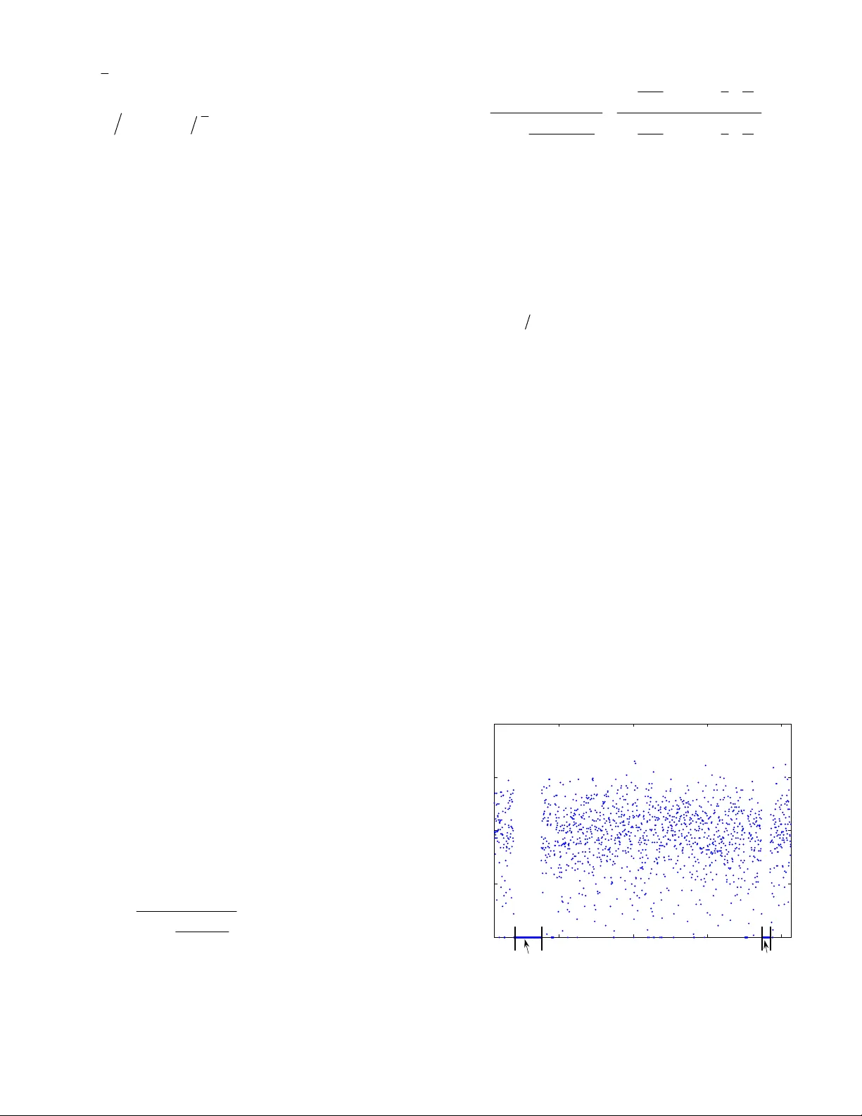
7/14/2008 1 Bounded Mean-Delay Throughput and Non-Starvation Conditions in Aloha Network Soung Chang Liew, Senior Member, IEEE , Ying Jun (Angela) Zhang, Member, IEEE , Da Rui Chen, Student Member, IEEE The Department of Information Engineering, The Chinese University of Hong Kong Shatin, New Territory, Hong Kong Email: { scliew, yjzhang, drchen}@ie.cuhk.edu.hk Abstract — Prior investigations on the Aloha network has primarily focused on its system throughput. Good system thr oughput, however , does not automatically translate to good delay performance for the end users. Neither is fairness guaranteed: s ome users may s tarve while others hog the system. This p aper establishes the con ditions for bounded mean queuing delay and non-star ved operation of the slotted Aloha network. We focus on the performance w hen collisions of packets are resolved us ing an ex ponential backoff protocol. For a non-saturated networ k, we find that bounded mean-delay and non- starved operation can be guaran teed only if the offered load is limited to below a quantity calle d “safe bounded-mean-delay (SBM D) throughput”. The SBMD throughput c an be much lower than the saturation system throughput if the bac koff factor r in the exponential backoff algorithm is not properly set. For example, it is well known that the maximum throughput of the Aloha netw ork is 1 0.3679 e − = . However, for 2 r = , a value assumed in many prior investigations, the SBMD throughput is only 0.2158, a drastic penalty of 41% relative to 0.3679. Fortunately, using 1.3757 r = allows us to obtain SBMD throughput of 0.3545, less than 4% away from 0.3679. A general conclusion is that the system parameters can sign ificantly affect the delay an d fairness performance of the Aloh a network. This paper provides the analytical fram ework and e xpressions for tuning r and other system parameters to achieve good delay and non-starved operation. Index Terms —Access protocols, network performance, wireless LAN. 1. Introduction he Aloha network has been studied extensively since the pioneer work by Abramson [1] . Prior work on the Aloha network has primarily focused on its overall system throughput. To achieve good system throughput, the transmission probabilities of the nodes must be adjusted dynamically according to the contention inte nsity in the network. An exponenti al backoff protocol can serve this purpose rather effectivel y [2]. Good system throughput, however, does not aut omaticall y translate to acceptable performance from the end user perspective. For example, if a real-time app lication such as a voice call is running on top the Aloha network, del ay performance is import ant. Even if the end application is not a real-tim e application, there is also the fairness issue, wherei n some nodes in the Aloha network are starved while other nodes enjoy good service. For example, for a TCP application, starvat ion could cause its TCP connection to terminate halfway. This paper is devoted to the st udy of how to ensure good delay and non-starved performance in a slot ted Aloha network operated with an exponential backoff prot ocol. In particul ar, we are interested in the setti ng of system param eters to attain not just good overall system throughput, but also good delay and fairness performance. Within this context, this paper has two major contributions: 1. We establish an analytical framework for the study of queuing delay and starvation i n the Aloha network. 2. Based on the analytical framework, we derive the dependency of delay and non-starvation on t he system param eters. With respect to contribution 1, we unit e the concepts of bounded mean-delay perform ance and non-starvation, arguing that the conditions giving rise to them are one of the same i n a non- saturated Aloha network: namely, the service time at the heads of queues must be bounded. We find that t he “saturation throughput”, a performance m etric of focus in ma ny prior studies, is not a sound measure of performance if we care about delay and non-st arved operation. In particular, to achieve good del ay and non-starved operation, the offered load must be below an other quantity called “safe-bounded-mean-delay (SB MD) throughput”, which can be substantiall y lower than the saturation t hroughput. In establishing our analytical framework, we find th at the delay analysis is much trickier than the saturat ion-throughput analysi s in prior work. To better bring out the subtl eties involved, we decom pose our analysis into three steps: (i) a glob al analysis that cap tures the interactio n among nodes; (ii ) a local analysis that captures the dynam ic within a node; (iii) a coupling analysis that integrates (i) and (ii) into a coherent whole. Steps (ii) and (iii) in the delay analysis, in particular, are a lot more involved than steps (ii) and (iii) in the saturation analysis. With respect to contribution 2, we show that del ay and non- starvation can be very sen sitive to the system parameters; m uch more so than the saturati on throughput is. For example, it is well known that the maxim um sat uration throughput of a large slot ted Aloha network with m any nodes is 1 0.3679 e − = . An exponential backoff factor of 2 (see Section 2.1 for the definition of t he backoff factor) was com monly assum ed in ma ny prior studies [3] T 7/14/2008 2 [4]. It can achieve a saturation throughput of 0.3466 [2]. Thus, backoff factor of 2 is quite satisfacto ry when it comes to saturation throughput performance. However, if we desire bounded m ean- delay and non-starved performance, we m ust lim it the system offered load to below 0.2158, a drastic penalty of 41% with respect to the maxi mum t hroughput. Fortunately, i f instead of 2, we use a backoff factor of 1.3757, t he sustainable offered load can reach 0.3545, very close to th e maxim um throughput. This paper will present many other intricate relationsh ips between system parameters and sy stem operation and perform ance. Related Work Most prior investigat ions on the Aloha network (e.g., [2][3][5]) consider the access delay (i.e., serv ice time incurred by a packet at the head-of-line (HOL) of its queue). Less attention is paid to the overall queuing delay (i.e., waiting tim e plus service tim e). In [2] the saturation throughput (reciprocal of mean access delay) as a function of the backoff factor r was derived. A fundamental expression obtained in [2] is the dependency of saturat ion throughput on r for a large network: 1 ln 1 s rr S rr − ⎞ ⎛ = ⎜⎟ − ⎝ ⎠ . Higher moments of the access delay, however, were not considered. Ref. [3] focused on the case of 2 r = only and investigated bot h the mean and variance of access delay. It was shown that the throughput must be below 3 (ln 4 ln 3) 4 0.2158 −= if variance of access delay is to be finite. In contrast to these prior investi gations, a focus of our work here is on the queuing delay rather than the access delay, and for general r . For the 2 r = case, bounded mean delay requires only the access- delay variance to be bounded. Hence the sustainabl e offered load for bounded m ean queuing delay is t he same as that derived i n [3] for bounded access-delay variance. For r smaller t han 1.3757, however, we argue in this paper th at an offered load that ensures bounded access-delay variance ca nnot safely guarantee bounded mean queuing delay , and that the offered load must also be below the saturation throughput. As in this paper, [6] also considered the non-saturated scenario, but for 802.11 networks. Furtherm ore, the focus is on throughput rather than on the delay perform ance. It argued that the notion of saturation throughput is a pessim istic one in that the system throughput could be above the saturati on throughput if the queues are forced to be emptied from time to time. We find that as far as the Aloha network i s concerned, with an appropriate sett ing of r , one could achieve throughput that i s only less than 4% away from the maxi mum t hroughput of 1 e − . This i s achieved without forced emptyi ng of queues, and with delay performance taken i nto consideration. In this paper, we consider a slightly different exponential backoff protocol than the prior work. Our model captures the mai n essence and principle of exponential backoff and has t he advantage of being more amenable to anal ysis. Many of the saturat ion throughput results in [2] can be obtained within the space of less than one page with o ur model, as will be shown in Section 2.1. We are primarily interested in networ ks in which the nu mber of nodes N is large. Our large-but-fixed- N resu lts are not to be confused with the results of the infinit e-population m odel [7] in which nodes, each with one and onl y one packet to transm it, is created on the fly. In the former , the number of contending packets is bounded by N , whereas i n the latter, the num ber of contending packets can grow indefinit ely. As a m atter of fact, the saturation throughput of bi nary exponential backoff is 0.3466 in the lim it of N →∞ in the former, but zero in the latter [8]. The remainder of thi s paper is organized as follows. Section 2 presents our system model. We illu strate the use of the model in saturation analy sis. Many expressions useful for queui ng-delay and starvation analyses later are derived. Section 3 present s our queuing-delay analysis. We derive expressions that relat e delay performance to system design para meters. The m aterials presented in Section 3 show that queuing-dela y analysis is much more subtle than the saturation-throughput anal ysis in Section 2 and i n prior work. Section 4 inv estigates in detail the effects of the backoff factor on the sustainable offered load for bounded m ean-delay operation. Section 5 is devoted to t he study of the starvation phenomenon. We derive the dependency of starvat ion on system parameters. Secti on 6 concludes this paper. 2. System Model and Saturation Analysis In this secti on, we first describe the system model under st udy, and then perform a saturation analysis. 2.1 System Model Real System We consider a slotted Aloha network with N nodes. Each node has a queue to hold its backlog pack ets. When a fresh packet enters the HOL of its queue, it transmits with pro bability 0 1 r in each time slot, where 0 1 r ≥ . When more than one node transmits a packet i n a time slot, a collision occurs and the pack ets are corrupted. A collided packet will be retran smitted in a future time slot. Each time a HOL packet suffers a collision, the transmission probability in the future is divided by the backoff factor 1 r > . Thus, a HOL packet that has suffered i prior collisions will be tran smitted in a future time slot with probab ility 0 1( ) i rr . We refer to i as the backoff stage of a node. A HOL packet will be transmitted and retransmitted until it is successfully cleared without a collision, at which point the next-in-line packet , if any, will proceed to the HOL. Another closely related protocol ofte n considered is that of a countdown-window protocol [2] [9] in which a countdown process is used to determine when a HOL packet is transmitted. The parameter 0 r in our protocol serves the same purp ose as the initial window size 0 W of that m odel in determ ining the expected num ber of time slots until the first transmission of a HOL packet; and the comm on backoff factor r serves the same purpose in both m odels: i.e., for dynamic adjustment of the transmission probabilities of nodes according to contenti on intensity. For a given r , the two protocols have roughly the sam e behavior if 00 2 rW ≈ . Our model, however, is simpler to analyze. In Section 2.1, for exam ple, we show that many saturation results similar to thos e in [2] can be obtained in a few simple steps with in the space of less than a page. With our model, the “local state” of a queue can be described by a duple (, ) QB , where Q is the number of backlog packets in the 7/14/2008 3 queue, including the HOL packet; and B is the backoff stage of the HOL packet. The “global state” of the overall system consists of the aggregate local states of all N queues. One can in principle construct a multi-dim ensional Markov chain to analysis the system. However, the analysis for even modest-size N is prohibitively complex and not m uch insight can be gained from this brute-force analysis. Detailed and exact results , for example, are only available for the 2-node case [4]. Proxy System For large N , an approximat ion technique that has been oft en used in saturation analysis is to repl ace the actual system m odel with a “proxy model” (e.g., used in [2], as well as [9] and ma ny of its follow-up papers). This paper adopts the sam e approximat ions for saturation as well as non-saturation anal yses. The proxy system makes two approximations: (i) the probab ility of collision c p experienced by a node is independent of its local state; (ii) as far as a local node is concerned, each of the other nodes transmits with a probability t p in a given tim e slot. Certainly these approximat ions are only valid under large N when each local node only has a small effect on the overall system . Simulati ons of the actual system, referred to as the “real system ” in this paper, can be used to check against the accur acy of the proxy-system analysis. This paper will show such v erification results. In this paper, for better e xposition and understanding of the intricacies involved, we decom pose the analysis of the proxy system into three steps. The first step is a “global analysis” linking c p and t p : viz 1 1( 1 ) N ct pp − =− − . The second step is a “local analysis” focusing on the local dy namic of a node assum ing a fixed c p . The third step is a “coupling analysis” which com bines the results from the first two steps to obtain c p in term s of system parameters 0 , , rr N . 2.2 Saturation Throughput Analysis We now illustrate th e three-step analytical technique for the proxy system by performing a saturati on analysis. Besides illustrating the three-step techniqu e, more importantly, the reason for going through the mot ion to establish some of the saturation results here is that they will be us ed later as part of our delay analysis (Sections 3 and 4) and st arvation analysis (Secti on 5). Global Analysis Consider the overall system consisting of the N homogenous nodes. Recall that t p is the probability o f transmission of an arbitrarily chosen node in the proxy system , and c p is the collision probability of a transmitting node. By the hom ogeneity assumption of the proxy system , we have 1 1( 1 ) 1 as t N ct Np pp eN − − =− − →− → ∞ (1) Define s t GN p = as the global transmission attempt rate, and s S as the saturation throughput of the overall system. Then, by definition, 1 (1 ) 1 as s N s ss c s G s G SG p G N Ge N − − ⎞ ⎛ =− = − ⎜⎟ ⎝ ⎠ →→ ∞ (2) The expression s G ss SG e − = for the asymptotic case, of course, is the well-known slot ted Aloha throughput equat ion. The relationships in (2) govern the gl obal dynamic of t he system. Local Analysis Consider one particular node. Let X be the HOL access delay of a packet. Then, by considering th e successive additional expected access delays incurred conditioned on the number of collisions, we have 22 00 0 0 [] . . . ( 1 ) cc c E X r r rp r r p r rp =+ + += − . At saturation, the HOL is always occupied. Hence, by Little’s Law, we have [] 1 s EX S N = , where s SN is the saturation throughput of the local node. These two equations give 0 1 1 1 as s c rS p rN N r ⎞ ⎛ =− ⎜⎟ ⎝ ⎠ →→ ∞ (3) Coupling Analysis We now couple the results from the global and local analyses. Overall, we can expre ss any of the variables , , , o r s sc t SG p p in terms of the system param eters 0 , , rr N . In the following, we only list the expressions that will be used later. The dependency of c p on system parameters 0 , , rr N will be useful for our starvation analysis later. From (1 ) , ss c SG p = − () 1 1 N ss s SG G N − =− in (2) and 0 (1 ) cs pr S N r = − in (3), we can get 1 0 (1 ) 11 (1 ) N c c c pr p rp − ⎞ ⎛ − −= − ⎟ ⎜ − ⎝ ⎠ (4) The same three equations also give us 1 0 1 00 11 11 11 1 N ss NN ss Gr G rr NN rS r r S r rN r r N − − ⎞⎞ ⎛⎛ −= − − ⎜⎟ ⎜ ⎟ ⎝⎝ ⎠⎠ − ⎞ ⎞ ⎛⎛ ⎞ ⎛ +⋅ = + ⋅ ⎜⎟ ⎜⎟ ⎜ ⎟ −− − ⎝ ⎠ ⎝⎝ ⎠ ⎠ (5) For N →∞ , (1 ) , ss c SG p = − s G ss SG e − = in (2) and 1 c pr = in (3) yield (below can also be obtained by taking lim it in (5)) ln 1 1 ln 1 s s r G r rr S rr ⎞ ⎛ = ⎜⎟ − ⎝ ⎠ − ⎞ ⎞ ⎛⎛ = ⎜⎟ ⎜⎟ − ⎝⎝ ⎠ ⎠ (6) Note that while the solution for s S is in closed form in the asymptotic case, s S must be found num erically from (5) in the finite- N case. Also, s S depends on 0 r , r , N in the finite- N case but 7/14/2008 4 only on r in the asymptotic case. Th e practical significance of (5) and (6) is that they allow us to study the dependency of the saturation throughput s S on system parameters 0 , , rr N . 3. Delay Analysis We now consider the non-saturation analysis in which the queues of the nodes are not saturated. Un less otherwise stated, henceforth by “delay” we mean “queuing dela y” rather than the “HOL access delay”. We assume the arrival process to each queue is Poisson with rate oo SN λ = , where o S is the offered load to the overall system, and thus o SN is the offered load to a single queue. For a non-saturated system under equilibrium, the output rate (i.e., throughput) is equal to the input rate (i.e., offered load). Given a system with system parameters 0 , , rr N , we could load it with different offered load o S , and therefore obtain different throughput o S . This is in contrast to a saturated system, in which the saturation throughput s S is a “fixed” quantity given 0 , , rr N . Different o S , however, will give rise to different delay performance, and it is im portant not to overload the system. An issue of particular interest to us , which will be addressed by the end of this section, is the limit on o S that can ensure equilibrium and bounded-delay operation. We call this limit “safe-bounded-m ean- delay throughput”. As will be s hown, safe-bounded-mean-delay throughput depends on 0 , , rr N and may be lower than s S . As with the saturation analysis in Section 2.2, we break down the delay analysis into global, local, and coupling analyses. It turns out that the local and coupling analyses are m uch more involved here. 3.1 Global Analysis The global analysis of throughput is largely the same as that of the saturated system given the two approxim ations of the proxy system described in Section 2.1. That is, (1) and (2) rem ain valid with the replacements of s S by o S and s G by o G , where ot GN p = is the transmission attempt rate of the overall system when the offered load (throughput) is o S . Parallel to (2), we have 1 1 as o N o oo G o G SG N Ge N − − ⎞ ⎛ =− ⎜⎟ ⎝ ⎠ =→ ∞ (7) where ot GN p = is the transmission attempt rate of the overall system when the offered load is o S . 3.2 Local Analysis The local analysis is more compli cated than that in the saturated case, since we need to consider the queuing dynamic at a node, not just the HOL contention dynamic. Fo r Poisson arrival, a packet of a local queue generally arrives between the boundaries of two adjacent time slots. If it arrives to an em pty queue, it m ust wait until the beginning of the next time slot before it can contend for transmission. Conceptually, it does not enter the HOL until the next time slot. It turns out that this local queue specification fits under the M/G/1 multiple-vacation queue mode l [10], as elaborated in the next paragraph. The intricate part of our analysis is in deriving the service-time distribution and the vacation-tim e distribution of the Aloha system to substitute into th e equations of the M/G/1 vacation queue. In the multiple-vacation queue mode l [10], the server m ay leave for a vacation when the queue becomes em pty. The vacation length is a random variable V . Upon returning from a vacation, if the queue remains em pty, the server immediately departs for another vacation. When a packet arrives to an empty queue in the Aloha network, the time until the beginning of the next tim e slot is part of the vacation time taken by the server. For slotted Aloha, the vacation time is fixed and equal to one slot tim e. The access delay incurred by a packet at the HOL corresponds to the service tim e of the M/G/1 vacation queue model. For notation purposes, in the following, 0 () P r [ ] i i F zF i z ∞ = == ∑ denotes the z -transform of a discrete non-negative random variable F , and * 0 () ( ) sx G Gs f x e d x ∞ − = ∫ denotes the Laplace transform of a continuous non-negative random variable G. The M/G/1 vacation queue has the following solution: ** * ** * * (1 ) ( (1 ) ) [ ( (1 ) 1 ] () (( 1 ) ) (1 ) () [ () 1 ] () ( 1 / ) () where number of packets in the queue including the HOL packet queueing delay inc luding the ser oo o o o o o XX z V z Qz Vz X z X Xs Vs Ds Q s Vs X s Q D λλ λ λλ λ λ λλ −− − − =⋅ −− − − =− = ⋅ −− = = vice time service time of a packet vacation time taken by the s erver when the queue is empty X V = = (8) Expressions (8) are gene ric expressions relating Q and D to X and V . To use (8), however, we need to derive the distributions of X and V specific to our system. For slotted Aloha, each vacation lasts exactly one time slot, so that * () s Vs e − = (9) Recall that an approxim ation in the proxy system is a constant c p independent of the local state. We now derive X in terms of c p . Mathematically, the Laplace transform * () X s in (9) is related to the z -transform () X z by * () ( ) s X sX e − = (10) To derive () X z , let C be the number of collisions experienced by a HOL packet before it is successfully transmitted. By conditional-probability argument, we have 7/14/2008 5 0 01 th th 1 1 00 0 () ( | ) ( 1 ) , (| ) ( ) ( ) ( z ) where ( ) -transf orm of the time betw een the and ( 1 ) transmissions 11 = 1 k cc k k j i i jj i Xz XzC k p p XzC k X z X z X Xz z jj z z rr rr r ∞ = − ∞ = == − == = + ⎞⎞ ⎛⎛ −= ⎟⎟ ⎜⎜ ⎝⎝ ⎠⎠ ∑ ∑ " 0 (1 ) jj rr r z −− (11) Thus, 00 00 () ( 1 ) (1 ) k k cc jj kj z Xz p p rr rr z ∞ == =− −− ∑∏ (12) Eqns. (8), (9), (10), and (12) allow us to derive mome nts of D in terms of 0 , , c rr p . For the first mom ent [] ED , after some equation crunching, we can get 2 * 2 00 0 0 2 00 2 00 0 2 0 ''( 1 ) '( 1 ) [ ] '(0 ) '( 1 ) 2 ( 1' ( 1 ) ) 2 ( 1' ( 1 ) ) 2 (1 ) 1 + 1 ( 1 ) ( 1 )2 ( 1 )2 (2 1 ) 1 + 12 ( 1 ) ( 1 ) 2 oo oo oc o c c co co oc cc c o XX V ED D X XX V rr p r r r pr pr pr r p r r rr p r r pr pr pr r λλ λλ λλ λλ λ λ =− = + + + −− +− =+ + − − −− −− +− =+ −− − − (13) We note that indepe ndently [11] obtained '( 1 ) X and ''( 1 ) X for the 0 1 r = case. Let us next consider the implications of (13). Bounded Mean-Delay Conditions We focus on the conditions to ensure bounded mean delay in the following. As mentioned above, hi gher mom ents of delay, such as delay variance can also be obtai ned from (8), (9), (10), and (12) in principle. If desired, argument sim ilar to that below can also yield the conditions for bounded delay variance. From (13), convergence of [] ED requires 0 1, 1 cc o pr pr r λ <+ < and 2 1 c pr < , but the first inequality is satisfied if the second is and can be eliminated. Thus, we have the following conditions for convergence: 0 0 2 1 and 1 o co c c rS pr r pr N pr λ +=+ < < (14) Note that at equilibrium, the m ean service time is 0 '( 1 ) ( 1 ) c X rp r =− . Applying Little’s law and requiring the average HOL occupancy to be less than 1, we have 0 (1 ) 1 oc rp r λ −< , which is the same as the first inequality in (14). Thus, the first inequality is al so the condition for non-saturation. The analysis thus far assumes steady-state equilibrium can be achieved. For a queuing system, stead y state can be achieved if and only if Pr[ 0] 0 Q => (see [12]). Since Pr[ 0] 0 Q => means the queue is not saturated, the fi rst inequality of (14) is also the necessary and sufficient conditi on for steady state operation. In other words, non-saturate d operation is the same as steady-state operation. The second inequality in (14) arises from the requirem ent to bound ( ) ''( 1 ) '( 1 ) Var X X X = + in (13). We note that unbounded [] ED does not automatically imply that the system is saturated, although the converse is true. To see this, consider a hypothetical distribution of Q that does not decay fast enough: 2 Pr[ 1 / 2, Pr[ 3 / ( 0] ] ) QQ i i π == == for 1 i ≥ . It is easy to see that [] P r [ ] i E Qi Q i = = ∑ (hence [] ED also) is unbounded, but the system is not saturated because Pr[ 0 ] 0 Q =≠ . In short, bounded [] ED requires both the system to be non- saturated (first inequality in (14)) and the variance of the service time to be bounded (second inequality in (14)). 3.3 Coupling Analysis The coupling analysis also invol ves m any subtleties not present in the saturation case. The local an alysis leaves us with (13), where mean delay is expressed in terms of 0 , rr and c p . We need to use the result from the global analysis to remove the dependency on c p . As elaborated below, in doi ng so, we find ourselves in the quandary of having two possible c p , which in turn give rise to two possible [ ] ED . We explore this subtlety below and argue that only one of the two possible c p is valid upon closer examination. 3.3.1 Quantum Jump of Equilibrium Opera ting Point For exposition purposes, we consider the asym ptotic N →∞ case here. Similar argum ent applies to the finite- N case. First, we note that for saturated operation, for each fixed s S , there are two possible s G according to the global-analytical result s G ss SG e − = from (2). These two s G correspond to two different backoff factors r according to the coupling-analytical result (6). That is, two different r can be used to achieve the same s S and they have different s G . Fig. 1 is a pictorial illustration. The two s G are l G on the left and r G on the right, and the corresponding two r are l r and r r , respectively. From (6) we know that s G is an decreasing function of r , and therefore lr rr ≥ . Right after (14), we argued that th e system must not be saturated in order that equilibrium can be achieved. Suppose that we load the system with os SS < to ensure non-saturated operation. Consider the two systems with l r and r r , respectively. The global -versus- oo SG and -v ersus- s s SG curves have the same form : G SG e − = . So, we can overlay th e saturation and non-saturation operating points on the same graph, as in Fig. 1. As shown in Fig. 1, for the given os SS < , we could draw a horizontal line below s S to identify the corresponding o G . We find that for the given o S , we have two possible o G : , ol G and , or G with ,, ol or GG < . Which of them is the “correct” operating point? 7/14/2008 6 S = Ge −G G o,l G r G l r l r r S s G o,r S o Fig. 1. Illustration of the quant um jump in operating point when r r is used. It is tempting to jump into the conclusion that in the system with l r , , ol G is the operating point; and in the system with r r , , or G is the operating point. After all, th is gives a smooth and continuous transition from the two opera ting points at saturation, l G and r G , as o S is decreased slowly from s S . It turns out that this is not the case. As argued below, when the system is not saturated, the operating point is , ol G for both l r and r r ; the operating point , or G is not tenable for either l r or r r For the systems with l r and r r , by definition their c p at saturation are 1 cs l pS G =− and 1 cs r pS G =− , respectively. From the second line of (3), 1 c pr = at saturation; thus, we have (1 ) 1 sl l SG r −= and (1 ) 1 sr r SG r −= for l r and r r , respectively. At offered load o S , the c p at the “potential” operating points , (, ) ol o GS and , (, ) or o GS are , 1 co o l pS G =− and , 1 co o r pS G =− , respectively. If , (, ) or o GS were the operating point under l r and r r , we would have respectively the following: ( ) () () () , , 11 1 11 1 cl o o r l s l l cr o o r r s r r pr S G r S G r pr S G r S G r =− > − = =− > − = (15) The inequalities in (1 5) can be seen as follo ws. Since , and or l r GG G > , we have , , or l G G oo r sl SG e e S G − − =< = ; and , , or r G G oo r sr SG e e S G − − =< = . Inequalities (15 ) imply that , (, ) or o GS cannot be the operating point under l r or r r because 1 cl pr > and 1 cr pr > violate the conditi on for non-saturated and equilibrium operation (see (13) and arg ument leading to (14) an d thereafter). By contrast, the operati ng point at , (, ) ol o GS satisfies 1 c pr < for both l r and r r , as can be seen from below: ( ) () () () , , 11 1 11 1 cl o o l l s l l cr o o l r s r r pr S G r S G r pr S G r S G r =− < − = =− <− = (16) We therefore conclude that the correct o G is th e smaller of the two possible solutions t o o G oo SG e − = . Note in particular that it does not matt er what r is. The value of r only determines the saturation throughput () s Sr . As long as we load the system wi th an offered load o S smaller than () s Sr , o G is independent of r . In Fig. 1, note also that for r r , as we decrease o S from os SS = to os SS < (i.e., moving from saturation operation to non-saturation operation), there is a quan tum jump in the transmission attempt rate from s G to o G (hence from 1 cs s pS G =− to 1 co o pS G = − ), as illustrated by the arrow in Fig. 1. We have p erformed simulations on the “real system” to verify this analyti cal conclusion. Fig. 2 shows the simulation results in wh ich 0 (, ) ( 2 0 , 1 0 ) Nr = , and 1.04, 1.06, ..., 1.2 r = , which corresponds to r r . The right curve is the saturation throughput s S versus s G curve. The left curve is the o S versus o G curve when we load the networ k with 0.9 o SS = for each of the r . The quantum jum ps predicted analyti cally by the proxy system are obvious from the simulat ion results of the real system. We sum marize our finding in Observation 1 below. Observation 1: For a given set of system parame ters 0 , , rr N , if the resulting (, ) s s GS lies to the left of the peak of the S - G curve in (2), then the feasible non-saturated operating region is all points (, ) oo GS to the left of (,) s s GS on the S - G curve. On the other hand, if (, ) s s GS lies to the right of the peak of the S - G curve in (2), then the feasible non-saturated operat ing region is all point s to the left of (, ) ls GS , where (, ) ls GS is the poin t to the left of the peak with the same saturati on throughput s S . 0.4 0.6 0.8 1 1.2 1.4 1.6 1.8 0.3 0.32 0.34 0.36 0.38 0.4 G o and G s S o and S s r = 1.16 r = 1.04 r = 1.2 r = 1.12 r = 1.08 r = 1.2 r = 1.04 r = 1.16 r = 1.12 r = 1.08 S 0 versus G 0 S s versus G s Fig. 2. Simulation results verifyi ng the quantum-jump phenomenon of the saturation and below-sa turation operating points. 3.3.2 Safe-Bounded-Mean-Delay (SBMD) Throughput SBMD S It turns out that there are further subtleties in the couplin g analysis. Alt hough having os SS < will ensure non-saturated operation, depending on the system parameters, this may or may not be sufficient for ensuring bounded-dela y operation. That is, the feasible region establi shed in Observation 1 pert ains to non- saturated operation only. To bound m ean delay, we explain in the following that ad ditionally o S cannot exceed another value, B BMD S , which we refer to as the bounded m ean-delay throughput. 7/14/2008 7 Specifically, o S mus t be sma lle r t ha n th e min imu m of s S and B BMD S . We refer to min[ , ] SBMD BBMD s SS S = as the safe-bounded- mean-delay t hroughput. The practical significance is as follows. If we load the system with oS B M D SS > , the system will have unbounded mean delay. When that happens, one or both of the following may occur: (i) queues may becom e saturated and/or delay may become unbounded; (ii) different queues m a y experience widely different performance even though they all operate the sam e protocol and have the same hom ogeneous offered load o SN . Issue (ii) will be discussed in more detail under the context of “starvation” in Section 5. We first expound on the concept of SBMD S here. N →∞ Case : SBMD S as function of r For simplicity, we first consider the asymptotic N →∞ case. For N →∞ , the first inequality in (14 ) becomes 1 c pr < . In particular, the first inequality is satisfied if the second inequality 2 1 c pr < is satisfied , since 1 r > . Thus, we only need to look at the second inequality of (14). Suppose we look at the “boundary” where 2 1 c pr = . This is the boundary operating point where the m ean delay goes to infinit y. Note that c p varies on the o G oo SG e − = curve according to 1 o G c pe − =− . Using this fact on 2 1 c pr = , we can get 22 22 1 ln 1 o rr S rr ⎞ ⎛ − = ⎟ ⎜ − ⎝ ⎠ . We shall refer to this quantity as th e boundary-bounded-mean-delay throughput, denoted by 22 22 1 ln 1 BBMD rr S rr ⎞ ⎛ − = ⎟ ⎜ − ⎝ ⎠ (17) The corresponding attem pt rate is 2 2 ln 1 BBMD r G r ⎞ ⎛ = ⎟ ⎜ − ⎝ ⎠ (18) Recall that (14) is obtained fro m local analysis, and therefore (17) an (18) are outcomes of l ocal analysis. The local analytical results (17) and (18) dictat e which of the operating points on t he global-analytical curve o G oo SG e − = are feasible and which are not for bounded mean-delay operat ion. Observation 2: For a given r , bounded mean del ay requires the operating point (, ) oo GS to lie to the left of (,) BBMD BBMD GS on the o G oo SG e − = curve. To see the validity of Observation 2, note that 1 o G c pe − =− and therefore c p increases with o G . Thus, for a given r , in order that an operating point (, ) oo GS has 2 1 c pr < , it must lie to the left of (, ) B BMD BBMD GS , where 2 1 c pr = . Observation 3: For a given r , (,) s s GS is always to the rig ht of (, ) B BMD BBMD GS on the G SG e − = curve. To see the vali dity of Observation 3, note from (6) and (18) that 2 ln ln 1( 1 ) ( 1 ) s BBMD rr GG rr r => = −− + . To identify the feasible region for bounded mean delay and non- saturated operation, in Fig. 3(a) to Fig. 3(d), we trace the movem ent of (, ) B BMD BBMD GS according to (17) and (18), and the movem ent of (, ) s s GS according to (6), as r decreases. Both points move to the right as r decreases. The darkened lin es in Fig. 3(a) to Fig. 3(d) correspond to the feasib le operating regi ons. We explain each of the four cases below. (a) (b) (c) (d) G G G G S = Ge −G r = 2 r = 1.425 r = 1.3 r = 1.125 S s S BBMD S s S BBMD S s S BBMD S s S BBMD S o here not safe S = Ge −G S = Ge −G S = Ge −G Fig. 3. Relative positions of (,) B BMD BBMD GS and (,) s s GS on the G SG e − = curve, and the associated feasible regions for bounded mean- delay, non-saturated operation (darkened lines), for (a) 2 r = (b) 1.425 r = (c) 1.3 r = (d) 1.125 r = . In Fig. 3(a), both (, ) B BMD BBMD GS and (, ) s s GS are to the left of the peak of the S - G curve, with B BMD s SS < . According to Observation 2, the feasible region for bounded-mean-delay operation is to th e left of (, ) BBMD BBMD GS , as shown in the figure. According to Observation 1, this region i s also within the non- saturated operating region. Over al l, bounded-mean delay and non- saturated operation can be ensured by limit ing the offered l oad o BBMD SS < . For o S between B BMD S and s S , the system is non- saturated but the m ean delay is unbounded. As r decreases, we have the situation in Fig. 3(b), where (, ) B BMD BBMD GS is to the left and (, ) s s GS is to the right of the peak of the S - G curve, with B BMD s SS < . Again, with the same argument as for Fig. 3(a) above, non-saturati on and bounded mean delay can be ensured by lim iting o BBMD SS < . Also, for o S between B BMD S and s S , the system is non-saturated but the mean delay is unbounded. 7/14/2008 8 As r decreases further, we have th e situation in Fig. 3(c), where (, ) B BMD BBMD GS is to the left and (, ) s s GS is to the right of the peak, but B BMD s SS > . Decreasing r even further leads us to Fig. 3(d), where both (, ) BBMD BBMD GS and (,) s s GS are to the right of the peak, with B BMD s SS > . For both of these cases, lim iting os SS < will ensure non-saturation and bounded mean delay. For the two cases i n Fig. 3(c) and Fig. 3(d), it ma y appear at first glance that we could load the system with os SS > and even o BBMD SS > while ensuring bounded m ean delay operation. To see this argument, suppose t hat we have an o S as shown in Fig. 3(d). According to the argument in the paragraph im mediately below Observation 2, at this (, ) oo GS , 2 1 c pr < , satisfying the bounded mean-delay condition. In t he following paragraph, we argue that it is in fact not “safe” to load the system with os SS > . When os SS > , there is the danger of the system running into saturation, at which point [] ED will go to infinity because the saturation throughput s S cannot keep up with the input rate o S . That is, the equilib rium of the system as assumed in our local analysis in Section 3.3 does not apply any m ore. In a simulation experiment, for a si tuation such as that depicted in Fig. 3(d), we intentionally caused t he system to go into saturati on with a sudden increase in the offered load, and then decreased the offered load back to the o S shown in the figure. The simula tion results show that [] ED becomes unbounded thereafter. In other words, such an o S which is larger than s S is not a “safe” offered load, and it is obtained with an a priori a ssumption of equilibrium and non- saturation. If the system is already in saturation, [] ED is unbounded for such an o S and cannot recover. On the other hand, in the simulation experiment, if we decreased the offered load further to below s S , then the system did clear up and [] ED became bounded. Indeed, what we observed was the “quantum jump” phenom enon discussed in Section 3.3.1 as o S crosses s S . Thus, os SS < is safe. Combining the descript ions of all four cases above, we thus arrive at Observation 4 below: Observation 4: The feasible region for (,) oo GS in terms of bounded mean delay and non-sat urate d operation is the intersecti on of the two feasible regions in Observat ions 1 and 2. We define the “safe” bounded-m ean-delay throughput as follows to correspond to Observation 4: [ ] 22 22 () m i n () , ( ) 11 min ln , ln 11 SBMD BBMD s Sr S r S r rr r r rr r r = ⎡⎤ ⎞ ⎛ −− ⎞ ⎛ = ⎢⎥ ⎟ ⎜ ⎜⎟ −− ⎝ ⎠ ⎝ ⎠ ⎣⎦ (19) Finite- N Case : SBMD S as function of 0 , , rr N W e now consider the finite- N case. The mechanic of the argument is similar to the N →∞ case. It can be shown that Observations 1, 2, and 4 remain intact on t he finite- N S - G curve, () 1 1 N SG G N − =− . However , Observation 3 may not be valid, as explained in the next paragraph. As a result, we cannot simply say [ ] 00 0 (, , ) m i n (, , ) , (, , ) SBMD BBMD s S r rN S r rN S r rN = . Nevertheless, Observation 4 can still be used to identify the feasible region for o S . For finite N , the three equations () 1 1 N oo o SG G N − =− , 2 1 c pr = , and 1 co o pS G = − yield () 1/ ( 1) 22 (1 1 ) 1 1 1 N BBMD SN r r − ⎡ ⎤ =− − − ⎢ ⎥ ⎣ ⎦ . Meanwhile, 0 (, , ) s Sr r N has no closed form but can be found numerically from (5). Numerically , we find that as r decreases, it is possible for (, ) BBMD BBMD GS to overtake (, ) s s GS so that it moves to the right of (, ) s s GS . W ith respect to the situ ation in Fig. 3(d), if (, ) BBMD BBMD GS is to the right of (, ) s s GS , it is also below (, ) s s GS . As a result, the intersected feasible region mentioned in Observation 4 includes the region where B BMD o s SS S ≤ < , in addition to the region where o BBMD SS < . In this case, 00 (, , ) (, , ) SBMD s Sr r N S r r N = rather than [ ] 00 0 (, , ) m i n (, , ) , (, , ) SBMD BBMD s S r rN S r rN S r rN = . 4. Effects of Backoff Factor r The analysis in the preceding s ection hinted that the backoff factor r may have a significant im pact on the system performance. This section is devoted to a detailed study of the effect of r . 4.1 Maximum SBMD Throughput Let us now examine how SBMD S varies as r is varied. We focus on the asymptotic N →∞ case here. Similar argum ent applies to the non-asymptotic case although the equations are more com plicated. Fig. 4 plots () SBMD Sr , () BBMD Sr , and () s Sr versus r according to (17), (18), and (19). 1 1.5 2 2.5 0.05 0.15 0.25 0.35 0.4 Backoff Factor r S SBMD (r), S BBMD (r) and S s (r) S s (r) S BBMD (r) S SBMD (r) S SBMD (r) < S s (r) S SBMD (r) = S s (r) r SBMD * r * S s * S SBMD * Fig. 4. () SBMD Sr , () BBMD Sr , and () s Sr versus r for the case of N →∞ . 7/14/2008 9 For 1.3757 r > , () () BBMD s Sr S r < ; and for 1.37 57 r ≤ , () () BBMD s Sr S r ≥ . Specifically, the r which maximizes () SBMD Sr is * 1.3757 SBMD r = , which is obtained by setting () () BBMD s Sr S r = : *2 *2 * * *2 *2 * * 11 ln = ln 11 SBMD SBMD SBMD SBMD SBMD SBMD SBMD SBMD rr r r rr r r ⎞ ⎞ ⎛⎛ −− ⎟⎟ ⎜⎜ −− ⎝⎝ ⎠ ⎠ (20 ) Note that ** (1 ) SBMD s rr e e ≠= − , where the * s r is the value of r value that maxim izes the saturation throughput () s Sr . The maxim um saturation throughput ** 1 ( ) 0.367 9 ss s SS r e − == = . However, * ( ) 0.3063 SBMD s Sr = , which is 17% below * s S . That is, if we set * s rr = , the offered o S load must be at least 17% below the saturation throughput * s S to ensure bounded delay operation. The binary backoff factor of 2 r = is assum ed in the majority of prior work, and in many practical m ultiple-access networks such as the Ethernet and WiFi. For slotted Aloha, the corresponding saturation throughput ( 2 ) 0.3466 s S = is reasonably close to * 0.3679 s S = , and one could hardly ra ise objection to adopting 2 r = on the basis of saturation throughput. However, if bounded mean delay is desired, we have (2) 0 . 2 15 8 SBMD S = . That is, there is a drastic 41% penalty with respect to * s S . Therefore, 2 r = is a bad choice from the delay consideration. Fortunately, the maximum SB MD throughput, obtained by setting * 1.3757 SBMD rr == , is rather close to * s S . Specifically, ** ( ) 0.3545 SBMD SBMD SBMD SS r == . The penalty with respect to * s S is only less than 4%. Overall, we conclude that using the proper r is important to ensuring a good throughput under the bounded-delay requirement, perhaps m ore so th an when saturation throughput is the only concern. This can be seen from Fig. 4, which shows that () SBMD Sr rises and falls much m ore sharply with r than () s Sr does. 4.2 Mean Delay versus Offered Load Fig. 5 plots [] ED versus o S for the case of 30 N = . Numerically, [] ED is obtained as follows. For a given o S , we compute o G from 1 (1 ) N oo o SG G N − =− . Recall from the discussion in Section 3.3.1 that this will yield two solutions, , ol G and , or G but that the smaller , ol G is the correct operating point. We substitute ,, () co l o o l pGS G =− and oo SN λ = into (13) to find [] ED . In Fig. 5(a), 0 ( , , ) ( 1 0, 1.582, 30 ) rr N = . For this case 0.3140 BBMD S = 0.367 5 s S <= . This case corresponds to the situation in Fig. 3(a). SBMD S is limited by B BMD S rather than the saturation throughput s S . The solid line in Fig. 5(a) is the result of from num erical analysis. The cross points are simulation results of the proxy system in which the dynam ic of a single node is simulated with fixed ,, () co l o o l pGS G =− computed numerically. The dotted points are simulation re sults of the real system. The results are consistent in that for offered load o S near B BMD S , [] ED begins to build up quickly. An interesting observation is that near B BMD S , the simulated [] ED does not converge in either the proxy or the real system. Noteworthy is the fact that th e simulation results of the proxy system can fluctuate below and above the num erical results of the proxy system, although the sim u lati on experiment sim u lates exactly the same proxy system as that in the analysis. In other words, this non-convergence is not due to the pr oxy system not being able to approximate the real system well. On the contrary, the proxy system suggests that sim ilar non-convergence may happen in the real system, which is borne out by our simulation results. In fact, for the same o S near B BMD S , different simulation runs will produce rather different [] ED even if we let each run lasts a long time. The underlying cause of such non- convergence will be further discussed in Section 5.2. 0.15 0.2 0.25 0.3 0.35 0 50 100 150 200 250 S o E[D] Analysis Proxy system Real system S BBMD =0.314 S s =0.3675 (a) 0.2 0.25 0.3 0.35 0.4 0 50 100 150 200 S o E[D] Analysis Proxy system Real system S s =0.3561 S BBMD =0.3672 (b) Fig. 5. [ ] ED versus o S for (a) 0 ( , , ) ( 10, 1.582, 30 ) rr N = ; (b) 0 ( , , ) ( 10, 1.200, 30 ) rr N = . We have also simulated the setting 0 ( , , ) ( 1 0, 2, 30 ) rr N = , an interesting case because 2 r = was assumed in many prior studies. This case also corresponds to the s ituation in Fig. 3(a). We omit the 7/14/2008 10 plot of the curve here to cons erve space. The quality results are similar to those described in th e two paragraphs above for the 0 ( , , ) ( 10, 1.582, 30) rr N = setting. This time, however, [] ED goes to infinity earlier at 0.2221 oB B M D SS == , as predicted analytically. In other words, 2 r = is not a good setting from the delay perspective because the offered load will be much limited. In Fig. 5(b), 0 ( , , ) ( 1 0, 1.200, 30 ) rr N = . For this case 0.3762 BBMD S = 0.3561 s S >= , and SBMD S is limited by s S rather than B BMD S . This is a rather subtle case corresponding to Fig. 3(d), in which both B BMD S and s S are to the right of the peak of the S - G curve. It is possible to load the system with o S above B BMD S and yet satisfy the convergence conditi on as dictated by (14). The analytical and simulation results in Fig. 5(b) confirm that. Such an o BBMD SS > that has a finite [] ED in Fig. 5(b), however, may be “unstable” in another sense. In a sim u lation experime nt, we used an even larger o S to jolt the system into sa turation, and then decreased o S back to the original value o BBMD SS > . The system did not get out of saturation and [] ED became unbounded and (14) is not satisfied thereafter. That is, the bounded [] ED as in Fig. 5(b) would elude us once the system is saturated. Ev en if we did not jolt the system into saturation as above, the system m ay eventually evolve to the saturation state with a constant o BBMD SS > . How soon it does that depends on how close o S is to the peak of the S - G curve. The intricate dynamic on how long the system can remain stable at an offered load above B BMD S is an interesting subject for further research work. 5. Starvation Starvation occurs when some node s do not get to transmit their packets for an excessively long time. This m ay happen, for example, when the nodes back off exponentially to a large backoff stage. Other nodes with a smalle r backoff stage will then hog the channel. As far as we know, the “qualitative” observation of the starvation phenomenon was first m ade in [2] (although under a different backoff protocol). The au thors attributed the discrepancy between their simulation and analytical results to starvation. Left open are three major outstanding issues: (i) What is the appropriate “quan titative” definition of starvation? To study starvation systematically , we need a starvation metric that is measurable, much like delay is m easurable. (ii) Why does starvation lead to a discrepancy between simulation and analytical results? Wh at is the root cause of this phenomenon? (iii) How are system parameters 0 , , , o rr N S in our system model related to starvation quantitatively? Sections 5.1, 5.2, and 5.3 address (i), (ii), and (iii), respectively. 5.1 Definition of Starvation Fundamentally, starvation is related to HOL service. There is a vague notion that when a HOL pack et does not receive service for a long time, the associated queue is then starved. Thus, an attempt to define starvation quantitativel y could focus on the property of the HOL service time X . Consider all the busy times of all nodes. Suppose that we randomly choose a node and a point within its busy times to observe the service time of the HOL packet into which the random point falls. Then the random vari able that we observe is not X . It is another random variable Y , whose probability distribution () P r [ ] Y Py Y y = = is related to the probability distribution of X , () P r [ ] X Px X x = = , by () () [ ] YX Py y P y E X = . The weight y is due to the fact that the random poi nt we sam p le is proportionately more likely to fall within a long service tim e than a short service time; and the denom inator [] EX is a normalization factor so that () Y Py sums up to one. This “node-centric” sampling makes sense as far as starvation is concerned, since we are interested in whether a busy node is suffering from a long service tim e at a randomly chosen time. A number of definitions of starvation around Y are possible. For example, we could say that ther e is no starvation if and only if target Pr[ ] Yy ε >< for some target 0 y > and 0 ε > ; another possibility is target [] EY Y < for some target m ean target 0 Y > . For the rest of this paper, we adopt th e simple definition that requires [] EY to be finite: Definition of Non-Starvation: A system is non-starved if and only if [] EY (hence 2 [] EX ) is finite. That [] EY is finite does not mean it is small. The implicit understanding behind this definition is that whatever condition we come up with that can meet the finite [] EY requirement, we need to use a condition that is somewhat tighter in actual implem entation. This is analogous to the definition of SBMD S , where we need to make o S smaller than SBMD S by a sufficient amount if we want to meet certain targeted mean delay (i.e., we cannot simply set oS B M D SS = ). With this definition, we can now relate the condition for non- starvation to the condition for bounded mean delay in a non- saturated system. Mathematically, it can be easily shown from () () [ ] YX Py y P y E X = that [] EY is bounded if and only if 2 [] EX is bounded. According to (13), if 2 [ ] " ( 1) ' (1) EX X X =+ is not bounded, then [] ED is also not bounded. The practical significance and interpretation is as follows. When 2 [] EX is large, not only will the delay performance be bad, the perform ance among different nodes may also va ry widely because som e are starved while others are not. Our definition of starvation allows us to unite the notions of non- starved operation and bounded-mean-d elay operation, since a root cause giving rise to both of them is the sam e: large 2 [] EX . 5.2 Starvation and Non-Convergence of Simulations This section explores why non-c onvergence of simulation results happens to occur whenever the sy stem is starved, a phenom enon observed in [2] as well as in our sim ulation experiments. 7/14/2008 11 Underlying this phenomenon is a fundamental cause: the imm easurability of performance when starvation occurs, as explained below. Saturated Case Starvation can occur in a saturate d or non-saturated system . We first focus on the saturated case. Suppose we want to measure the average service time [] EX at saturation (note: 1[ ] s SE X = by Little’s law). In the following, we argue that for a starved system , [] EX cannot be estimated accurately. For our measurement, imagine that we perform m experiments, 1 m  . Each experiment { 1 , 2, ..., } jm ∈ is conducted over a long time so that we could gather the HOL service times of 1 p n  packets of a particular queue. For each trace j , we can compute the average service tim e as , 1 , 1 , ..., p n ji i j p X X jm n = == ∑ (21) where , j i X is sample i of trace j . From the large set of m experiments, we have m sam ples of j X from (21). From the samples, we can then constr uct the probability density of j X , () j X f x . Let us make p n very large for each of the experim ents. W e wish that the Law of Large Numb ers would then apply, and the spread of this density would then become very narrow. If so, we could estimate [] EX accurately by defining [] j EX X = for any j since j X for different j converges; if not, we really do not know which j X is to be believed, and a definitive measure of [] EX would elude us. Note the caveat that if j X does not converge as p n increases, [] EX alternatively defined as [] ( ) j j EX X m = ∑ does not converge either, since this is equivalent to increasing the sample size p n , which does not help. We show in the following that if the system is starved and 2 [] EX is unbounded, then 2 [] j EX is unbounded; hence, () j X f x does not “narrow” with large p n . The expectation in (22) below is the ensemble average over a large number of experim ents. 2 22 2 ,, 22 11 11 [ ] [] [ ( ) ] [ ] pp nn jj i j i ii pp p EX EX E X E X nn n == =≥ = ∑∑ (22) Thus, 2 [] j EX is unbounded if 2 [] EX is unbounded. Of course, in experiments, our m easurement is time-lim ited by the duration of our experiment, and we will not observe 2 j X to be infinite. Nevertheless, the above points out that it is likely that j X will not converge in experiments. Fig. 6 presents our expe rim ental results. We set 0 ( , , ) ( 10, 1.582, 15) rr N = , a starved case where 2 [] EX is unbounded. Fig. 6 (a) and (b) are the results of the real system and proxy system, respectively. The num ber of experiments in each set is 5 m = . For each trace, j X of one queue is measured as a function of p n , as per (21). Specifically , as each packet departs from the queue, p n increases by one, and j X is recom puted to take the statistic of this packet into account. For the experiments of the proxy system, we first compute the c p as a function of 0 , , rr N from (4), and then use this c p to simulate the Markov chain associated with a queue. In both the real and proxy syst em s, there is a spread of j X across the m experiments, and that they do not converge to a comm on value as p n increases. In contrast, for the case of 0 ( , , ) ( 1 0, 1. 2, 15) rr N = , a non-starved case, j X converges to a comm on value as p n increases (the results of this set of experiments are not shown here to conserve space). A point worth emphasizing is that such non-conve rgence is not related to the proxy system not accura tely approxim ating the dynamic in the real system, since non-convergence occurs in both system s. (a) (b) Fig. 6. Measurement of j X as number of samples p n increases for parameter setting, 0 ( , , ) ( 10, 1.582, 15) rr N = in (a) real system; (b) proxy system. 7/14/2008 12 Since j X does not converge, neither does the average throughput of the queue (if we measure average throughput of a queue as , 1 1 p n p ji j i nX X = = ∑ ). Indeed, in our experiments, we observe the throughputs of different queues are quite different even if we average the throughputs over a long stretch of tim e. Unfairness tends to persist. In summ ary, the phenomena of starvation and non-convergence of measured perform ance results are intricately tied, and they have the same root cause: unbounded 2 [] EX . Non-saturated Case The above has focused on the saturated case. Non-convergence also occurs in the non-saturated case. In the non-saturated case, the offered load o S is a factor as to whether starvation occurs. Besides the non-convergence of measured [] EX , which occurs when 2 [] EX is unbounded, the measured [] ED may not converge either. For the same reason that 2 [] EX =∞ does not allow converged measurem ent of [] EX , 2 [] ED =∞ does not allow converged measurem ent of [] ED either. It can be shown from * () Ds in (8) that 2 [] ED goes to infinity before 2 [] EX does (omitted here to conserve space). This is borne out by Fig. 5(a) in which the measured [] ED begins to diverge before o S reaches B BMD S . Again, the non-convergence of the measured [] ED has nothing to do with the inaccuracy of the proxy system with respect to the real system. Even for the proxy-sy stem sim ulation, as shown in Fig. 5(a), there is a spread in the measured [] ED due to the fundamental reason of im measurability. 5.3 Impact of System Parameters on Starvation We now investigate how system param eters affect starvation. Saturated Case For the study of the saturated cas e, we note that the expression of () X z in (12) for the non-saturate d case is also valid for the saturated case because it is parameterized on c p . Following (12), (14) indicates that bounded 2 [] EX requires 2 1 c pr < . We just need to be careful to substitute the c p obtained from the global analysis of the saturated case rather th an that from the non-saturated analysis. For fixed 0 , rr , it turns out that starvation sets in when the number of nodes N is beyond a certain value. Here, we are interested in this critical value of N . It can be shown from (4) that N is an increasing function of c p for 1 r > . Rearranging (4), we have 0 ln( 1 ) 1 1 ln 1 (1 ) c c c p N pr rp − =+ ⎞ ⎛ − − ⎟ ⎜ − ⎝ ⎠ (23) Substituting 2 1/ c pr < (condition for bounded 2 [] EX ) gives () 2 0 * 2 00 11 ln ln 1 ln 1 1 / 1 1 11 / 1 1 1 ln 1 ln ln 1 (1 1 / ) s r r rr r NN rr rr r r r ⎞ ⎛ ⎞ ⎛ −+ − ⎟ ⎜ ⎜⎟ − − ⎝ ⎠ ⎝ ⎠ <+ = ⎞⎞ ⎛⎛ −+ ⎞ ⎛ −− + − ⎟⎟ ⎜⎜ ⎜⎟ − ⎝ ⎠ ⎝⎝ ⎠⎠  (24) where * s N is the critical value we seek. Note that * s N increases with 0 r but decreases with r . To illustrate the phenomenon of starvation, we present in Fig. 7 a simulation trace of a real system with 0 ( , , ) ( 10, 1.2, 30 ) rr N = . According to (24), this paramete r setting will result in starvation. We simulated a total of 20 million tim e slots, and examined one particular node. Specifically, we looked at the number of cleared packets of the node within each time window of 7, 500 100 s NS ≈ slots. Thus, the expected number of cleared packets per time window is 100. Fig. 7 plots the num ber of cleared packets for successive time windows. Note that besides the large spread in the number of cleared packets, there are two occasions during which the node receives no se rvice at all for a very long time. The first occasion lasts for 1.1 m illion slots, and the second occasion lasts for 0.33 million slots. Before concluding the discussion here, we would like to point out that the study of the saturated cas e is particularly relevant to the scenario in which each node is a TCP source. TCP is a greedy transport-layer protocol. For long-la sting TCP applications, such as FTP or P2P File Sharing, a TCP connection will attempt to keep the queue at the MAC layer occupied at all times, thus causing the system to operate in saturation. Relationship (24) allows us to determine the m aximum num ber of active nodes in an Aloha network before starvation sets in , and how this number depends on r and 0 r . When the num ber of active nodes is too large, some of them will be starved, leading to unfairness. Generally, sm aller r is more robust against starvation (see Fig. 8). However, bear in mi nd that the overall saturation throughput will also go down if r is too small (according to (5)) Thus, ther e is a tradeoff between system throughput and fairness. Relationshi ps (5) and (23) allow us to engineer the right balance by tuning r and 0 r . 600 1000 1400 1800 0 50 100 150 200 Observation window index Number of cleared packets 1.1x10 6 slots 3.3x10 5 slots Fig. 7. Illustration of St arvation: Number of cleared packets of a node in successive time windows for a real system with 0 ( , , ) ( 10, 1.2, 30 ) rr N = . Each time window consists of 7,500 time slots. 7/14/2008 13 Non-saturated Case For the non-saturated case, the offered load o S is a design parameter in addition to 0 , , rr N . In general, there is a feasible region for non-starved operation within the space 0 ( , , , ) o rr N S . Unlike in the saturated case, in the non-saturated case the additional degree of freedom in o S allows us to support large N . For any N , we could make o S small enough to avoid starvation. Consider the asymptotic N →∞ case, and suppose that we load the system with os SS < to ensure non-saturated operation. The feasible region is then governed by () oS B M D SS r < in (19), which is independent of 0 r as well as N . Essentially, the feasible region for non-starved operation is the same as that for bounded-m ean delay operation. This observation again ties together the notions of bounded-mean delay and non-starva tion. The largest possible offered load for non-starved operation is therefore ( ) 0.3545 SMBD Sr = , obtained when * 1.3757 SBMD rr == (see Section 4.1). 6. Conclusions We have presented an analyti cal framework for the study of queuing delay and starvation in th e slotted Aloha network operated with the exponential backoff prot ocol. Based on the frame work, we have derived the dependency of queuing delay and non-starved operation on the system param eters , including the backoff factor, the initial transmission probability, and the num ber of nodes in the network. With respect to delay performance, we showed that the system offered load o S must be below a “safe-bounded-mean-delay throughput”, SBMD S , in order that the mean delay is bounded. Specifically, for the case in which the number of nodes is large, the sustainable offered load must be limited as follows: 22 22 11 min ln , ln 11 oS B M D rr r r SS rr r r ⎡⎤ ⎞ ⎛ −− ⎞ ⎛ < ⎢⎥ ⎟ ⎜ ⎜⎟ −− ⎝ ⎠ ⎝ ⎠ ⎣⎦  (25) where r is the backoff factor. The fi rst term in the min[ ] function is due to the need to bound the service-time variance, and the second term is the saturation th roughput. Worth noting from (25) is that SBMD S is smaller than or equal to the well-known saturation throughput s S . This means that we cannot automatically assum e we could load the system with o ffered load up to the saturation throughput when delay performance is a concern. With respect to starvation, for a non-saturated system , we argued that the conditions for bounded m ean delay and non-starvation are one of the same, thus uniting these two notions. For a large Aloha network, for example, lim iting th e offered load to below the SBMD S given in (25) can ensure bounde d-mean-delay and non-starved operations. Starvation is also a concern in a saturated system. Saturation can occur, for example, when the app lications at the nodes run the TCP transport protocol on top of th e MAC protocol. TCP connections, being greedy in nature, will keep the queues occupied at all time, thus saturating the system. Unlike in the non-saturated case, in the saturated case the number of nodes N rather that the offered load o S must be limited. The bound on N is given by * s N below: 0 * 0 11 ln ln 1 1 11 1 ln ln 1 s r rr r NN r rr r ⎞ ⎛ ⎞ ⎛ −+ − ⎟ ⎜ ⎜⎟ − ⎝ ⎠ ⎝ ⎠ < ⎞ ⎛ + ⎞ ⎛ −+ − ⎟ ⎜ ⎜⎟ ⎝ ⎠ ⎝ ⎠  (26) where 0 1/ r is the initial transmission probability. A general conclusion is that delay and non-starved performance can be very sensitive to the system parameters; indeed, m uch more so than the saturation throughput is . Careful tuning of the system parameters is important. For exam ple, consider a large Aloha. The maxim um throughput is well known to be 1 0.3679 e − = . The binary backoff factor 2 r = is assume d in many prior investigations and the corresponding sa turation throughput is ( 2 ) 0.3466 s S = , which is close to the maxim um of 0.3679. However, if we want to bound mean delay and prevent star vation, according to (25), the offered load o S must be below (2 ) 0 . 21 5 8 SBMD S = , a drastic 41% lower than 0.3679. Therefore, setting 2 r = is not desirable from the standpoint of good delay a nd non-starvation performance, although it may achieve good satu ration throughput. By tuning r to * 1.3757 SBMD r = , SBMD S can be maximized. The corresponding result is ( 1.3757 ) 0.3545 SBMD S = , which is less than 4% below 0.3679. Thus, * SBMD rr = allows us to achieve good overall system throughput, good delay performance a nd non-starvation at the same time. Last but not least, a lthough a main focus of this paper is on mean delay, the analytical framework is general enough that higher moments of delay can also be st udied using similar procedures propounded in this paper. Specifi cally, the Laplace Transform of delay in (8) can be used to gene rate higher m oments of delay, and the three-step global-local-coup ling analysis expounded in this paper can then be used to derive conditions needed to bound the higher mom ents. Finally, two natural generalizations of the methods and results in this paper here are for carri er-sense multiple-access (CSMA) networks and networks with multiple-packet-reception (MPR) capability [13]. A companion paper of ours [14] is an attempt in that direction. References [1] N. Abram son “The Aloha System – Another Alternative for Com puter Comm unication,” Proc. Fall Joint Comput. Conf. , AFIP Conference, vol. 44, pp. 281-285, 1970 [2] B-J Kwak, N-O Song, L. E. Miller, “Perform ance Analysis of Exponential Backoff,” IEEE/ACM Trans. on Networkin g , vol. 13., no. 2, pp. 343-353, Apr. 2005. [3] Y. Yang, T-S. P. Yum, “Delay Distribution of Slotted Aloha and CSMA,” IEEE Trans on Comm ., vol. 51, no. 11, pp. 1846-1857, Nov. 2003. [4] J. Goodman, A. G. Greenberg, N. Madr as, P. March, “Stability of Binary Exponential Backoff,” JACM vol. 35, no, 3, July 1988, pp. 579-602. [5] F. A. Tobagi, “Distributions of Packet Delay and Interdeparture Tim e in Slotted Aloha and Carrier Sense Multiple Access,” JACM, vol. 29, no. 4, pp. 907-927, Oct 1982. [6] T. Javidi, M. Liu, R. Vijayakum ar, “S aturation Rate in 802.11 Revisited,” http://www.eecs.umich.e du/techreports/system s/cspl/cspl-371.pdf [7] D. P. Bertsekas, R. G. Gallager, Data Networks , Wiley. 7 /14/2008 14 [8] D. Aldous, “Ultimate instability of exponential back-off protocol for acknowledgement-based transm i ssion control of random access comm unication channels, ” IEEE Trans. Info rmation Theory , vol. 33, no. 2, pp. 219-223, Mar. 1987. [9] G. Bianchi, “Performance analysis of the IEEE 802.11 distributed coordination function,” IEEE JSAC. , vol. 18, no. 3, pp. 535-547, Mar. 2000. [10] B. T. Doshi, “Queueing Systems with Vacations – A Survey,” Queueing Systems, Theory and Application , vol. 1, no. 1, 1986. [11] T. T. Lee and L. Dai, “A Statistical Theory of Wireless Networks – Part I. Queuing Analysis of Sp atial Interferences,” Technical Report, The Chinese University of Hong Kong . [12] L. Kleinrock, Queueing Systems, Volume 1: Theory , Wiley 1975. [13] P. X. Zheng, Y. J. Zhang, S. C. Liew, “Multipacket Reception in Wireless Local Area Networks, ” IEEE ICC, June 2006. [14] Y. J. Zha ng, S. C. L iew , D. R. Chen , “ Delay Analysis for Wireless Local Area Networks with Multipacket Reception under Finite Load,” Technical Report, The Chinese University of Hong Kong (also available at ). Soung Chang Liew (S’87–M’88–SM’92) received his S.B., S.M., E.E., and P h.D. degrees from the Massachusetts Institute of T echnology . From 1984 to 1988, he was at the MIT Laboratory for Information and Decision Systems, where he investigated Fiber-Optic Com munications Networks. From March 1988 to July 1993, Soung was at Bellcore (now T elcordia), New Jersey , where he engaged in Broadband Network Research. He is currently Professor and Chairman of the Department of Information Engineering, the Chinese Univers ity of Hong Kong. Soung's current research interests include wireless networks, Internet protocols, and multimedia comm unications. Soung and his student won the best paper awards in IEEE MASS 2004 and IEEE WLN 2004 . Separately , TCP V eno, a version of TCP to improve its performance over wireless networks proposed by Soung and his student, has been incorporated into a recent release of Linux OS. Besides academic activities, Soung is also active in the industry . He co-founded two technology start-ups in Internet Software and has been serving as consultant to many companies and industrial organizations. Soung is Fellow of I EE and HKIE. Publications of Soung can be found in www .ie.cuhk.edu.hk/soung . Ying Jun (Angela) Zhang (S’01-M’05) received BEng degree with Honors in Electronic Engineering from Fudan University, Shanghai China, in 2000, and Ph.D. degree in Electrical and Electronic Engineering from The Hong Kong University of Science and Technology in 2004. Since Jan. 2005, she has been with the Department of Information Engineering, where she is currently an assistant professor. Dr. Zhang is on the Editorial Boards of IEEE Transactions on W ireless Communications and Wiley Security and Communications Journal. She has served as a TPC Co-Chair of Communication Theory Symposium of IEEE ICC 2009, Track Chair of ICCCN 2007, and Publicity Chair of IEEE MASS 2007. Her research interests in clude wireless communications and mobile networks, adaptive resource allocation, cross-layer design and optimization, wireless LA N, and MIMO signal processing. Dr. Zhang won the Hong Kong Young Scientist Award 2006 as the only winner in the category of Engineering Science. Da Rui Chen (S'07) received his B.Eng. degree in Information Engineering from Xi'an Jiaotong University, Xi'an, China, in 2005, and the M.Phil. degree in Information Engineering from The Chinese University of Hong Kong, Hong Kong, China, in 2007. Currently he is a research a ssistant in the Department of Information Engineering, The Chin ese University of Hong Kong. His research interests include mobile and ad hoc networks, cross-layer design, and wireless MAC.