Hamiltonian Formulation of Quantum Error Correction and Correlated Noise: The Effects Of Syndrome Extraction in the Long Time Limit

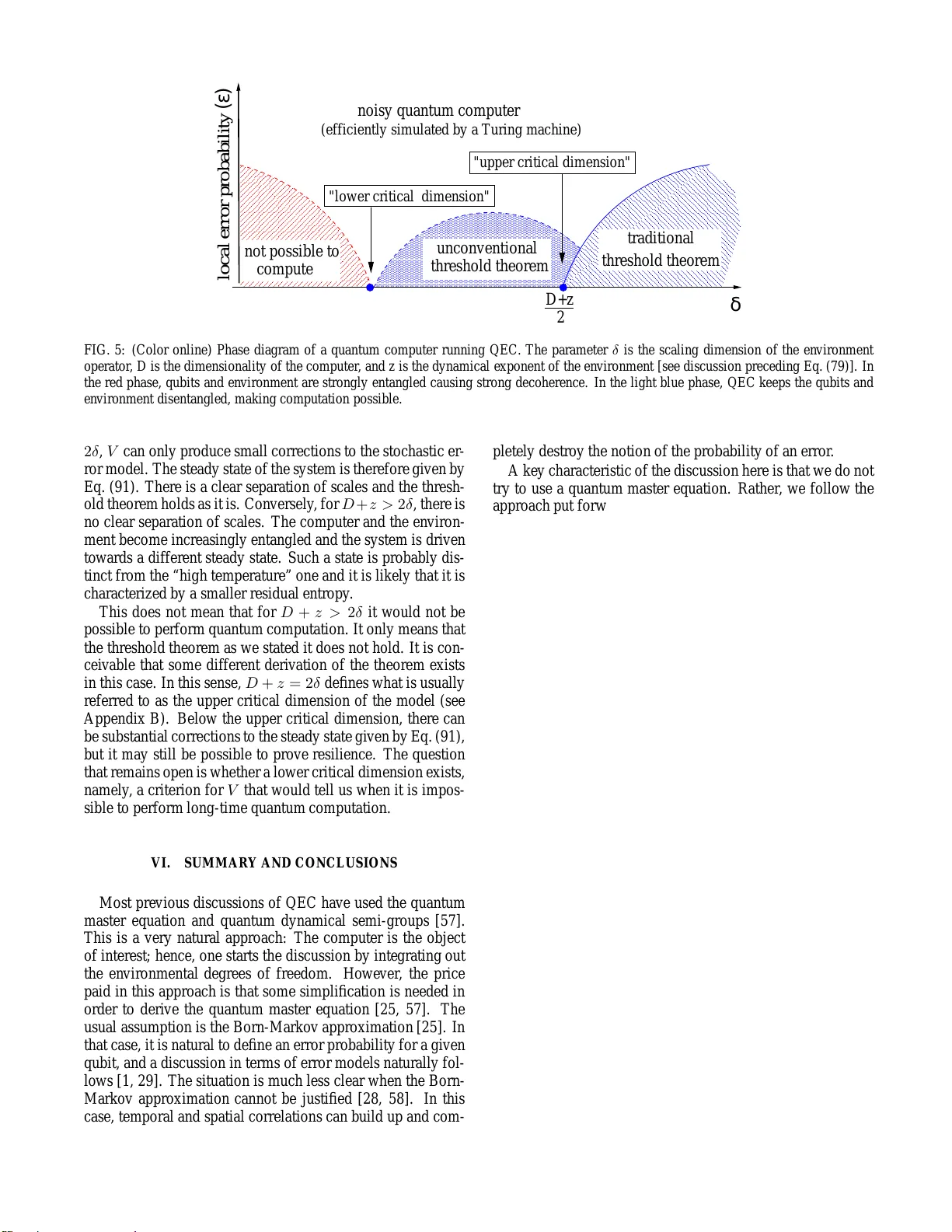
Hamiltonian Formu lation of Quantum Err or Corre ction and Correlated Noise: The Effects Of Syndr ome Extraction in the Long Time L imit E. Novais , 1 Eduard o R. Mucciolo, 2 and Harold U. Baranger 1 1 Department of Physics, Duke University , Box 90305, Durham, North Car olina 27708-0 305, USA 2 Department of Physics, University of Central Florida, Box 162385, Orlando, Florida 32816-2385, USA (Dated: N ov ember 18, 201 8) W e analyze the long time beha vior of a quantum computer running a quantum error correction (QEC) code in the presence of a correlated environ ment. Starting from a Hamiltonian formulation of realistic noise models, and assuming that QEC is indeed possible, we ﬁnd formal expressions f or the probability of a giv en syndrome history and the associated residual decoherence encoded in the reduced density matrix. Systems with non-zero gate times (“long g ates”) are inc luded in our analysis by using an upper bound o n the n oise. In order to introduce the local error probability for a qubit, we assume that propag ation of si gnals through the en vironment is slower than the QEC period (hypercube assumption). This allows an explicit calculation in the case of a generalized spin-boson mo del a nd a quantum frustration model. The k ey result is a dimensional criterion: If the correlations decay suf ﬁciently fast, the system ev olve s towa rd a stochastic error model for which the threshold theorem of fault-tolerant quantum computation has been proven . On the other hand, i f the correlations decay sl o wly , the traditional proof of this threshold theorem does not hold. This dimensional criterion bears many similarities to criteria that occur in the theory of quantum phase transitions. P A CS numbers: 03.67.Lx,03.67.Pp,03.65.Yz,73.21.-b I. INTRODUCTION Quantum comp utation pr ovides a fun damentally new way to process data; as a theory , it is complete and remarkably r ich [1]. Howev er , any real quantum computer is subject to an im- placable ph ysical reality : c ompon ents of a c omputer will al- ways be faulty due to en viro nmental noise. Hen ce, the b uilder of a quantum computer faces the conundru m of ha ving to iso- late the device fr om its surrou ndings an d, simultaneo usly , of needing to act o n it and rea d its output [2]. Many strategies have been de v ised to address this problem [1, 3 , 4, 5, 6, 7], the most general being quantu m error correctio n [1, 8, 9, 10, 11]. Quantum error correction (QEC) should be understood as a perturb ativ e appro ach [12], where one can estimate the proba- bility of having an “error” in the wa ve fun ction of the q uantum computer after a certain time. It is na turally for mulated as a perturb ation expansion in powers o f the coupling between the computer an d the en vironm ent [12]. QEC cannot, in genera l, perfectly corr ect the quan tum evolution, an d the in terferenc e of the am plitudes for th e various processes that occu r implies that quan tum information is always lost to the environment [12]. Howe ver, as we discuss below , QEC can very effec- ti vely slow down this loss. In fact, a ce ntral th eoretical resu lt is the “threshold theorem”: it states that if the error probability is smaller th an a critical value, quan tum comp utation can be sustained indeﬁnitely [13, 14, 15, 16, 17, 1 8, 19, 20, 21]. The word “indeﬁnitely” deserves some clariﬁcation: For the prob- lems that we discuss, it m eans that g iv en a calcu lation and a desired precision, it is alw ays possible to construct a quantum circuit that will p rovide the co rrect result with hig h enough probab ility . QEC h as been largely developed using phenomeno logical “error models”. Rare ly is a connection to a microscopic quan- tum dy namical system found in the literature (see, howe ver, Refs. [22, 23, 24, 25]). In contrast, here we pursu e exactly such a connection : W e discuss the f ormal steps needed to link the theo ry of erro r correctio n with microscopic Hamiltonian models. Furthermo re, because of the perturbative natu re of the method, it is possible to d raw a close parallel between the “threshold theore m” and the theory of qu antum phase tran- sitions. W e ﬁnd that if a c ertain ineq uality ho lds, an err or threshold always exists. When the inequa lity is n ot satisﬁed, either a ne w version of the threshold criterion is required or fault toleran t qu antum co mputation is no t po ssible at all. For the moment, we are not able to distinguish between these two possibilities. Our analysis is based on the fo llowing assump tions. First and foremo st, we assum e that it is possible to p erform the building blocks o f qua ntum erro r correction , nam ely , prepa- ration of states, quantum gates, and m easuremen ts. Seco nd, we con sider th at the en vironm ent is described by a free ﬁeld theory in which therm al ﬂu ctuations can be effecti vely sup- pressed. Finally , the m ain simp lifying assumption o f our d is- cussion is that the qubits are suf ﬁciently separated in space for an entire er ror corr ection proc edure to be p erforme d be- fore correlatio ns betwee n ne arby qu bits develop. Th e pr oba- bility of an error in an individual qubit within a QEC c ycle is, therefor e, indepen dent of a ll o ther qub its. Th is does not im - ply th at ther e are no spatial corr elations; r ather, they d ev elop on long er time scales, while th e err or corr ection pr ocedur e is done faster than a cer tain cha racteristic time. W e emp hasize that th is hyp othesis is no t a limitatio n of the general th eoreti- cal fra mew ork that we describ e, but simply a way to co nnect to the traditional p roofs of the “threshold theorem ” in terms of stochastic error models. The paper is organized as follows. Because of the inter- disciplinary nature of the subject, th is I ntrodu ction continue s with a discussion of two points. First, the dif ﬁculties in taking into a ccount co rrelations in th e en vironm ent are explained in Sec. I A fro m a p erturba ti ve point of view . The n, in Sec. I B, we d iscuss the QEC metho d from a physics v iewpoint and present some results fo r the s tandard stochastic erro r mo del. 2 W e start the body of the paper by developing the r elation be- tween error models and quantu m codes (Sec. II). Th e key issue of QEC in a correlated en v ironmen t is treated in Sec. III. Our m ain r esults d elineating wh en th e perturb ativ e treatment is valid appear in Sec. IV. At the en d of this Section, we provide a brief compar ison between ou r resu lts and those of Ref. 26. Sec. V d iscusses parallels between the threshold the- orem o f QEC and th e theory o f quan tum phase tr ansitions. Finally , in S ec. VI we s ummarize our results and commen t on some open problem s. A. The pro blem of corr elated en vironments In order to set the stage f or the a nalysis in the presenc e of QEC, we ﬁrst look at the p roblem of erro rs crea ted b y a cor related environment in a n un protected sy stem. In the Schr ¨ odinger equation go verning the time e volution of a quan- tum system, th e Hamiltonian H can usually be separated into a single-par ticle term H 0 and a many-p article interaction part V . A f ormal solutio n of this equ ation is given b y th e Dyson series in th e in teraction picture. Solution by iteratio n shows that the time ev o lution operator is U ( t, 0) = T t e − i ~ R t 0 dt ′ V ( t ′ ) , (1) with T t denoting the time order ing o perator and V ( t ) = e i ~ H 0 t V e − i ~ H 0 t . I f V represents the interactio n between th e quantum com puter an d its sur round ings, each in sertion o f V in Eq. (1) corresponds to an “error” in the co mputer e volution. Hence, Eq. ( 1) provides th e natural framework to study the ef- fects of the en viron ment on the state of th e quantum co mputer . It is alw ays po ssible to gi ve an upper boun d to the “er ror probab ility” [27]. The reason is th at Dy son’ s series is abso- lutely c on vergent for ﬁnite times and bou nded o perators (see Append ix A). In sho rt, the b ound ing is do ne by deﬁnin g the “sup” o perator n orm and the ev olution oper ator with at le ast one “error ” (one insertion of V ), E ( t ) = U ( t, 0) − 1 = − i ~ Z t 0 dt ′ V ( t ′ ) U ( t ′ , 0) . (2) The norm of E is related to the p robability of having errors in the computer . Th e calculation is simple and yields ||E ( t ) || ≤ 1 ~ Z t 0 dt ′ || V ( t ′ ) || ≤ Λ t ~ , (3) where we used the tria ngular inequality , the unitar ity of U , an d deﬁned Λ as th e largest eigenv alue of V (with correspo nding eigenv ector Ψ Λ ). One can un derstand th is b ound as simply a restatement of | sin x | ≤ | x | , as follows: E † ( t ) E ( t ) =  2 − U † ( t ) − U ( t )  = 2  1 − T t cos 1 ~ Z t 0 dt ′ V ( t ′ )  (4) so q h Ψ Λ | E † ( t ) E ( t ) | Ψ Λ i = s 2  1 − cos Λ t ~  =     sin Λ t 2 ~     ≤     Λ t 2 ~     . (5) The nor m ||E || has b een very usef ul in pro blems inv o lving non-Ma rkovian noise [26, 27, 28, 29, 30]. Ho wev er , in QEC, an analysis based on the boun d Eq. (3) only makes sense when ||E || ≪ 1 , while we are con cerned with th e long time limit, | Λ t | ≫ 1 , for which this b ound o n the nor m of the error d i- verges. In this case, Dyson’ s series is only asymptotically con- vergent and the “sup” norm i s of no practical use. Hence , it is importan t to express the error probability dif ferently . W e must go back f ull circle a nd reexamine the Dyson series for the time e v olution of a particular state, instead of the worst case scenario explore d by the “sup ” no rm appr oach. Hence- forth, we will be m ainly intere sted in a n inter action Hamilto- nian with the general form V ( t ) = λ Z L 0 d x f ( x , t ) , (6) where λ ≪ 1 is a cou pling co nstant, L is the size of the sys- tem, and f is some fu nction of th e d egrees of freedom of a free theor y wh ose Hamiltonian is H 0 . Because we are inter- ested in corre lated n on-Markovian no ise, w e assume that th e free ﬁelds are s uch that the asymptotic expression for the two- point correlation function is a power law , h Ψ | f ( x 1 , t 1 ) f ( x 2 , t 2 ) | Ψ i ∼ F 1 (∆ x ) 2 δ , 1 (∆ t ) 2 δ/z ! , (7) where ∆ x = | x 1 − x 2 | an d ∆ t = | t 1 − t 2 | [31]. Here, δ is the scaling dimension of f , z is the so-called dyn amical expon ent, and | Ψ i is a ﬁx ed e igenstate of H 0 (which we will usually take to be the ground state of the en vironment) . The motivation for developing a p erturbative expansion of the ev o lution operator (the Dyson series in the interaction pic- ture) is the h ope that a few terms in th e series or a summab le family of them will captur e most of the phy sics. It is then assumed that small couplin g ca n guaran tee fast conver gence. Howe ver, since ||E || is no t necessarily s mall, the nu mber of terms that con tribute substantially to the series can grow faster that th e smallness of consecu tiv e ter ms. In o rder to see that, let us calculate the pro bability of an evolution with errors usin g Eq. (4), h Ψ | E † ( t ) E ( t ) | Ψ i 2 = 1 − h Ψ | T t cos  1 ~ Z t 0 dt ′ V ( t ′ )  | Ψ i . (8) Since we ar e assuming a non-interacting free Hamiltonian, we can use W ick’ s theo rem. It is then straightforward to show that there is at least one term at each order m in the series that contributes “e xtensiv ely” as ∼ λ 2 m ( Lt ) 2 m ( D + z − δ ) . A simple example is gi ven by the serie s of “bubble” d iagrams, where 3 the m th order term is giv en by the contractions Z t 0 dt 1 ... Z t m − 1 0 dt m h V ( t 1 ) V ( t 2 ) i ... h V ( t m − 1 ) V ( t m ) i . (9) Disregarding numerica l prefactors unim portant for our discus- sion, we sum the series as a geometric progr ession to obtain h Ψ | F † ( t ) F ( t ) | Ψ i 2 ∼ λ 2 ( Lt ) 2( D + z − δ ) 1 + λ 2 ( Lt ) 2( D + z − δ ) . (10) Therefo re, for D + z − δ > 0 there is no guara ntee th at the perturb ation series conver ges. Con versely , if D + z − δ < 0 , higher-order terms in the series shou ld be increasing ly less importan t. Thu s, for D + z − δ > 0 th e probability of an e vo- lution with “err ors” tends to on e, whereas for D + z − δ < 0 it will d epend only on the “non- extensi ve” terms in the se- ries. The same analysis can be immediately transpor ted to the study of the ﬁdelity |h Ψ | U ( t ) | Ψ i| , where we see that for a relev ant pertur bation, D + z − δ > 0 , the overlap betwe en the initial state and th e ev olving wav e func tion ten ds to zero (an ortho gonality catastrop he). This sort of “infra red” p rob- lem provides a contact poin t with the th eory o f quantum phase transitions, where the same kind of considerations also appear when calculating th e partition f unction using th e imagina ry time formalism (see Append ix B). In the b ody o f this p aper, our main go al is to tr ansfer these ideas of relev an ce an d i rrelev ance of a perturbation to the e v o- lution of a quantum computer protected by QEC. B. Quantum err or corr ection Quantum er ror cor rection is arguably the most versatile method to protect q uantum infor mation from deco herence [32]. It is a clever use of two features of quan tum mechanics: entanglem ent and (in its tr aditional form ) wa ve p acket reduc- tion due to measurement. T hus, before we start our discu ssion of QEC, it is impor tant to carefu lly d eﬁne what w e mean b y entanglem ent and decoh erence. An entangled state o f two qu antum systems is a state th at cannot b e descr ibed as a direct tensor pro duct of states of in - dividual systems or prob abilistic mix tures of ten sor-product states. As an example, consider tw o physical qubits (hereafter referred to by the subscripts 1 an d 2 ). Each qubit has a Hilb ert space isomor phic to a com plex projecti ve plane of dimension one, CP 1 (see Ap pendix C for d etails). Howe ver , the com- bined Hilbert space is not isomorphic to CP 1 (1) × CP 1 (2) , b ut to the much larger CP 3 . All states in CP 3 outside CP 1 (1) × CP 1 (2) are said to be en tangled. An impor tant subtlety is the implicit notion o f a pr eferred “basis”. Alth ough we can choo se f rom an inﬁnite number of CP 1 × CP 1 subspaces inside the same CP 3 , nature gi ves us a natural choice, namely , CP 1 (1) × CP 1 (2) . In the workin g of a q uantum co mputer, en tanglemen t h as two op posite roles. On the o ne h and, entanglem ent between qubits is the key element in a qu antum co mputation that dis- tinguishes it from its classical co unterpa rt [33]. On th e other hand, when the com puter and the environment b ecome en- tangled, precious quantu m in formatio n is lost. Usually , the latter effect is re ferred to as dec oherenc e. In the literatur e, there are two d ifferent deﬁnitio ns of deco herence. I n a strict sense, decoherence is th e d ecay in time of the coherences (off- diagona l elements of the reduced density matrix), while dissi- pation inv olves the exchan ge of en ergy with the environmen t and chang es in po pulations ( the diag onal term s of the den - sity matrix) . Ho we ver , the word “decohe rence” is also used in a broader sense in volving chang es in bo th diago nal and off-diagonal entr ies of the d ensity matr ix. In this paper we choose the latter use of th e word. The reason is th at from a quantum error correction perspecti ve changes in diagonal and off-diagonal entries are “dual” to each other [1]. There is a simple heuristic explanation for error correction: Usually , no ise is regard ed as a loca l phe nomeno n, thus its damaging effect in th e co mputer should be less p rono unced if the informatio n is delocalize d among se veral qubits. T his is precisely ho w classical error correction codes w ork. A simple example of the latter is a majority vote, where the information of a bit is copied into three physical bits, 0 → 000 an d 1 → 1 11 . If t he probability o f an error in a gi ven qubit is ǫ , the probab il- ity of ha ving tw o independent errors, and consequen tly a total informa tion loss, is ǫ 2 ≪ ǫ . Th us encodin g in creases the lev el of protection of the information . It is temptin g to start explaining QEC fro m this perspec- ti ve. Howev er , the no-clon ing theorem [1] states that it is im - possible to copy an unk nown q uantum state. The altern ativ e approa ch is to u se an entang led state inv olving two or more qubits to store the quantum information . Th is clearly delocal- izes the in formatio n, b ut it is at od ds with the in tuitiv e notion that en tangled states are in g eneral mo re fragile to the effects of the en viro nment (this intuition is driven by the quantum-to- classical transition du e to deco herence, see Ap pendix D fo r a concrete example). Thus, delocalizin g the info rmation u sing entanglem ent does not alone solve the p roblem. It is p ossible to use unitary operations to transfer the entanglement be tween the qubits and the environment to a constant fresh supply of ancilla q ubits [1, 34]. Howe ver , it is more tr aditional in QEC to use the partial measuremen ts of some ancilla qubits to re- duce th e qu antum interf erence with the en vironme nt [1]. Mea- surements here h av e to be u nderstoo d as the projectio n of the state of o ne of the qubits (an an cilla) onto a certain b asis or referenc e state. The outco me of this pro jection is a classical bit (“zero ” or “on e”) and is called a synd rome. T he par tial wa ve packet reduction s c aused by syndro me extraction steer the long-tim e ev olution of the q uantum computer . Recen tly , it has b een shown that the duration of the measu rement is not fundam ental to the QEC pro cedure [35]. In fact, this p rocess can be quite long without jeopard izing the method . A simple example illu strates how QE C works [ 1, 9, 10]. Suppose that we have an er ror model con sisting o f indepen - dent baths fo r each qu bit which can cause on ly phase err ors, and an initial qubit in the state | ψ 0 i = α |↑i + β |↓i that we want to protect. Th e 3-q ubit code p rovides the simplest error correction proced ure for this problem . In Fig. 1 , we deﬁne the encodin g/decodin g methods in a QEC cycle. At th e end of a cycle, the pro bability of m easuring the syndr ome of a phase ﬂip error in one of the three physical qubits is [39] p 1 = 3 ǫ , (11) 4 t 1 t 2 1 2 0 FIG. 1: A 3 qubit quantu m error correction (QE C) code [1, 9, 10, 36, 37 ]. The initial wave function, | ψ 0 i ⊗ ( |↑i + |↓i ) / 2 ⊗ ( |↑i + |↓i ) / 2 , is encoded by two controlled-NO T (CNO T) gates, R CNOT = σ − i σ + i σ x j + σ + i σ − i , into an entangled state | ψ encode i = α ˛ ˛ ¯ ↑ ¸ + β ˛ ˛ ¯ ↓ ¸ with ˛ ˛ ¯ ↑ ¸ = ( |↑↑↑i + |↑↓↓i + |↓↑ ↓i + | ↓↓↑i ) / 2 and ˛ ˛ ¯ ↓ ¸ = ( |↓↓↓i + | ↓↑↑i + |↑↓↑i + |↑↑↓i ) / 2 . A fter some time, it is decoded by a second pair of CNOT gates. An error in | ψ i i s i den- tiﬁed by measuring the v alues of σ x 2 and σ x 3 (rectangle). The QEC cycle end s with the correction of a possible phase-ﬂip (arrow). and the pro bability of the syndro me indicating no err or in the logical qubit is p 0 = 1 − p 1 . (12) The r esidual decoherence that can not be corrected b y th e QEC procedur e is closely related to these probab ilities. I n the case of a cycle in which the syndrome indicates that one error occurre d in any of the p hysical q ubits, dep hasing of the logi- cal qu bit is g i ven by the red uction of th e off-diago nal density matrix element [39], ρ (1) ¯ ↑ ¯ ↓ ≈ αβ ∗ (1 − 2 ǫ ) , (13) while for a cycle with a syn drome indicating no err or , the de- phasing is weaker , ρ (0) ¯ ↑ ¯ ↓ ≈ αβ ∗  1 − 2 ǫ 3  . (14) After N o f these cycles, the prob ability of having m uncorre- lated errors is P m =  N m  p N − m 0 p m 1 , (15) with an associated residual decoher ence of ρ ( m ) ¯ ↑ ¯ ↓ ≈ αβ ∗  1 − 2 ǫ 3  N − m (1 − 2 ǫ ) m . (16) An elegant v isualization of these events is given by a “syn - drome history diagram” of Fig. 2 (see for instance Ref. 28 for a similar d iscussion). An o rdered set of syn dromes labels a particular evolution of th e log ical qub it. From the syndro me history one can ﬁnd the mo st likely evolution an d the asso- ciated residual deco herence. For our 3-qu bit cod e examp le, the most likely ev olution is g i ven by the mean value of m , ¯ m = N p 1 . Thu s, the r esidual decoheren ce of the logical qubit is giv en by ρ ¯ ↑ ¯ ↓ ≈ αβ ∗ e − 6 N ǫ 2 . (17) Therefo re, a s lo ng th e numb er of QEC cycles N ≪ ǫ − 2 , the probab ility of measurin g the correct initial state of the lo gi- cal qu bit is very high . W e can quan tify th e amo unt of infor- mation that is lost b y calculatin g the von Neum ann entro py p 0 p 1 p 0 p 1 p 0 p 1 p 1 p 1 p 0 p 0 t FIG. 2: A syndrome history diagram. Each solid l ine represents the e volution of a logical qubit. At the end of a QEC cycle, a phase ﬂip error is detected or not with probabilities p 1 and p 0 , respectiv ely . A path provides the history of t he logical qubit and is recorded as a sequence of syndrome s. S = − tr ( ρ ln ρ ) : lim N ≪ ǫ − 2 S ≈ 12 N | α | 2 | β | 2 ǫ 2  1 − ln  12 N | α | 2 | β | 2 ǫ 2  (18) lim N ≫ ǫ − 2 S ≈ −| α | 2 ln | α | 2 − | β | 2 ln | β | 2 . (19) Note that the l oss of info rmation can be substantial if the num- ber of cycles is so lar ge that N ≫ ǫ − 2 . If the infor mation need s to b e pro tected for a long p eriod of tim e, we have to modify the p rotection scheme. The mo st straightfor ward approach is to consider a concatenated circuit where each qu bit in Fig. 1 is a logical qu bit itself an d each gate is a logical gate, resulting in an effecti ve reduction of p 1 . Layers an d layers of protection can b e added as needed [1, 29]. A c hief co ncern wh en ap plying this appro ach is whether the steps required in the add ition of mor e qubits and o perations do not actually inc rease the cha nce of erro rs (since they increase the combinatorial factors in the probability distribution). This question is ad dressed by fault-to lerant quantu m compu tation theory [13, 1 5, 16, 17, 1 9, 29], wh ich has as its m ain result the so-called thresh old theo rem: If the “no ise strength” ǫ is smaller than a cer tain critical value, then the intr oduction of an addition al lay er of co ncatenatio n improves the pr otection of the informatio n. A key ingr edient in the deriv ation of the noise thresh old is the assump tion th at a p robabilistic structure similar to the one that we o utlined above exists. Here rests the m ain con - cern of this p aper . There ar e many p hysical situations where an environment can indu ce strong memory effects and spatial correlation s among qubits. Hen ce, it may not be obvious how to d eﬁne the “err or pr obabilities” of a qubit. This hind ers the traditional theory of QEC and th reshold analysis, thus moti- vating a careful study of the d ynamics of q uantum compu ters protected by QEC. 5 II. ERROR MODE LS AND QU ANTUM CODES The syndrome histor y used to describe the logical qubit h is- tory can be converted in to a m ore form al d escription of the computer dynamics. In our discussion, we will assume an en- vironm ent, H 0 , de scribed by a f ree ﬁeld theo ry with a n u ltra- violet cuto ff Λ , a characteristic wav e velocity v , and a d ynami- cal exponent z . Altho ugh simple, a free ﬁeld theory faithfully represents many ph ysically relev ant environments: the elec- tromagn etic ﬁeld, a ph onon ﬁeld, spin waves, a bo sonic bath , or , more gener ally , any two-body d irect in teractions between qubits that was split by a Hubbard- Stratanovich ﬁeld. In addi- tion, we include in the Hamiltonian a ter m to accou nt fo r th e sequence of quantum gates perfo rmed on the qub its, H QC ( t ) . Hence, the total Hamiltonian is H ( t ) = H 0 + H QC ( t ) + V . (20) The inter action ter m will be assume d to have th e form o f a vector coupling between qubits and the en viro nment, V = X x X α = { x,y ,z } λ α 2 f α ( x ) σ α ( x ) , (21) where ~ σ ( x ) are Pauli matrices for the q ubit loc ated at x , λ α are the co upling streng ths, and f α ( x ) are fu nctions of the en- vironm ent operator s [38]. Since [ H 0 , H QC ] = 0 , we a dopt an interaction p icture th at follows n ot on ly th e environment but also the evolution of th e com puter (see Appen dix E). In this rotating frame, the e volution operator is U ( t, 0) = T t e − i ~ R t 0 dt ′ V ( t ′ ) . (22) The in teraction V ( t ) depen ds on the q uantum cod e and its implementatio n. Nevertheless, there are two possible ways to keep the discussion code independen t: (i) In our pre vious work [39, 40], we assumed that quantum gates wer e p erform ed faster than the e n vironmen t respon se time ( which is of o rder th e inv erse of the ultraviolet cutoff frequen cy Λ ). W e call this approxim ation the “fas t gate” lim it. For this case, we h av e the ev olution of th e co mputer between gates giv en by V ( t ) = X x X α = { x,y ,z } λ α 2 f α ( x , t ) σ α ( x ) , (23) with f α ( x , t ) = e i ~ H 0 t f α ( x ) e − i ~ H 0 t . Th en, whe n a g ate is perfor med the actio n o n the qubit is instantaneous an d the sub- sequent e volution is once again gov erned by Eq. (23). (ii) A second p ossibility is to derive an upp er bound on th e effects o f co rrelations. In ord er to do th at, we must ﬁrst dis- cuss how slow gates, which are perform ed over time intervals larger than τ c = 1 / Λ , cha nge Eq . (23). Then, we can deﬁne an effecti ve interaction V eﬀ that takes into accoun t the slowness of the gates and serves as an u pper boun d to the exact ( and code-d ependen t) V . Clearly , the real experimental situatio n rests between the two limits (i) and (ii). Before we begin a detailed d escription of how to han dle case ( ii), let us note that here the term inology “fast” and “slow” gates fo llows the QEC literature: Fast (slow) gates have a d uration m uch sho rter (long er) than τ c . Howev er , as will become clear later , the rele vant time scale that appears in the study of correlation effects is the period or duration of the error corr ection cycle, ∆ . Th us, in that co ntext, short (“fast”) or long (“slow”) dynam ical effects will b e n aturally d eﬁned with respect to ∆ , and not to τ c . Any quantum computer code is just a rotation in the Hilbert space of the qubits an d can be described a s a trajectory on CP 2 N − 1 , where N is the total num ber of q ubits. In the Schr ¨ odinger p icture, the ev olution is g iv en by the natu- ral ac tion on S 4 N − 1 by S U (2 N ) . The most gene ral fault- tolerant qu antum circuit is therefo re d eﬁned by th e Hamilto- nian H QC ( t ) = P b j ( t ) e j , where { e j } are the g enerator s of the Lie a lgebra of S U (2 N ) . The e volution operator ass ociated with this Hamiltonian satisﬁes the integral equation W ( t, 0) = 1 − i ~ Z t 0 dt ′ H QC ( t ′ ) W ( t ′ , 0) = T t e − i ~ R t 0 dt ′ H QC ( t ′ ) , (24) such that the comp uter state vector at time t is given b y | ψ ( t ) i = W ( t, 0) | ψ (0) i , wh ere | ψ (0) i represents the initial state of the co mputer . There fore, in th e interaction picture, the interaction operato r is giv en by V ( t ) = W † ( t ) e i ~ H 0 t V e − i ~ H 0 t W ( t ) (25) = X x X α = { x,y ,z } λ α 2 h e i ~ H 0 t f α ( x ) e − i ~ H 0 t i × W † ( t ) σ α ( x ) W ( t ) = X x X α = { x,y ,z } λ α 2 f α ( x , t ) W † ( t ) σ α ( x ) W ( t ) . (26) Since W ( t ) is a S U (2 N ) matrix, then G α ( x , t ) = W † ( t ) σ α ( x ) W ( t ) (27) is another matrix of S U (2 N ) , and we can write V ( t ) = X x X α = { x,y ,z } λ α 2 f α ( x , t ) G α ( x , t ) . (28) Although the expression in Eq. (28) is general, it is not very instructive. Fur thermor e, it is very und esirable fr om an er- ror cor rection standpoint: since G ( t ) is an a rbitrary matrix o f S U (2 N ) , the V ( t ) in E q. ( 28) in prin ciple gene rates a h ighly complex correlated err or that is nevertheless ﬁrst ord er in the coupling to the e n vironmen t. The p roblem with the de riv a- tion of Eq. (2 8) is th at it is too gen eral since we a ssumed that arbitrary r otations are p erforme d at each sin gle step. How- ev er , o ne o f the corn erstones of qu antum com putation is that such general rotations can be approxima tely d ecompo sed into a ser ies o f elemen tary gates [1]. Hen ce, our strategy will be to specialize the calcula tion to these elemen tary gates and as- sume that gene ral rotation s can be implemen ted by a ﬁnite series of such gates which are well resolved in time. 6 A. Single-qubit operations When only single-qub it operations are perfo rmed, we have H QC ( t ) = X x X α = { x,y ,z } b α ( x , t ) σ α ( x ) . (29) In this case, W ( t ) is the pro duct of S U (2) matrices acting in each qubit’ s Hilbert space. Thus, G α ( x , t ) simpliﬁes to G α 1 ( x , t ) =  ρ 1 e − iφ − ρ 2 e iϕ ρ 2 e − iϕ ρ 1 e iφ  σ α ( x )  ρ 1 e iφ ρ 2 e iϕ − ρ 2 e − iϕ ρ 1 e − iφ  , (30) where ρ 2 1 + ρ 2 2 = 1 and { ρ 1 , ρ 2 , φ, ϕ } are f unctions o f x and t . The single- qubit rotations yield an expression of the form G α 1 ( x , t ) = X β = { 1 ,x, y ,z } g αβ ( x , t ) σ β ( x ) (31) for some g αβ ( x , t ) . By deco mposing th e oper ators f α and function s g αβ into their Fourier c ompon ents, we ca n g iv e a more formal meaning to “fast” and “slo w” gates, f α ( x , t ) g αβ ( x , t ) = X | ω 1 | < Λ ,ω 2 e i ( ω 1 + ω 2 ) t f α ( x , ω 1 ) g αβ ( x , ω 2 ) . (32) Hence, if we d eﬁne ν = ω 1 + ω 2 , we can rewrite the pertur- bation as V = X β ( X ν e iν t " X ω 2 X α f α ( ν − ω 2 ) g αβ ( ω 2 ) #) σ β . (33) In the limit of fast gates, | ω 2 | > Λ , f an d g are not conv o lved, since they have distinct frequen cy do mains. Therefor e, the noise o perators f α are unaltere d b y the r otation. However , if g has a signiﬁcant weight at freq uencies smaller than Λ (slo w gates), one must conv olve f with g , yielding a sub stantially different noise operator . B. T wo-qubit operations The general Hamiltonian for two-qubit gates is of the form H QC ( t ) = X x , y X α,β = { x,y ,z } J αβ ( x , y , t ) σ α ( x ) σ β ( y ) . (34) Howe ver, one can also generate a full set o f gates u sing instead a single type of interaction, H QC ( t ) = X x , y J ( x , y , t ) σ a ( x ) σ b ( y ) (35) where a and b a re ﬁxed fo r each g ate ( x , y ) . I n order to see that th is is sufﬁcient we c an f or in stance set a = b = z . This generates the liq uid N MR Hamiltonian [4 1], wher e the Ising interaction, Eq. (35), and single qubit rotations can be used to generate a contro l σ z gate. W e keep a and b ar bitrary . Howe ver, for th e sake of sim- plicity , we assume that only op erations between disjoint pairs are allowed; that is, if J ( x , y 1 , t ) 6 = 0 , th en J ( x , y 2 , t ) = 0 for all y 2 6 = y 1 . It is then straightforward to write down W ( t ) in a co mpact fo rm: The time- orderin g [Eq. (2 4)] is auto mati- cally taken care of by the sequen ce of gates, wh ile for a gate in volving qubits x a nd y the contribution to W ( t ) is W ( x , y , t ) = cos [ θ ( x , y , t )] (36) + i sin [ θ ( x , y , t )] σ a ( x ) σ b ( y ) , where θ ( x , y , t ) = R t 0 dt ′ J ( x , y , t ′ ) . He nce, a two-qubit rota- tion yields G α 2 ( x , t ) = sin [2 θ ( x , y , t )] ǫ aαγ σ γ ( x ) σ b ( y ) + co s [2 θ ( x , y , t )] (1 − δ a,α ) σ α ( x ) + δ a,α σ α ( x ) , (37) where ǫ aαγ is the usual antisymmetric tensor . The ﬁrst term on the r .h.s. of Eq. (37) tells us that the 2-qubit gate can propagate the error from the qubit at x to the qubit at position y . Howe ver , it also tells u s that it is po ssible to choose a particular gate whe re this prop agation does no t happen (by choosing a = α , f or instance ). Un fortuna tely , propag ating errors in th e qu antum circ uit is in general unav oidable (since the o nly g ate that commu tes with all Pauli o perators is the identity). The second and third terms on the r .h .s. of Eq. (3 7) are much less dramatic. Th ey simply describe a local noise that is not propa gated by the gate. C. Upper -bounds f or the ev olution In Eqs. (31) an d (37), we showed that o ne- and two-qub it gates can intro duce what is seemingly a very comp licated noise structur e. The expression s depend on how the g ates are implemented , thus hiding a gener al assessment. W e can ad- vance the discussion by r ecalling that W is always an un itary matrix. Hence, the coefﬁcients in E qs.(31) and (37) have mod- ulus equal or smaller than u nity . A suitab le upper boun d on the effects of slow gates is th en provided by setting all these coefﬁcients eq ual to one. Thus, the op erators expressed in Eqs. (3 1) and (37) gain the upper bounds ˜ G α 1 ( x ) = X β = { x,y , z } σ β ( x ) , (38) ˜ G α 2 ( x ) = σ α ( x ) + ǫ aαγ σ γ ( x ) σ b ( y ) . (39) ˜ G α 2 still look s trou blesome, since it tells u s that an error in qub it x is pro pagated to y . Howe ver, th is is not a prob - lem of the ﬁnite gate time o peration , since an instantan eous and perfect gate will also propagate the error in a similar fash- ion. In order to obtain an upp er bo und for the effects intro- duced by the two-q ubit gates, we pre cisely f ollow this fact. W e consider that all the qubit compo nents are exposed to all the n oise cha nnels all the time. Th us, we replace E q. ( 39) b y G α 2 ( x ) = P β = { x,y , z } σ β ( x ) and assume that two-qubit gates 7 are per formed in stantaneously . In summ ary , we red uce the problem of ﬁnite time op eration of the two-qub it gate to the problem of a noisier qubit environment and propagating er rors in the quantum code by perfect gates. Now we can rely on the theory o f fault-tolerance [ 1, 29], and simply assume that the error propag ation is handled by the quantum code. The ﬁnal conclusion is that an upper bound estimate on the effects o f slow g ates is obtained by the inte raction Hamilto- nian V eﬀ ( t ) = X x X α = { x,y ,z } λ 2 f eﬀ ( x , t ) σ α ( x , t ) , (40) where f eﬀ ( x , t ) = 1 λ 2   X β = { x,y , z } λ β f β ( x , t )   (41) and λ = q P β = { x,y , z } λ 2 β is the n ew coup ling parame ter . Although th is is a br utal app roximatio n, it will be sufﬁcient for our discu ssion. As we will argue later , for the pu rpose of determin ing the effect of long -wa velength co rrelations on the threshold the orem, th e only relev ant aspect of the f α is their scalin g d imension. Since dim f eﬀ is in gen eral eq ual to min (dim f α ) , it is sufﬁcient to use Eq. (40) as the worst case scenario. Thus, in b oth limiting ca ses, fast an d slow gates, we ar- rive at the same fu nctional form fo r the effective interaction. Hence, both cases can be handled simultaneously , and we pr o- ceed to the analysis of QEC in the p resence of this interaction. In order to simplify th e notation, we her eafter drop the sub - script “eff ” from the slow-gate operators. III. Q U ANTUM ERROR CORRECTION IN CORRELA TED ENVIRONMENTS A QEC code is deﬁned as the com bination of enco ding, decodin g, and recovery op erations. Since we were able to make our an alysis co de indepe ndent, the unitary c ompon ent of the QEC pro tocol is descr ibed by U (∆ , 0) , Eq. ( 22), with the appropriate V ( t ) discussed in Sec. II. The ﬁnal ingredient in standard QEC is just the syndrom e e xtraction P , which is a projective measurement. In Ref . 39 it was dem onstrated h ow to deﬁn e P and its ef- fects on U for stabilizer error correction codes. I t is important to re mark tha t an er ror whic h keeps th e com puter in the logi- cal Hilbert space can nev er be corrected by QEC. This is sim- ply a statement that for the general assumptions we make, the problem of protecting quantum information nev er satisﬁes the second c riterion of Lafﬂame-Knill [ 12] f or pe rfect QEC. In simple terms, the criteria states that all allo wed errors must al- ways take the logical one and logical zero to orthogon al states [Eq. (20) of Ref. 12]. By co nstruction, these error s ar e hig h- order events in th e couplin g with the en vironmen t. Neverthe- less, as we alread y know (I A), this fact per se is not enou gh to ensur e that su ch err ors will n ot be relevant at lon g times. One of our goals is to ﬁnd out when it is appr opriate to safely neglect such uncorrectab le error s in the presence of correlated en vironme nts. In hind sight, it is not hard to understand the b eneﬁts of QEC. Thus, for the sake of readability , we present ﬁrst a qual- itati ve argument that captures the overall discussion. As we deﬁn ed in the introduction, there are two q uanti- ties that we are interested in calcu lating: (i) th e p robab ility of a gi ven e volution, and (ii) t he reduced density matrix of the computer . Both quantities are written as a doub le series in the coupling with the environment. On the one hand , the initial ket of computer and the en viro nment, | Ψ i , e volves in the time interval [0 , t ] b y the time ordere d series U ( t ) . On the oth er hand, the b ra h Ψ | ev olves in time with th e anti-time-or dered series U † . It is only a subset of each serie s that enters in the ev alu ation of either the probability or the reduced density ma- trix, because of the measuremen ts present in the tr aditional formu lation of QE C. H ence, it is u sually a non -trivial task to calculate the necessary expectation v alu es. Because w e ar e d ealing with a doub le series, it is natu ral to use a for malism analog ous to a time -loop expan sion [ 42]. There are six (in terrelated) Green fu nctions in such an ex- pansion: Th e u sual a dvanced and re tarded function s for the time-orde red series; the advanced and re tarded fu nctions for the an ti-time-ord ered series; an d the lesser and grea ter fun c- tions, which contract a term from the time-orde red series with another one from the an ti-time-ord ered series. This formal- ism is often re ferred to as th e Schwinge r-K eld ysh ap proach [43, 44]. It is usua lly r epresented graphica lly by a do uble contour in time ( see Fig. 3). T he upper le g stands for the time- ordered evolution f or the time interval [0 , t ] , while th e lower leg stand s for th e anti-tim e-order ed ev olution in th e reversed interval [ t, 0] . Let u s for the m oment ass ume that a short-time expan sion is t t t 1 3 4 t t 2 (a) 1 2 t t t t 3 4 t (b) t 1 t 2 t t 1 2 t (c) t 1 t 1 t t 2 t 2 (d) FIG. 3: Graphical representation of a few f ourth-order terms i n a “time-loop” expans ion for either the probability of a given e v olution or the reduced density matrix (spatial dimensions are suppressed for clarity). Points o f interaction with the bath (circles) are connec ted by propagation of the en vironmental modes (wiggly lines). In the top diagrams, the time integrals are unconstrained , as would be the case for unitary ev olution. In the bottom diagrams, the detection of an error by a QEC protocol forces the interactions with the bath to occur at t he same times on both the forward and backward l egs in order that U and U † correspond to the same syndrome. This additional constraint introduced by QEC is crucial in the long-time beha vior . 8 valid and focus on a single q ubit. The n, the e volution op erator for that particular qubit within a QEC cycle is gi ven by U 1 (∆ , 0) ≈ 1 − i ~ Z ∆ 0 dt X α = { x,y ,z } λ α 2 f α ( x , t ) σ α ( x , t ) − 1 ~ 2 Z ∆ 0 dt Z t 0 dt ′ X α = { x,y ,z } λ α λ β 4 f α ( x , t ) f β ( x , t ′ ) σ α ( x , t ) σ β ( x , t ′ ) + O ( λ 3 ) . (42) In Fig. 3 we represent graphically a fe w terms o f order λ 4 . All of these terms are the product of a second-or der term from U 1 and a seco nd-ord er term from U † 1 [see Eq . (42)]. Hence, th ey correspo nd to two “errors” in the qub it ev o lution an d inv olve the expectation v a lue h Ψ | f † α ( x , t ) f † β ( x , t ′ ) f α ( x , t ′′ ) f β ( x , t ′′′ ) | Ψ i . (43) Using W ick ’ s theorem, we can immediately write (43) as a produ ct of the non-interacting Green functions. Each possible set of contractio ns leads to the different “diagrams” in F ig. 3. W e usually do not k now when an “err or” occur s; hence, each Green fu nction is acc ompanied in the series by a d ouble integral in time. This is precisely the case in an unpro tected computer ’ s ev olution or inside a QEC cycle [see Fig s.3 ( a) a nd (b)]. Howe ver , a dramatic cha nge ha ppens in a Green f unction between ter ms fo r d ifferent cycles. When the syn drome shows that a particular error occurr ed in a certain QEC cycle, we can re-write Eq. (4 3) to reﬂect this knowledge: h Ψ | f † α ( x , t ) f † β ( x , t ′ ) f α ( x , t + δ t ) f β ( x , t ′ + δ t ′ ) | Ψ i , (44 ) where δ t and δ t ′ are time variables with rang e smaller than the QEC period. After integrating the “h igh freq uency” part (the δ t and δ t ′ variables), we end up reducing Eq. (44) to h Ψ | f † α ( x , t ) f † β ( x , t ′ ) f α ( x , t ) f β ( x , t ′ ) | Ψ i (45) with t and t ′ representin g a coarse-grained time scale of order the QEC perio d [see Figs. 3 (c) a nd (d)]. Th erefore , although we are consider ing term s o f the sam e order in λ , the nu mber of “time integrals” in the co arse-grain ed scale (low fre quen- cies) is half that in th e or iginal micro scopic calcu lation (hig h frequen cies). The simple dim ensional analy sis o f Sec. I A tells us now that QEC ha s ch anged the criteria for th e stability of the p er- turbation series at long times. As we dem onstrate now , it is less stringent than the naive expectation. A. Quantum ev olution steered by QEC It is reasonab le to assume that at the beginning of the com- putation th e c omputer ’ s state vecto r , ψ 0 , and the en viron- ment’ s, ϕ 0 , are not entang led, | Ψ ( t = 0) i = | ψ 0 i ⊗ | ϕ 0 i . (46) In a r ealistic situation, ψ 0 would h av e some in itialization error and be entang led with the environment to some d egree (b oth of which would yield er rors in ψ ). However , her e we neglect these effects in order to keep the discussion focused. Just as in the case of the 3-qub it code, by the end of a QEC cycle the compu ter will have e v olved accordin g to the unitary operator U (∆ , 0) . Then , the sy ndrom e is extracte d a nd the computer wa ve fun ction is projected, P m U (∆ , 0) | Ψ (0) i , (47) where m correspo nds to a particular sy ndrom e, with P m P m = I an d P 2 m = P m . In the case of many logical qubits ev o lving together, then m denotes the set of all the syndrom es extracted at time ∆ . The last step in the co de is the appro - priate recovery o peration, R m , dep ending o n the syndrom e outcome, | Ψ (∆) i = R m (∆ + δ, ∆) P m U (∆ , 0) | Ψ (0) i . (48) Since in a fault-tolerant erro r correctio n schem e the infor- mation is never dec oded (in contrast to the 3-qu bit cod e dis- cussed ab ove), the q uantum info rmation always r emains pro - tected. Th erefore , we can deal with our two limiting cases (slow- and fast-gates) in two d ifferent ways. In the case o f a slow-gate recovery , we f ormally include it a s the initial step of the n ext QEC perio d. Conversely , in the case o f fast g ates, we assume that the recovery is perform ed ﬂawless ly in a very short time scale after th e pro jection. For the sake of clarity , we cho ose the latter b elow . W e emphasize that this d oes not restrict ou r discussion, since it is kn own that the time o f re- covery is irrelev ant to the er ror c orrection . In fact, it can b e postpone d all the way to the end of the calculation [35]. B. Probability of a syndr ome history and the loss of informa tion The ﬁrst quantity to discuss is the pro bability of measuring a particular syndrome at the end of the ﬁrst QEC step, P m = h Ψ(0) | U † (∆ , 0) P m U (∆ , 0) | Ψ(0) i . (49) The correspo nding reduced density matrix is 9 ρ m ~ r ,~ s (∆) = tr ε  h ~ r | P m U (∆ , 0) | Ψ(0) i h Ψ(0) | U † (∆ , 0) P m | ~ s i  h Ψ(0) | U † (∆ , 0) P m U (∆ , 0) | Ψ(0) i = h ϕ 0 |  h ψ 0 | U † (∆ , 0) P m | ~ s i h ~ r | P m U (∆ , 0) | ψ 0 i  | ϕ 0 i h ϕ 0 | h ψ 0 | U † (∆ , 0) P m U (∆ , 0) | ψ 0 i | ϕ 0 i , (50) where ~ r and ~ s denote states in the computer Hilbert space and tr ε is the trace ov er the en viro nment Hilbert space. It is possi- ble to quantify how much information w as leaked to the en vi- ronmen t by calculating the von Neumann entropy S (∆) = − tr c [ ρ m (∆) ln | ρ m (∆) | ] , (5 1) where tr c is the trace over the computer Hilbert space. In Eqs. (49) and (5 0), o ne clear ly sees the imp ortant role played by the pro jection oper ators in the qu antum ev olution steered by QEC. The carefu l constru ction o f the encod ed states combine d with the measu rement (syn dromes) red uces the qua ntum interfe rence b etween different history p aths o f the computer . By partially collapsing the wave f unction of th e computer, this traditional form of QEC reduces decoheren ce. Equation s (49) and (50) deﬁne the local c ompon ents of the noise. When spatial co rrelation between qubits can be ig- nored, they are related to the stochastic probabilities and den- sity matrix discussed in Sec. I B [see Eqs. (15) and (1 6)]. The generalization to a sequence of QEC cycles is straight- forward [39], Υ w = υ w N  N ∆ , ( N − 1 )∆  ...υ w 1 (∆ , 0) , (52) where w is the par ticular history of syndro mes for all the qubits and υ w j  j ∆ , ( j − 1)∆  = R w j  j (∆ + δ ) , j ∆  P w j U  j ∆ , ( j − 1)∆  , (53) is the QEC ev olution af ter e ach cycle. E ach history comes with the associated prob ability P ( Υ w ) = h ϕ 0 | h ψ 0 | Υ † w Υ w | ψ 0 i | ϕ 0 i . (54 ) Finally , there is always some residu al decoheren ce which can be found from the reduced density matrix ρ ~ r,~ s (Υ w ) = h ϕ 0 |  h ψ 0 | Υ † w | ~ s i h ~ r | Υ w | ψ 0 i  | ϕ 0 i h ϕ 0 | h ψ 0 | Υ † w Υ w | ψ 0 i | ϕ 0 i , (55) with ~ r and ~ s bein g elem ents of the logical subsp ace. This in turn yields the entropy S (Υ w ) = − tr c  ρ (Υ w ) ln | ρ (Υ w ) |  . (56) In th e fo llowing, we will sh ow for Eqs. (54) an d (5 5) how to separate the effect of co rrelations betwe en different QEC cycles from the co ntributions du e to the lo cal comp onent of the noise, as deﬁned by Eqs. ( 49) and (50). IV . PER TURBA TION THEOR Y AND THE HYPERCUBE ASSUMPT ION There is one additio nal issue that we must deal with be fore we can move for ward. In prin ciple, even the ﬁrst ord er term in Eq. (42) is already be yond t he QEC approach that has been outlined so far . Th e reason is th at when calcu lating P o r ρ we gen erate pair contr actions o f th e typ e h f α ( x , t ) f α ( y , t ′ ) i . Therefo re, the prob ability of ﬁn ding an err or a t a giv en qub it is condition al on wh at ha ppens with all other qub its. This automatically hin ders the simple probab ilistic interp retation of QEC that we used in Sec. I B. The fact that we do no t want to deal with such cond itional probab ilities leads us to the single most im portant s implifying hypoth esis of o ur work: W e assum e that the q ubits are sepa- rated by a minimum distance ξ = ( v ∆) 1 /z , (57) where v is the excitation velocity and z is the dyn amical ex- ponen t o f the theor y de scribing the environment. Hence , for all x 6 = y an d | t − t ′ | < ∆ , we h av e h f α ( x , t ) f α ( y , t ′ ) i ≈ 0 . It is then possible to assign a p robab ility f or the short-time ev o lution of each qubit independe ntly of all others. T o further organize the analysis we order the qubits in a D - dimensiona l array that deﬁnes hypercube s of volume ∆ × ξ D (see Fig. 4). I n summary , for times smaller than ∆ , each qubit has a dynam ics in depend ent f rom the o ther qub its, hence r e- sembling a qua ntum imp urity p roblem. Ho wev er , f or time scales larger th an ∆ , spatial co rrelations among them are present, thus making the problem similar to a spin lattice. Ideally , we w ould lik e to decompose the ev o lution operator in inter- and intra-hypercu be c ompon ents, U (∆ , 0) = U < (∆ , 0) U > (∆ , 0) , (58) where < labels frequencies smaller than ∆ − 1 and > frequen- cies in the interval  ∆ − 1 , Λ  . Whenever this is possible, we can integrate the intra-hypercu be part in order to deﬁne a “lo- cal” ev olution and, co nsequently , a lo cal error prob ability . ξ ∆ FIG. 4: T wo neighboring hypercubes in space-time, each one con- taining a qubit. 10 There are simple noise models where this can be done exactly [39], however , in g eneral, this sep aration is on ly possible in a per turbative e xpansion. Keeping just a few terms in p ertur- bation th eory is no t always adequ ate, an d we must tr y to ﬁnd ways to improve it. A. Perturbation theory impr ov ed by RG Our ob jectiv e in th is section is to deﬁne an effectiv e evo- lution oper ator that can reasonab ly describe the evolution of the qubit within each h ypercu be. All terms con sistent with the same syn drome and having the same lead ing lon g-time pr op- erties sho uld be includ ed. W ithin a hy percub e, the environ- ment indu ces interaction of a qu bit only with itself; com mu- nication betwe en qubits at lon ger tim es is treated in the n ext section. W e u se the r enormaliza tion gro up (RG) [45] to sum th e most relevant families o f terms in the p erturbatio n series. In order to impr ove the lowest orde r terms in the pertur bation theory thr ough RG, we ne ed to introduce the next higher-order terms in the pertu rbation series. Howe ver , as we discussed previously , we ar e no t intere sted in th e fu ll un itary ev o lution, but rathe r the projected terms o btained af ter th e extraction of the synd rome. T herefor e, in o rder to app ly RG to the ﬁrst- order term, we need to consider υ α ( x 1 , λ α ) ≈ − i 2 ~ λ α Z ∆ 0 dt f α ( x 1 , t ) − 1 8 ~ 2 | ǫ αβ γ | λ β λ γ σ α (∆) T t Z ∆ 0 dt 1 dt 2 f β ( x 1 , t 1 ) f γ ( x 1 , t 2 ) σ β ( t 1 ) σ γ ( t 2 ) + i 48 ~ 3 X β λ α λ 2 β σ α (∆) T t Z ∆ 0 dt 1 dt 2 dt 3 f α ( x 1 , t 1 ) f β ( x 1 , t 2 ) f β ( x 1 , t 3 ) σ α ( t 1 ) σ β ( t 2 ) σ β ( t 3 ) , (5 9) where ǫ αβ γ is the antisymmetr ic ten sor [46]. Ther e is only one spatial ind ex in (59) b ecause of the h ypercu be assump- tion: we have includ ed on ly terms in which contrac tion of the f ’ s yields a non -zero v alue, as these will co ntribute to the effecti ve s hort time ev olution. At lon g times, conn ections be- tween the qubits are, of course, essential, and this is treated in the next section. The RG is naturally implemented in the case of ohmic bath s (which leads to logar ithmic sing ularities). Howe ver, suitable generalizatio ns can be deﬁned by dimension al regular ization or by summ ing series in th e expansion. Thus, in general, it is possible to write the following beta function for υ α x 1 : dλ α dℓ = g β γ ( ℓ ) λ β λ γ + X β h αβ ( ℓ ) λ α λ 2 β , (60) where g an d h are func tions speciﬁc to a particular environ- ment, ℓ = Λ / Λ ′ , an d Λ ′ is the red uced (i.e. rescaled ) cuto ff frequen cy . By integrating the beta function from the bare cut- off, Λ , to ∆ − 1 , we are summing the most rele v ant comp onents of th e noise inside a hype rcube. If the reno rmalized value of the run ning cou pling at frequen cy ∆ − 1 , λ ∗ , is still a small number, then it is a good approximatio n to consider υ α ( x 1 , λ ∗ α ) ≈ − iλ ∗ α 2 ~ Z ∆ 0 dt f α ( x 1 , t ) (61) as the e volution opera tor of the qubit at p osition x 1 which was diagnosed with an error α by the QEC procedur e. W e illustrate the renorma lization group procedur e with two simple examp les o f ohmic b aths: (i) marginally relev ant an d (ii) marginally irrele v ant couplings. 1. The k-c hannel K ondo pr oblem The ﬁr st examp le is a qu bit expo sed to a bosonic b ath th at is modeled by a S U (2) k Kac-Mood y algebra – the bosonized Hamiltonian of a k -channel K on do problem . Here we clo sely follow the work o f Afﬂeck and Lu dwig (see append ix B of Ref. 47). W e deﬁne chiral boson ic currents : ~ J L : obeying the operator product expansion (OPE) : J a L ( t ) : : J b L ( t ′ ) : → f abc : J c L ( t ) : v ( t − t ′ ) − k δ ab 2 v 2 ( t − t ′ ) 2 , (62 ) where f abc are the gro up structu re co nstants and v is the ve- locity of excitations. In the in teraction pictur e, the qu bit cou- ples to the curren ts by the usua l K ondo interaction , yielding an ev o lution operator (or, equiv alen tly , a scattering matrix) of the form U = T t e − iλ v 2 ~ R ∞ −∞ dt : ~ J L ( t ) : · ~ σ . (63) Follo wing ou r g eneral discussion, we expand the ev o lution operator to lowest order in the coupling, U ≈ 1 − iλ v 2 ~ Z ∞ −∞ dt : ~ J L ( t ) : · ~ σ −  λ v 2 ~  2 X a,b Z ∞ −∞ dt Z t −∞ dt ′ : J a L ( t ) : : J b L ( t ′ ) : σ a σ b 11 + i  λ v 2 ~  3 X a,b,c Z ∞ −∞ dt Z t −∞ dt ′ Z t ′ −∞ dt ′′ : J a L ( t ) : : J b L ( t ′ ) : : J c L ( t ′′ ) : σ a σ b σ c . (64) Due to the QEC ev olution, only some of these terms are kept after the syn drome is extracted [see Eq . (5 9)]. For clarity , let u s assume that we know f rom the syndro me that a phase ﬂip has occurred . Hen ce, we must truncate the e volution operator to reﬂect this fact and apply the recovery operation (in this case multiply by σ z ), yielding v z ≈ − iλ v 2 ~ Z ∞ −∞ dt : J z L ( t ) : − i  λ v 2 ~  2 Z ∞ −∞ dt Z t −∞ dt ′ [: J x L ( t ) : : J y L ( t ′ ) : − : J y L ( t ) : : J x L ( t ′ ) :] + i  λ v 2 ~  3 X a Z ∞ −∞ dt Z t −∞ dt ′ Z t ′ −∞ dt ′′ [: J a L ( t ) : : J a L ( t ′ ) : : J z L ( t ′′ ) : + : J z L ( t ) : : J a L ( t ′ ) : : J a L ( t ′′ ) : − : J a L ( t ) : : J z L ( t ′ ) : : J a L ( t ′′ ) :] . (65) Now , we in tegrate over a sma ll frequ ency sh ell [Λ − δ Λ , Λ] and inv oke the OPE. The r esult is a renorm alization o f the coupling λ b y an inﬁnitesimal composed of quadratic and cu- bic terms, dλ dℓ = λ 2 − k 2 λ 3 . (66) The resulting runn ing cou pling λ ( ℓ ) can be u sed to improve the resu lts of our bare pertu rbation theor y . For that purp ose, we integrate the beta function from the bare cutoff until ∆ − 1 . For the case of a small number of channels, we obtain a renor- malized couplin g of the form λ ∗ ≈ λ 1 − λ ln | Λ∆ | . ( 67) Although the RG ﬂow go es toward the strong co upling limit, we do n ot integrate the be ta fun ction all the way to zero fre- quency . Thus, if th e ren ormalized couplin g λ ∗ is still a small parameter, it replaces λ leading to the ﬁrst-order renormalized ev o lution v z ≈ − iλ ∗ v 2 ~ Z ∞ −∞ dt : J z L ( t ) : σ z . (68) 2. Quan tum frustrated system Correlations are not necessarily malignan t to the com- puter’ s beh avior . Th is is illustrated by ou r secon d example: a qua ntum fr ustrated en vironmen t [48, 4 9, 50]. Consider the case of th ree in depend ent Abelian ohm ic ba ths coupled as in Eq. (63), but with the OP E : J a L ( t ) : : J b L ( t ′ ) : → − δ ab 2 v 2 ( t − t ′ ) 2 . ( 69) Follo wing pr ecisely th e same methodolo gy of th e pre vious ex- ample, we obtain the beta functio n dλ dℓ = − 1 2 λ 3 , (70) which leads to the renormalized coupling λ ∗ ≈ λ p 1 + 2 λ 2 ln | Λ∆ | . ( 71) A q uantum fru strated system has th e rem arkable pr operty of asymptotic fre edom. Hence, even very large b are co uplings ﬂow towards a pertur bativ e regime. The physical re ason b e- hind this is the lack o f a p ointer basis [5 1], thus e ffecti vely decoup ling the qubit fro m its surroun dings [ 49]. This phe- nomena can a lso be u nderstoo d as self-inﬂicted π -pu lse de- coupling working at the cutoff frequency Λ [7, 52]. If the thr ee cou pling constan ts have different bar e values, then the ﬂow stop s at some ﬁnite freq uency since two of the coupling s w ill ﬂow to zer o be fore the third. In other words, there will be a pointer basis. In a quantum computer protected by QEC, howe ver , we are effectively stopp ing the ﬂow at a ﬁnite freq uency . Hence, the effect describ ed in the previous paragra ph is relev ant e ven for large anisotropic couplings. B. Probability of a faulty p ath Now th at we have o btained a rea sonable app roxima tion to the ev olution op erator at each QEC step , we can turn to th e problem of evaluating how much pr otection QEC yields at long tim es. The simp lest quantity to calculate is the prob a- bility of ﬁn ding a particu lar history o f synd romes, Eq. (54). Using Eq . (61) and the k nown co mmutation relation s of the f α operator s, we in gener al can write that Υ † w Υ w = υ 2 w N  N ∆ , ( N − 1 ) ∆  ...υ 2 w 1  ∆ , 0  , (72) and deﬁne υ 2 w  ∆ , 0  ≈ X ij λ ∗ α i λ ∗ α j 4 ~ 2 Z ∆ 0 dt 1 dt 2 f † α i ( x i , t 1 ) f α j ( x j , t 2 ) . (73) W e now can evoke W ick’ s theorem once aga in to separate the intra- and inter-hypercu be contributions to the p robabil- ity: The quantum average P (Υ w ) ≈ h ϕ 0 | Υ † w Υ w | ϕ 0 i can be written as a sum o f all p ossible p air contra ctions. It is conve- nient to separate the sum into two distinct parts. 12 First, the sum of all pair contrac tions in the same hype r- cube gives the stoc hastic err or p robab ility of a qubit, that we deﬁned in Eq. (49), namely , ǫ α = h ϕ 0 | υ 2 α ( x 1 , λ ∗ α ) | ϕ 0 i =  λ ∗ α 2 ~  2 Z ∆ 0 dt 1 dt 2 h f † α ( x , t 1 ) f α ( x , t 2 ) i , (74) where we used again that for | x − y | > ξ and | t 1 − t 2 | < ∆ , we hav e  f † α ( x , t 1 ) f α ( y , t 2 )  ≈ 0 . Note that when we calculated λ ∗ we already su mmed intr a-hype rcube pair contraction s; howev er , these were con tractions o n the same Keldysh bran ch [see Fig. 3(a) ] and th erefore are related to the wa ve fu nction amp litude. Equation (7 4) corre sponds to pair con tractions between two distinct Keldysh br anches [see Fig. 3(b)], hence it g i ves the probab ility of that e volution. W ith this two-step proce dure, we sum up the mo st relevant contributions to the probability within a hypercube. Second, we sum contraction s between hypercub es. For each possible syndro me outcom e we deﬁne the operato rs F 0 ( x , 0) = 1 − P α ( λ ∗ α ∆ / 2 ~ ) 2 1 − P α ǫ α : | f α ( x , 0) | 2 : (75) and F α ( x , 0) = 1 ǫ α  λ ∗ α ∆ 2 ~  2 : | f α ( x , 0) | 2 : , ( 76) where : : stand s f or normal orde ring with r espect to th e en vi- ronmen t grou nd state ( see App endix F). W e u se these opera - tors to express the rem aining pair contr actions of each hyp er- cube in the probab ilities, namely , υ 2 0 ( x , ∆ , 0 ) ≈ 1 − X α ǫ α ! F 0 ( x , 0) (77) and υ 2 α ( x , ∆ , 0 ) ≈ ǫ α [1 + F α ( x , 0)] . (78) Equation s (77) an d ( 78) are the ﬁnal in gredien ts needed to ev alu ate the prob ability of a particu lar histo ry of syn dromes, Eq. (54). Th e r emarkab le aspect of these equatio ns is that they provide a very elegant reorganization of th e perturba tion se- ries. They were tailored to separate the local contribution, ǫ α , from the long -distance, long-time comp onents of th e n oise, F α . The high -frequ ency p art giv es rise to the stochastic noise that is well discussed in the QE C literature. W e rewrote the rest of the series takin g into account the un usual n on-un itary driven dy namics of QEC. The only remaining issue i s to ev al- uate the stability of the perturb ation exp ansion in th e r enor- malized coupling λ ∗ . In Sec. I A we discussed how the scaling dimension of an operator is impor tant when studying a per turbative expan- sion. The same argument ho lds when ev aluating the protec- tion y ielded b y QEC in a cor related environment. If the scal- ing dimension of f α is δ α , then dim F α = 2 δ α (see Appendix G). Hence, the origin al criterion for the validity of the pertur- bative e xpansion in λ , D + z − δ α < 0 , be comes D + z − 2 δ α < 0 (79) once the expan sion in λ ∗ is ad opted. Note the factor of 2 in this equation caused by QEC. Whenever Eq. (79) is satisﬁed, the long- range corr elations will pr oduce small cor rections to the sto chastic e rror pro ba- bility . Below , we illustrate this point with an example. Pr obability o f a “ﬂawless” evolution. Consider the case of a non -Markovian no ise mo del with only one typ e o f erro r (ph ase ﬂips, for instance). For sim- plicity , assume tha t no spatial correlations exist ( D = 0 ). Hence, we can consider each qubit separately and do not have to worry abou t the spatial structu re of th e quan tum computer . W e also assume a two-point correlation functio n of the form h f ( x , t 1 ) f ( y , t 2 ) i = 1 2  τ 0 | t 1 − t 2 |  2 δ/z δ x , y , (80) where τ 0 is a con stant with the dimension o f time. How do these long-rang e correla tions ch ange the probability of a ﬂaw- less ev olution of a q ubit after N ≫ 1 QEC steps? T o a nswer this question, we ev alu ate P (Υ 0 ) ≈ h ϕ 0 | N − 1 Y j =0 υ 2 0 ( x i , j ∆) | ϕ 0 i ≈ (1 − ǫ ) N h ϕ 0 | N − 1 Y j =0 F 0 ( x i , j ∆) | ϕ 0 i . ( 81) Assuming ǫ, λ ∗ ≪ 1 , we can rewrite the probability as P (Υ 0 ) ≈ e − N ǫ h ϕ 0 | T t exp ( − [ λ ∗ ∆ / (2 ~ )] 2 1 − ǫ Z N ∆ 0 dt ∆ : | f ( t ) | 2 : ) | ϕ 0 i ≈ e − N ǫ ( 1 + [ λ ∗ ∆ / (2 ~ )] 4 (1 − ǫ ) 2 Z N ∆ 0 dt 1 ∆ Z t 1 0 dt 2 ∆ τ 4 δ/z 0 ( t 1 − t 2 ) 4 δ/z + . . . ) 13 ≈ e − N ǫ ( 1 + [( λ ∗ ∆ / 2 ~ )] 4 (1 − ǫ ) 2 ( τ 0 / ∆) 4 δ/z N 2(1 − 2 δ/z ) 2(1 − 2 δ /z )(1 − 4 δ /z ) + . . . ) , (82) where we have kept o nly the leadin g term. There are two simple limits: (i) If z < 2 δ , the co rrections become increasing ly irrele- vant as N grows. The stoch astic prob ability in the limit of large N is given by P (Υ 0 ) ≈ e − N ǫ and the correction due to correlation s are s mall. (ii) The tip ping point is z = 2 δ . By sum ming the subset o f dominan t terms Z N ∆ 0 dt 1 ∆ ... Z t 2 j 0 dt 2 j +1 ∆ j Y i =1 D : | f ( t 2 i − 1 ) | 2 : : | f ( t 2 i ) | 2 : E , (83) we obtain P (Υ 0 ) ≈ e − N ǫ 1 1 − ( λ ∗ ∆ / ~ ) 4 (1 − ǫ ) 2 ln N . (84) This sign als a p roblem with the perturb ativ e expansion wh en N ≈ exp  ~ 1 − ǫ λ ∗ ∆  2 . For times larger tha n ∆ exp  ~ 1 − ǫ λ ∗ ∆  2 , correlation s s ubstantially change the probab ility . C. Residual decoherence In additio n to th e probab ility of a given syn drome history , we also identiﬁed the residual decoherence, Eq. ( 55), as a fun- damental quantity to QEC. The reason is that the noise mod els that we consid er do n ot satisfy the Lafﬂame-Knill co ndition for perfect error correction [12], as is the case for most physi- cally rele vant decoherenc e me chanisms. Hence, it may not be safe to ignore these high-o rder ev ents in the coupling λ . It is straightf orward to develop a ca lculation for the den- sity matrix along the same lines used for the syndrom e history probab ility . After sep arating th e intra- and inter-hypercub e contributions, the perturbativ e expansion is reorganized using the re normalized co upling λ ∗ . The result is exactly th e same as for the case of the prob ability: I f D + z − 2 δ < 0 , the per- turbation theory i n λ ∗ is stable and the analysis of the residual decoher ence done with the cor respond ing stochastic mo del is a goo d appr oximation of th e true quan tum result. W e revisit the example used in Sec. III B to m ake this point clear . Decoher ence of a “ﬂawless” evolution . For this example, we assume an environment that can only introdu ce ph ase ﬂip err ors in the compu ter . As we discussed in Sec. I, fo r this erro r mo del we can u se th e simple 3- qubit code. Howev er , unlike the ca lculation of the pr obability o f a ﬂawless ev o lution, we now make some assumptions about the spatial structu re of the co mputer: W e consider for simp licity that each logical qubit is composed of three adjacent physical qubits. The enc oding and decoding are described in Fig. 1. Follo wing Ref. 39, we w rite th e ev olution o perator fo r a particular logical qubit in a QEC cycle as w 0 (0 , ¯ x 0 ) = υ 0 ( x 1 , 0) υ 0 ( x 2 , 0) υ 0 ( x 3 , 0) . (85) By expanding Eq. (85) in po wers of λ , we obtain w 0 (0 , ¯ x 0 ) = 1 −  λ 2 ~  2 X j Z ∆ 0 dt 1 Z t 1 0 dt 2 f ( x j , t 1 ) f ( x j , t 2 ) + i  λ 2 ~  3 Z ∆ 0 dt 1 Z ∆ 0 dt 2 Z ∆ 0 dt 3 f ( x 1 , t 1 ) f ( x 2 , t 1 ) f ( x 3 , t 1 ) ¯ Z , (86) where ¯ Z is the logical phase ﬂip for that particular logical qubit. Note that the third order term keeps the logical qubit inside the logical Hilbert space [39] and therefo re is not corrected by the QEC code. W e choo se to e v aluate the most off-diagonal term of the reduced density matrix, ρ ~ ↑ , ~ ↓ (Υ 0 ) = h ϕ 0 | h h ψ 0 | Q 0 j = N − 1 Q M k =1 w † 0 ( j ∆ , ¯ x k )    ~ ↓ E D ~ ↑    Q N − 1 j =0 Q M k =1 w 0 ( j ∆ , ¯ x k ) | ψ 0 i i | ϕ 0 i h ϕ 0 | h ψ 0 | Q N − 1 j =0 Q M k =1 w 2 0 ( ¯ x k , j ∆) | ψ 0 i | ϕ 0 i , ( 87) where ~ ↑ = |↑ ... ↑ i and ~ ↓ = |↓ ... ↓ i den ote the state of the p hysical qub its, ¯ x k is lab eling M logical q ubits, and N is the total number of QEC steps. After integratin g all the m odes inside a hyper cube, we deﬁne a reno rmalized cou pling λ ∗ and a local err or prob ability ǫ . 14 Finally , we ev o ke again W ick’ s theorem to write ρ ~ ↑ , ~ ↓ (Υ 0 ) = D ψ 0 | ~ ↓ E D ~ ↑| ψ 0 E 1 − A − N M ǫ 3 − ǫ 4  λ ∗ ∆ 2 ~  4 P ¯ x , ¯ y R N ∆ 0 dt 1 R t 1 0 dt 2  : f 2 ( ¯ x , t 1 ) : : f 2 ( ¯ y , t 2 ) :  + ... 1 − A + N M ǫ 3 + ǫ 4  λ ∗ ∆ 2 ~  4 P ¯ x , ¯ y R N ∆ 0 dt 1 R t 1 0 dt 2 h : f 2 ( ¯ x , t 1 ) : : f 2 ( ¯ y , t 2 ) : i + ... , (88) where A is a number proportio nal to ǫ an d λ ∗ . Hence , for ǫ, λ ∗ ≪ 1 , this simpliﬁes to [5 3] ρ ~ ↑ , ~ ↓ (Υ 0 ) ≈ D ψ 0 | ~ ↓ E D ~ ↑| ψ 0 E " 1 − 2 N M ǫ 3 − 2 ǫ 4  λ ∗ ∆ 2 ~  4 Z d x Z d y Z N ∆ 0 dt 1 Z t 1 0 dt 2  : f 2 ( ¯ x , t 1 ) : : f 2 ( ¯ y , t 2 ) :  + . . . # . (89) If we now recall the two-point correlation function of Eq. (7), it bec omes clear that the correctio ns d ue to cor relations are relev ant when D + z > 2 δ . D. Rel ation to the work of Aharono v , Kitaev , and Preskill The stud y o f cor related noise h as been a centr al prob lem for q uite some time. Amo ng the most r ecent ad vances is a paper by A haronov , Kitaev , and Preskill ( AKP) [26]. Using a method completely dif ferent from ours, AKP proved that: For a c omputer wher e qub its are interacting th rough an instanta- neous interaction of the form λ 2 / ∆ x 2 δ , it is possible to prove resilience f or λ < λ c and D − 2 δ < 0 . The key distinctio n between th e work of AKP a nd o urs is the instantaneo us na- ture of their interac tion. Hence, wh ile in o ur work e ach q ubit is in side a distinct hyperc ube, for AKP they are all co ntained in a single hyp ercube. Ther e is h owe ver a trad e-off. Since their in teraction is instantaneo us an d per fect error correction is assumed, th ere is no pro pagation of errors in time thro ugh the ga uge ﬁeld of th e environment. Hence, effectiv ely , AKP are consid ering a mod el with z = 0 . As a r esult, our Eq. (7 9) holds in the case they analyzed as well. V . THRESHOLD THEOREM AS A Q U ANTUM PHAS E TRANSITION The main result o f fault- tolerant quan tum co mputation is the th reshold th eorem. The theo rem states th at if a stochastic error p robability ǫ is smaller than a c ritical value ǫ c , then the introdu ction of an add itional layer of con catenation improves the protection of the infor mation. Hence , for a ﬁxed ǫ , it is possible to sustain a quantum computation for any desire time at the cost of some reasonable additional hardware overhead. Even th ough quantu m co mputation a nd QEC are o ut-of- equilibriu m pr oblems, it is intuitive to talk abou t d ifferent phases in the co mputer-en vironm ent parameter space. Alo ng this line of thought, each phase correspond s to a d istinct steady state. A natur al choic e f or an ord er par ameter is that giv en by the en tanglemen t among the qu bits and the environ- ment. W e summa rize our thinking in Fig. 5, where we present a schematic ph ase diagram for a quantu m compu ter ru nning QEC. For stochastic noise models, such an id ea was explo red by Aharonov [18]. Following that work, we can separ ate the be- havior of the computer into two distinct regimes: (i) For ǫ < ǫ c , th e computer compon ents can maintain large en tanglemen t throu gh fault-toleran t proc edures, w hich in turns means that the com puter an d the e n vironmen t are weakly entan gled. Hence, due to this large intern al en tangle- ment, the q uantum c omputer departs from the classical c om- puter mo del. W e can formalize these remarks by rem ember- ing that QEC tries to keep the system in the “stead y state” described by the r educed den sity matrix. In order to keep th e notation simple, lets take the ideal compu ter state as a p ure state, ρ ( t ) = | ψ i h ψ | , (90) with | ψ i = P i α i ( t ) | i i expressed in term s of the comp uta- tional b asis {| i i} . As conseq uence, it has a redu ced entro py S ≈ 0 . In t his case, if we look at the fu ll Hilbert space (that is, before tracing out the en vironmen t), we ﬁnd the tensor state | Ψ i ≈ | ψ i ⊗   ϕ en vironme nt  . (91) (ii) For ǫ > ǫ c , th e co mputer compo nents ar e weakly en- tangled and, th erefore, can b e efﬁciently simu lated by a T ur- ing mach ine. In other words, the co mputer den sity matrix no longer repr esents a pure state, but rathe r a statistical mixtu re. Thus, the c omputer comp onents are stron gly entang led with the en vironme nt. Th is correspo nds to a steady state with a large reduced entropy (in the limit of ǫ → 1 , S ≈ N ln 2 , with N the n umber of qubits). In such a description, we see tha t ǫ plays a role analo- gous to an effecti ve temperatu re [5 4]. Hence, the th reshold theorem deﬁn es a phase transition f rom a high-tem perature phase, wher e qu bits are in depend ent fro m each o ther, to a low-temperature phase, where quantum coheren ce and entan- glement are po ssible [1 8]. T his also shed s new lig ht on the role o f periodic m easuremen ts in QE C: They can be seen as a refr igeration that extracts entro py f rom the compu ter ( very much like the Schulman-V azirani initialization procedu re [55] or th e transfe r of entang lement to fr esh ancillas [34]). If the entropy pro duction in th e c omputer is below a cer tain level, then the computer can be k ept in its “lo w-temperature ” phase. Our analy sis of correlated n oise also ﬁts perf ectly into th is description. The dimen sion cr iterion provided by Eq. ( 79) is the hallmark of a quantum phase transition [56]. For D + z < 15 0000000000000000000000000 0000000000000000000000000 0000000000000000000000000 0000000000000000000000000 0000000000000000000000000 0000000000000000000000000 0000000000000000000000000 0000000000000000000000000 0000000000000000000000000 0000000000000000000000000 0000000000000000000000000 0000000000000000000000000 0000000000000000000000000 0000000000000000000000000 0000000000000000000000000 0000000000000000000000000 1111111111111111111111111 1111111111111111111111111 1111111111111111111111111 1111111111111111111111111 1111111111111111111111111 1111111111111111111111111 1111111111111111111111111 1111111111111111111111111 1111111111111111111111111 1111111111111111111111111 1111111111111111111111111 1111111111111111111111111 1111111111111111111111111 1111111111111111111111111 1111111111111111111111111 1111111111111111111111111 0000000000000000 0000000000000000 0000000000000000 0000000000000000 0000000000000000 0000000000000000 0000000000000000 0000000000000000 0000000000000000 0000000000000000 0000000000000000 0000000000000000 0000000000000000 1111111111111111 1111111111111111 1111111111111111 1111111111111111 1111111111111111 1111111111111111 1111111111111111 1111111111111111 1111111111111111 1111111111111111 1111111111111111 1111111111111111 1111111111111111 000000000000000 000000000000000 000000000000000 000000000000000 000000000000000 000000000000000 000000000000000 000000000000000 000000000000000 000000000000000 000000000000000 000000000000000 000000000000000 000000000000000 111111111111111 111111111111111 111111111111111 111111111111111 111111111111111 111111111111111 111111111111111 111111111111111 111111111111111 111111111111111 111111111111111 111111111111111 111111111111111 111111111111111 0000000000000000000 0000000000000000000 0000000000000000000 0000000000000000000 0000000000000000000 0000000000000000000 0000000000000000000 0000000000000000000 0000000000000000000 0000000000000000000 0000000000000000000 0000000000000000000 0000000000000000000 1111111111111111111 1111111111111111111 1111111111111111111 1111111111111111111 1111111111111111111 1111111111111111111 1111111111111111111 1111111111111111111 1111111111111111111 1111111111111111111 1111111111111111111 1111111111111111111 1111111111111111111 00000000000000 00000000000000 00000000000000 00000000000000 00000000000000 00000000000000 00000000000000 00000000000000 00000000000000 00000000000000 00000000000000 00000000000000 00000000000000 00000000000000 11111111111111 11111111111111 11111111111111 11111111111111 11111111111111 11111111111111 11111111111111 11111111111111 11111111111111 11111111111111 11111111111111 11111111111111 11111111111111 11111111111111 "upper critical dimension" "lower critical dimension" δ 2 D+z (efficiently simulated by a Turing machine) local error probability (ε) noisy quantum computer compute traditional unconventional threshold theorem threshold theorem not possible to FIG. 5: (Color online) Phase diagram of a quantum computer running QEC. T he parameter δ is the scaling dimension of the en vironment operator , D is the dimensionality of the computer , and z is the dynamical exponent of the en vironment [see discussion preceding Eq. (79)]. In the r ed phase, qubits and en vironment are strongly entangled causing strong decoherence. In the light blue phase, QEC keeps the qubits and en vironment disentangled, making computation possible. 2 δ , V can only produ ce small correctio ns to the stochastic er- ror model. The steady state of the system is th erefore gi ven by Eq. (91). The re is a clear separa tion of scales and th e thr esh- old theorem h olds as it is. Conversely , for D + z > 2 δ , there is no clear sepa ration of scales. The comp uter and the environ- ment beco me increasingly entang led and the system is driven tow ards a different steady state. Su ch a state is proba bly dis- tinct from the “hig h temperature ” one and it is likely that it is characterized by a smaller residual entropy . This doe s not mean th at for D + z > 2 δ it would not be possible to perf orm quantum computa tion. It on ly means that the th reshold theor em as we stated it do es no t hold. It is con- ceiv ab le that some different der iv atio n of the th eorem exists in this case. In this sense, D + z = 2 δ deﬁnes what is usually referred to as the u pper critical dimensio n of the mod el (see Append ix B). Below the upp er critical dim ension, there can be substantial co rrections to the steady state given by Eq. (91), but it ma y still be possible to pr ove resilien ce. T he q uestion that remains open is whether a lo wer critical dimension exists, namely , a criterion for V tha t would tell us wh en it is impos- sible to perfor m long-time quantu m compu tation. VI. SUMMARY AND CONCLUS IONS Most previous discu ssions of QE C h av e used the qu antum master eq uation an d q uantum dy namical semi-g roups [57]. This is a very natural approa ch: The comp uter is the o bject of interest; hence, on e starts the discussion by integrating out the e n vironmen tal degrees of freedo m. Ho we ver , th e p rice paid in this app roach is that some simpliﬁcation is need ed in order to der i ve the quantu m master equ ation [2 5, 57]. The usual a ssumption is the Born-Markov approx imation [25]. In that case, it is natural to deﬁne an error probability for a gi ven qubit, and a discu ssion in terms o f error mod els naturally fol- lows [1, 29]. T he situation is much less c lear when the Bor n- Markov appr oximation canno t b e justiﬁed [28, 58]. In this case, temp oral and spa tial correlation s can build up and com - pletely destroy the notion of the probability of an error . A k ey characteristic of the discussion here is that we do not try to u se a quantum master equatio n. Rather, we fo llow th e approa ch put for ward by Schwinger and Keldysh [42, 43, 44] to study out of equilibrium s ystems. Th e main conceptual d if- ference is that we trace t he en vironmen tal degrees of freedom only a t the very last step o f the calculation. Henc e, we can make the most of the unitary e volution of a quantum mechan- ical system. Follo wing this “Schwinger-Keldysh” ap proach, we dis- cussed the ev olution of a q uantum compu ter operated with fast a nd slow gates. On th e one ha nd, f or fast gates the mi- croscopic Hamiltonian is the o ne relev ant for the ev olution of the co mputer, Eq. (2 3). On the othe r ha nd, for slow g ates we demonstra ted tha t a suitable effecti ve Ha miltonian, Eq. (40), can b e u sed to provide an u pper b ound f or the discussion of decoher ence. W ith this effecti ve Hamiltonian, the notation can be uniﬁed , and both cases treated simultaneously . W e de- riv ed two f ormal expr essions that qu antify the ev olution o f the co mputer und er QEC in a correlated environment: (i) the probab ility of a given syndrome history , Eq. (54), a nd (ii) th e reduced density matrix of the compu ter , Eq. (55). In or der to f ully use standa rd QEC theory , we introd uced the important ass umption of “hypercubes”, that is a minimum spatial distance between qubits, Eq. (57), in order to allo w the deﬁnition o f an err or p robab ility for a single qubit. W ith this “hyper cube a ssumption”, it is straightf orward to u se Wick’ s theorem to sep arate th e environmen tal mo des into intra- and inter-hypercub e p arts. The intra-hyp ercube com ponen t de- ﬁnes th e error prob ability , while the inter-hyper cube p art is tracked by a n ope rator acting o n the coarse-gr ained scale of the hy percub es. As examples, we treated a gen eralization of the spin-boson model and a quantu m frustrated model. All the pieces are put together when we explicitly calculate the p robability of a syndro me history (Sec. IV B) a nd a ssoci- ated residual decoheren ce (Sec. IV C). The main result is cast as a dim ensional criterio n, Eq. ( 79). Finally , we discuss the parallels between the threshold theorem and a quantum phase 16 transition. A q ualitativ e descr iption of the possible fates o f a quantum co mputer as a fun ction of no ise streng th and d egree of correlation is giv en in Fig. 5. There are sev eral clear d irections in which our results could be extend ed o r imp roved. First, it would obviou sly be desir- able to relax the hypercube assumption introduc ed in Sec. IV. There is no thing intrin sic to our appro ach which makes this assumption necessary . Y et, p rogress withou t it seems m uch more dif ﬁcult: T he notion of a local error probability during a single QEC cycle b ecomes problem atic, making the connec- tion with analysis based o n erro r mod els, such as the usual deriv ation of the threshold theorem , unclear . Second, non -instantaneo us gate op eration is clearly a deli- cate issue. By using a bound (Sec. II C), we are able to treat this case in the same w ay as th e fas t-gate case. Thus we deri ve an up per bo und for th e loca l error probability together with the dimensiona l criterion . If a mo re accu rate value for the er ror probab ility is de sired, a speciﬁc err or cor rection code as well as the gates under consideration m ust b e in cluded in the a naly- sis. Howe ver , the scaling argument and resulting dimensional criterion do not, in general, chang e. Note th at it is p ossible to chang e the dimen sional criterio n for the better (but not for the worse) b y using the separation of scales introdu ced by QE C. Particular pulse sequ ences can reduce correlatio n at lon g times a t the cost of incr easing th e local erro r pro bability . One e xample was g iv en in o ur previous work [39, 40]. Finally , there may be a r egime of parameters where, as indi- cated in Fig. 5, fault-to lerant quantum co mputation is p ossible ev en thou gh the pr esently kn own de riv atio ns of the thresh- old theor em d o not app ly . By an alogy with phase transi- tion p henom enology , there may be a lower critical dimen- sion such that a more soph isticated an alysis than the o ne we present he re shows that fault-tolera nt computation is po ssible for δ < ( D + z ) / 2 . It would be very in teresting to show in any example that such is, or is not, the case. Quantum Error Correction is one o f th e most interesting frameworks which allows long qu antum computatio ns [ 59]. Even though QEC is widely accep ted, it has be en argued that it relies on a set of unp hysical a ssumptions [22, 25, 60, 61], namely: (i) “f ast” measurements, (ii) “fast” gates, and (iii) de- scribing decoh erence by erro r models. Althou gh these are le- gitimate con cerns, it is now clear that they are no t fundam en- tal: First, in Ref. 35 D iV incenzo an d Aliferis demo nstrated that resilient circu its can b e constru cted with slow mea sure- ments. Sec ond, in the curren t paper, we h av e d emonstrated that the fast g ate assumption is no t critical for fault toler ance. Finally , we have laid th e grou ndwork here for a th eoretical framework th at conn ects micr oscopic Hamiltonians with er- ror mod els in corre lated environments. From ou r results for the threshold theorem in conjunctio n with those of AKP [26], it is clear that a large class o f co rrelated environmen ts are al- ready proper ly treated within the QEC framework. Acknowledgments W e thank C. Kan e, D. Kh veshchenko, and R. Plesser fo r useful discussions. This work was supported in p art by NSF Grants No. CCF 05 23509 and No. CCF 05 2360 3. E. R.M. ac- knowledges partial sup port fr om th e In terdisciplinary Inf or- mation Science and T echnolog y Laboratory (I 2 Lab) at UCF . APPENDIX A: ABSOLUTE CONVERGENCE OF D YSON’S SERIES Dyson’ s series is absolutely c on vergent fo r any boun d o p- erator evolving for a ny ﬁnite time [62]. This is particular ly simple to see using the sup operator norm [28], || A || = sup Ψ q h Ψ | A † A | Ψ i , (A1) where || Ψ || = 1 . If P = R t 0 dt ′ || V ( t ′ ) || < ∞ , then the norm of the m th -order term in Dyson ’ s series is boun ded by P m /m ! . Th us, using the convergence of the expon ential se- ries, we ﬁnd that Dyson’ s series is absolutely conver gent. APPENDIX B: PER TURBA TIVE EXP ANSION IN φ 4 THEOR Y A classic example of a quantu m phase tran sition is given by the φ 4 theory at criticality [63]. Th e m odel is compactly described by the Euclidean action S = Z L 0 d D r Z β 0 dτ h ( ▽ r φ ) 2 + ( ∂ τ φ ) 2 + λφ 4 i . (B1) The scaling d imension of the free ﬁeld is usually deﬁned a s dim [ φ ] = ν / 2 . If we expand the par tition fu nction in pow- ers of λ , it is simple to see that each orde r in the per tur- bative expansion will have the p ower λ ( Lβ ) D +1 − ν . He nce, D + 1 − ν < 0 is the criterion for the irrelev ance o f the pertur - bation. The simp lest way to see that is to do power co unting by rescaling space and time, r → br, τ → bτ , φ → b − ν 2 φ, (B2) which immediately gi ves S = b D − 1 − ν Z d D r Z dτ h ( ▽ r φ ) 2 + ( ∂ τ φ ) 2 i + λ b D +1 − 2 ν Z d D r Z dτ φ 4 . (B3) One ﬁnd s th e scaling λ → λb D +1 − ν , which is valid at each order of the per turbative expansion . The criterio n fo r the ir- relev ance of the pertur bation is D + 1 − ν < 0 There is o ne mo re importan t de ﬁnition that this example provides. Since the Gaussian action must be scale inv a riant, we automatically s ee that for this example ν = D − 1 . Hen ce, the criteria f or the irr elev a nce of λφ 4 term as a pertu rbation 17 can be rewritten as 3 − D < 0 . This deﬁnes the upper critical dimension fo r the mod el as d upp er c = 4 ( three spatial an d one temporal) . When a system is ab ove its u pper critical dimen- sion, th e phy sics is controlled by the Gau ssian action. How- ev er , whe n the system is below its up per critical dimen sion, there ar e substantial corr ections to ph ysical quantities wh en compare d with the Gaussian solution. APPENDIX C: HILBER T SP A CE OF QUBITS Due to th e state vector norm alization, the Hilbert space o f a qubit is isom orphic to a three -dimension al sphere S 3 : For a general state | ψ i = α | 1 i + β | 0 i , we have the constra int ( Re α ) 2 + ( Im α ) 2 + ( Re β ) 2 + ( Im β ) 2 = 1 . (C1) Howe ver, an ov erall phase is physically irrele vant and the cor- rect mapping is to the co mplex pro jectiv e p lane of comp lex dimension 1 , S 3 /U (1) → CP 1 . ( C2) For th e same re ason, the Hilbe rt space o f n q ubits is isomor- phic to CP 2 n − 1 . For the d iscussion of entang lement, there is a par ticularly imp ortant subspace of th is spac e. I t is com - posed by the direct produc t of each qubit Hilbert space minus an over all phase, n Y j =1 CP 1 ( j )       modulu s phase ⊂ CP 2 n − 1 , (C3) where j labels the j th qubit’ s Hilbert space. The dimension o f the subspace grows as n − 1 while the dimension of the entire Hilbert s pace gro ws as 2 n − 1 . En tangled states are deﬁned as the complemen tary set of this special subspace. APPENDIX D: DECOHERENCE IN THE SPIN-BOSON MODEL WITH OHMIC DISSIP A TION An exam ple of a qub it coupled to an environment is the spin-boso n model with ohmic diss ipation [64, 65], which was intensively studied in the context of quantum computation [2, 66] ev en b efore q uantum error correc tion was introd uced. In this model, a qubit ev o lves accordin g to the Hamiltonian H = Z dx h ( ∂ x φ ) 2 + Π 2 i + λ ∂ x φ (0) σ z , (D1) where φ is a ch iral boso nic ﬁeld, ~ σ are Pauli matrice s that describe the qubit located at x = 0 , and λ is the en vironm ent- qubit coup ling co nstant. If a qub it is prepar ed in an initial state | ψ i = α |↑i + β |↓i , (D2) at large e nough tim es, Λ − 1 ≪ t ≪ ( k B T ) − 1 , its density matrix ev olves as ρ ( t ) =  | α | 2 αβ ∗ e − λ 2 ln(1+Λ t ) α ∗ β e − λ 2 ln(1+Λ t ) | β | 2  , (D3) with Λ denoting the en vironmen t ultra violet cutoff frequen cy . Since states with either α or β equal to zero d o no t exper i- ence de coheren ce, they are called classical states. They de - ﬁne a p ointer basis. Conversely , any supe rposition state with α, β 6 = 0 suffers decoherence and ov er a long time becomes a statistical mixture of the classical states. As one in cludes more qubits, the entr ies in the reduced d en- sity matrix will decay faster as one moves away f rom the di- agonal. In the case where qubits are coupled to ind ependen t baths, it is simple to see that the off-diagonal matrix elements decay as ρ ~ p, ~ q  t ≫ Λ − 1  = ρ 0 e − λ 2 ( p − q ) ln(1+Λ t ) , (D4) where p and q are the total magnetization of the states ~ p and ~ q , respectively [2]. Th e case of a commo n b ath is also straight- forward, [2], and the r esult fo r qu bits separ ated by a distanc e smaller than Λ − 1 is ρ ~ p, ~ q  t ≫ Λ − 1  ≈ ρ 0 e − λ 2 ( p − q ) 2 ln(1+Λ t ) . (D5) Some e ntangled states do n ot suffer decoherence (a sin- glet state, for examp le). Howe ver, th ese corresp ond to a very special and small decoher ence-fr ee sub space. In gen- eral, entangled states are made o f quantu m su perposition s and therefor e have compon ents in the o ff-diagonal entries of th e density m atrix. Hen ce, studying de coheren ce (the deca y of the off-diagon al elements of the den sity matrix) is e ssentially equiv alent to study ing how entan glement between q ubits is destroyed by interaction with the en vironment. APPENDIX E: INTERA CTION PICTURE Since [ H 0 , H QC ] = 0 , we can deﬁne the interaction picture O ( t ) = e i ~ H 0 t R † ( t ) O R ( t ) e − i ~ H 0 t , (E1) | Ψ( t ) i = e i ~ H 0 t R † ( t ) ˜ U ( t ) | Ψ(0) i , (E2) where ˜ U ( t ) is the exact e v olution operator, deﬁned as U ( t ) = T t e − i ~ R t 0 dt ′ H ( t ′ ) , (E3) and | Ψ i is the total state vecto r (computer plus environment). Now , let us consider the time ev o lution of | Ψ i , d dt | Ψ( t ) i = d dt e i ~ H 0 t R † ( t ) ˜ U ( t ) | Ψ(0) i = − i ~ V ( t ) | Ψ( t ) i . (E4) Thus, we obtain the usual deﬁnition for the e volution operator in the interaction picture ˜ U ( t ) = e i ~ H 0 t R † ( t ) ˜ U ( t ) = T t e − i ~ R t 0 dt ′ V ( t ′ ) . (E5 ) 18 APPENDIX F: LO W FREQUENCY CONTRIBUTION TO THE ERROR PR OBABILITY The simp lest way to un derstand F α is to write f in its f re- quency representation υ α ( x 1 , λ ∗ α ) ≈ λ ∗ α Z ∆ 0 dt f α ( x 1 , t ) ≈ λ ∗ α Z ∆ 0 dt Z Λ 0 dω e iωt f α ( x 1 , ω ) ≈ λ ∗ α Z ∆ 0 dt Z ∆ − 1 0 dω + Z Λ ∆ − 1 dω ! e iωt f α ( x 1 , ω ) ≈ λ ∗ α Z ∆ 0 dt  f > α ( x 1 , t ) + f < α ( x 1 , 0)  , (F1) where < stands for freque ncies smaller than ∆ − 1 and > for the f requen cies between ∆ − 1 and Λ . Th us, using that h f < α f > α i = 0 , we obtain υ 2 α ( x 1 , λ ∗ α ) ≈ ( λ ∗ α ) 2 Z ∆ 0 dt 1 dt 2 f > † α ( x 1 , t 1 ) f > α ( x 1 , t 2 ) + ( λ ∗ α ∆) 2 f < † α ( x 1 , 0) f < α ( x 1 , 0) . (F2) APPENDIX G: SCALING DIMENSION OF F α If t he t wo-point correlation function of f α can be e xpressed as h f α ( x 1 , t 1 ) f α ( x 2 , t 2 ) i ∼ F  1 (∆ x ) 2 δ , 1 (∆ t ) 2 δ/z  , (G1) the scalin g d imension o f f α is d eﬁned as dim f α = δ . Using W ick ’ s theorem, D : | f α ( x 1 , t 1 ) | 2 : : | f α ( x 2 , t 2 ) | 2 : E =  f † α ( x 1 , t 1 ) f † α ( x 2 , t 2 )  h f α ( x 1 , t 1 ) f α ( x 2 , t 2 ) i +  f † α ( x 1 , t 1 ) f α ( x 2 , t 2 )   f α ( x 1 , t 1 ) f † α ( x 2 , t 2 )  = 2 " F 1 (∆ x ) 2 δ , 1 (∆ t ) 2 δ/z !# 2 . (G2) Therefo re, d im F α = 2 δ . [1] M. A. Nielsen and I. L. Chuang, Quantum C omputation and Quantu m Information (Cambridge Univ ersity Press, Cam- bridge UK, 2000). [2] W . G. Unruh, Phys. Re v . A 51 , 99 2 (1995). [3] D. A. L idar , I. L. C huang, and K. B. W haley , Phys. Rev . Lett. 81 , 2594 (1998). [4] L. V iola and S. Llo yd, Phys. Re v . A 58 , 2733 (1998). [5] L. V iola, E. Knill, and S . Lloyd, Phys. Rev . Lett. 85 , 3520 (2000). [6] D. A. Lidar and S. Schneide r , Quant. Inf. Comp. 5 , 350 (2005). [7] L. F . Santos and L. V iola, Phys. Rev . Lett. 97 , 150501 (2006). [8] A. M. Steane, Phys. Rev . L ett. 77 , 793 (1996 ). [9] A. Steane, Proc. R. Soc. Lond. A 452 , 2551 (1996). [10] A. R. Calderbank and P . W . Shor , Phys. Re v . A 54 , 1098 (1996). [11] A. R. Calde rbank, E. M. Rains, P . W . Shor , and N. J. A. Sloane, IEEE T r ans. Inf. Theory 44 , 1369 (1998). [12] E. Knill and R. Laﬂamme, Phys. Re v . A 55 , 900 (1997). [13] D. Gottesman, Phys. Re v . A 57 , 127 (1998). [14] J. Preskill, Intr oduction to Quantum computation and informa- tion (W orld Scientiﬁc Publishing Co., Singapore, 1998), chap. Fault-T olerant Quantum Computation, pp. 213–269 . [15] E. Knill, R. Laﬂamme, and W . H. Zurek, Science 279 , 342 (1998). [16] D. Aharono v and M. Ben-Or , arXi v:quant-ph/99 06129 (1999). [17] D. Gottesman, Lect. Notes Comput. Sci. 1509 , 302 (1999). [18] D. Aharono v , Phys. Re v . A 62 , 062311 (2000). [19] E . Knill, R. Laﬂamme, and W . H. Zurek, Science 293 , 2395 (2001). [20] A. M. Steane, Phys. Re v . A 68 ,042 322 (2003). [21] E . Knill, Nature 434 , 39 (2005). [22] R . Alicki, M. Horodecki, P . Horodecki, and R. Horodecki, Phys. Rev . A 65 , 062101 (2002). [23] J. P . C lemens, S . Siddiqui, and J. Gea-Banacloche, Phys. Rev . A 69 , 062313 (2004). [24] R . Klesse and S. Frank, Phys. Re v . Lett. 95 , 230503 (2005). [25] R . Alicki, D. A. Lidar , and P . Zanardi, Phys. Re v . A 73 , 052 311 (2006). [26] D. Aharonov , A. Kitaev , and J. Preskill, Phys. Rev . Lett . 96 , 050504 (2006). [27] E . Knill , R. Laﬂamme, and L . V iola, Phys. Re v . Lett. 84 , 2525 (2000). [28] B . M. T erhal and G. Burkard, Phys. Re v . A 71 , 012336 (2005). [29] P . Aliferi s, D. Gottesman, and J. Preskill, Quant. Inf. Comp. 6 , 97 (2006). [30] B . W . Reichardt, Lecture No tes in Computer Science (Springer , Ne w Y ork, 2006),V ol. 4051, pp.50-61. 19 [31] As usual in ﬁeld theories, short distances always need regular- ization. [32] W . H. Zurek, Rev . Mod. Phys. 75 , 715 (2003). [33] N. Linden and S. Popescu, Phys. Rev . Lett . 87 , 47 901 (2001). [34] J. Preskill, lecture notes, URL http://www.th eory.caltech. edu/people/preskill/ph229/notes/chap7.ps . [35] D. P . DiV incenzo and P . Ali feris, Phys. Rev . Lett. 98 , 020501 (2007). [36] A. M. Steane, Phys. Rev . A 54 , 4741 (1996). [37] A. R. Calde rbank, E. M. Rains, P . W . Shor , and N. J. A. Sloane, Phys. Re v . Lett. 78 , 405 (1997). [38] Static imperfections can be dealt using randomization t ech- niques [67]. [39] E. Nov ais and H. U. Baranger , Phys. R e v . Lett . 97 , 04050 1 (2006). [40] E. Novais, E. R. Mucciolo, and H. U. Baranger , Phys. Re v . L ett. 98 , 040501 (2007). [41] L. M. K. V andersypen, Ph.D. thesis, St anford University (2001), arXi v:quant-ph/02 05193v 1. [42] G. D. Mahan , Many-Particle Physics , (Kluwer Academic / Plenum Publishers, Ne w Y ork, 2000), 3rd ed. [43] J. Schwinger , J. Math. Phys. 2 , 407 (196 1). [44] L. V . Keldysh, Sov . P hys. JEPT 20 , 1018 (1965). [45] R. Shankar , Re v . Mod. Phys. 66 , 129 (1994). [46] Though the qubit operators σ α ( x ) hav e no explicit time de- pendence , a time argument is needed here to keep t rack of the proper order after application of T t . [47] I. Afﬂeck and A. W . W . Ludwig, Nucl. Phys. B 360 , 641 (1991). [48] A. H. Castro Neto, E. Nov ais, L. Borda, G. Z ar ´ and, and I. Af- ﬂeck, Phys. Re v . Lett. 91 , 09640 1 (2003). [49] E. Nov ais, A. H. Castro Neto, L. Borda, I. Afﬂeck, and G. Zar ´ and, Phys. Re v . B 72 , 014417 (2005). [50] E. Nov ais, F . Guinea, and A. H. Castro Neto, P hys. Rev . Lett. 94 , 170401 (2005). [51] W . H. Zurek, Phys. Rev . D 24 , 1516 (1981 ). [52] L. V iola, E. Knill, and S . Lloyd, Phys. R e v . Lett . 82 , 2417 (1999). [53] The fact that the corrections in Eq. (89) start at order ǫ 3 is a direct demonstration of the efﬁcac y of QEC. [54] A spin latti ce model is quite appropriate to i llustrate the anal- ogy . S uppose that we are looking at the 3-D Hei senber g spin Hamiltonian, H = 1 2 P h ij i ~ S i · ~ S j , where h ij i denotes nearest neighbors spins. The groun d state of this Hamiltonian is a sin- glet (anti-ferromagnetic phase), hence it exhibits a very strong entanglement among t he spins. At low t emperatures, t his fea- ture dominates the spin dynamics and the system is in its qu an- tum phase. Conv ersely , at very high temperatures, all spin con- ﬁgurations are equally proba ble. The Hamiltonian cann ot dri v e any co herent motion and the spins ef fectively de couple (i.e, the system is in a paramagnetic phase). [55] L . J. Schulman and U. V . V azirani, in Pr oc. 31’st STOC (ACM Symp. Theory Comp.) (A CM Press, 1999). [56] S . Sachdev , Qua ntum Phase T ransitions (Cambridg e Univ ersity Press, Cambridge UK, 1999). [57] H. -P . Breuer and F . Petruccione, The Theory of Open Quantum Systems (Oxforf Univ ersity Press Inc., New Y ork, NY , 2002). [58] D. P DiV incenzo an d D. L oss, Phys. Rev . B 71 , 035318 (2005). [59] T he other one is topological quantum computation [68, 69]. [60] R . Ali cki, M. L. Horodecki, P . L. Horodecki, and R. H orodecki, Open Sys. Inf. Dyn. 11 , 205 (2004). [61] R . Alicki (2007), arXiv:qu ant-ph/07020 50. [62] J. A. Oteo and J. Ros, J. Math. Phys. 41 , 3268 (2000). [63] J. W . Negele and H. Orland, Quantum Many-Particle Systems (Perseus Books, Reading, Massahusetts, 1998). [64] A. J. L eggett, S. Chakrav arty , A. T . Dorsey , M. P . A. Fisher , A. Garg, and W . Zwerger , Rev . Mod. Phys. 59 , 1 (198 7). [65] M. Grifoni, E. Paladino, and U. W eiss, Eur . Phys. J. B 10 , 719 (1999). [66] J. H. Reina, L . Quiroga, and N. F . Johnson, Phys. Rev . A 65 , 032326 (2002). [67] O. Kern, G. Alber , and D. Shepe lyansky , Euro. Phys. J. 32 , 153 (2005). [68] A. Y u. Kitae v (1997 ), arXiv:quant-ph/97 07021. [69] A. Y u. Kitaev , A. H. Shen, and M. N. Vyalyi, Classical and Quan tum Computa tion , vol. 47 of Gradu ate Studies in Mathematics (American Mathematical S ociety , Pro vidence, RI, 2000).

Hamiltonian Formulation of Quantum Error Correction and Correlated Noise: The Effects Of Syndrome Extraction in the Long Time Limit

Original Paper

Comments & Academic Discussion

Leave a Comment

Original Paper

Related Papers

Comments & Academic Discussion

Leave a Comment