The Polychronakos-Frahm spin chain of BC_N type and Berry-Tabors conjecture

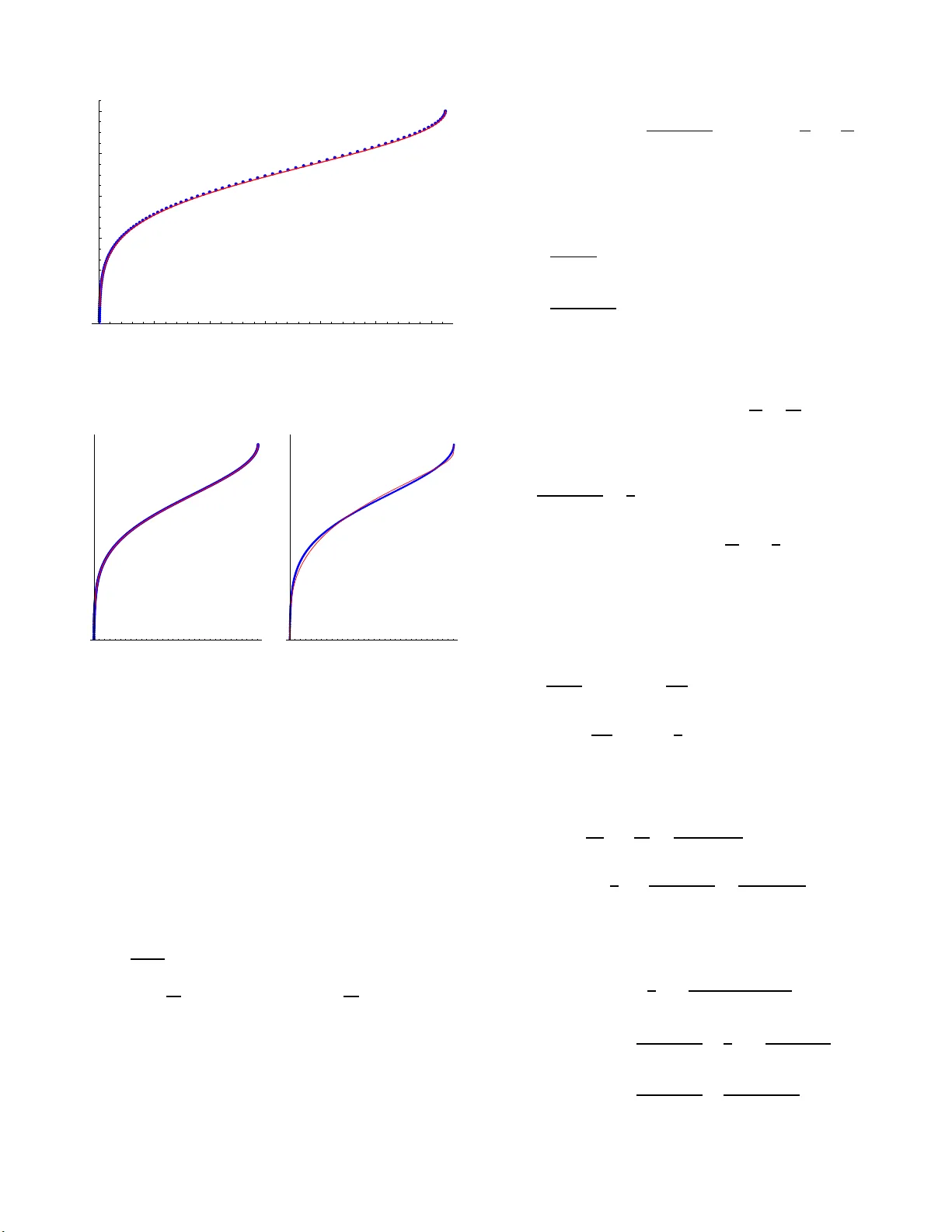
The P olyc hronak os–F rahm spin c hain of B C N t yp e and Berry–T abor’s conj ecture J.C. Barba, ∗ F. Fink el, † A. Gonz´ alez-L´ op ez, ‡ and M.A. Rodr ´ ıguez § Departamento de F ´ ısica T e´ orica I I , Universidad Complutense, 28 040 Madrid, Sp ain (Dated: March 5, 2008) W e compute the partition function of the su( m ) P olychronak os–F rahm spin chain of B C N type by means of the freezing trick. W e use th is partition function to stud y severa l statistical prop erties of the sp ectrum, whic h turn out to b e analogous to those of other spin chains of Haldane–Shastry type. In particular, w e fin d that when t he num b er of particles is sufficientl y large the level density follo ws a Gaussian distribution with great accuracy . W e also sho w that the distribution of (normalized) spacings betw een consecutive lev els is of neither Po isson nor Wigner typ e, but is qualitativ ely similar to that of the original Haldane–Sh astry spin chain. This suggests that spin chains of Haldane– Shastry type are ex ceptional integrable models, since th ey do not satisfy a w ell-known conjecture of Berry and T ab or according to which the spacings d istribu t ion of a generic integrable system should b e Poiss onian. W e derive a simple analytic expression for the cumulative spacings distribution of the B C N -type Polyc hronakos–F rahm chain using only a few essential p roperties of its sp ectrum, like the Gaussian c haracter of the level den sit y and the fact t he energy levels are equ ally spaced. This expression is in excellent agreement with t h e numerical data and, moreo ver, there is strong evidence that it can also b e applied to the Haldane–Sh astry and the Polyc hronakos–F rahm spin chains. P ACS nu mbers: 75.10.Pq, 05.30.-d, 05.45.Mt I. INTRODUCTION Solv able spin c hains often pr o vide a natural setting for testing or modeling interesting physical phenomena a nd mathematical results in such disparate fields as fractio nal statistics, r andom matrix theory or orthogo nal polynomi- als. Among these chains, those of Haldane–Shastry (HS) t yp e o ccupy a distinguis hed p osition due to their remark - able integrability and solv abilit y prop erties. The o riginal chain of this type w as indep endently introduced tw ent y years a go by Haldane [1] and Shastry [2], in an attempt to constr uct a mo del w ho se g round state co incided with Gutzwiller’s v ariational wa ve function for the Hubbar d mo del in the limit of la rge on- site interaction [3, 4, 5]. In the original HS c hain, the spins are equally-spac ed on a circle and present pa irwise in teractio ns inv ersely prop or- tional to their c hord distance. An essential feature of the spin chains of HS type is their close connection with the spin versions o f the Caloger o [6 ] and Sutherland [7, 8] mo dels, and their gen- eralizations due to Ols hanetsky and Perelomov [9]. This observ ation —alrea dy p ointed out b y Sha s try in his orig - inal pap er— was elega n tly fo r m ulated by Polychronakos in Ref. [10]. In the latter reference, the a uthor show ed that the o riginal HS chain ca n b e obtained fr o m the spin Sutherland mo del [11, 12, 13] in the strong cou- pling limit, in whic h the dynamical and spin degrees o f freedom deco uple, s o that the particles “ freeze” at the equilibrium p ositions of the scala r part of the potential. In this r e gime, the in tegr a ls of mo tion o f the spin Suther- ∗ Electronic address: jcbarba@fis.ucm.es † Electronic address: ffink el@fis.ucm.es ‡ Corresp onding author. El ectronic address: artemio@fis.ucm.es § Electronic address: rodri gue@fis.ucm.es land model directly yield fir st integrals of the HS c hain, thereby expla ining its complete integrabilit y . This pro- cedure was also applied in [10] to c o nstruct a new in te- grable spin chain related to the orig ina l Calo gero mo del. The sp ectrum of this chain w as numerically studied by F rahm [14], w ho found that the levels are gr ouped in highly degenera te multiplets. In a subsequent publica- tion, Polychronakos co mputed the partition function of this c hain (usually referred to in the literature a s the Polyc hrona kos–F r ahm chain) b y the “freezing trick” a r- gument des cribed ab ov e [15]. Interestingly , the pa rtition function o f the origina l HS chain was co mputed only very recently [16]. Both the HS and the PF (Polyc hro nak os– F rahm) chains a r e obtained from the Sutherland and Calo g ero mo dels asso ciated with the A N ro ot system in Olsha net- sky and Perelomov’s appro ach. The B C N versions of bo th c hains ha ve also been studied in the literature. More precisely , the integrability of the PF c hain of B C N t yp e was established by Y amamo to and Tsuchiya [17] using again the fr eezing trick. On the other hand, the parti- tion function of the HS chain of B C N t yp e was computed in clo sed for m in Ref. [18]. The explicit knowledge of the partition function made it p o ssible to study certain sta- tistical prop e rties o f the sp ectrum of this chain. In par- ticular, it was obser v ed that for a la rge num b er of spins the level dens it y is Gaussian. As a ma tter of fact, this prop erty also holds for the original HS c hain, as shown in Ref. [16]. The ana lysis of the distribution of the spac- ing b etw een co nsecutiv e le v els of the o r iginal HS chain was a lso undertaken in the la tter reference. Rather un- exp ectedly , it was found that this distribution is no t of Poisson type, as should b e the case for a “gener ic ” inte- grable mo del according to a long-s ta nding conjecture of Berry and T a bor [19]. This behavior has also b een re- cently rep orted for a sup ersymmetric version of the HS 2 chain [20]. The aim o f this pap er is tw ofold. In the first place, we shall co mpute in closed form the partition function of the PF chain of B C N t yp e by means o f the freezing trick. Using the par tition function, we shall per form a nu merica l study of the density of levels and the dis tri- bution of the spac ing b etw een consecutive ener gies. W e shall see that the le vel density is again Gaussian, and that the s pacings distribution is a nalogous to that of the original HS chain. In pa rticular, our res ults show that the distr ibutio n of spacings is neither Poissonian no r of Wigner type (characteristic of chaotic systems). W e shall next de r iv e a simple analytic expr ession for the cumula- tive spacings distribution, whic h r epro duces the num er- ical data with muc h gr eater accurac y than the empiric formula prop osed in Ref. [16]. In fact, we have strong nu merica l evidence that the new ex pression can a lso be applied to the HS and P F chains of A N t yp e. In view of the Berry–T abor conjecture, our results suggest tha t spin chains of HS type a re ex ceptional a mong the class of integrable mo dels. I I. THE P AR TITION FUNCTION OF THE PF CHAIN OF B C N TYPE The Hamiltonian of the (antiferromagnetic) su( m ) P F chain of B C N t yp e is defined b y H ǫ = X i 6 = j  1 + S ij ( ξ i − ξ j ) 2 + 1 + ˜ S ij ( ξ i + ξ j ) 2  + β X i 1 − ǫS i ξ 2 i , (1) where the sums run from 1 to N (as alwa ys hereafter, unless otherwise stated), β > 0, ǫ = ± 1, S ij is the op- erator whic h p ermutes the i -th and j -th spins, S i is the op erator r e v ersing the i -th spin, a nd ˜ S ij = S i S j S ij . No te that the spin op erato rs S ij and S i can b e expr essed in terms of the fundamental su( m ) spin gener a tors J α k at the site k (with the normaliz a tion tr( J α k J γ k ) = 1 2 δ αγ ) as S ij = 1 m + 2 m 2 − 1 X α =1 J α i J α j , S i = √ 2 m J 1 i . The chain sites ξ i are the co ordina tes of the unique min- im um in C = { x | 0 < x 1 < · · · < x N } of the potential U ( x ) = X i 6 = j  1 ( x − ij ) 2 + 1 ( x + ij ) 2  + X i β 2 x 2 i + r 2 4 , (2) where x ± ij = x i ± x j and r 2 = P i x 2 i . The exis tence of this minim um follows from the fact that U tends to + ∞ on the b oundary of C a nd as r → ∞ , and its uniqueness was esta blished in Ref. [21] by expressing the p otential U in terms of the log a rithm of the ground state of the B C N Caloger o mo de l H sc = − X i ∂ 2 x i + a ( a − 1) X i 6 = j  1 ( x − ij ) 2 + 1 ( x + ij ) 2  + b ( b − 1) X i 1 x 2 i + a 2 4 r 2 , (3) with b = β a and a > 1 / 2. Moreover, it can b e s hown [22] that ξ i = √ 2 y i , where y i is the i -th zero of the genera l- ized Lag uerre p olynomial L β − 1 N . F rom this fact, one can infer [23 ] that fo r N ≫ β the density of s ites (norma lized to unit y) ρ N ( x ) is given by the circula r law ρ N ( x ) = 1 2 π N p 8 N − x 2 . (4) Note tha t in this limit the sites’ densit y is independent of β and is qualitatively similar to that of the P F c hain of A N t yp e [14]. Integrating the previous equation, we obtain the implicit a symptotic rela tion 4 π k = ξ k q 8 N − ξ 2 k + 8 N a rcsin  ξ k √ 8 N  , v alid also for N ≫ β . The spin chain (1) ca n b e expressed in ter ms of the spin Calo g ero mo del of B C N t yp e H ǫ = − X i ∂ 2 x i + a X i 6 = j  a + S ij ( x − ij ) 2 + a + ˜ S ij ( x + ij ) 2  + b X i b − ǫS i x 2 i + a 2 4 r 2 (5) and its sca lar re ductio n (3) as H ǫ = H sc + a e H ǫ , (6) where e H ǫ is obtained from H ǫ replacing the chain s ites ξ by the particle s ’ co or dina tes x . Since H ǫ = − X i ∂ 2 x i + a 2 U + O ( a ) , when the coupling constant a tends to infinity the parti- cles in the spin dynamical mo del (5) conce n trate at the co ordinates of the minim um of the po ten tial U , that is at the sites ξ i of the chain (1). Thus, in the limit a → ∞ the spin and dynamical deg rees of free do m of the Hamil- tonian (5) decouple, s o that by Eq. (6) its eige nv alues are approximately given by E ǫ ij ≃ E sc i + a E ǫ j , a ≫ 1 , (7) where E sc i and E ǫ j are tw o arbitra ry eigenv alues of H sc i and H ǫ , resp ectively . The asymptotic r elation (7) imme- diately yields the following ex act form ula for the par tition function Z ǫ of the chain (1): Z ǫ ( T ) = lim a →∞ Z ǫ ( aT ) Z sc ( aT ) , (8) 3 where Z ǫ and Z sc are the pa r tition functions of H ǫ and H sc , resp ectively . W e shall next ev aluate the par titio n function Z ǫ of the chain (1) by computing the par tition functions Z ǫ and Z sc in Eq. (8). In o rder to deter mine the s pectra of the corr espo nding Hamiltonians H ǫ and H sc , following Ref. [16] we intro duce the auxiliary op erato r H ′ = − X i ∂ 2 x i + X i 6 = j  a ( x − ij ) 2 ( a − K ij ) + a ( x + ij ) 2 ( a − e K ij )  + X i b x 2 i ( b − K i ) + a 2 4 r 2 , (9) where K ij and K i are co ordinate p ermutation and sign reversing op erators , defined by ( K ij f )( x 1 , . . . , x i , . . . , x j , . . . , x N ) = f ( x 1 , . . . , x j , . . . , x i , . . . , x N ) , ( K i f )( x 1 , . . . , x i , . . . , x N ) = f ( x 1 , . . . , − x i , . . . , x N ) , and e K ij = K i K j K ij . W e then hav e the obvious rela tions H ǫ = H ′   K ij →− S ij ,K i → ǫS i , (10a) H sc = H ′   K ij ,K i → 1 . (10b) On the other hand, the spectrum of H ′ can be easily computed by noting that this op erato r ca n b e written in terms of the rational Dunkl op erator s of B C N t yp e [24] J − i = ∂ x i + a X j 6 = i  1 x − ij (1 − K ij ) + 1 x + ij (1 − e K ij )  + b x i (1 − K i ) , i = 1 , . . . , N , (11) as follows [2 5]: H ′ = µ h − X i  J − i  2 + a X i x i ∂ x i + E 0 i µ − 1 , (12) where µ ( x ) = e − a 4 r 2 Y i | x i | b · Y i · · · > n N . (ii) s i > s j whenever n i = n j and i < j . (iii) s i > 0 for all i , and s i > 0 if ( − 1) n i = − ǫ . The fir st tw o conditions are a c o nsequence of the anti- symmetry of the states (18) under pa rticle p ermutations, while the last condition is due to the fact that these states must ha ve par it y ǫ under s ign reversals. Since K ij Λ ǫ = − S ij Λ ǫ and K i Λ ǫ = ǫS i Λ ǫ , it follows that H ǫ Λ ǫ = H ′ Λ ǫ . Using this identit y and the fact that H ′ obviously commutes with Λ ǫ , from E q. (16) we easily obtain H ǫ ψ n , s = H ′ ψ n , s = Λ ǫ  ( H ′ φ n ) | s i  = E ′ n ψ n , s + X | m | < | n | c mn ψ m , s . Thu s H ǫ is represe nted by a n upper triangular matr ix in the ba sis (18), or de r ed accor ding to the degree | n | . The diagonal elements of this matrix are given by E ǫ n , s = a | n | + E 0 , (19) where n a nd s satisfy conditions (i)–(iii) above. Note that, although the numerical v alue of E ǫ n , s is indep endent of s , the degeneracy of each level clearly depends on the spin throug h the latter conditions. T urning next to the sc a lar Hamiltonian H sc , in view of Eq. (1 0b) we now need to consider s calar functions of the form ψ n ( x ) = Λ s φ n ( x ) , (20) where Λ s is the sy mmetrizer with resp ect to b oth p er- m utations and sign reversals. Thes e functions form a 4 (non-orthono r mal) bas is of the Hilb ert space of H sc pro- vided that n i = 2 k i are even in teger s and k 1 > · · · > k N . Just as b efore, the matrix of the scala r Hamiltonian H sc in the basis (20) ordered by the degre e is upp er triang u- lar, with diagonal elements E sc n also given by the RHS of (19). Let us nex t compute the pa rtition functions Z sc and Z ǫ of the mo dels (3 ) and (5). T o beg in with, fro m no w on we shall drop the co mmon gr ound state energy E 0 in bo th mo dels, since by Eq . (8) it do es not contribute to the partition function Z ǫ . With this conv ention, the partition function o f the sca lar Ha miltonian H sc is given by Z sc ( aT ) = X k 1 > ··· > k N > 0 q 2 | k | , where q = e − 1 / ( k B T ) . The previous sum can b e ev aluated by expr essing it in terms o f the differences p i = k i − k i +1 , i = 1 , . . . , N − 1, with p N ≡ k N . Since k j = N P i = j p i , we easily obtain Z sc ( aT ) = X p 1 ,...,p N > 0 q 2 N P j =1 N P i = j p i = X p 1 ,...,p N > 0 q 2 N P i =1 ip i = Y i X p i > 0 ( q 2 i ) p i = Y i (1 − q 2 i ) − 1 . (21) In order to compute the partition function of the spin Hamiltonian H ǫ , we shall first a ssume that m is even, so that condition (iii) simplifies to (iii ′ ) s i > 0 for all i . As neither the v alue o f E ǫ n , s nor co nditions (i), (ii) and (iii ′ ) dep end o n ǫ , in this ca se the partition functions Z ǫ and Z ǫ cannot depend o n ǫ . Hence fro m now on w e shall drop the sup e rscript ǫ when m is even, wr iting simply Z and Z . By E q. (19), after dr opping E 0 the par tition function of the Hamiltonian (5) can b e wr itten as Z ( aT ) = X n 1 > ··· > n N > 0 d n q | n | , (22) where the s pin degenera cy factor d n is the num b er of s pin states | s i s atisfying conditions (ii) and (iii ′ ). W riting n =  ν 1 z }| { k 1 , . . . , k 1 , . . . , ν r z }| { k r , . . . , k r  , k 1 > · · · > k r > 0 , by conditions (ii) and (iii ′ ) we hav e d n = r Y i =1  m/ 2 ν i  ≡ d ( ν ) , ν = ( ν 1 , . . . , ν r ) . (23) Note that P r i =1 ν i = N , so that the multiindex ν ca n be regar ded as an element o f the set P N of partitions of N (taking order into account). With the pr e vious no tation, Eq. (22) b ecomes Z ( aT ) = X ν ∈P N d ( ν ) X k 1 > ··· >k r > 0 q r P i =1 ν i k i = X ν ∈P N d ( ν ) X p 1 ,...,p r − 1 > 0 p r > 0 q r P i =1 ν i r P j = i p j = X ν ∈P N d ( ν ) X p 1 ,...,p r − 1 > 0 p r > 0 r Y j =1 q p j j P i =1 ν i = q − N X ν ∈P N d ( ν ) r Y j =1 q N j 1 − q N j , (24) where N j = j X i =1 ν i . F rom E qs. (8), (21 ) and (24) we finally obtain the follow- ing explicit expressio n for the partition function of the su( m ) PF chain o f B C N t yp e in the c ase of ev en m : Z ( T ) = q − N Y i (1 − q 2 i ) X ν ∈P N d ( ν ) ℓ ( ν ) Y j =1 q N j 1 − q N j , (2 5) where ℓ ( ν ) = r is the num b e r of comp onents of the mul- tiindex ν . F or instance, for spin 1 / 2 w e hav e ν i = 1 for all i , a nd therefor e r = N , d ( ν ) = 1 a nd N j = j , so that the previo us formula simplifies to Z ( T ) = q 1 2 N ( N − 1) Y i (1 + q i ) , m = 2 . (26) Thu s, for spin 1 / 2 the s pectrum of the chain (1) is g iv en by E j = 1 2 N ( N − 1 ) + j , j = 0 , 1 , . . . , 1 2 N ( N +1 ) , (27) and the degener acy of the energy E j is the n umber Q N ( j ) of par titions of the integer j into distinct pa rts no lar ger than N (with Q N (0) ≡ 1 ). F or j 6 N this nu mber coincides with the num ber Q ( j ) of partitions o f j into distinct parts, which has b een extensively s tudied in the mathematical literatur e [26]. It is a ls o interesting to ob- serve that the partition function (26) is closely related to Ramanujan’s fifth or der mo ck theta function [27] ψ 1 ( q ) = ∞ X N =0 q N Z N ( q ) , where Z N ( q ) denotes the RHS of Eq . (26 ). Equation (26) shows that for spin 1 / 2 the c hain (1) is equiv alen t to a sy stem of N species o f nonin teracting 5 fermions (with v acuum energy E 0 = N ( N − 1) / 2), whose effective Hamiltonian is giv en by H eff = E 0 + N X i =1 E i b † i b i . Here b i (resp. b † i ) is the a nnihila tion (resp. creation) op- erator of the i -th sp ecies of fermion, a nd E i = i its energy . A similar result was o btained in Ref. [28] for the sup ersymmetric su(1 | 1) (ferromag ne tic) HS chain, al- though in the latter case the ener gy of the i -th fermion is E i = i ( N − i ) (the disp ersion relation of the orig ina l Haldane–Shastr y chain). Let us consider no w the cas e o f o dd m . In this case, it is conv enient to slightly mo dify c o ndition (i) ab ov e by first grouping the compo nen ts of n with the same parity and then order ing separ ately the even and o dd comp onents. In other words, we shall write n = ( n e , n o ), where n e =  ν 1 z }| { 2 k 1 , . . . , 2 k 1 , . . . , ν s z }| { 2 k s , . . . , 2 k s  , n o =  ν s +1 z }| { 2 k s +1 + 1 , . . . , 2 k s +1 + 1 , . . . , ν r z }| { 2 k r + 1 , . . . , 2 k r + 1  , and k 1 > · · · > k s > 0 , k s +1 > · · · > k r > 0 . By co nditions (ii) and (iii), the spin degener acy factor is now d ǫ n = s Y i =1  m + ǫ 2 ν i  · r Y i = s +1  m − ǫ 2 ν i  ≡ d ǫ s ( ν ) . (28) Calling ˜ N j = j X i = s +1 ν i , j = s + 1 , . . . , r , and pro ceeding as b efore, we obtain Z ǫ ( aT ) = X ν ∈P N r X s =0 d ǫ s ( ν ) X k 1 > ··· >k s > 0 k s +1 > ··· >k r > 0 q s P i =1 2 ν i k i q r P i = s +1 ν i (2 k i +1) = X ν ∈P N r X s =0 d ǫ s ( ν ) q ˜ N r " X k 1 > ··· >k s > 0 q s P i =1 2 ν i k i # × " X k s +1 > ··· >k r > 0 q r P i = s +1 2 ν i k i # = X ν ∈P N ℓ ( ν ) X s =0 d ǫ s ( ν ) q − ( N + N s ) s Y j =1 q 2 N j 1 − q 2 N j × ℓ ( ν ) Y j = s +1 q 2 ˜ N j 1 − q 2 ˜ N j . (29) Substituting the previous expre ssion a nd (21) into (8), we immediately deduce the following ex plicit for m ula for the partition functions of the su( m ) PF chain of B C N t yp e for odd m : Z ǫ ( T ) = Y i (1 − q 2 i ) X ν ∈P N ℓ ( ν ) X s =0 d ǫ s ( ν ) q − ( N + N s ) × s Y j =1 q 2 N j 1 − q 2 N j · ℓ ( ν ) Y j = s +1 q 2 ˜ N j 1 − q 2 ˜ N j . (30) Although w e hav e chosen, for definiteness, to study the a n tiferromag netic chain (1), a similar analysis can be per formed for its fer romagnetic counterpart H ǫ F = X i 6 = j  1 − S ij ( ξ i − ξ j ) 2 + 1 − ˜ S ij ( ξ i + ξ j ) 2  + β X i 1 − ǫS i ξ 2 i . (31) Since now H ǫ F = H ′   K ij → S ij ,K i → ǫS i , (32) we must replace the op erator Λ ǫ in E q. (1 8 ) by the pro - jector on states symmetric under simultaneous p ermut a- tions of the pa rticles’ s patial a nd s pin co or dinates, a nd with par it y ǫ under sign reversal of co or dinates and spin. Hence condition (ii) ab ov e o n the basis states ψ n , s should now read (ii ′ ) s i > s j whenever n i = n j and i < j . As a result, the degenera cy factors d ( ν ) and d ǫ ( ν ) in Eqs. (23) and (28) should b e replaced by their “ boso nic” versions d F ( ν ) = r Y i =1  m 2 + ν i − 1 ν i  , d ǫ F ( ν ) = s Y i =1  m + ǫ 2 + ν i − 1 ν i  · r Y i = s +1  m − ǫ 2 + ν i − 1 ν i  . Therefore the partition function of the fer romagnetic su( m ) PF chain of B C N t yp e (31) is still given by Eq . (25) (for even m ) or (30) (for o dd m ), but with d ( ν ) and d ǫ ( ν ) replaced resp ectively by d F ( ν ) and d ǫ F ( ν ). On the other hand, the chains (1) a nd (31) are ob vi- ously related by H ǫ F + H − ǫ = 2  X i 6 = j  ( ξ i − ξ j ) − 2 + ( ξ i + ξ j ) − 2  + β X i ξ − 2 i  . The RHS of this equation clearly c oincides with the largest eig e n v alue E max of the antiferromagnetic chains H ǫ , whose corres ponding eigenv ectors ar e the spin sta tes symmetric under p ermutations and with par it y ǫ under spin reversal. This eigenv alue is most easily c o mputed for the spin 1 / 2 chains, since in this c a se the sp ectrum is explicitly given in Eq. (2 7). W e th us obtain E max = 1 2 N ( N − 1) + 1 2 N ( N + 1) = N 2 , (33) 6 so that H ǫ F = N 2 − H − ǫ . Hence the partition functions Z ǫ and Z ǫ F of H ǫ and H ǫ F satisfy the r e ma rk able identit y Z ǫ F ( q ) = q N 2 Z − ǫ ( q − 1 ) . This is a manifestation o f the bo son-fermion duality dis- cussed in detail in Ref. [29] for the su( m | n ) s up ersy m- metric HS s pin chain, since the ferromag netic (r esp. a n- tiferromagnetic) chain can be reg arded as purely bo sonic (resp. fermionic). F o r instance, using the latter identit y and Eq. (26) we eas ily obtain the following expressio n for the partition function o f the ferromag netic spin 1 / 2 chains: Z F ( T ) = Y i (1 + q i ) , m = 2 . (34) (Note that, a s in the an tiferro magnetic case, Z ǫ F is actu- ally indep enden t of ǫ for even m .) This is, a gain, the par- tition function of a system of N s pecies o f free fermions of energ y E i = i , but no w the v acuum ener gy v anishes. Equation (25) for the pa rtition function of the antif er- romagnetic c hains with even m ca n b e easily simplified to Z ( T ) = Y i (1 + q i ) X ν ∈P N d ( ν ) q ℓ ( ν ) − 1 P j =1 N j N − ℓ ( ν ) Y j =1 (1 − q N ′ j ) , where the p ositive integers N ′ j are defined by  N ′ 1 , . . . , N ′ N − ℓ ( ν )  =  1 , . . . , N − 1  −  N 1 , . . . , N ℓ ( ν ) − 1  . The s um in the RHS is easily recog nized as the parti- tion function Z ( A ) ( T ; m/ 2) of the s u( m/ 2) (a n tiferro- magnetic) PF chain of A N t yp e [20]. W e thus obtain the remar k a ble factoriza tion Z ( T ; m ) = Z F ( T ; 2) · Z ( A ) ( T ; m/ 2) , m ∈ 2 N , (35) where the second argument in Z and Z F denotes the nu mber of internal degrees o f freedom. Replacing d ( ν ) by d F ( ν ) in Eq. (25) w e obtain a similar factoriza tion for the partition function of the ferr omagnetic chains: Z F ( T ; m ) = Z F ( T ; 2) · Z ( A ) F ( T ; m/ 2) , m ∈ 2 N . (3 6) Thu s, for even m the PF chains of B C N t yp e (1) a nd (31) can b e desc ribed b y an effective mo del of t wo simpler noninteracting c hains. This remark able prop erty , whic h to the be s t of our knowledge is unique among the class of chains of Halda ne–Shastry type, cer tainly deserves fur- ther inv estigation. I II. SP A CINGS DISTRI BUTION AND THE BERR Y –T ABOR CONJECTURE F or fix ed v alues of the num b e r o f particles N and the int erna l deg r ees o f freedom m , it is stra igh tforward to obtain the sp ectrum of the chain (1 ) b y expanding in powers of q the expressions (25) or (30) for its partition function. In this w ay , we hav e b e en able to compute the sp ectrum of the latter chain for r elatively lar ge v alues of N (for instance, up to N = 22 for m = 3). Our calcu- lations co nclusively show that the sp ectrum consists of a set of consecutive in tegers. F or ev en m , this o bserv a- tion follows immediately from the expr ession (34)-(35) and the fact the the energies of the PF chain of A N t yp e are also consecutive in tegers. F or o dd m we hav e b een unable to deduce this pro perty from Eq . (30) for the par- tition function, although we hav e verified it numerically for many different v alues o f N and m . Our computations also ev idence that for N & 10 the level densit y (norma lized to unity) ca n b e approximated with grea t accurac y by a normal distribution g ( E ) = 1 √ 2 π σ e − ( E − µ ) 2 2 σ 2 , (37) where µ and σ are resp ectively the mean and the v aria nc e of the energ y . F or instance, in Fig. 1 we compar e the cum ulative le vel density F ( E ) = m − N X i ; E i 6 E d i , where E i is the i -th energy and d i its degener acy , with the cumulativ e Gaussian density G ( E ) = Z E −∞ g ( E ′ ) d E ′ = 1 2  1 + erf  E − µ √ 2 σ  (38) for N = 15 and m = 2. Note, in this resp ect, that 140 160 180 200 220 1.0 0.2 0.4 0.6 0.8 Ɛ ( Ɛ ) F , ( Ɛ ) G FIG. 1: Cumulativ e distribution functions F ( E ) (at its dis- conti nuity p oints) and G ( E ) (contin uous red line) for N = 15 and spin 1 / 2. 7 the approximately Gaussian character of the level densit y has already b een verified for other chains of HS type , like the original Haldane–Shastr y chain [1 6], its su( m | n ) sup e rsymmetric version [2 0], and the HS s pin chain of B C N t yp e [18]. The mean ener g y µ a nd its standard deviatio n σ 2 , which b y the previous disc ussion c hara cterize the appro x- imate le vel densit y of the chain (1) for large N , ca n b e computed in closed form. Indeed, in App endix A we show that µ = 1 2  1 + 1 m  N 2 − N 2 m (1 + ǫ p ) , (39) σ 2 = N 36 (4 N 2 + 6 N − 1)  1 − 1 m 2  + N (1 − p ) 4 m 2 , (4 0) where p ∈ { 0 , 1 } is the par it y of m . Th us, when N tends to infinit y µ and σ 2 resp ectively diverge as N 2 and N 3 , as for the orig inal Polyc hronakos–F ra hm chain [35]. By contrast, it is known that µ ∼ N 3 and σ 2 ∼ N 5 for the trigonometric HS c hains of both A N [16] and B C N [18] t yp es. It is also interesting to observe that the standard deviation of the energy is indep endent o f ǫ even for o dd m , when the sp ectrum do es dep end o n ǫ according to the previous section’s re sults on the pa r tition function. W e have next studied the pr obabilit y density p ( s ) of the spacing s b et ween c o nsecutive (unfolded) levels of the chain (1). F or many imp ortant integrable systems it is known that p ( s ) is Poissonian [30, 31], in agre e ment with a well-known conjecture of Ber r y a nd T abor [19]. On the other hand, it has b een recently shown tha t for the HS chain of A N t yp e [16] (and its sup ersymmetr ic extension [2 0]) the cumulativ e density P ( s ) = R s 0 p ( x )d x is well appr oximated b y an empiric law of the form e P ( s ) =  s s max  α " 1 − γ  1 − s s max  β # , (41 ) where s max is the larg est normaliz ed spacing and α, β ar e adjustable parameter s in the in terv al (0 , 1). The param- eter γ is fixed b y requiring that the av era ge spacing b e equal to 1 , with the result γ =  1 s max − α α + 1 . B ( α + 1 , β + 1) , (42) where B is Euler’s Beta function. Thus, the cumulative density of spacings for the HS c hains of A N t yp e follows neither Poisson’s no r Wig ne r ’s law P ( s ) = 1 − e − π s 2 / 4 , characteristic of a c haotic system. O ur aim is to ascerta in whether the cumulativ e density of spacings for the PF chain of B C N t yp e (1) resembles that o f the A N -type HS chain, or is ra ther Poissonian a s expec ted for a g e ne r ic int egr able mo del. In o rder to compare the spacing s distributions of spec - tra with differen t le vel densities, it is necessa ry to tra ns- form the “raw” sp ectrum b y applying what is known as the unfolding ma pping [32]. This mapping is defined b y decomp osing the cumulativ e lev el densit y F ( E ) a s the sum of a fluctuating part F f l ( E ) and a co ntin uous par t η ( E ), which is then used to transfor m each energy E i , i = 1 , . . . , n , into an unfolded energy η i = η ( E i ). In this wa y one o btains a unifor mly distributed sp ectrum { η i } n i =1 , r egardless of the initial level density . One finally considers the nor malized s pacings s i = ( η i +1 − η i ) / ∆, where ∆ = ( η n − η 1 ) / ( n − 1) is the mean spacing of the unfolded energ ies, so that { s i } n − 1 i =1 has unit mean. By the a bov e discussion, in our cas e we ca n take the un- folding mapping η ( E ) as the cumulative Gaussian distri- bution (38), with parameters µ and σ r e spectively given by (39) and (40). Just as for the level densit y , in o r der to compar e the discr ete distribution function p ( s ) with a con tinuous distribution it is more conv enient to work with the cumulativ e spa cings distribution P ( s ). Our computations show that for a wide r ange of v alues of N , m and ǫ = ± 1 , the distribution P ( s ) is well approximated by the empiric law (41) with suitable v alues of α and β . F or instance, for N = 2 0 and m = 2 the lar gest spacing is s max = 3 . 1 3, and the least-squa res fit parameters α a nd β are resp ectively 0 . 29 and 0 . 2 4, with a mean sq ua re err or of 6 . 0 × 10 − 4 (see Fig. 2). Thus the PF spin chain of B C N 0.0 0.5 1.0 1.5 2.0 2.5 3.0 s 0.2 0.4 0.6 0.8 1.0 P ( s ) FIG. 2: Cumulativ e sp acings distribution P ( s ) and its ap- proximati on e P ( s ) (con tinuous red line) f or N = 20 and m = 2. F or conv enience, we hav e also represen ted Poiss on’s (green, long dashes) and Wigner’s (green, short dashes) cumulativ e distributions. t yp e b ehav es in this resp ect as the HS chain of A N t yp e, and unlike most known in tegr able sys tems. In fact, we hav e also studied the spa cings’ dis tr ibution of the o rig- inal ( A N -type) PF chain, obtaining c ompletely similar results [3 5]. These r esults (and also those of Re f. [20]) suggest that a s pacings distr ibutio n qualita tively simila r to the empiric law (41) is ch ar acteristic of all spin chains of HS type. Our next ob jective is to explain this characteristic be - havior o f the cumulativ e spacings distribution P ( s ) of the chain (1) using only a few essential prop erties of its sp ec- trum. W e shall find a simple analytic expression without 8 any adjustable parameters approximating P ( s ) even bet- ter than the empiric law (41). Moreover, we have s trong nu merica l evidence that the new expressio n also pr o vides a v ery accurate appro ximation to the cumulativ e spacings distribution of the original HS and PF chains. Consider, to b egin with, any sp ectrum E 1 ≡ E min < · · · < E n ≡ E max ob eying the following conditions: (i) The energies ar e equispaced, i.e., E i +1 − E i = δ for i = 1 , . . . , n − 1. (ii) The level density (normalized to unity) is approxi- mately Gaus s ian, cf. E q . (37 ). (iii) E n − µ , µ − E 1 ≫ σ . (iv) E 1 and E n are approximately sy mmetric with respect to µ , namely |E 1 + E n − 2 µ | ≪ E n − E 1 . As discussed above, the s pectrum of the chain (1) satisfies the first condition with δ = 1, while condition (ii) holds for sufficiently la rge N . As to the third conditio n, from Eqs. (3 3), (39), (40), (B1) and (B2) it follows that bo th ( E n − µ ) /σ and ( µ − E 1 ) /σ grow as N 1 / 2 when N → ∞ . The last condition is also satisfied for large N , s ince by the equa tions just q uoted |E 1 + E n − 2 µ | = O ( N ) while E n − E 1 = O ( N 2 ). F rom conditions (i) and (ii) it follows that η i +1 − η i = G ( E i +1 ) − G ( E i ) ≃ G ′ ( E i ) δ = g ( E i ) δ . On the other ha nd, by condition (iii) we have η n = G ( E n ) ≃ 1 , η 1 = G ( E 1 ) ≃ 0 , so that ∆ = 1 / ( n − 1 ). Thus s i = η i +1 − η i ∆ ≃ W g ( E i ) = W √ 2 π σ e − ( E i − µ ) 2 2 σ 2 , (43) where W ≡ ( n − 1) δ = E n − E 1 (44) on account o f the first condition. The cumulativ e prob- ability density P ( s ) is by definition the quotient of the nu mber of normalized s pacings s i 6 s by the total num- ber of spacings, tha t is, P ( s ) = #( s i 6 s ) n − 1 . By Eq. (43), #( s i 6 s ) = #  E 1 6 E i 6 E −  + #  E + 6 E i < E n  , (45) where E ± = µ ± √ 2 σ r log  s max s  (46) are the ro ots of the equation s = W g ( E ) expr e ssed in terms of the maxim um normaliz ed spa c ing s max = W √ 2 π σ . (47) Using the first condition to es timate the RHS of Eq. (45) we easily obta in P ( s ) ≃ 1 W  max( E − − E 1 , 0) + max ( E n − E + , 0)  . ( 48) In fact, we can r eplace the latter approximation to P ( s ) by the simpler o ne P ( s ) ≃ 1 W  E − − E 1 + E n − E +  , (49) since the err or inv olved is b ounded by 1 W   E 1 + E n − 2 µ   , which is v anishingly small b y co ndition (iv). Substitut- ing the explicit expression (46) for E ± int o Eq. (49) and using (44) and (47) we finally obtain P ( s ) ≃ 1 − 2 √ π s max r log  s max s  . (5 0 ) The RHS o f this remark able expre ssion dep ends only on the qua n tity s max , whic h for the PF chain o f B C N t yp e is completely deter mined as a function o f N and m by Eqs. (3 3), (44), (47 ) and (B1 )-(B2). In particular , fo r large N we hav e the asymptotic ex pr ession s max = 3 √ 2 π r m − 1 m + 1 N 1 / 2 + O  N − 1 / 2  . Our numerical c o mputations indicate that Eq. (5 0) is in excellent ag reement with the da ta for a bro ad range of v alues of N , m and ǫ = ± 1, providing muc h gr eater accu- racy than the e mpir ic form ula (41). F or instance, for N = 20 a nd m = 2 we hav e s max = 6 p 35 / (41 π ) ≃ 3 . 1276 5, which differs fr om the numerically computed maximum spacing by 4 . 5 × 10 − 4 . In Fig. 3 we co mpare the cor- resp onding cumulative spacings dis tribution with its ap- proximation (50) using the ab ov e v alue of s max . The mean square err or is in this cas e 2 . 2 × 10 − 5 , smaller than that of the empiric law (41) by more tha n a n or der of magnitude. A natural question in view of these results is to what extent the approximation (50) is applicable to other spin chains o f HS t yp e. F or the P F chain of A N t yp e, one can chec k that the sp ectrum satis fie s co nditions (i)–(iv) o f this s ection, and in fact w e have verified that (50 ) holds with r e mark able acc uracy in this case [35]. The situation is less clear for the o riginal HS chain, who se sp ectrum is certainly not e q uispaced [16]. Nevertheless, our c o mpu- tations show that the formula (50) still fits the numerical data muc h b etter than our previous approximation (41), a fact clear ly deserving further study . As an illustra tio n, in Fig. 4 we compa r e the cumulativ e spacings distribu- tion of the or iginal HS chain with its approximations (41) and (50) for N = 25 a nd m = 2. It is apparent that the new expressio n (50) provides a mor e accurate approxima- tion to the numerical data than the empiric formula (41) (their resp ective mean square erro rs a re 1 . 8 × 10 − 5 and 5 . 8 × 10 − 4 ). 9 0.0 0.5 1.0 1.5 2.0 2.5 3.0 s 0.2 0.4 0.6 0.8 1.0 P ( s ) FIG. 3: Cumulativ e spacings distribution P ( s ) and its ana- lytic approximation (50) (contin uous red line) for N = 20 and m = 2. 0.0 0.5 1.0 1.5 2.0 2.5 3.0 s 0.2 0.4 0.6 0.8 1.0 P ( s ) 0.0 0.5 1.0 1.5 2.0 2.5 3.0 s 0.2 0.4 0.6 0.8 1.0 P ( s ) FIG. 4: Cumulativ e spacings distribut ion P ( s ) for the HS chai n of A N type in th e case of N = 25 and m = 2, com- pared to its contin uous ap p ro ximations (50) (left) and (41) (right). In b oth cases, th e th in (red ) line corresp onds to the conti nuous approximatio n. APPENDIX A: COMPUT A TION OF µ AND σ 2 In this app endix we shall compute in clo sed form the mean ene r gy µ of the spin chain (1) and its standard deviation σ 2 as functions of the num ber of particles N and internal degr ees o f freedo m m . In the first plac e , using the formulas for the traces of the o pera tors S ij , ˜ S ij and S i in Ref. [18] w e e asily obtain µ = tr H ǫ m N =  1 + 1 m  X i 6 = j ( h ij + ˜ h ij ) +  1 − ǫ p m  X i h i , ( A1) where p is the pa rit y of m and h ij = ( ξ i − ξ j ) − 2 , ˜ h ij = ( ξ i + ξ j ) − 2 , h i = β ξ − 2 i . The sums a pp earing in Eq . (A1) can b e e xpressed in terms of sums in volving the zeros y i = ξ 2 i / 2, 1 6 i 6 N , of the Lague r re p olynomial L β − 1 N as follows: X i 6 = j ( h ij + ˜ h ij ) = X i 6 = j 2 y i ( y i − y j ) 2 , X i h i = β 2 X i 1 y i . (A2) The la tter sums can b e easily computed using the fol- lowing iden tities satisfied by the zeros y i , which can be found in Ref. [33]: X j,j 6 = i 2 y i y i − y j = y i − β , (A3) X j,j 6 = i 12 y 2 i ( y i − y j ) 2 = − y 2 i + 2(2 N + β ) y i − β ( β + 4) . (A4) Indeed, from the firs t of these identities we easily obtain X i y i = N ( N + β − 1) , X i 1 y i = N β , (A5) so that, by E q. (A4), X i 6 = j 2 y i ( y i − y j ) 2 = 1 6  − X i y i + 2 N (2 N + β ) − β ( β + 4) X i 1 y i  = 1 2 N ( N − 1) . Combining the las t tw o equations with (A1) and (A2) we immediately ar rive at Eq. (39) for the le vel density µ . T urning now to the standard deviation of the energy σ 2 , from Eq s. (66 )–(68) in Ref. [1 8] we hav e σ 2 = tr H 2 ǫ m N − µ 2 =  1 − 1 m 2  2 X i 6 = j  h 2 ij + ˜ h 2 ij  + X i h 2 i  + 4 m 2 (1 − p )  1 4 X i h 2 i − X i 6 = j h ij ˜ h ij  . (A6) All of the sums appea ring in the latter expression can b e readily ev aluated. Indeed, w e hav e X i h 2 i = β 2 4 X i 1 y 2 i = N ( N + β ) 4( β + 1) (A7) X i 6 = j h ij ˜ h ij = 1 4 X i 6 = j 1 ( y i − y j ) 2 = N ( N − 1) 16( β + 1) , (A8) where we hav e used Eqs. (15 ) a nd (17) from Ref. [33]. On the other ha nd, X i 6 = j  h 2 ij + ˜ h 2 ij  = 1 2 X i 6 = j y 2 i + y 2 j + 6 y i y j ( y i − y j ) 4 = 2 X i 6 = j y 2 i + y 2 j ( y i − y j ) 4 − 3 2 X i 6 = j 1 ( y i − y j ) 2 = 4 X i 6 = j y 2 i ( y i − y j ) 4 − 3 N ( N − 1) 8( β + 1) , (A9) 10 while from [3 4, Thm. 5.1] it follows that 720 X i 6 = j y 2 i ( y i − y j ) 4 = X i y 2 i − 4(2 N + β ) X i y i + 2 N  8 N 2 + 2(4 N − 1) β + 3 β 2  − 4(2 N + β )( β 2 − 2 β − 18) X i 1 y i + β ( β 3 − 4 β 2 − 104 β − 144) X i 1 y 2 i . (A10) All the sums in the right-hand s ide of the latter expres- sion have alr eady b een ev aluated in Eqs. (A5) a nd (A7), except the first one. In order to compute this sum, we m ultiply E q. (A3) b y y i and sum o ver i , obtaining X i 6 = j 2 y 2 i y i − y j = X i 6 = j y 2 i − y 2 j y i − y j = X i 6 = j ( y i + y j ) = 2( N − 1) X i y i = X i y 2 i − β X i y i , and hence, by E q. (A5 ), X i y 2 i = N ( N + β − 1)(2 N + β − 2) . (A11 ) Substituting the v a lue o f the latter sum in Eq. (A10) a nd using (A5) and (A7) we obta in X i 6 = j y 2 i ( y i − y j ) 4 = N ( N − 1)  (2 N + 5) β + 2 N + 14  144( β + 1) . (A12) Equation (4 0) now follows by inserting (A7), (A8) and (A9)-(A12) into E q. (A6) . APPENDIX B: COMPUT A TION OF THE MINIMUM ENERGY In this app endix we shall obtain an e x plicit e x pression for the minim um e ner gy E ǫ min of the spin chain (1). O ur starting point is E q. (7), which implies that E ǫ min is given by E ǫ min = lim a →∞ 1 a  E ǫ min − E sc min  in ter ms of the minim um energies E sc min and E ǫ min of the scalar and spin dynamical mo dels (3) and (5 ), r espec - tively . By the disc us sion in Section I I (cf. E q. (19)), E ǫ min is the minim um v a lue of | n | , where n is any m ultiindex compatible with conditions (i)–(iii) in the latter section. F rom these conditions it follows that the multiindex n minimizing | n | is given by n =  l z }| { k , . . . , k , l k − 1 z }| { k − 1 , . . . , k − 1 , . . . , l 0 z }| { 0 , . . . , 0  , where 0 6 l < l k and l i is given by l i =        m 2 , m even m + ǫ 2 , m o dd and i ev en m − ǫ 2 , m and i o dd . In v iew o f the ab ov e expressio n, it is co n venien t to treat separately the cases of even a nd o dd m . F or even m , w e hav e l i = m 2 for all i , so that k = ⌊ 2 N /m ⌋ , l = N mo d m 2 , and E ǫ min = m 2 k − 1 X i =1 i + l k = m 4 k ( k − 1) + l k = N 2 m − N 2 + l ( m − 2 l ) 2 m ( m even) . (B1) Suppo se now that m is o dd. If k = 2 j is a n even n umber, then l 0 = l 2 = · · · = l 2 j − 2 = m + ǫ 2 , l 1 = l 3 = · · · = l 2 j − 1 = m − ǫ 2 and thus N = j m + l , so that j = ⌊ N/ m ⌋ , l = ( N mo d m ) < l 2 j = m + ǫ 2 . The minim um energy in this ca se is th us given by E ǫ min = m + ǫ 2 j − 1 X i =0 2 i + m − ǫ 2 j − 1 X i =0 (2 i + 1 ) + 2 j l = mj ( j − 1) + j m − ǫ 2 + 2 j l = N 2 m − N ( m + ǫ ) 2 m + l ( m + ǫ − 2 l ) 2 m . On the other hand, if k = 2 j + 1 is odd then l 0 = l 2 = · · · = l 2 j = m + ǫ 2 , l 1 = l 3 = · · · = l 2 j − 1 = m − ǫ 2 and thus N = j m + l + m + ǫ 2 , with 0 6 l < l 2 j +1 = m − ǫ 2 . Calling l ′ = l + m + ǫ 2 we hav e j = ⌊ N/ m ⌋ , l ′ = ( N mod m ) > m + ǫ 2 , and E ǫ min = m + ǫ 2 j X i =0 2 i + m − ǫ 2 j − 1 X i =0 (2 i + 1 ) + (2 j + 1)  l ′ − m + ǫ 2  = mj ( j − 1) + j m − ǫ 2 + 2 j l ′ + l ′ − m + ǫ 2 = N 2 m − N ( m + ǫ ) 2 m + ( l − m )( m + ǫ − 2 l ) 2 m . Hence we c an express the minimum ener gy for o dd m in a unified wa y as E ǫ min = N 2 m − N ( m + ǫ ) 2 m + 1 2 m  l − m θ (2 l − m − ǫ )  × ( m + ǫ − 2 l ) ( m o dd) , (B2) 11 where l = N mo d m and θ ( x ) = 1 for x > 0 and 0 o therwise. ACKNO WLEDGMENTS This work was pa rtially supp orted by the DGI under grant no. FIS2005- 00752, a nd b y the Complutense Uni- versit y and the DGUI under grant no. GR74/ 07-910 556. J.C.B. acknowledges the financial s uppor t of the Span- ish Ministry of Education and Science thro ugh an FPU scholarship. [1] F. D. M. Haldane, Phys. Rev. Lett. 60, 635 (1988). [2] B. S. Shastry , Phys. Rev. Lett. 60, 639 (1988). [3] J. H ubbard, Proc. Roy . So c. Lond on Ser. A 276, 238 (1963). [4] M. C. Gut zwill er, Phys. Rev. Lett. 10, 159 (1963). [5] F. Gebh ard and D. V ollhardt, Phys. R ev. Lett. 59, 1472 (1987). [6] F. Calogero, J. Math. Phys. 12, 419 (1971). [7] B. Su therland, Ph ys. Rev. A 4, 2019 (1971). [8] B. Su therland, Ph ys. Rev. A 5, 1372 (1972). [9] M. A. Olshanetsky and A . M. P erelomov, Phys. Rep. 94, 313 (1983). [10] A. P . Pol ychronako s, Phys. Rev . Lett . 70, 2329 ( 1993). [11] Z. N. C. Ha and F. D. M. Haldane, Phys. Rev. B 46, 9359 (1992). [12] K. Hika mi and M. W adati, J. Phys. So c. Jpn. 62, 469 (1993). [13] J. A. Minahan and A. P . Polyc hronakos, Phys. Lett. B 302, 265 ( 1993). [14] H. F rah m, J. Phys. A 26, L473 (1993). [15] A. P . Pol ychronako s, Nucl. Phys. B419, 553 (1994). [16] F. Finkel and A. Gonz´ alez-L´ opez, Phys. Rev. B 72, 174411(6 ) (2005). [17] T. Y amamoto and O. Tsuchiya , J. Phys. A 29, 3977 (1996). [18] A. Enciso, F. Finkel, A. Gonz´ alez-L´ opez, and M. A. Ro dr ´ ıguez, Nucl. Phys. B707, 553 (2005). [19] M. V . Berry and M. T ab or, Proc. R. So c. Lond. A 356, 375 (1977). [20] B. Basu-Mallic k and N . Bondyopadha ya, N ucl. Phys. B757, 280 (2006). [21] E. Corrigan and R. S asaki, J. Phys. A 35, 7017 (2002). [22] S. A hmed, M. Bruschi, F. Calogero, M. A. Olshanetsky , and A. M. Perelomo v, Nuov o Cimento B 49, 173 (1979). [23] F. Calogero and A. M. Perel omov, Lett. Nuov o Cimento 23, 653 (1978). [24] C. F. D u nkl, Comm un. Math. Phys. 197, 451 (1998). [25] F. Finkel, D. G´ omez-Ullate, A. Gonz´ alez-L´ op ez, M. A. Ro dr ´ ıguez, and R. Zhdanov, Nucl. Phys. B613, 472 (2001). [26] G. E. An drews, The Theory of Partitions (Add ison– W esley , R eading, Mass., 1976). [27] G. H . Hardy , P . V. S . Aiyar, and B. M. Wilson (ed s.), Collected Pap ers of Sriniva sa Ramanujan (Amer. Math. Soc., Providence, RI, 2000). [28] B. Basu-Mallic k, N . Bondyopadha ya, and D. Sen, Nucl. Phys. B795, 596 (2008). [29] B. Basu-Mallic k, N. Bondyopadha ya, K. Hik ami, and D. Sen, N u cl. Phys. B782, 276 (2007). [30] D. Poil blanc, T. Ziman, J. Bellissard, F. Mila, and J. Montam baux, Europhys. Lett. 22, 537 (1993). [31] J.-C. A. d’Auriac, J.-M. Maillard, and C. M. Viallet, J. Phys. A 35, 4801 (2002). [32] F. H aak e, Qu an tum S ignatures of Chaos (Springer- V erlag, Berlin, 2001), 2n d ed. [33] S. Ahmed, Lett . Nuov o Cimento 22, 371 (1978). [34] S. Ah med and M. E. Muldo on, S IAM J. Math. Anal. 14, 372 (1983). [35] W ork in progress by the authors.