On the Search for High-Rate Quasi-Orthogonal Space-Time Block Code

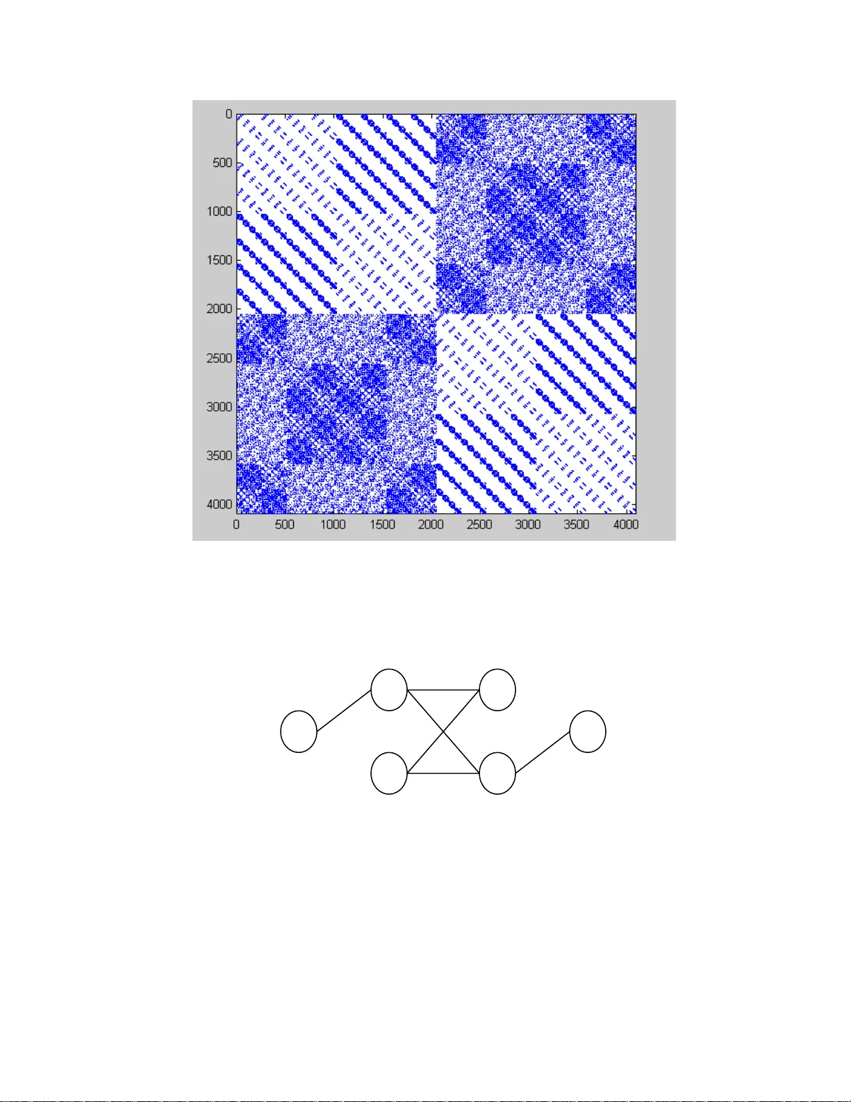
Accepted for publications in In ternational Journal of Wireless Information Networks (IJWIN) On the Search for High-Rate Quasi-Orthogonal Space-Time Block Code Chau Yuen, Yong Liang Guan, Tjeng Thiang Tjung Abstract – A Quasi-Orthogonal Space-Time Block Code (QO-STBC) is attractive because it achieves higher code rate than Orthogonal ST BC and lower decoding com plexity than non- orthogonal STBC. In this paper, we first derive the algebraic stru cture of QO-STBC, then we apply it in a novel graph-based s earch algorithm to find high-rate QO- STBCs with code rates greater than 1. From the four-antenna codes found using this approach, it is found that the maximum code rate is limited to 5/4 with symbolwise diversity level of four, and 4 with symbol wise diversity level of two. The maximum likelihood decoding of these high-rate QO-STBCs can be performed on two separate sub-groups of symbols. The rate-5/4 codes are the firs t known QO-STBCs with code rate greater 1 that has full symbolwise diversity level. Keywords – High code rate, Multiple Input Multip le Ou tput (MIMO), Quasi-Orthogonal Space- Time Block Code (QO-STBC), Transmit diversity. 1. I NTRODUCTION Orthogonal Space-Time Block Code (O-STBC) can provide full transmit diversity with sim ple linear maximum-likelihood (ML) decoding com ple xity. This, however, limits its m aximum 2 achievable code rate to be less than one when the num ber of transmit antennas ex ceeds two [1]. Specifically, for 4 transmit antennas, the m aximu m achievable code rate of O-STBC has been shown to be 3/4. From the information theoretic vi ewpoint [ 2], this implies th at O-STBC suffers a loss of capacity. As a result, Quasi-Orthogonal Space-Time Block Code (QO-STBC), which can achieve a higher code rate than O-STBC at the expense of a slightly higher decoding complexity, has been investigated [3-7]. The ML decoding of QO-STBC can be achieved by jointly detec ting a sub-group of the transmitted symbols, rather th an all the transmitted sym bols, hence QO-STBC leads to a lower decoding complexity than general non-orthogonal STBC. In [6,7], it is shown that QO-STBC for four transmit antennas th at require the jo int detection of only two real symbols for ML de coding has a maximum code rate of 1. This, when compared against the maximum code rate of 3/4 and linear decoding complexity for an O-ST BC for the same number of transmit antennas, suggests that the ma ximum code rate of QO -STBC may exceed 1 if a decoding complexity higher than the joint detection of two re al symbols is permitted. In this paper, we set out to search for such “high-rate QO-ST BC” with code rate greater than one. To our knowledge, this is the first such attempt ever conducted on QO-STBC. The organization of this paper is as fo llows: Section 2 gives the signa l model and derives the unifying algebraic structure of a QO-STBC. Section 3 discusses the modeling of the code search problem, and introduces a novel graph-based algorith m to perform the code search, based on graph theory. Finally Section 4 concludes the paper. 3 2. Q UASI -O RTHOGONAL S PACE -T IME B LOCK C ODE 2.1 STBC Model Suppose that there are N t tansmit antennas, N r receive antennas, and an interval of T symbol periods during which the propagation channel is constant and known to the receiver. The information data sequ ence is segmented into blocks of K complex symbols { x 1 , x 2 , …, x K }, each for transmission using a ST BC. The transmitte d STBC codeword can be written as a T × N t matrix G that governs the transmission over N t antennas and T symbol periods. The code rate of the STBC is defined as K / T . Following the STBC model in [8] with the complex symbol x k expressed as x k = s k + j s K + k , 1 ≤ k ≤ K , the STBC codeword G can be expressed as: 2K 1 () ii i s = = ∑ GA ( 1 ) where the matrices A i are called the “dispersion matrices”, have size T × N t , and are normalised by the power distribution constraint H tr ( ) / ii t TN K = AA [8]. The received signal model for a system with multiple receive an tennas can been shown to be: t N ρ =+ rH s η   ( 2 ) where the normalization t N ρ is to ensure that the SNR ( ρ ) at the receiver is independent of the number of transm it antennas, and RR 1 11 II 11 RR 1 II 2 ,,, rr rr K K NN NN K s s s s + ⎡⎤ ⎡⎤ ⎡ ⎤ ⎢⎥ ⎢⎥ ⎢ ⎥ ⎢⎥ ⎢⎥ ⎢ ⎥ ⎢⎥ ⎢⎥ ⎢ ⎥ == = ⎢⎥ ⎢⎥ ⎢ ⎥ ⎢⎥ ⎢⎥ ⎢ ⎥ ⎢⎥ ⎢⎥ ⎢ ⎥ ⎢⎥ ⎣⎦ ⎣ ⎦ ⎢⎥ ⎣⎦ r η r η rs η r η r η # ##   # 4 11 2 1 1 2 1 12 2 ... ... , ... ... rr r r KK N N KN KN ⎡⎤ ⎢⎥ = ⎢⎥ ⎢⎥ ⎣⎦ hh h h H hh h h ## % # % # AA A A AA A A RI R IR I ,. ii i ii ii i ⎡ ⎤⎡ ⎤ − == ⎢ ⎥⎢ ⎥ ⎣ ⎦⎣ ⎦ AA h h AA h A In (2), r i and η i , where 1 ≤ i ≤ N r , are T × 1 column vectors which cont ain the received signal and zero-mean unit-variance AWGN noise for the i th receive antenna over T symbol periods; H is the equivalent channel matrix, and h i is a N t × 1 column vector that contai ns the Rayleigh flat fading coefficients from the N t transmit antennas to i th receive antenna. The superscripts ( ) R and ( ) I denote the real and imaginary parts respectively of a complex element, vector or m atrix. 2.2 Algebraic Structure of QO-STBC The concept of quasi-orthogonality in QO-ST BC refers to the division of the K transmitted symbols in a QO-STBC codeword into G different groups such that symbols in one group are orthogonal to all symbols in the other groups, while strict orthogonality am ong the sym bols within a group is not required. Orthogonality in this case m eans that, by linear matched filtering at the receiver, the received symbols of the QO-STBC can be de-coupled into G independent groups, and the ML decoding of different groups can be pe rformed separately and in paralle l by jointly detecting only K / G complex symbols within a group [9], instead of jointly detecting all K com plex symbols within a codeword (which is clearly a m ore complex operation). Definition 1 : A quasi-orthogonal design is such that its corresponding H T H (with H as defined in (2)) can be rearranged into a block-diagonal m atrix with non-zero s ub-matrices of size (2 K / G ) 5 × ( 2 K / G ) by a permutation, i.e. P T H T HP is block diagonal, where P T P = I and P has only unit entries. Without loss of generality, throughout this paper, we assume that P = I , where I is an identity matrix of appropriate dimension. It should be noted that, in contrast to Definition 1 , an orthogonal design requires the H T H to be a scaled identity matrix [1] , instead of a block-diagonal m atrix for the quasi-orthogonal design. In order to separate the rece ived signals into G orthogonal groups, a matched filter H T is multiplied to the received signal r  in (2). Let us consider a snapshot of H T H as follows : TT T T 1 TT T T 111 1 1 T TT T T 1 TT T T 1 r r r rrr r r pN p pu qv uN u qN q pN uN qN vN vN v ⎡⎤ ⎢⎥ ⎢⎥ ⎡⎤ ⎢⎥ ⎢⎥ ⎢⎥ = ⎢⎥ ⎢⎥ ⎢⎥ ⎢⎥ ⎣⎦ ⎢⎥ ⎢⎥ ⎣⎦ = hh hhh h hh HH hh hhh h hh #" # " "" " ## # # # # " "" " #" # "" " " AA AA A A AA AA AA A A AA () () () () () () () () () () TT TT TT TT 11 1 1 TT TT TT TT 11 1 1 TT TT 11 RR R R RR R R R NN N N ip p i ip u i ip q i ip v i ii i i NN N N iu p i iu u i iu q i iu v i ii i i NN iq p i iq u i ii == = = == = = == ∑∑ ∑ ∑ ∑∑ ∑ ∑ ∑ hh h h h h h h hh h h h h h h hh h h "" # # # # # # AA AA AA AA AA AA AA AA AA AA () () () () () () TT T T 11 TT TT TT T T 11 1 1 RR R RR R R NN iq q i iq v i ii NN N N iv p i iv u i iv q i iv v i ii i i == == = = ⎡ ⎢ ⎢ ⎢ ⎣ ∑∑ ∑ ∑∑ ∑ ∑ hh h h hh h h h h h h # # "" " " " " AA AA AA AA AA AA ⎤ ⎥ ⎥ ⎥ ⎢ ⎥ ⎢ ⎥ ⎢ ⎥ ⎢ ⎥ ⎢ ⎥ ⎢ ⎥ ⎢ ⎥ ⎦ (3) where 1 ≤ p, q, u, v ≤ 2 K . Assume that the symbols s p and s u are in the same group (hence they are not orthogonal), while the symbols s q and s v are in another group (hen ce they are orthogonal to s p and s u ). We write { p, u } ⊂ G ( p ) and { q, v } ⊄ G ( p ), where G ( p ) represents a set of symbol i ndices that are in the sam e group 6 as symbol with index p , including p ; similarly, { q, v } ⊂ G ( q ) and { p, u } ⊄ G ( q ). In order to achieve orthogonality among the symbols of diffe rent groups, e.g. between sym bols s u and s v , the summation terms included in the boxes in (3) a re required to be zero, hence A u T A v and A v T A u (likewise for A p T A v , A u T A q , A p T A q , etc.) have to be skew-symmetric, i.e. ( A u T A v ) T = – A u T A v , ( A v T A u ) T = – A v T A u and so on. Theorem 1 : For symbols with index u and v to be orthogonal to each other, i.e. A u T A v and A v T A u to be skew-symmetry, the f ollowing Quasi-Orthogonality Constraint (QOC) has to be fulfilled: HH 1 , 2 and ( ) uv v u uv K v u =− ≤ ≤ ∉ AA AA G (4) Proof of Theorem 1 : ( ) () () ( ) () ( ) () ( ) () ( ) () ( ) HH HH RI RI RI RI TT T T RR I I RR II TT TT RI I R RI I R real pa rt: ima g par t: uv v u uuv v v v uu uv u v vu v u uv u v vu v u jj j j =− ⇒+ + = − + + ⎧ += − − ⎪ ⇒ ⎨ ⎪ −= − + ⎩ AA AA AAAA AA AA AA A A AA A A AA A A AA A A (5) Defining () ( ) () ( ) TT RR I I TT RI I R uv u v uv u v ⎧ + ⎪ ⇒ ⎨ ⎪ − ⎩ MA A A A NA A A A   7 then (5) shows that M is skew-symmetry (i.e. M T = – M ) and N is symmetric (i.e. N T = N) . Si nce T uv − ⎡⎤ = ⎢⎥ ⎣⎦ MN NM AA , it is easy to verify that A u T A v is skew-symmetry. Similar conclusion can be shown for A v T A u . Therefore, by restric ting the dispersion matrices A of symbols belong to different groups to satisfy the QOC in (4), orthogonality among the sym bols of different groups can be achieved. Hence Theorem 1 i s p r o v e d . ■ Note that when there is only one re al symbol in a group, the QOC in Theorem 1 becomes the orthogonality constraint for O-STBC pr ovided in [1,14], and the condition () vu ∉ G in (4) is no longer needed as there will be only one real symbol in a grou p for O-STBC. It can be shown that all the disp ersion m atri ces of the QO-STBCs in [3-7] conform to the QOC in (4), hence (4) formulates th e algebraic stru cture of a generic QO-STBC. We will make use of this algebraic structure to search for dispersion matrices tha t form a QO -STBC with the desired code rate in the next section. 3. S EARCH OF H IGH R ATE QO-STBC 3.1 Code Parameters Before performing the code sear ch, we first define the parame ters used for generating the dispersion matrices of a QO-STBC: • Code length : The code length, T , of the QO-STBC is assumed be equal to the num ber of 8 transmit antennas, i.e. T = N t in this paper. So the codeword is a square matrix. • Matrix Entries : The entrie s of the dispersion m atrix are set to be {0, ± 1, ± j }, as commonly adopted in the literature [1,3-7]. • Matrix Rank : The rank of a dispersio n matrix is related to th e symbolwise divers ity of the STBC, e.g. a code with dispersion matr ices of rank 2 can never provide transm it diversity greater than 2. A disp ersion matrix with rank equal to N t is said to achieve the maximal symbolwise diversity [10]. • Matrix Weight : This parameter refers to the number of non-zero entries in every row of a dispersion matrix. • Group : This parameter is as defined in Section 2.2 and Definition 1. For QO-STBC, G is required to be more than 1 (G = 1 gives a fully non-orthogonal STBC). 3.2 Code Search Methodology Our proposed code search methodology works as follows: we first cons truct a set of “seed matrices” as potential QO-STBC dispersion m atrices, and then perform a search among these matrices to look for valid QO-STBC dispersion matrices. In order to increase the chance of finding QO-STBC with rate greater than 1, it is desired to have as many seed matrices as possible. Hence in this paper, we consider seed matrices with comp lex number entries, as well as matrices with bo th weights 1 and 2. The code search procedure can be br oadly formulated into three steps: (a) Generate a series of N matrices (the so called “seed ma trices ”) with desired parameters , e.g. T = N t = 4, rank = 4, weight = 2. 9 (b) From the matrices obtained in Step (a), iden tify and retain those that can be grouped into G groups according to the QOC in (4). (c) From the matrices obtained in Step (b), identify those th at can provide a code rate greater than one, i.e. matrices that give an equivalent channel m atrix of rank > 2 T (relationship between the rank of the equivalent channel matrix and the code rate of a QO-STBC will be explained in the f ollowing part). The above steps are elaborated below. Step (a) Consider the case of T = N t = 4, rank 4 and weight 2. To generate matrices with these parameters, we start with the sixteen 2×2 co mplex Hadamard m atrices with entries {0, ± 1, ± j } shown in Figure 1, a nd use them as the P and Q sub-matrices in the sixteen 4×4 m atrices shown in Figure 2. By doing so, N = 16 3 = 4096 matrices of size 4×4, rank 4 and weight 2 can be generated. Step (b) Group these N = 4096 matrices into G groups based on the QOC in (4). However this is an NP-complete problem because each of the N matrices can be eithe r in one of the G groups, or not in any group at all, so there are ( G +1) N possible combinations. Hence an efficient algorithm is required to expedite this search/grouping process. A novel method based on graph theory is proposed in this paper to acco mplish this task. It will be described in Section 3.3. 10 Step (c) Assume that M dispersion matrices (grouped into G groups) are found in Step (b). The objective of Step (c) is to check the rank, R , of the equivalent channel matrix H (2) form ed by these M dispersion matrices. R represents the number of real sym bols that can be supported by the equivalent channel H . If R < M , it implies that M – R dispersion matrices are linearly dependent on the R independent dispersion matrices. So only R out of the M dispersion m atrices can be used to form a QO-STBC with a resultant code rate of R /(2 T ). On the other hand, R = M is the m aximum achievable value for R . In order to achieve a code rate greater than one, it is required that R > 2 T . 3.3 Graph Modelling and Modified Depth First Search for Implementing Step (b) Now we present an efficient gra ph-based technique to identify th e matrices from those found in Step (a) that can be grouped into G groups according to the QOC in (4). The quasi-orthogonal relationship between the set of N = 4096 matrices can be visualized in Figure 3, which indicates the matrix index u on the x-axis and the m atrix index v on the y-axis for all 1 ≤ u , v ≤ N , and marks the ( u , v ) point as a dark pixel if the corresponding ( A u , A v ) matrices satisfy the QOC. A close examination of Figure 3 shows that every matrix sa tisfies th e QOC with another 56 matrices. So if we view Figure 3 as a matrix, it is a sparse ma trix in which only 56/4096 = 1.37% of the matrix entries are non-zero (this is m uch less than the ge neral definition of sparse matrix which require non-zero entries to be less than 10%) [11]. One of the efficient representations of sparse matrix is the graph model. This suggests that the code search/grouping problem in Step (b) can be so lved with the help of graph theory and graph- 11 based algorithms. Specifically, we model the N matrices found in Step (a) as a series of N nodes in a graph. For every pair of matri ces that satisfy the QOC in (4), their nodes will be connected by a unidirectional link. Hence a graph with nodes re presenting possible QO-ST BC dispersion matrices, and connected by links denoting conformance to the QOC between the connected nodes, will be formed. A simple example of such a graph is shown in Figure 4, where the m atrix A 1 is assumed to satisfy QOC with matrices A 2 , A 4 and A 5 ; while the matrix A 3 is assumed to satisf y QOC with matrices A 2 and A 4 ; and so on. The graph example in Figure 4 suggests that A 1 , A 2 , A 3 and A 4 can form a QO-STBC with dispersion matrices A 1 and A 3 in a group, and dispersion matrices A 2 and A 4 in another group. These two groups of dispersion matrices are orthogonal to each other, because A 1 and A 3 establish the QOC link with A 2 and A 4 , and vice versa. In a QO-STBC, si nce the dispersion matrices in any group must satisfy the QOC with the dispersion matrices in all other groups, in our proposed graph model we can always find links that connect ever y matrix in a group to every matrix in another group. In short, a QO-STBC forms a fully connected graph with nodes representing its dispersion matrices and links connecting dispersion matrices of different groups. By exploiting this property, if we randomly pick a matrix node in this graph as th e starting point to pe rform a “spanning tree algorithm” [12], we will be able to id entify the quasi-orthogona l grouping of the N matrice s obtained from Step (a). Depth First Search (DFS) [12] is an algorithm in graph theory that provides a sy stematic way to visit all the nodes in a graph from any starti ng node and form a spanning tree. The pseudo codes of DFS algorithm are given in Appendix A. In order to solve the dispersion matrix grouping problem in Step (b), we propose to extend the DFS algorithm to a modified DFS (MDFS) 12 algorithm. The pseudo codes of the proposed MDFS algorithm are given in A ppendix B. Essential differences between the DFS and MD FS algorithms are listed below: • In MDFS, every node can be visited more than once. In D FS, every node can only be visited once. • In MDFS, there is an assignment of group to the nodes visited. There is no such assignment in DFS. • In MDFS, there is an additional requirement that every visited node must be connected with its ancestors of different groups. There is no such requirement in DFS. Based on the graph example in Figure 4, th e trees constructed by DFS and MDFS with G = 2 are shown in Figure 5(a) and (b) respectively. Every branch of the tree constructed by MDFS constitutes a possible solution for the dispersion matrices of a QO-STBC. For example in Figure 5(b), A 1 - A 2 - A 3 - A 4 and A 1 - A 4 - A 6 and A 1 - A 5 are possible solutions, but A 1 - A 4 - A 3 - A 2 is not as it is merely a permutation of the first branch. On the other hand, the A 1 - A 2 - A 3 - A 4 - A 6 branch in the DFS tree in Figure 5(a) is not a valid QO- STBC solution because although A 6 has a QOC link with A 4 (which is in group 2), it does not have a QOC link with its ancestor node A 2 (which is also in group 2), hence A 6 cannot be added as group 1 node and cannot form a QO-STBC together with A 2 and A 4 . This explains why the basic DFS algorithm cannot be used for solving the code search problem described in Step (b). Back to Figure 5(b), since we want a QO-STBC w ith as high code rate as possible, only the A 1 - A 2 - A 3 - A 4 branch is considered as it gives a QO- STBC with the largest number of dispersion matrices. The resultan t QO-STBC has a group of dispersion matrices consisting of A 1 & A 3 , and another group of dispersi on matrices consisting of A 2 & A 4 . So a total of M = 4 dispersion matrices, 13 divided into two orthogonal gr oups, are found. Hence the proposed MDFS algorithm can be used for solving the code search pr oblem discussed in Step (b). 3.4 Code Search Results Using the proposed MDFS algorithm with G = 2 on the set of N = 4096 matrices with rank 4 and weight 2 described earlier, we are able to find a few set of solutions each with M = 16 matrices grouped into two orthogonal groups. Each of these solution sets each form an equivalent channel matrix with a rank of R = 10, resulting in a QO-STBC for four transmit antennas with code length T = 4, code rate = R /2 T = 5/4 and maxim al symbolwise diversity. One of such solution sets is given in Appendix C and we will use it to discuss the relationship between equivalent channel matrix rank and code rate. From the matrices A 1 to A 16 shown in Appendix C, one can easily verify that the matrices A 1 to A 8 satisfy the QOC with the matric es A 9 to A 16 . In other words, they may form a QO-STBC with two quasi-orthogonal groups. However, although A 1 to A 16 are 16 different matrices, the equivalent channel matrix formed by them has a rank of only 10, instead of 16. In ot her words, only 10 out of these 16 matrices ( A 1 to A 5 and A 9 to A 13 ) are linearly independent and can be used as dispersion matrices to carry inform ation sym bols, while the other 6 matrices ( A 6 to A 8 and A 14 to A 16 ) are linearly dependent on the earlier 10 matrices and hence cannot be used to carry any new information symbol. Since every dispersion m atrix ca rry a real information symbol and the m atrices in Appendix C have length 4, the resultant QO-STBC has a code rate of 10/2/4 = 5/4. Table I summarizes the results of our code resear ch using various code parameters. It shows that rate-5/4 QO-STBCs exist with symbolwise di versity level = 4 and group = 2, while rate-4 QO- 14 STBCs exist with symbolwise diversity level = 2 and group = 2. One of th e solution sets found for the rate-4 QO-STBC is given in Appendix D. Other interesting obs ervations include: • All QO-STBCs with code rate greater than one (shaded rows in Table I) have dispersion matrices separated into 2 groups and weights greater than 1. • To achieve a higher code rate from 5/4 to 4, the rank of the dispersion matrices (hence the symbolwise diversity level) is reduced from 4 to 2, i.e. full transmit diversity can no longer be achieved. • The rate-4 diversity -2 length-4 QO-STBC found turns out to be equivalent to the rate-4 diversity-2 length-2 non-orthogona l STBCs [13, 15], and both of them have the same decoding complexity. Nonetheless its existenc e, when compared with the rate-5/4 code found, illustrates the tradeoff between code rate, diversity of high-rate QO-STBC. 4. C ONCLUSION In this paper, the algebraic c onstraint of the dispersion matric es of a QO-STBC is derived and applied in a graph-based approach to provide a computer search f or QO-STBC with code rate greater than one. Due to the high complexity o f th is code search problem , an efficient Modified Depth First Search (MDFS) algorithm, which is extended from the Depth First Search algorithm well known in graph theory, is pro posed to facilitate the code search. For 4 transmit antennas, a few QO-STBCs with rates 5/4 and 4 are found. A trade-off between the code rate and the symbolwise transmit diversity level is observed in these high-rate QO-STBCs, as the rate-5/4 codes have symbolwise diversity of 4 while the rate-4 co des have symbolwise divers ity of 2. All the high- 15 rate QO-STBCs obtained are also found to have dispersion matrices separable into 2 quasi- orthogonal groups and the “weights” of these dispersion matrices are f ound to be two, i.e. there are two non-zero entries in every row of the dispersion matrices. To our knowledge, the rate-5/4 codes are the first known non-trivial QO-STBCs with code rate > 1. AKNOWLEDGEMENTS The authors would like to thank Hwor Sh en Chong and Chee Muah Lim from Nanyang Technological University (Singapore) in assisting in part of this work. The authors would also like to thank the editor Dr Olav Tirkkonen and th e anonymous reviewer for many constructive suggestions that help improve the quality of this paper. REFERENCES [1] V. Tarokh, H. Jafarkhani, and A. R. Cald erbank, “Space-time block codes from orthogonal designs”, IEEE Trans. on Information Theory, vol. 45, pp. 1456-1467, Jul. 1999. [2] S. Sandhu and A. Paulraj, “Space-time block codes: a capacity perspective”, IEEE Communications Letters , vol. 4, pp. 384-386, Dec. 2000. [3] H. Jafarkhani, “A quasi-ort hogonal space-time block code”, IEEE Trans. on Communications, vol. 49, pp. 1-4, Jan. 2001. 16 [4] C. B. Papadias and G. J. Foschini, “Cap acity-approaching space-time codes for systems employing four transmitter antenn as”, IEEE Trans. on Information Theory , vol. 49, pp. 726- 733, Mar. 2003. [5] O. Tirkkonen, A. Boariu, and A. Hottinen, “Min imal non-orthogonality rate 1 space-tim e block code for 3+ tx antennas”, IEEE ISSSTA 2000, vol. 2, pp. 429-432. [6] C. Yuen, Y. L. Guan, and T. T. Tjhung, “Construction of Quasi-Orthogonal STBC with Minimum Decoding Complexity”. IEEE ISIT 2004 , pp. 309. Also accepted for publica tion in IEEE Trans. Wireless Comms . [7] C. Yuen, Y. L. Guan, and T. T. Tjhung, “A lgebraic relationship between quasi-orthogonal STBC with minimum decoding complexity an d amicable orthogonal design”, su bmitted to IEEE ICC 2006 . [8] B. Hassibi and B. M. Hochwald, “High-rate codes that are linear in space and time”, IEEE Trans. on Information Theory , vol. 48, pp. 1804 –1824, Jul. 2002. [9] C. Yuen, Y. L. Guan, and T. T. Tjhung, “D ecoding of quasi-orthogonal space-time block code with noise whitening”, IEEE PIMRC 2003 , pp. 2166-2170. [10] O. Tirkkonen, “Maximal sym bolwise diversity in non-orthogonal space-time block codes”, IEEE ISIT 2001 , pp.197. [11] U. Schendel, Sparse Matrices, numerical aspects wi th applications for scientists and engineers , John Wiley & Sons, 1989. [12] S. Sahni, Data Structures, Algorithms, and Applications in C++ , McGraw-Hill, 1998. [13] A. Hottinen, O. Tirkkonen, X. W ichman, “Multiantenna techniques for 3G and beyond”, John Wiley & Sons, 2003. 17 [14] O. Tirkkonen and A. Hottinen, “Square-m atri x embeddable space-time block codes for complex signal constellations”, IEEE Trans. on Information Theory , vol. 48, pp. 384-395, Feb. 2002. [15] C. Yuen, Y. L. Guan, and T. T. Tjhung, “New high-rate STBC with good dispersion property”, IEEE PIMRC 2005 . 18 Table Table I Code search results found using proposed MDFS algorithm Parameters Matrix Rank (symbolwise diversity) Matrix Weight Group Max. Code Rate 4 1 4 1 4 1 2 1 4 2 2 5/4 2 2 8 1 2 2 2 4 19 Figures 11 11 1 1 1 1 1 1 1 1 11 11 11 11 1 1 1 1 11 1 1 11 1 1 11 1 1 11 1 1 j j j j jj jj jj j j jj j j jj j j j jjj −− ⎡⎤ ⎡⎤ ⎡⎤ ⎡⎤ ⎢⎥ ⎢⎥ ⎢⎥ ⎢⎥ −− ⎣⎦ ⎣⎦ ⎣⎦ ⎣⎦ −− ⎡⎤ ⎡⎤ ⎡ ⎤ ⎡ ⎤ ⎢⎥ ⎢⎥ ⎢ ⎥ ⎢ ⎥ −− ⎣⎦ ⎣⎦ ⎣ ⎦ ⎣ ⎦ −− ⎡ ⎤ ⎡⎤ ⎡ ⎤ ⎡⎤ ⎢ ⎥ ⎢⎥ ⎢ ⎥ ⎢⎥ −− ⎣ ⎦ ⎣⎦ ⎣ ⎦ ⎣⎦ −− ⎡⎤ ⎡ ⎤ ⎡ ⎤ ⎡ ⎤ ⎢⎥ ⎢ ⎥ ⎢ ⎥ ⎢ ⎥ − −− − ⎣⎦ ⎣ ⎦ ⎣ ⎦ ⎣ ⎦ Figure 1 Complex Hadamard matrices of weight two jj jj j j jj jj jj j j jj ⎡⎤ ⎡ ⎤ ⎡ ⎤ ⎡ ⎤ ⎢⎥ ⎢ ⎥ ⎢ ⎥ ⎢ ⎥ −− ⎣⎦ ⎣ ⎦ ⎣ ⎦ ⎣ ⎦ ⎡⎤ ⎡ ⎤ ⎡ ⎤ ⎡ ⎤ ⎢⎥ ⎢ ⎥ ⎢ ⎥ ⎢ ⎥ −− ⎣⎦ ⎣ ⎦ ⎣ ⎦ ⎣ ⎦ ⎡⎤ ⎡ ⎤ ⎡ ⎤ ⎡ ⎤ ⎢⎥ ⎢ ⎥ ⎢ ⎥ ⎢ ⎥ −− ⎣⎦ ⎣ ⎦ ⎣ ⎦ ⎣ ⎦ ⎡⎤ ⎡ ⎤ ⎡ ⎤ ⎡ ⎤ ⎢⎥ ⎢ ⎥ ⎢ ⎥ ⎢ ⎥ −− ⎣⎦ ⎣ ⎦ ⎣ ⎦ ⎣ ⎦ P0 P 0 P 0 P 0 0Q 0 Q 0 Q 0 Q P0 P 0 P 0 P 0 0Q 0 Q 0 Q 0 Q 0P 0 P 0 P 0 P Q0 Q0 Q0 Q0 0P 0 P 0 P 0 P Q0 Q0 Q0 Q0 Figure 2 Patterns to generate matric es of rank four and weight two 20 Figure 3 QOC link connection between 4×4 matrices formed in Step (a) Figure 4 Example of a graph A 1 A 2 A 3 A 4 A 5 A 6 21 (a) DFS tree (b) MDFS tree Figure 5 Trees generated by DFS and MDFS algorithms A 1 A 2 A 3 A 4 A 5 A 6 A 1 A 2 A 3 A 4 A 4 A 3 A 2 A 6 A 5 Group 1 node Group 2 node 22 APPENDIX A: Depth First Search (DFS) Algorithm Input: Graph, number of nodes in graph ( N ) Output: a spanning tree T with every node visited only once Begin Pick a node n , n ≤ N as starting point; Assign node n as the root of tree T , i.e. T = T ∪ { n }; DFS( n , T ); End Procedure DFS( n , T ) Begin for ( v ∈ {neighbor of n }) if ( v ∉ T ) % i.e. v not in the tree T Add node v to the tree T with n as parent, i.e. T = T ∪ { v }; DFS( v , T ); end end End 23 APPENDIX B: Modified Depth Fi rst Search (MDFS) Algorithm Input: Graph, number of nodes in graph ( N ), number of groups required ( G ) Output: a tree T with every branch as a valid solution Begin Pick a node n , n ≤ N as starting point; Assign node n to Group 1, i.e. g ( n ) =1; Assign node n as the root of tree T , i.e. T = T ∪ { n }; MDFS( n , T , g ); End Procedure MDFS( n , T , g ) Begin for ( v ∈ {neighbor of n }) if ( v ∉ {ancestor of n }) Assume that node v is in Group p where p = g ( n )+1 if g ( n )+1 ≤ G , = 1 if g (n)+1 > G ; if ( v possesses a link with all ancestors of n with different groups, i.e. g(ancestor of n) ≠ p ) Assign node v to Group p , i.e. g ( v ) = p ; Add node v to the tree T with n as parent, i.e. T = T ∪ { v }; MDFS( v , T , g ); end end end END 24 APPENDIX C: Matrices found by MDFS using G = 2, T = N t = 4, rank = 4, weight = 2 Group 1 1 1100 11 0 0 0011 001 1 ⎡⎤ ⎢⎥ − ⎢⎥ = ⎢⎥ ⎢⎥ − ⎣⎦ A , 2 11 0 0 11 0 0 00 1 1 00 1 1 ⎡⎤ ⎢⎥ − ⎢⎥ = ⎢⎥ − − ⎢⎥ − ⎣⎦ A , 3 11 0 0 11 0 0 00 00 jj jj ⎡ ⎤ ⎢ ⎥ − ⎢ ⎥ = ⎢ ⎥ ⎢ ⎥ − ⎣ ⎦ A , 4 11 0 0 11 0 0 00 00 jj jj ⎡⎤ ⎢⎥ − ⎢⎥ = ⎢⎥ − ⎢⎥ ⎣⎦ A , 5 11 0 0 11 0 0 00 00 jj jj ⎡⎤ ⎢⎥ − ⎢⎥ = ⎢⎥ − ⎢⎥ ⎣⎦ A , 6 11 0 0 11 0 0 00 00 jj jj ⎡ ⎤ ⎢ ⎥ − ⎢ ⎥ = ⎢ ⎥ − − ⎢ ⎥ − ⎣ ⎦ A , 7 11 0 0 11 0 0 00 00 jj jj ⎡⎤ ⎢⎥ − ⎢⎥ = ⎢⎥ − ⎢⎥ −− ⎣⎦ A , 8 11 0 0 11 0 0 00 00 jj jj ⎡⎤ ⎢⎥ − ⎢⎥ = ⎢⎥ − ⎢⎥ − − ⎣⎦ A . Group 2 9 11 0 0 1100 00 1 1 0011 − ⎡⎤ ⎢⎥ ⎢⎥ = ⎢⎥ − ⎢⎥ ⎣⎦ A , 10 11 0 0 110 0 001 1 00 1 1 − ⎡⎤ ⎢⎥ ⎢⎥ = ⎢⎥ − ⎢⎥ − − ⎣⎦ A , 11 00 00 00 1 1 00 1 1 jj jj ⎡ ⎤ ⎢ ⎥ − ⎢ ⎥ = ⎢ ⎥ − ⎢ ⎥ ⎣ ⎦ A , 12 00 00 00 1 1 00 1 1 jj jj ⎡⎤ ⎢⎥ − ⎢⎥ = ⎢⎥ − ⎢⎥ ⎣⎦ A , 13 00 00 00 1 1 00 1 1 jj jj − ⎡⎤ ⎢⎥ ⎢⎥ = ⎢⎥ − ⎢⎥ ⎣⎦ A , 14 00 00 00 1 1 00 1 1 jj jj ⎡ ⎤ ⎢ ⎥ − ⎢ ⎥ = ⎢ ⎥ − ⎢ ⎥ − − ⎣ ⎦ A , 15 00 00 00 1 1 00 1 1 jj jj ⎡⎤ ⎢⎥ − ⎢⎥ = ⎢⎥ − ⎢⎥ −− ⎣⎦ A , 16 00 00 00 1 1 00 1 1 jj jj − ⎡⎤ ⎢⎥ ⎢⎥ = ⎢⎥ − ⎢⎥ − − ⎣⎦ A . 25 APPENDIX D: Matrices found by MDFS using G = 2, T = N t = 4, rank = 2, weight = 2 Group 1 1 1100 1100 0011 0011 A ⎡⎤ ⎢⎥ ⎢⎥ ⎢⎥ = ⎢⎥ ⎢⎥ ⎢⎥ ⎣⎦ 2 00 00 00 00 jj jj jj jj A ⎡⎤ ⎢⎥ ⎢⎥ ⎢⎥ = ⎢⎥ ⎢⎥ ⎢⎥ ⎣⎦ 3 0011 0011 1100 1100 A ⎡ ⎤ ⎢ ⎥ ⎢ ⎥ ⎢ ⎥ = ⎢ ⎥ ⎢ ⎥ ⎢ ⎥ ⎣ ⎦ 4 00 00 00 00 jj jj jj jj A ⎡⎤ ⎢⎥ ⎢⎥ ⎢⎥ = ⎢⎥ ⎢⎥ ⎢⎥ ⎣⎦ 5 11 0 0 11 0 0 00 1 1 00 1 1 A ⎡⎤ ⎢⎥ ⎢⎥ ⎢⎥ = ⎢⎥ −− ⎢⎥ ⎢⎥ −− ⎣⎦ 6 00 00 00 00 jj jj jj jj A ⎡⎤ ⎢⎥ ⎢⎥ ⎢⎥ = ⎢⎥ −− ⎢⎥ ⎢⎥ −− ⎣⎦ 7 00 1 1 00 1 1 11 0 0 11 0 0 A ⎡ ⎤ ⎢ ⎥ ⎢ ⎥ ⎢ ⎥ = ⎢ ⎥ −− ⎢ ⎥ ⎢ ⎥ −− ⎣ ⎦ 8 00 00 00 00 jj jj jj jj A ⎡⎤ ⎢⎥ ⎢⎥ ⎢⎥ = ⎢⎥ −− ⎢⎥ ⎢⎥ −− ⎣⎦ 9 11 0 0 11 0 0 00 1 1 00 1 1 A ⎡⎤ − ⎢⎥ ⎢⎥ − ⎢⎥ = ⎢⎥ − ⎢⎥ ⎢⎥ − ⎣⎦ 10 00 00 00 00 jj jj jj jj A ⎡ ⎤ − ⎢ ⎥ ⎢ ⎥ − ⎢ ⎥ = ⎢ ⎥ − ⎢ ⎥ ⎢ ⎥ − ⎣ ⎦ 11 00 1 1 00 1 1 11 0 0 11 0 0 A ⎡ ⎤ − ⎢ ⎥ ⎢ ⎥ − ⎢ ⎥ = ⎢ ⎥ − ⎢ ⎥ ⎢ ⎥ − ⎣ ⎦ 12 00 00 00 00 jj jj jj jj A ⎡⎤ − ⎢⎥ ⎢⎥ − ⎢⎥ = ⎢⎥ − ⎢⎥ ⎢⎥ − ⎣⎦ 13 11 0 0 11 0 0 00 1 1 00 1 1 A ⎡⎤ − ⎢⎥ ⎢⎥ − ⎢⎥ = ⎢⎥ − ⎢⎥ ⎢⎥ − ⎣⎦ 14 00 00 00 00 jj jj jj jj A ⎡ ⎤ − ⎢ ⎥ ⎢ ⎥ − ⎢ ⎥ = ⎢ ⎥ − ⎢ ⎥ ⎢ ⎥ − ⎣ ⎦ 15 001 1 001 1 11 0 0 11 0 0 A ⎡ ⎤ − ⎢ ⎥ ⎢ ⎥ − ⎢ ⎥ = ⎢ ⎥ − ⎢ ⎥ ⎢ ⎥ − ⎣ ⎦ 16 00 00 00 00 jj jj jj jj A ⎡⎤ − ⎢⎥ ⎢⎥ − ⎢⎥ = ⎢⎥ − ⎢⎥ ⎢⎥ − ⎣⎦ Group 2 17 11 0 0 11 0 0 00 1 1 001 1 A ⎡⎤ − ⎢⎥ ⎢⎥ − ⎢⎥ = ⎢⎥ − ⎢⎥ ⎢⎥ − ⎣⎦ 18 00 00 00 00 jj jj jj jj A ⎡⎤ − ⎢⎥ ⎢⎥ − ⎢⎥ = ⎢⎥ − ⎢⎥ ⎢⎥ − ⎣⎦ 19 001 1 00 1 1 11 0 0 11 0 0 A ⎡ ⎤ − ⎢ ⎥ ⎢ ⎥ − ⎢ ⎥ = ⎢ ⎥ − ⎢ ⎥ ⎢ ⎥ − ⎣ ⎦ 20 00 00 00 00 jj jj jj jj A ⎡⎤ − ⎢⎥ ⎢⎥ − ⎢⎥ = ⎢⎥ − ⎢⎥ ⎢⎥ − ⎣⎦ 21 11 00 1100 00 11 0011 A ⎡⎤ −− ⎢⎥ ⎢⎥ ⎢⎥ = ⎢⎥ −− ⎢⎥ ⎢⎥ ⎣⎦ 22 00 00 00 00 jj jj jj jj A ⎡⎤ −− ⎢⎥ ⎢⎥ ⎢⎥ = ⎢⎥ −− ⎢⎥ ⎢⎥ ⎣⎦ 23 00 11 0011 1100 11 00 A ⎡ ⎤ −− ⎢ ⎥ ⎢ ⎥ ⎢ ⎥ = ⎢ ⎥ ⎢ ⎥ ⎢ ⎥ −− ⎣ ⎦ 24 00 00 00 00 jj jj jj jj A ⎡⎤ −− ⎢⎥ ⎢⎥ ⎢⎥ = ⎢⎥ ⎢⎥ ⎢⎥ −− ⎣⎦ 25 11 0 0 11 0 0 00 1 1 001 1 A ⎡⎤ − ⎢⎥ ⎢⎥ − ⎢⎥ = ⎢⎥ − ⎢⎥ ⎢⎥ − ⎣⎦ 26 00 00 00 00 jj jj jj jj A ⎡⎤ − ⎢⎥ ⎢⎥ − ⎢⎥ = ⎢⎥ − ⎢⎥ ⎢⎥ − ⎣⎦ 27 001 1 00 1 1 11 0 0 11 0 0 A ⎡ ⎤ − ⎢ ⎥ ⎢ ⎥ − ⎢ ⎥ = ⎢ ⎥ − ⎢ ⎥ ⎢ ⎥ − ⎣ ⎦ 28 00 00 00 00 jj jj jj jj A ⎡⎤ − ⎢⎥ ⎢⎥ − ⎢⎥ = ⎢⎥ − ⎢⎥ ⎢⎥ − ⎣⎦ 25 1100 11 00 00 11 0011 A ⎡⎤ ⎢⎥ ⎢⎥ −− ⎢⎥ = ⎢⎥ −− ⎢⎥ ⎢⎥ ⎣⎦ 26 00 00 00 00 jj jj jj jj A ⎡⎤ ⎢⎥ ⎢⎥ −− ⎢⎥ = ⎢⎥ −− ⎢⎥ ⎢⎥ ⎣⎦ 27 0011 00 11 1100 11 00 A ⎡ ⎤ ⎢ ⎥ ⎢ ⎥ −− ⎢ ⎥ = ⎢ ⎥ ⎢ ⎥ ⎢ ⎥ −− ⎣ ⎦ 28 00 00 00 00 jj jj jj jj A ⎡⎤ ⎢⎥ ⎢⎥ −− ⎢⎥ = ⎢⎥ ⎢⎥ ⎢⎥ −− ⎣⎦