Manifold Learning: The Price of Normalization

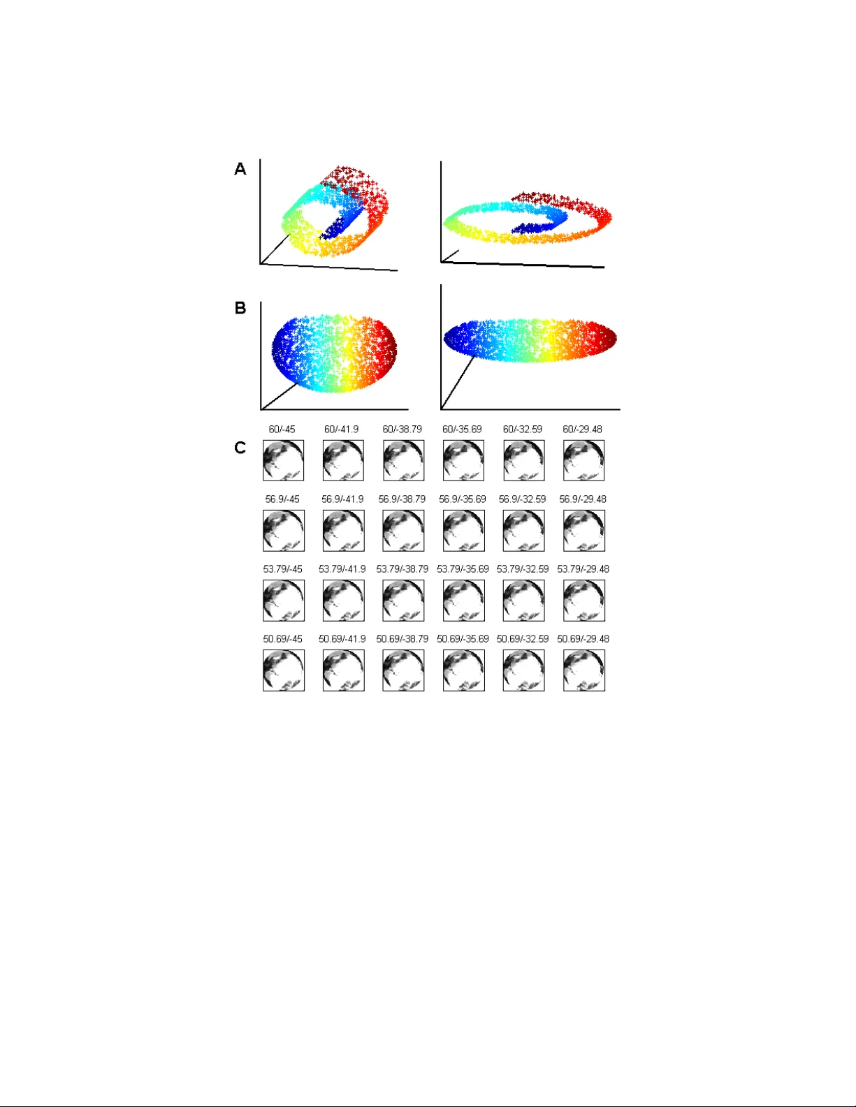
Journal of Machine Learning Researc h ?? (??) ?? Submitted ??; Published ?? Manifold Learning: The Price of Normalization Y air Goldb erg y air go@cc.huji.ac.il Dep artment of Statistics The Hebr ew University, 91905 Jerusalem, Isr ael Alon Zak ai alonzaka@pob.huji.ac.il Inter disciplinary Center for Neur al Computation The Hebr ew University, 91905 Jerusalem, Isr ael Dan Kushnir dan.kushnir@weizmann.a c.il Dep artment of Computer Scienc e and Applie d Mathematics The Weizmann Institute of Scienc e, 76100 R ehovot, Isr ael Y a’aco v Ritov y aa cov.rito v@huji.ac.il Dep artment of Statistics The Hebr ew University, 91905 Jerusalem, Isr ael Editor: ?? Abstract W e analyze the p erformance of a class of manifold-learning algorithms that find their output b y minimizing a quadratic form under some normalization constraints. This class consists of Lo cally Linear Em b edding (LLE), Laplacian Eigenmap, Lo cal T angen t Space Alignment (L TSA), Hessian Eigenmaps (HLLE), and Diffusion maps. W e presen t and pro ve conditions on the manifold that are necessary for the success of the algorithms. Both the finite sample case and the limit case are analyzed. W e show that there are simple manifolds in which the necessary conditions are violated, and hence the algorithms cannot reco ver the underlying manifolds. Finally , we presen t numerical results that demonstrate our claims. Keyw ords: dimensionalit y reduction, manifold learning, Laplacian eigenmap, diffusion maps, lo cally linear em b edding, lo cal tangen t space alignment,hessian eigenmap 1. In tro duction Man y seemingly complex systems describ ed by high-dimensional data sets are in fact go v- erned by a surprisingly low num b er of parameters. Rev ealing the low-dimensional repre- sen tation of such high-dimensional data sets not only leads to a more compact description of the data, but also enhances our understanding of the system. Dimension-reducing algo- rithms attempt to simplify the system’s representation without losing significant structural information. V arious dimension-reduction algorithms were dev elop ed recently to p erform em b eddings for manifold-based data sets. These include the following algorithms: Lo cally Linear Embedding (LLE, Ro weis and Saul, 2000), Isomap (T enen baum et al., 2000), Lapla- cian Eigenmaps (LEM, Belkin and Niyogi, 2003), Local T angen t Space Alignment (L TSA, c  ?? ??. Zhang and Zha, 2004), Hessian Eigenmap (HLLE, Donoho and Grimes, 2004), Semi-definite Em b edding (SDE, W ein b erger and Saul, 2006) and Diffusion Maps (DFM, Coifman and La- fon, 2006). These manifold-learning algorithms compute an embedding for some given input. It is assumed that this input lies on a low-dimensional manifold, em b edded in some high- dimensional space. Here a manifold is defined as a top ological space that is locally equiv alent to a Euclidean space. It is further assumed that the manifold is the image of a low- dimensional domain. In particular, the input points are the image of a sample taken from the domain. The goal of the manifold-learning algorithms is to recov er the original domain structure, up to some sc aling and rotation. The non-linearity of these algorithms allows them to reveal the domain structure ev en when the manifold is not linearly embedded. The cen tral question that arises when considering the output of a manifold-learning algorithm is, whether the algorithm rev eals the underlying low-dimensional structu re of the manifold. The answ er to this question is not simple. First, one should define what “rev ealing the underlying low er-dimensional description of the manifold” actually means. Ideally , one could measure the degree of similarit y b etw een the output and the original sample. Ho wev er, the original low-dimensional data represen tation is usually unkno wn. Nev ertheless, if the lo w-dimensional structure of the data is kno wn in adv ance, one would exp ect it to b e approximated by the dimension-reducing algorithm, at least up to some rotation, translation, and global scaling factor. F urthermore, it w ould b e reasonable to exp ect the algorithm to succeed in recov ering the original sample’s structure asymptotically , namely , when the num b er of input p oints tends to infinit y . Finally , one would hope that the algorithm would b e robust in the presence of noise. Previous pap ers ha ve addressed the cen tral question p osed earlier. Zhang and Zha (2004) presen ted some b ounds on the lo cal-neighborho o ds’ error-estimation for L TSA. How ever, their analysis sa ys nothing ab out the global embedding. Huo and Smith (2006) prov ed that, asymptotically , L TSA recov ers the original sample up to an affine transformation. They assume in their analysis that the lev el of noise tends to zero when the num b er of input p oin ts tends to infinity . Bernstein et al. (2000.) prov ed that, asymptotically , the embedding given b y the Isomap algorithm (T enenbaum et al., 2000) reco vers the geodesic distances b et ween p oin ts on the manifold. In this paper w e dev elop theoretical results regarding the p erformance of a class of manifold-learning algorithms, whic h includes the following fiv e algorithms: Locally Linear Em b edding (LLE), Laplacian Eigenmap (LEM), Lo cal T angen t Space Alignmen t (L TSA), Hessian Eigenmaps (HLLE), and Diffusion maps (DFM). W e refer to this class of algorithms as the normalized-output algorithms. The normalized- output algorithms share a common scheme for recov ering the domain structure of the input data set. This sc heme is constructed in three steps. In the first step, the lo cal neigh b or- ho o d of each p oint is found. In the second step, a description of these neighborho o ds is computed. In the third step, a low-dimensional output is computed by solving some con vex optimization problem under some normalization constrain ts. A detailed description of the algorithms is given in Section 2. In Section 3 we discuss informally the criteria for determining the success of manifold- learning algorithms. W e sho w that one should not exp ect the normalized-output algo- rithms to reco ver geo desic distances or lo cal structures. A more reasonable criterion for 2 The Price of Normaliza tion success is a high degree of similarity b et ween the output of the algorithms and the original sample, up to some affine transformation; the definition of similarity will b e discussed later. W e demonstrate that under certain circumstances, this high degree of similarity do es not o ccur. In Section 4 w e find necessary conditions for the successful p erformance of LEM and DFM on the t wo-dimensional grid. This section serves as an explanatory in tro duction to the more general analysis that app ears in Section 5. Some of the ideas that form the basis of the analysis in Section 4 w ere discussed indep endently by b oth Gerber et al. (2007) and ourselv es (Goldb erg et al., 2007). Section 5 finds necessary conditions for the successful p er- formance of all the normalized-output algorithms on general tw o-dimensional manifolds. In Section 6 we discuss the p erformance of the algorithms in the asymptotic case. Concluding remarks appear in Section 7. The detailed proofs app ear in the App endix. Our pap er has tw o main results. First, we giv e well-defined necessary conditions for the successful p erformance of the normalized-output algorithms. Second, we show that there exist simple manifolds that do not fulfill the necessary conditions for the success of the algorithms. F or these manifolds, the normalized-output algorithms fail to generate output that reco vers the structure of the original sample. W e sho w that these results hold asymptotically for LEM and DFM. Moreo ver, when noise, even of small v ariance, is in tro duced, LLE, L TSA, and HLLE will fail asymptotically on some manifolds. Throughout the paper, w e present numerical results that demonstrate our claims. 2. Description of Output-normalized Algorithms In this section we describ e in short the normalized-output algorithms. The presentation of these algorithms is not in the form presen ted by the resp ectiv e authors. The form used in this pap er emphasizes the similarities b etw een the algorithms and is b etter-suited for further deriv ations. In App endix A.1 w e show the equiv alence of our represen tation of the algorithms and the represen tations that appear in the original pap ers. Let X = [ x 1 , . . . , x N ] 0 , x i ∈ R D b e the input data where D is the dimension of the am bient space and N is the size of the sample. The normalized-output algorithms attempt to reco v er the underlying structure of the input data X in three steps. In the first step, the normalized-output algorithms assign neighbors to each input p oint x i based on the Euclidean distances in the high-dimensional space 1 . This can b e done, for example, by choosing all the input p oin ts in an r -ball around x i or alternatively by c ho osing x i ’s K -nearest-neigh b ors. The neigh b orho o d of x i is giv en by the matrix X i = [ x i , x i, 1 , . . . , x i,K ] 0 where x i,j : j = 1 , . . . , K are the neigh b ors of x i . Note that K = K ( i ) can b e a function of i , the index of the neighborho o d, yet w e omit this index to simplify the notation. F or eac h neigh b orho o d, w e define the radius of the neighborho o d as r ( i ) = max j,k ∈{ 0 ,...,K } k x i,j − x i,k k (1) where we define x i, 0 = x i . Finally , we assume throughout this pap er that the neigh b orho o d graph is connected. 1. The neighborho o ds are not mentioned explicitly b y Coifman and Lafon (2006). How ever, since a sparse optimization problem is considered, it is assumed implicitly that neighborho o ds are defined (see Sec. 2.7 therein). 3 In the second step, the normalized-output algorithms compute a description of the lo cal neigh b orho o ds that w ere found in the previous step. The description of the i -th neigh b or- ho o d is given by some weigh t matrix W i . The matrices W i for the differen t algorithms are presen ted. • LEM and DFM: W i is a K × ( K + 1) matrix, W i =        w 1 / 2 i, 1 − w 1 / 2 i, 1 0 · · · 0 w 1 / 2 i, 2 0 − w 1 / 2 i, 2 . . . . . . . . . . . . . . . . . . 0 w 1 / 2 i,K 0 · · · 0 − w 1 / 2 i,K        . F or LEM w i,j = 1 is a natural c hoice, yet it is also possible to define the w eigh ts as ˜ w i,j = e −k x i − x i,j k 2 /ε , where ε is the width parameter of the kernel. F or the case of DFM, w i,j = k ε ( x i , x i,j ) q ε ( x i ) α q ε ( x i,j ) α , (2) where k ε is some rotation-inv ariant kernel, q ε ( x i ) = P j k ε ( x i , x i,j ) and ε is again a width parameter. W e will use α = 1 in the normalization of the diffusion k ernel, yet other v alues of α can b e considered (see details in Coifman and Lafon, 2006). F or both LEM and DFM, we define the matrix D to b e a diagonal matrix where d ii = P j w i,j . • LLE: W i is a 1 × ( K + 1) matrix, W i =  1 − w i, 1 · · · − w i,K  . The weigh ts w i,j are chosen so that x i can b e b est linearly reconstructed from its neigh b ors. The weigh ts minimize the reconstruction error function ∆ i ( w i, 1 , . . . , w i,K ) = k x i − X j w i,j x i,j k 2 (3) under the constraint P j w i,j = 1. In the case where there is more than one solution that minimizes ∆ i , regularization is applied to force a unique solution (for details, see Saul and Row eis, 2003). • L TSA: W i is a ( K + 1) × ( K + 1) matrix, W i = ( I − P i P i 0 ) H . Let U i L i V i 0 b e the SVD of X i − 1 ¯ x 0 i where ¯ x i is the sample mean of X i and 1 is a v ector of ones (for details ab out SVD, see, for example, Golub and Loan, 1983). Let P i = [ u (1) , . . . , u ( d ) ] b e the matrix that holds the first d columns of U i where d is the output dimension. The matrix H = I − 1 K 11 0 is the cen tering matrix. See also Huo and Smith (2006) regarding this representation of the algorithm. 4 The Price of Normaliza tion • HLLE: W i is a d ( d + 1) / 2 × ( K + 1) matrix, W i = ( 0 , H i ) where 0 is a vector of zeros and H i is the d ( d +1) 2 × K Hessian estimator. The estimator can be calculated as follo ws. Let U i L i V i 0 b e the SVD of X i − 1 ¯ x 0 i . Let M i = [ 1 , U (1) i , . . . , U ( d ) i , diag( U (1) i U (1) i 0 ) , diag( U (1) i U (2) i 0 ) , . . . , diag( U ( d ) i U ( d ) i 0 )] , where the operator diag returns a column v ector formed from the diagonal elemen ts of the matrix. Let f M i b e the result of the Gram-Sc hmidt orthonormalization on M i . Then H i is defined as the transpose of the last d ( d + 1) / 2 columns of f M i . The third step of the normalized-output algorithms is to find a set of p oints Y = [ y 1 , . . . , y N ] 0 , y i ∈ R d where d ≤ D is the dimension of the manifold. Y is found b y minimiz- ing a conv ex function under some normalization constraints, as follows. Let Y b e any N × d matrix. W e define the i -th neigh b orho o d matrix Y i = [ y i , y i, 1 , . . . , y i,K ] 0 using the same pairs of indices i, j as in X i . The cost function for all of the normalized-output algorithms is giv en b y Φ( Y ) = N X i =1 φ ( Y i ) = N X i =1 k W i Y i k 2 F , (4) under the normalization constrain ts  Y 0 D Y = I Y 0 D 1 = 0 for LEM and DFM ,  Co v( Y ) = I Y 0 1 = 0 for LLE , L TSA and HLLE , (5) where k k F stands for the F rob enius norm, and W i is algorithm-dependent. Define the output matrix Y to b e the matrix that achiev es the minim um of Φ under the normalization constrain ts of Eq. 5 ( Y is defined up to rotation). Then w e hav e the follow- ing: the em b eddings of LEM and LLE are giv en by the according output matrices Y ; the em b eddings of L TSA and HLLE are giv en b y the according output matrices 1 √ N Y ; and the em b edding of DFM is given by a linear transformation of Y as discussed in App endix A.1. The discussion of the algorithms’ output in this pap er holds for any affine transformation of the output (see Section 3). Thus, without loss of generality , we prefer to discuss the output matrix Y directly , rather than the differen t embeddings. This allo ws a unified framework for all five normalized-output algorithms. 3. Em b edding quality In this section we discuss p ossible definitions of “successful p erformance” of manifold- learning algorithms. T o op en our discussion, we presen t a n umerical example. W e chose to work with L TSA rather arbitrarily . Similar results can b e obtained using the other algorithms. The example w e consider is a uniform sample from a tw o-dimens ional strip, shown in Fig. 1A. Note that in this example, D = d ; i.e., the input data is identi cal to the original data. Fig. 1B presents the output of L TSA on the input in Fig. 1A. The most obvious 5 Figure 1: The output of L TSA (B) for the (t wo-dimensional) input sho wn in (A), where the input is a uniform sample from the strip [0 , 1] × [0 , 6]. Ideally one would exp ect the tw o to b e identical. The normalization constrain t shortens the horizontal dis- tances and lengthens the vertical distances, leading to the distortion of geo desic distances. (E) and (F) fo cus on the p oints shown in black in (A) and (B), re- sp ectiv ely . The blue triangles in (E) and (F) are the 8-nearest-neighborho o d of the point denoted by the full black circle. The red triangles in (F) indicate the neigh b orho o d computed for the corresp onding p oin t (full black circle) in the out- put space. Note that less than half of the original neigh b ors of the point remain neigh b ors in the output space. The input (A) with the addition of Gaussian noise normal to the manifold and of v ariance 10 − 4 is sho wn in (C). The output of L TSA for the noisy input is shown in (D). (G) shows a closeup of the neigh b orho o d of the point indicated b y the blac k circle in (D). difference b etw een input and output is that while the input is a strip, the output is roughly square. While this may seem to be of no imp ortance, note that it means that the algorithm, lik e all the normalized-output algorithms, do es not preserve geo desic distances even up to a scaling factor. By definition, the geo desic distance b etw een t w o p oin ts on a manifold is the length of the shortest path on the manifold b etw een the tw o p oints. Preserv ation of geo desic distances is particularly relev ant when the manifold is isometrically em b edded. In this case, assuming the domain is conv ex, the geo desic distance betw een an y tw o p oints on the manifold is equal to the Euclidean distance b etw een the corresp onding domain points. Geo desic distances are conserved, for example, by the Isomap algorithm (T enenbaum et al., 2000). Figs. 1E and 1F presen t closeups of Figs. 1A and 1B, resp ectiv ely . Here, a less obvious phenomenon is rev ealed: the structure of the lo cal neigh b orho o d is not preserved by L TSA. 6 The Price of Normaliza tion By lo cal structure we refer to the angles and distances (at least up to a scale) betw een all p oin ts within eac h local neigh b orho od. Mappings that preserv e local structures up to a scale are called conformal mappings (see for example de Silv a and T enenbaum, 2003; Sha and Saul, 2005). In addition to the distortion of angles and distances, the K -nearest-neigh b ors of a giv en p oin t on the manifold do not necessarily corresp ond to the K -nearest-neigh b ors of the resp ectiv e output p oint, as shown in Figs. 1E and 1F. Accordingly , w e conclude that the original structure of the lo cal neighborho o ds is not necessarily preserv ed by the normalized-output algorithms. The abov e discussion highlights the fact that one cannot exp ect the normalized-output algorithms to preserve geo desic distances or lo cal neighborho o d structure. How ev er, it seems reasonable to demand that the output of the normalized-output algorithms resemble an affine transformation of the original sample. In fact, the output presen ted in Fig. 1B is an affine transformation of the input, whic h is the original sample, presented in Fig. 1A. A formal similarit y criterion based on affine transformations is given by Huo and Smith (2006). In the following, w e will claim that a normalized-output algorithm succeeds (or fails) based on the existence (or lack thereof ) of resem blance betw een the output and the original sample, up to an affine transformation. Fig. 1D presen ts the output of L TSA on a noisy v ersion of the input, sho wn in Fig. 1C. In this case, the algorithm prefers an output that is roughly a one-dimensional curv e em b edded in R 2 . While this result ma y seem incidental, the results of all the other normalized-output algorithms for this example are essentially the same. Using the affine transformation criterion, w e can state that L TSA succeeds in recov ering the underlying structure of the strip shown in Fig. 1A. Ho wev er, in the case of the noisy strip shown in Fig. 1C, L TSA fails to reco ver the structure of the input. W e note that all the other normalized-output algorithms perform similarly . F or practical purp oses, we will no w generalize the definition of failure of the normalized- output algorithms. This definition is more useful when it is necessary to decide whether an algorithm has failed, without actually computing the output. This is useful, for example, when considering the outputs of an algorithm for a class of manifolds. W e no w present the generalized definition of failure of the algorithms. Let X = X N × d b e the original sample. Assume that the input is given by ψ ( X ) ⊂ R D , where ψ : R d → R D is some smo oth function, and D ≥ d is the dimension of the input. Let Y = Y N × d b e an affine transformation of the original sample X , such that the normalization constrain ts of Eq. 5 hold. Note that Y is algorithm-dep enden t, and that for eac h algorithm, Y is unique up to rotation and translation. When the algorithm succeeds it is exp ected that the output will b e similar to a normalized version of X , namely to Y . Let Z = Z N × d b e an y matrix that satisfies the same normalization constraints. W e say that the algorithm has failed if Φ( Y ) > Φ( Z ), and Z is substantially different from Y , and hence also from X . In other words, w e say that the algorithm has failed when a substantially different em b edding Z has a lo wer cost than the most appropriate em b edding Y . A precise definition of “substan tially differen t” is not necessary for the purposes of this paper. It is enough to consider Z substantially differen t from Y when Z is of lo wer dimension than Y , as in Fig. 1D. W e emphasize that the matrix Z is not necessarily similar to the output of the algorithm in question. It is a mathematical construction that shows when the output of the algorithm is not lik ely to b e similar to Y , the normalized v ersion of the true manifold structure. 7 The following lemma sho ws that if Φ( Y ) > Φ( Z ), the inequality is also true for a small p erturbation of Y . Hence, it is not likely that an output that resem bles Y will occur when Φ( Y ) > Φ( Z ) and Z is substan tially differen t from Y . Lemma 3.1 L et Y b e an N × d matrix. L et e Y = Y + εE b e a p erturb ation of Y , wher e E is an N × d matrix such that k E k F = 1 and wher e ε > 0 . L et S b e the maximum numb er of neighb orho o ds to which a single input p oint b elongs. Then for LLE with p ositive weights w i,j , LEM, DFM, L TSA, and HLLE, we have Φ( e Y ) > (1 − 4 ε )Φ( Y ) − 4 εC a S , wher e C a is a c onstant that dep ends on the algorithm. The use of p ositiv e weigh ts in LLE is discussed in Saul and Row eis (2003, Section 5); a similar result for LLE with general w eights can b e obtained if one allo ws a b ound on the v alues of w i,j . The pro of of Lemma 3.1 is given in App endix A.2. 4. Analysis of the t wo-dimensional grid In this section we analyze the performance of LEM on the tw o-dimensional grid. In partic- ular, w e argue that LEM cannot recov er the structure of a tw o-dimensional grid in the case where the aspect ratio of the grid is greater than 2. Instead, LEM prefers a one-dimensional curv e in R 2 . Implications also follow for DFM, as explained in Section 4.3, follo wed b y a discussion of the other normalized-output algorithms. Finally , w e presen t empirical results that demonstrate our claims. In Section 5 we prov e a more general statement regarding an y t w o-dimensional manifold. Necessary conditions for successful p erformance of the normalized-output algorithms on suc h manifolds are presented. How ev er, the analysis in this section is imp ortant in itself for t wo reasons. First, the conditions for the success of LEM on the tw o-dimensional grid are more limiting. Second, the analysis is simpler and points out the reasons for the failure of all the normalized-output algorithms when the necessary conditions do not hold. 4.1 P ossible embeddings of a tw o-dimensional grid W e consider the input data set X to b e the tw o-dimensional grid [ − m, . . . , m ] × [ − q , . . . , q ], where m ≥ q . W e denote x ij = ( i, j ). F or con v enience, we regard X = ( X (1) , X (2) ) as an N × 2 matrix, where N = (2 m + 1)(2 q + 1) is the num b er of p oin ts in the grid. Note that in this sp ecific case, the original sample and the input are the same. In the following w e present t wo differen t embeddings, Y and Z . Em b edding Y is the grid itself, normalized so that Cov( Y ) = I . Embedding Z collapses each column to a p oint and p ositions the resulting p oints in the t wo-dimensional plane in a w ay that satisfies the constrain t Co v( Z ) = I (see Fig. 2 for b oth). The embedding Z is a curve in R 2 and clearly do es not preserve the original structure of the grid. W e first define the em b eddings more formally . W e start b y defining b Y = X ( X 0 D X ) − 1 / 2 . Note that this is the only linear transformation of X (up to rotation) that satisfies the conditions b Y 0 D 1 = 0 and b Y 0 D b Y = I , which are the normalization constraints for LEM (see Eq. 5). How ever, the em b edding b Y dep ends on the matrix D , whic h in turn dep ends on the 8 The Price of Normaliza tion Figure 2: (A) The input grid. (B) Embedding Y , the normalized grid. (C) Embedding Z , a curv e that satisfies Cov( Z ) = I . c hoice of neigh b orho o ds. Recall that the matrix D is a diagonal matrix, where d ii equals the num b er of neighbors of the i -th p oin t. Cho ose r to be the radius of the neighborho o ds. Then, for all inner p oints x ij , the num b er of neighbors K ( i, j ) is a constant, which w e denote as K . W e shall call all p oints with less than K neigh b ors b oundary p oints . Note that the definition of b oundary p oints dep ends on the c hoice of r . F or inner p oin ts of the grid w e ha ve d ii ≡ K . Thus, when K  N we hav e X 0 D X ≈ K X 0 X . W e define Y = X Co v( X ) − 1 / 2 . Note that Y 0 1 = 0, Co v( Y ) = I and for K  N , Y ≈ √ K N b Y . In this section w e analyze the embedding Y instead of b Y , thereby av oiding the dep endence on the matrix D and hence simplifying the notation. This simplification do es not significantly c hange the pr oblem and does not affect the results w e presen t. Similar results are obtained in the next section for general tw o-dimensional manifolds, using the exact normalization constraints (see Section 5.2). Note that Y can b e describ ed as the set of p oints [ − m/σ, . . . , m/σ ] × [ − q /τ , . . . , q /τ ], where y ij = ( i/σ, j /τ ). The constants σ 2 = V ar( X (1) ) and τ 2 = V ar( X (2) ) ensure that the normalization constrain t Cov( Y ) = I holds. Straightforw ard computation (see Ap- p endix A.3) shows that σ 2 = ( m + 1) m 3 ; τ 2 = ( q + 1) q 3 . (6) The definition of the em b edding Z is as follo ws: z ij =         i σ , − 2 i ρ − ¯ z (2)  i ≤ 0  i σ , 2 i ρ − ¯ z (2)  i ≥ 0 , (7) where ¯ z (2) = (2 q +1)2 N ρ P m i =1 (2 i ) ensures that Z 0 1 = 0 , and σ (the same σ as before; see b elo w) and ρ are c hosen so that sample v ariance of Z (1) and Z (2) is equal to one. The symmetry of Z (1) ab out the origin implies that Cov( Z (1) , Z (2) ) = 0, hence the normalization constrain t Co v( Z ) = I holds. σ is as defined in Eq. 6, since Z (1) = Y (1) (with b oth defined similarly to X (1) ). Finally , note that the definition of z ij do es not dep end on j . 9 4.2 Main result for LEM on the t wo-dimensional grid W e estimate Φ( Y ) by N φ ( Y ij ) (see Eq. 4), where y ij is an inner point of the grid and Y ij is the neigh b orho o d of y ij ; lik ewise, w e estimate Φ( Z ) by N φ ( Z ij ) for an inner p oint z ij . F or all inner p oints, the v alue of φ ( Y ij ) is equal to some v alue φ . F or b oundary p oin ts, φ ( Y ij ) is b ounded by φ m ultiplied b y some constan t that dep ends only on the n um b er of neighbors. Hence, for large m and q , the difference betw een Φ( Y ) and N φ ( Y ij ) is negligible. The main result of this section states: Theorem 4.1 L et y ij b e an inner p oint and let the r atio m q b e gr e ater than 2 . Then φ ( Y ij ) > φ ( Z ij ) for neighb orho o d-r adius r that satisfies 1 ≤ r ≤ 3 , or similarly, for K -ne ar est neighb orho o ds wher e K = 4 , 8 , 12 . This indicates that for aspect ratios m q that are greater than 2 and ab o ve, mapping Z , which is essen tially one-dimensional, is preferred to Y , whic h is a linear transformation of the grid. The case of general r -ball neigh b orho o ds is discussed in Appendix A.4 and indicates that similar results should b e expected. The proof of the theorem is as follo ws. It can be sho wn analytically (see Fig. 3) that φ ( Y ij ) = F ( K )  1 σ 2 + 1 τ 2  , (8) where F (4) = 2 ; F (8) = 6 ; F (12) = 14 . (9) F or higher K , F ( K ) can b e appro ximated for any r -ball neighborho o d of y ij (see Ap- p endix A.4). It can b e sho wn (see Fig. 3) that φ ( Z ij ) = e F ( K )  1 σ 2 + 4 ρ 2  , (10) where e F ( K ) = F ( K ) for K = 4 , 8 , 12. F or higher K , it can b e sho wn (see Appendix A.4) that e F ( K ) ≈ F ( K ) for an y r -ball neighborho o d. A careful computation (see Appendix A.5) sho ws that ρ > σ , (11) and therefore φ ( Z ij ) < 5 F ( K ) σ 2 . (12) Assume that m q > 2. Since both m and q are integers, w e hav e that m + 1 ≥ 2( q + 1). Hence, using Eq. 6 w e ha ve σ 2 = m ( m + 1) 3 > 4 q ( q + 1) 3 = 4 τ 2 . Com bining this result with Eqs. 8 and 12 w e ha ve m q > 2 ⇒ φ ( Y ij ) > φ ( Z ij ) . whic h pro ves Theorem 4.1. 10 The Price of Normaliza tion Figure 3: (A) The normalized grid at an inner p oin t y ij . The 4-nearest-neigh b ors of y ij are mark ed in blue. Note that the neighbors from the left and from the right are at a distance of 1 /σ , while the neigh b ors from ab o ve and b elow are at a distance of 1 /τ . The v alue of φ ( Y ij ) is equal to the sum of squared distances of y ij to its neighbors. Hence, w e obtain that φ ( Y ij ) = 2 /σ 2 + 2 /τ 2 when K = 4 and φ ( Y ij ) = 2 /σ 2 + 2 /τ 2 + 4(1 /σ 2 + 1 /τ 2 ) when K = 8. (B) The curve embedding at an inner p oin t z ij . The neigh b ors of z ij from the left and from the right are mark ed in red. The neigh b ors from ab ov e and b elow are em b edded to the same p oin t as z ij . Note that the squared distance b et ween z ij and z ( i ± 1) j equals 1 /σ 2 + 4 /ρ 2 . Hence, φ ( Z ij ) = 2(1 /σ 2 + 4 /ρ 2 ) when K = 4, and φ ( Z ij ) = 6(1 /σ 2 + 4 /ρ 2 ) when K = 8. 4.3 Implications to other algorithms W e start with implications regarding DFM. There are t wo main differences b etw een LEM and DFM. The first difference is the choice of the kernel. LEM chooses w i,j = 1, which can b e referred to as the “windo w” kernel (a Gaussian weigh t function was also considered b y Belkin and Niy ogi, 2003). DFM allo ws a more general rotation-in v ariant kernel, whic h includes the “window” kernel of LEM. The second difference is that DFM renormalizes the w eights k ε ( x i , x i,j ) (see Eq. 2). How ever, for all the inner p oin ts of the grid with neighbors that are also inner points, the renormalization factor ( q ε ( x i ) − 1 q ε ( x i,j ) − 1 ) is a constant. Therefore, if DFM c ho oses the “windo w” k ernel, it is exp ected to fail, like LEM. In other w ords, when DFM using the “window” kernel is applied to a grid with asp ect ratio slightly greater than 2 or ab ov e, DFM will prefer the embedding Z o v er the embedding Y (see Fig 2). F or a more general choice of k ernel, the discussion in App endix A.4 indicates that a similar failure should o ccur. This is b ecause the relation b etw een the estimations of Φ( Y ) and Φ( Z ) presen ted in Eqs. 8 and 10 holds for any rotation-in v arian t k ernel (see App endix A.4). This observ ation is also evident in numerical examples, as sho wn in Figs. 4 and 5. In the cases of LLE with no regularization, L TSA, and HLLE, it can b e shown that Φ( Y ) ≡ 0. Indeed, for L TSA and HLLE, the weigh t matrix W i pro jects on a space that is p erp endicular to the SVD of the neigh b orho o d X i , thus k W i X i k 2 F = 0. Since Y i = X i Co v( X ) − 1 / 2 , we hav e k W i Y i k 2 F = 0, and, therefore, Φ( Y ) ≡ 0. F or the case of LLE 11 Figure 4: The output of LEM on a grid of dimensions 81 × 41 is presented in (A). The result of LEM for the grid of dimensions 81 × 39 is presen ted in (B). The num b er of neighbors in b oth computations is 8. The output for DFM on the same data sets using σ = 2 app ears in (C) and (D), respectively . with no regularization, when K ≥ 3, each p oin t can b e reconstructed p erfectly from its neigh b ors, and the result follows. Hence, a linear transformation of the original data should b e the preferred output. Ho wev er, the fact that Φ( Y ) ≡ 0 relies hea vily on the assumption that b oth the input X and the output Y are of the same dimension (see Theorem 5.1 for manifolds embedded in higher dimensions), which is typically not the case in dimension- reducing applications. 4.4 Numerical results F or the follo wing numerical results, w e used the Matlab implementation written by the resp ectiv e algorithms’ authors as provided by Wittman (retriev ed Jan. 2007) (a minor correction w as applied to the co de of HLLE). W e ran the LEM algorithm on data sets with asp ect ratios ab ov e and b elo w 2. W e presen t results for b oth a grid and a uniformly sampled strip. The neighborho o ds w ere c hosen using K -nearest neighbors with K = 4 , 8 , 16, and 64. W e present the results for K = 8; the results for K = 4 , 16, and 64 are similar. The results for the grid and the random sample are presen ted in Figs. 4 and 5, respectively . W e ran the DFM algorithm on the same data sets. W e used the normalization constant α = 1 and the k ernel width σ = 2; the results for σ = 1 , 4, and 8 are similar. The results for the grid and the random sample are presen ted in Figures 4 and 5, resp ectively . 12 The Price of Normaliza tion Figure 5: (A) and (D) show the same 3000 p oints, uniformly-sampled from the unit square, scaled to the areas [0 , 81] × [0 , 41] and [0 , 81] × [0 , 39], respectively . (B) and (E) sho w the outputs of LEM for inputs (A) and (D), resp ectively . The n umber of neigh b ors is b oth computations is 8. (C) and (F) show the output for DFM on the same data sets using σ = 2. Note the sharp change in output structure for extremely similar inputs. Both examples clearly demonstrate that for asp ect ratios sufficien tly greater than 2, both LEM and DFM prefer a solution that collapses the input data to a nearly one-dimensional output, normalized in R 2 . This is exactly as expected, based on our theoretical arguments. Finally , we ran LLE, HLLE, and L TSA on the same data sets. In the case of the grid, b oth LLE and L TSA (roughly) reco vered the grid shap e for K = 4 , 8 , 16, and 64, while HLLE failed to pro duce any output due to large memory requiremen ts. In the case of the random sample, b oth LLE and HLLE succeeded for K = 16 , 64 but failed for K = 4 , 8. L TSA succeeded for K = 8 , 16, and 64 but failed for K = 4. The reasons for the failure for lo wer v alues of K are not clear, but may b e due to roundoff errors. In the case of LLE, the failure ma y also b e related to the use of regularization in LLE’s second step. 5. Analysis for general t wo-dimensional manifolds The aim of this section is to present necessary conditions for the success of the normalized- output algorithms on general tw o-dimensional manifolds embedded in high-dimensional space. W e sho w ho w this result can be further generalized to manifolds of higher dimension. W e demonstrate the theoretical results using numerical examples. 13 5.1 Tw o different embeddings for a tw o-dimensional manifold W e start with some definitions. Let X = [ x 1 , . . . , x N ] 0 , x i ∈ R 2 b e the original sample. Without loss of generalit y , w e assume that ¯ x = 0 ; Co v ( X ) ≡ Σ =  σ 2 0 0 τ 2  . As in Section 4, we assume that σ > τ . Assume that the input for the normalized-output algorithms is given b y ψ ( X ) ⊂ R D where ψ : R 2 → R D is a smo oth function and D ≥ 2 is the dimension of the input. When the mapping ψ is an isometry , we expect Φ( X ) to b e small. W e no w tak e a close lo ok at Φ( X ). Φ( X ) = N X i =1 k W i X i k 2 F = N X i =1    W i X (1) i    2 + N X i =1    W i X (2) i    2 , where X ( j ) i is the j -th column of the neigh b orho o d X i . Define e ( j ) i =    W i X ( j ) i    2 , and note that e ( j ) i dep ends on the different algorithms through the definition of the matrices W i . The quantit y e ( j ) i is the p ortion of error obtained by using the j -th column of the i -th neigh b orho o d when using the original sample as output. Denote ¯ e ( j ) = 1 N P i e ( j ) i , the a verage error originating from the j -th column. W e define t w o different embeddings for ψ ( X ), follo wing the logic of Sec. 4.1. Let Y = X Σ − 1 / 2 (13) b e the first em b edding. Note that Y is just the original sample up to a linear transformation that ensures that the normalization constrain ts Co v( Y ) = I and Y 0 1 = 0 hold. Moreo ver, Y is the only transformation of X that satisfies these conditions, which are the normalization constrain ts for LLE, HLLE, and L TSA. In Section 5.2 we discuss the mo dified em b eddings for LEM and DFM. The second embedding, Z , is given b y z i =             x (1) i σ , − x (1) i ρ − ¯ z (2)  x (1) i < 0  x (1) i σ , κx (1) i ρ − ¯ z (2)  x (1) i ≥ 0 . (14) Here κ =  X i : x (1) i < 0  x (1) i  2  1 / 2  X i : x (1) i ≥ 0  x (1) i  2  − 1 / 2 (15) ensures that Co v ( Z (1) , Z (2) ) = 0, and ¯ z (2) = 1 N ( P x (1) i ≥ 0 κx (1) i ρ + P x (1) i < 0 − x (1) i ρ ) and ρ are c hosen so that the sample mean and v ariance of Z (2) are equal to zero and one, resp ectively . W e assume without loss of generalit y that κ ≥ 1. 14 The Price of Normaliza tion Note that Z dep ends only on the first column of X . Moreo ver, each p oin t z i is just a linear transformation of x (1) i . In the case of neigh b orho o ds Z i , the situation can be dif- feren t. If the first column of X i is either non-negative or non-p ositive, then Z i is indeed a linear transformation of X (1) i . How ev er, if X (1) i is lo cated on b oth sides of zero, Z i is not a linear transformation of X (1) i . Denote b y N 0 the set of indices i of neighborho o ds Z i that are not linear transformations of X (1) i . The n umber | N 0 | dep ends on the n um- b er of nearest neigh b ors K . Recall that for eac h neigh b orho o d, w e defined the radius r ( i ) = max j,k ∈{ 0 ,...,K } k x i,j − x i,k k . Define r max = max i ∈ N 0 r ( i ) to be the maximum radius of neigh b orho ods i , suc h that i ∈ N 0 . 5.2 The em b eddings for LEM and DFM So far we hav e claimed that giv en the original sample X , we exp ect the output to resemble Y (see Eq. 13). How ev er, Y do es not satisfy the normalization constrain ts of Eq. 5 for the cases of LEM and DFM. Define ˆ Y to b e the only affine transformation of X (up to rotation) that satisfies the normalization constrain t of LEM and DFM. When the original sample is giv en b y X , we exp ect the output of LEM and DFM to resem ble ˆ Y . W e note that unlik e the matrix Y that was defined in terms of the matrix X only , ˆ Y depends also on the choice of neigh b orho ods through the matrix D that app ears in the normalization constraints. W e define ˆ Y more formally . Denote e X = X − 1 1 0 D 1 11 0 D X . Note that e X is just a translation of X that ensures that e X 0 D 1 = 0 . The matrix e X 0 D e X is p ositiv e definite and therefore can b e presen ted b y Γ b ΣΓ 0 where Γ is a 2 × 2 orthogonal matrix and b Σ =  ˆ σ 2 0 0 ˆ τ 2  , where ˆ σ ≥ ˆ τ . Define b X = e X Γ; then b Y = b X b Σ − 1 / 2 is the only affine transformation of X that satisfies the normalization constrain ts of LEM and DFM; namely , w e ha ve b Y 0 D b Y = I and b Y 0 D 1 = 0 . W e define b Z similarly to Eq. 14, ˆ z i =             ˆ x (1) i ˆ σ , − ˆ x (1) i ˆ ρ − ˆ ¯ z (2)  ˆ x (1) i < 0  ˆ x (1) i ˆ σ , ˆ κ ˆ x (1) i ˆ ρ − ˆ ¯ z (2)  ˆ x (1) i ≥ 0 , where ˆ κ is defined b y Eq. 15 with resp ect to b X , ˆ ¯ z (2) = 1 N ( P x (1) i ≥ 0 d ii ˆ κx (1) i ρ + P x (1) i < 0 − d ii x (1) i ρ ) and ˆ ρ 2 = κ 2 P ˆ x (1) i ≥ 0 d ii  ˆ x (1) i  2 + P ˆ x (1) i ≤ 0 d ii  ˆ x (1) i  2 . A similar analysis to that of Y and Z can b e performed for b Y and b Z . The same necessary conditions for success are obtained, with σ , τ , and ρ replaced b y ˆ σ , ˆ τ , and ˆ ρ , respectively . In the case where the distribution of the original p oin ts is uniform, the ratio ˆ σ ˆ τ is close to the ratio σ τ and thus the necessary conditions for the success of LEM and DFM are s imilar to the conditions in Corollary 5.2. 15 5.3 Characterization of the em b eddings The main result of this section provides necessary conditions for the success of the normalized- output algorithms. F ollowing Section 3, w e sa y that the algorithms fail if Φ( Y ) > Φ( Z ), where Y and Z are defined in Eqs. 13 and 14, resp ectively . Th us, a necessary condition for the success of the normalized-output algorithms is that Φ( Y ) ≤ Φ( Z ). Theorem 5.1 L et X b e a sample fr om a two-dimensional domain and let ψ ( X ) b e its emb e dding in high-dimensional sp ac e. L et Y and Z b e define d as ab ove. Then κ 2 ρ 2  ¯ e (1) + | N 0 | N c a r 2 max  < ¯ e (2) τ 2 = ⇒ Φ( Y ) > Φ( Z ) , wher e c a is a c onstant that dep ends on the sp e cific algorithm. F or the algorithms LEM and DFM a mor e r estrictive c ondition c an b e define d: κ 2 ρ 2 ¯ e (1) < ¯ e (2) τ 2 = ⇒ Φ( Y ) > Φ( Z ) . F or the proof, see Appendix A.6. Adding some assumptions, w e can obtain a simpler criterion. First note that, in general, ¯ e (1) and ¯ e (2) should be of the same order, since it can be assumed that, locally , the neigh b or- ho o ds are uniformly distributed. Second, follo wing Lemma A.2 (see App endix A.8), when X (1) is a sample from a symmetric unimo dal distribution it can b e assumed that κ ≈ 1 and ρ 2 > σ 2 8 . Then w e ha ve the following corollary: Corollary 5.2 L et X , Y , Z b e as in The or em 5.1. L et c = σ /τ b e the r atio b etwe en the varianc e of the first and se c ond c olumns of X . Assume that ¯ e (1) < √ 2 ¯ e (2) , κ < 4 √ 2 , and ρ 2 > σ 2 8 . Then 4  1 + | N 0 | N c a r 2 max √ 2 ¯ e (2)  < c ⇒ Φ( Y ) > Φ( Z ) . F or LEM and DFM, we c an write 4 < c ⇒ Φ( Y ) > Φ( Z ) . W e emphasize that both Theorem 5.1 and Corollary 5.2 do not state that Z is the output of the normalized-output algorithms. How ev er, when the difference betw een the right side and the left side of the inequalities is large, one cannot expect the output to resemble the original sample (see Lemma 3.1). In these cases we sa y that the algorithms fail to recov er the structure of the original domain. 5.4 Generalization of the results to manifolds of higher dimensions The discussion ab ov e in tro duced necessary conditions for the normalized-output algorithms’ success on tw o-dimensional manifolds embedded in R D . Necessary conditions for success on general d -dimensional manifolds, d ≥ 3, can also b e obtained. W e presen t here a simple cri- terion to demonstrate the fact that there are d -dimensional manifolds that the normalized- output algorithms cannot reco ver. 16 The Price of Normaliza tion Let X = [ X (1) , . . . , X ( d ) ] b e a N × d sample from a d -dimensional domain. Assume that the input for the normalized-output algorithms is given by ψ ( X ) ⊂ R D where ψ : R d → R D is a smo oth function and D ≥ d is the dimension of the input. W e assume without loss of generalit y that X 0 1 = 0 and that Cov( X ) is a diagonal matrix. Let Y = X Co v( X ) − 1 / 2 . W e define the matrix Z = [ Z (1) , . . . , Z ( d ) ] as follows. The first column of Z , Z (1) , equals the first column of Y , namely , Z (1) = Y (1) . W e define the second column Z (2) similarly to the definition in Eq. 14: Z (2) i =        − x (1) i ρ − ¯ z (2) x (1) i < 0 κx (1) i ρ − ¯ z (2) x (1) i ≥ 0 , where κ is defined as in Eq. 15, and ¯ z (2) and ρ are c hosen so that the sample mean and v ariance of Z (2) are equal to zero and one, resp ectiv ely . W e define the next d − 2 columns of Z by Z ( j ) = Y ( j ) − σ 2 j Z (2) q 1 − σ 2 2 j ; j = 3 , . . . , d , where σ 2 j = Z (2) 0 Y ( j ) . Note that Z 0 1 = 0 and Cov( Z ) = I . Denote σ max = max j ∈{ 3 ,...,d } σ 2 j . W e b ound Φ( Z ) from ab o ve: Φ( Z ) = Φ( Y (1) ) + Φ( Z (2) ) + N X i =1 1 1 − σ 2 2 j ! d X j =3    W i  Y ( j ) i − σ 2 j Z (2) i     2 ≤ Φ( Y (1) ) + Φ( Z (2) ) + 1 1 − σ 2 max N X i =1 d X j =3    W i Y ( j ) i    2 + σ 2 max 1 − σ 2 max N X i =1 d X j =3    W i Z (2) i    2 = Φ( Y (1) ) + 1 + ( d − 3) σ 2 max 1 − σ 2 max Φ( Z (2) ) + 1 1 − σ 2 max d X j =3 Φ( Y ( j ) ) . Since w e ma y write Φ( Y ) = P d j =1 Φ( Y ( j ) ), w e ha ve 1 + ( d − 3) σ 2 max 1 − σ 2 max Φ( Z (2) ) < Φ( Y (2) ) + σ 2 max 1 − σ 2 max d X j =3 Φ( Y ( j ) ) ⇒ Φ( Z ) < Φ( Y ) . When the sample is taken from a symmetric distribution with respect to the axes, one can exp ect σ max to b e small. In the sp ecific case of the d -dimensional grid, σ max = 0. Indeed, Y ( j ) is symmetric around zero, and all v alues of Z (2) app ear for a giv en v alue of Y ( j ) . Hence, b oth LEM and DFM are exp ected to fail whenever the ratio b etw een the length of the grid in the first and second co ordinates is slightly greater than 2 or more, regardless of the length of grid in the other coordinates, similar to the result presen ted in Theorem 4.1. Corresponding results for the other normalized-output algorithms can also b e obtained, similar to the deriv ation of Corollary 5.2. 17 Figure 6: The data sets for the first example app ear in panel A. In the left app ears the 1600-p oin t original swissroll and in the righ t app ears the same swissroll, after its first dimension was stretc hed by a factor of 3. The data for the second example app ear in panel B. In the left app ears a 2400-p oint uniform sample from the “fish b owl”, and in the right appears the same “fish b owl”, after its first dimension w as stretched by a factor of 4. In panel C app ears the upp er left corner of the arra y of 100 × 100 pixel images of the glob e. Ab o ve each image we write the elev ation and azim uth. 18 The Price of Normaliza tion 5.5 Numerical results W e ran all five normalized-output algorithms, along with Isomap, on three data sets. W e used the Matlab implementations written by the algorithms’ authors as pro vided by Wittman (retriev ed Jan. 2007). The first data set is a 1600-point sample from the swissroll as obtained from Wittman (retriev ed Jan. 2007). The results for the swissroll are giv en in Fig. 7, A1-F1. The results for the same swissroll, after its first dimension w as stretched by a factor 3, are giv en in Fig. 7, A2-F2. The original and stretc hed swissrolls are presen ted in Fig. 6A. The results for K = 8 are given in Fig. 7. W e also c hec ked for K = 12 , 16; but “short-circuits” occur (see Balasubramanian et al., 2002, for a definition and discussion of “short-circuits”). Figure 7: The output of LEM on 1600 p oin ts sampled from a swissroll is presented in A1. The output of LEM on the same swissroll after stretc hing its first dimension by a factor of 3 is presented in A2. Similarly , the outputs of DFM, LLE, L TSA, HLLE, and Isomap are presented in B1-2, C1-2, D1-2, E1-2, and F1-2, respectively . W e used K = 8 for all algorithms except DFM, where w e used σ = 2. The second data set consists of 2400 points, uniformly sampled from a “fish b owl”, where a “fish b owl” is a t wo-dimensional sphere min us a neigh b orho o d of the northern p ole (see Fig. 6B for both the “fishbowl” and its stretched version). The results for K = 8 are given in Fig. 8. W e also chec k ed for K = 12 , 16; the results are roughly similar. Note that the “fish b owl” is a tw o-dimensional manifold embedded in R 3 , which is not an isometry . While our theoretical results w ere pro ved under the assumption of isometry , this example shows that the normalized-output algorithms prefer to collapse their output ev en in more general settings. 19 Figure 8: The output of LEM on 2400 p oints sampled from a “fish b owl” is presen ted in A1. The output of LEM on the same “fish b owl” after stretc hing its first dimension b y a factor of 4 is presented in A2. Similarly , the outputs of DFM, LLE, L TSA, HLLE, and Isomap are presented in B1-2, C1-2, D1-2, E1-2, and F1-2, respectively . W e used K = 8 for all algorithms except DFM, where w e used σ = 2. The third data set consists of 900 images of the glob e, each of 100 × 100 pixels (see Fig. 6C). The images, pro vided b y Hamm et al. (2005), w ere obtained by changing the glob e’s azim uthal and elev ation angles. The parameters of the v ariations are given by a 30 × 30 array that contains − 45 to 45 degrees of azimuth and − 30 to 60 degrees of elev ation. W e chec k ed the algorithms b oth on the entire set of images and on a strip of 30 × 10 angular v ariations. The results for K = 8 are given in Fig. 9. W e also c heck ed for K = 12 , 16; the results are roughly similar. These three examples, in addition to the noisy v ersion of the tw o-dimensional strip dis- cussed in Section 3 (see Fig. 1), clearly demonstrate that when the asp ect ratio is sufficiently large, all the normalized-output algorithms prefer to collapse their output. 6. Asymptotics In the previous sections we analyzed the phenomenon of global distortion obtained by the normalized-output algorithms on a finite input sample. How ev er, it is of great imp ortance to explore the limit b eha vior of the algorithms, i.e., the b eha vior when the n umber of input p oin ts tends to infinit y . W e consider the question of con vergence in the case of input that consists of a d -dimensional manifold em b edded in R D , where the manifold is isometric to a 20 The Price of Normaliza tion Figure 9: The output of LEM on the 30 × 30 arra y of the glob e rotation images is presented in A1; the output of LEM on the arra y of 30 × 10 is presen ted in A2. Similarly , the outputs of DFM, LLE, L TSA, HLLE, and Isomap are presented in B1-2, C1-2, D1-2, E1-2, and F1-2 resp ectiv ely . W e used K = 8 for all algorithms except DFM, where w e chose σ to b e the ro ot of the av erage distance b etw een neigh b oring p oin ts. con vex subset of Euclidean space. By conv ergence w e mean reco vering the original subset of R d up to a non-singular affine transformation. Some previous theoretical works presen ted results related to the conv ergence issue. Huo and Smith (2006) prov ed conv ergence of L TSA under some conditions. Ho wev er, to the b est of our knowledge, no pro of or contradiction of conv ergence has b een given for any other of the normalized-output algorithms. In this section we discuss the v arious algo- rithms separately . W e also discuss the influence of noise on the conv ergence. Using the results from previous sections, we show that there are classes of manifolds on which the normalized-output algorithms cannot b e expected to recov er the original sample, not even asymptotically . 6.1 LEM and DFM Let x 1 , x 2 , . . . be a uniform sample from the t wo-dimensional strip S = [0 , L ] × [0 , 1]. Let X n = [ x 1 , . . . , x n ] 0 b e the sample of size n . Let K = K ( n ) b e the num b er of nearest neigh b ors. Then when K  n there exists with probability one an N , such that for all n > N the assumptions of Corollary 5.2 hold. Thus, if L > 4 we do not exp ect either LEM or DFM to recov er the structure of the strip as the num b er of p oin ts in the sample tends to infinit y . Note that this result do es not depend on the num b er of neighbors or the width 21 of the kernel, whic h can b e c hanged as a function of the num b er of p oin ts n , as long as K  n . Hence, w e conclude that LEM and DFM generally do not con verge, regardless of the c hoice of parameters. In the rest of this subsection we presen t further explanations regarding the failure of LEM and DFM based on the asymptotic behavior of the graph Laplacian (see Belkin and Niy ogi, 2003, for details). Although it w as not mentioned explicitly in this paper, it is w ell kno wn that the outputs of LEM and DFM are highly related to the low er non-negativ e eigen vectors of the normalized graph Laplacian matrix (see Appendix A.1). It was shown b y Belkin and Niy ogi (2005), Hein et al. (2005), and Singer (2006) that the graph Laplacian op erator con verges to the con tinuous Laplacian operator. Thus, taking a close lo ok at the eigenfunctions of the con tinuous Laplacian operator may rev eal some additional insigh t into the behavior of b oth LEM and DFM. Our w orking example is the t wo-dimensional strip S = [0 , L ] × [0 , 1], whic h can be con- sidered as the con tinuous coun terpart of the grid X defined in Section 4. F ollowing Coifman and Lafon (2006) w e imp ose the Neumann boundary condition (see details therein). The eigenfunctions ϕ i,j ( x 1 , x 2 ) and eigen v alues λ i,j on the strip S under these conditions are giv en b y ϕ i,j ( x 1 , x 2 ) = cos  iπ L x 1  cos ( j πx 2 ) λ i,j =  iπ L  2 + ( j π ) 2 for i, j = 0 , 1 , 2 , . . . . When the asp ect ratio of the strip satisfies L > M ∈ N , the first M non-trivial eigenfunctions are ϕ i, 0 , i = 1 , . . . , M , which are functions only of the first v ariable x 1 . An y embedding of the strip based on the first M eigenfunctions is therefore a function of only the first v ariable x 1 . Sp ecifically , whenever L > 2 the tw o-dimensional em b edding is a function of the first v ariable only , and therefore clearly cannot establish a faithful em b edding of the strip. Note that here w e ha ve obtained the same ratio constant L > 2 computed for the grid (see Section 4 and Figs. 4 and 5) and not the lo oser constan t L > 4 that w as obtained in Corollary 5.2 for general manifolds. 6.2 LLE, L TSA and HLLE As mentioned in the b eginning of this section, Huo and Smith (2006) pro v ed the con vergence of the L TSA algorithm. The authors of HLLE prov ed that the con tin uous manifold can b e reco vered by finding the null space of the con tinuous Hessian op erator (see Donoho and Grimes, 2004, Corollary). How ev er, this is not a pro of that the algorithm HLLE con verges. In the sequel, we try to understand the relation b etw een Corollary 5.2 and the con v ergence pro of of L TSA. Let x 1 , x 2 , . . . b e a sample from a compact and conv ex domain Ω in R 2 . Let X n = [ x 1 , . . . , x n ] 0 b e the sample of size n . Let ψ b e an isometric mapping from R 2 to R D , where D > 2. Let ψ ( X n ) b e the input for the algorithms. W e assume that there is an N such that for all n > N the assumptions of Corollary 5.2 hold. This assumption is reasonable, for example, in the case of a uniform sample from the strip S . In this case Corollary 5.2 states that Φ( Z n ) < Φ( Y n ) whenev er 4 1 + | n 0 | n c a r 2 max ,n √ 2 ¯ e (2) n ! < c n , 22 The Price of Normaliza tion where c n is the ratio betw een the v ariance of X (1) n and X (2) n assumed to conv erge to a constan t c . The expression | n 0 | n is the fraction of neighborho o ds X i,n suc h that X (1) i,n is lo cated on both sides of zero. r max ,n is the maxim um radius of neighborho o d in n 0 . Note that we exp ect both | n 0 | n and r max ,n to b e bounded whenev er the radius of the neighborho o ds do es not increase. Thus, Corollary 5.2 tells us that if { ¯ e (2) n } is b ounded from b elow, we cannot expect con vergence from LLE, L TSA or HLLE when c is large enough. The consequence of this discussion is that a necessary condition for the con vergence of LLE, L TSA and HLLE is that { ¯ e (2) n } (and hence, from the assumptions of Corollary 5.2, also { ¯ e (1) n } ) conv erges to zero. If the tw o-dimensional manifold ψ (Ω) is not contained in a linear tw o-dimensional subspace of R D , the mean error ¯ e (2) n is typically not zero due to curv ature. How ever, if the radii of the neighborho o ds tend to zero while the n umber of p oin ts in eac h neigh b orho o d tends to infinit y , we expect ¯ e (2) n → 0 for b oth L TSA and HLLE. This is b ecause the neighborho o d matrices W i are based on the linear approximation of the neigh b orho o d as captured by the neigh b orho o d SVD. When the radius of the neighborho o d tends to zero, this appro ximation gets better and hence the error tends to zero. The same reasoning works for LLE, although the use of regularization in the second step of LLE may prev ent ¯ e (2) n from con v erging to zero (see Section 2). W e conclude that a necessary condition for con v ergence is that the radii of the neigh b or- ho o ds tend to zero. In the presence of noise, this requiremen t cannot be fulfilled. Assume that eac h input p oint is of the form ψ ( x i ) + ε i where ε i ∈ R D is a random error that is indep enden t of ε j for j 6 = i . W e may assume that ε i ∼ N (0 , α 2 I ), where α is a small constan t. If the radius of the neighborho o d is smaller than α , the neigh b orho o d cannot b e appro ximated reasonably b y a t wo-dimensional pro jection. Hence, in the presence of noise of a constant magnitude, the radii of the neighborho o ds cannot tend to zero. In that case, LLE, L TSA and HLLE might not conv erge, dep ending on the ratio c . This observ ation seems to b e kno wn also to Huo and Smith, who wrote: “... we assume α = o ( r ); i.e., w e hav e α r → 0, as r → 0. It is reasonable to require that the error b ound ( α ) b e smaller than the size of the neighborho o d ( r ), which is reflected in the ab ov e condition. Notice that this condition is also somewhat nonstandard, since the magnitude of the errors is assumed to dep end on n , but it seems to b e necessary to ensure the consistency of L TSA.” 2 Summarizing, con vergence ma y b e exp ected when n → ∞ , if no noise is in tro duced. If noise is in tro duced and if σ /τ is large enough (dep ending on the level of noise α ), con vergence cannot be exp ected (see Fig. 1). 7. Concluding remarks In the in tro duction to this paper w e p osed the follo wing question: Do the normalized-output algorithms succeed in rev ealing the underlying lo w-dimensional structure of manifolds em- b edded in high-dimensional spaces? More sp ecifically , does the output of the normalized- output algorithms resemble the original sample up to affine transformation? 2. W e replaced the original τ and σ with r and α resp ectively to a void confusion with previous notations. 23 The answ er, in general, is no. As w e ha ve seen, Theorem 5.1 and Corollary 5.2 sho w that there are simple low-dimensional manifolds, isometrically embedded in high-dimensional spaces, for whic h the normalized-output algorithms fail to find the appropriate output. Moreo ver, the discussion in Section 6 shows that when noise is introduced, even of small magnitude, this result holds asymptotically for all the normalized-output algorithms. W e ha ve demonstrated these results numerically for four different examples: the swissroll, the noisy strip, the (non-isometrically embedded) “fish b owl”, and a real-world data set of glob e images. Th us, w e conclude that the use of the normalized-output algorithms on arbitrary data can b e problematic. The main c hallenge raised by this paper is the need to develop manifold-learning algo- rithms that ha v e low computational demands, are robust against noise, and ha ve theoreti- cal conv ergence guarantees. Existing algorithms are only partially successful: normalized- output algorithms are efficien t, but are not guaran teed to con verge, while Isomap is guar- an teed to conv erge, but is computationally exp ensiv e. A p ossible w ay to achiev e all of the goals sim ultaneously is to improv e the existing normalized-output algorithms. While it is clear that, due to the normalization constraints, one cannot hop e for geo desic distances preserv ation nor for neigh b orho o ds structure preserv ation, success as measured b y other criteria ma y be ac hieved. A suggestion of impro vemen t for LEM app ears in Gerb er et al. (2007), y et this improv ement is both computationally expensive and lac ks a rigorous con- sistency proof. W e hope that future research finds additional w ays to improv e the existing metho ds, given the improv ed understanding of the underlying problems detailed in this pap er. Ac kno wledgments W e are grateful to the anon ymous review ers of presen t and earlier v ersions of this manuscript for their helpful suggestions. W e thank an anon ymous referee for pointing out errors in the pro of of Lemma 3.1. W e thank J. Hamm for providing the database of globe images. This researc h was supp orted in part by Israeli Science F oundation grant and in part by NSF, gran t DMS-0605236. App endix A. Detailed pro ofs and discussions A.1 The equiv alence of the algorithms’ represen tations F or LEM, note that according to our representation, one needs to minimize Φ( Y ) = N X i =1 k W i Y i k 2 F = N X i =1 K X j =1 w i,j k y i − y i,j k 2 , under the constraints Y 0 D 1 = 0 and Y 0 D Y = I . Define ˆ w rs = w r,j if s is the j -th neighbor of r and zero otherwise. Define ˆ D to b e the diagonal matrix suc h that d rr = P N s =1 ˆ w rs ; note that ˆ D = D . Using these definitions, one needs to minimize Φ( Y ) = P r,s ˆ w rs k y r − y s k 2 under the constraints Y 0 ˆ D 1 = 0 and Y 0 ˆ D Y = I , whic h is the the authors’ representation of the algorithm. 24 The Price of Normaliza tion F or DFM, as for LEM, w e define the w eights ˆ w rs . Define the N × N matrix ˆ W = ( ˆ w rs ). Define the matrix D − 1 ˆ W ; note that this matrix is a Marko vian matrix and that v (0) ≡ 1 is its eigenv ector corresp onding to eigen v alue 1, whic h is the largest eigen v alue of the matrix. Let v ( p ) , p = 1 , . . . , d b e the next d eigen vectors, corresponding to the next d largest eigen v alues λ p , normalized such that v ( p ) 0 D v ( p ) = 1. Note that the vectors v (0) , . . . , v ( d ) are also the eigenv ectors of I − D − 1 W corresp onding to the d + 1 low est eigenv alues. Thus, the matrix [ v (1) , . . . , v ( d ) ] (up to rotation) can b e computed by minimizing tr ( Y 0 ( D − W ) Y ) under the constrain ts Y 0 D Y = I and Y 0 D 1 = 0 . Simple computation sho ws (see Belkin and Niy ogi, 2003, Eq. 3.1) that tr ( Y 0 ( D − W ) Y ) = 1 2 P r,s ˆ w rs k y r − y s k 2 . W e already sho wed that Φ( Y ) = P r,s ˆ w rs k y r − y s k 2 . Hence, minimizing tr ( Y 0 ( D − W ) Y ) under the constrain ts Y 0 D Y = I and Y 0 D 1 = 0 is equiv alent to minimizing Φ( Y ) under the same constrain ts. The embedding suggested by Coifman and Lafon (2006) (up to rotation) is the matrix  λ 1 v (1) k v (1) k , . . . , λ d v ( d ) k v ( d ) k  . Note that this em b edding can b e obtained from the output matrix Y b y a simple linear transformation. F or LLE, note that according to our representation, one needs to minimize Φ( Y ) = N X i =1 k W i Y i k 2 F = N X i =1 k y i − K X j =1 w i,j y i,j k 2 under the constrain ts Y 0 1 = 0 and Co v( Y ) = I , whic h is the minimization problem giv en b y Ro weis and Saul (2000). The represen tation of L TSA is similar to the representation that app ears in the original pap er, differing only in the weigh ts’ definition. W e defined the weigh ts W i follo wing Huo and Smith (2006), who sho wed that b oth definitions are equiv alent. F or HLLE, note that according to our representation, one needs to minimize Φ( Y ) = N X i =1 k W i Y i k 2 F = N X i =1 tr  Y 0 i H 0 i H i Y i  under the constraint Cov( Y ) = I . This is equiv alent (up to a m ultiplication by p ( N )) to minimizing tr ( Y 0 H Y ) under the constraint Y 0 Y = I , where H is the matrix that appears in the original definition of the algorithm. This minimization can b e calculated b y finding the d + 1 low est eigen vectors of H , whic h is the em b edding suggested by Donoho and Grimes (2004). 25 A.2 Pro of of Lemma 3.1 W e b egin b y estimating Φ( e Y ). Φ( e Y ) = N X i =1 k W i Y i + εW i E i k 2 F = N X i =1 K X j =0 k W i y i,j + εW i e i,j k 2 (16) ≥ N X i =1 K X j =0  k W i y i,j k 2 − 2 ε | ( W i y i,j ) 0 W i e i,j |  ≥ N X i =1 K X j =0  (1 − 4 ε ) k W i y i,j k 2 − 4 ε k W i e i,j k 2  = (1 − 4 ε ) N X i =1 k W i Y i k 2 F − 4 ε N X i =1 k W i E i k 2 F ≥ (1 − 4 ε )Φ( Y ) − 4 ε N X i =1 k W i k 2 F k E i k 2 F , where e i,j denotes the j -th ro w of E i . W e b ound k W i k 2 F for eac h of the algorithms by a constan t C a . It can b e shown that for LEM and DFM, C a ≤ 2 K ; for L TSA, C a ≤ K ; for HLLE C a ≤ d ( d +1) 2 . F or LLE in the case of positive weigh ts w i,j , w e ha ve C a ≤ 2. Thus, substituting C a in Eq. 16, w e obtain Φ( e Y ) ≥ (1 − 4 ε )Φ( Y ) − 4 εC a N X i =1 K X j =0 k e i,j k 2 ≥ (1 − 4 ε )Φ( Y ) − 4 εC a S k E k 2 F = (1 − 4 ε )Φ( Y ) − 4 εC a S . The last inequality holds true since S is the maxim um num b er of neigh b orho ods to whic h a single observ ation belongs. A.3 Pro of of Eq. 6 By definition σ 2 = V ar( X (1) ) and hence, σ 2 = 1 N m X i = − m q X j = − q  x (1) ij  2 = 1 (2 m + 1)(2 q + 1) m X i = − m q X j = − q i 2 = 2 2 m + 1 m X i =1 i 2 = 2 2 m + 1 (2 m + 1)( m + 1) m 6 = ( m + 1) m 3 . 26 The Price of Normaliza tion The computation for τ is similar. A.4 Estimation of F ( K ) and e F ( K ) for a ball of radius r Calculation of φ ( Y ij ) for general K can be different for differen t choices of neigh b orho o ds. Therefore, we restrict ourselv es to estimating φ ( Y ij ) when the neighbors are all the p oints inside an r -ball in the original grid. Recall that φ ( Y ij ) for an inner p oint is equal to the sum of the squared distance b etw een y ij and its neighbors. The function f ( x 1 , x 2 ) =  x 1 σ  2 +  x 2 τ  2 agrees with the squared distance for p oin ts on the grid, where x 1 and x 2 indicate the horizon tal and vertical distances from x ij in the original grid, resp ectiv ely . W e estimate φ ( Y ij ) using integration of f ( x 1 , x 2 ) on B ( r ), a ball of radius r , whic h yields φ ( Y ij ) ≈ Z ( x 2 1 + x 2 2 ) φ ( Z ij ) for asp ect ratio sufficien tly greater than 2. 27 A.5 Pro of of Eq. 11 Direct computation shows that ¯ z (2) = (2 q + 1)2 N ρ m X i =1 (2 i ) = 2 m ( m + 1) (2 m + 1) ρ . Recall that by definition ρ ensures that V ar( Z (2) ) = 1. Hence, 1 = 1 N m X i = − m q X j = − q (2 i ) 2 ρ 2 −  ¯ z (2)  2 = 2 2 m + 1 4 m ( m + 1)(2 m + 1) 6 ρ 2 − 4 m 2 ( m + 1) 2 (2 m + 1) 2 ρ 2 = 4 m ( m + 1) 3 ρ 2 − 4 m 2 ( m + 1) 2 (2 m + 1) 2 ρ 2 . F urther computation sho ws that ( m + 1) m > 4( m + 1) 2 m 2 (2 m + 1) 2 . Hence, ρ 2 > 4( m + 1) m 3 − ( m + 1) m = σ 2 . A.6 Pro of of Theorem 5.1 The pro of consists of computing Φ( Y ) and bounding Φ( Z ) from ab ov e . W e start by com- puting Φ( Y ). Φ( Y ) = N X i =1 k W i Y i k 2 F = N X i =1    W i X (1) i /σ    2 + N X i =1    W i X (2) i /τ    2 = N ¯ e (1) σ 2 + N ¯ e (2) τ 2 . The computation of Φ( Z ) is more delicate b ecause it in volv es neighborho o ds Z i that are not linear transformations of their original sample coun terparts. Φ( Z ) = N X i =1 k W i Z i k 2 F = N X i =1    W i Z (1) i    2 + N X i =1    W i Z (2) i    2 = N ¯ e (1) σ 2 + X i : x (1) i < 0 , i / ∈ N 0    W i X (1) i /ρ    2 + X i : x (1) i > 0 , i / ∈ N 0    κW i X (1) i /ρ    2 + X i ∈ N 0    W i Z (2) i    2 (19) < N ¯ e (1) σ 2 + N κ 2 ¯ e (1) ρ 2 + X i ∈ N 0    W i Z (2) i    2 . (20) 28 The Price of Normaliza tion Note that max j,k ∈{ 0 ,...,K } k z i,j − z i,k k ≤ κr ( i ) /ρ . Hence, using Lemma A.1 w e get    W i Z (2) i    2 < c a κ 2 r ( i ) 2 ρ 2 , (21) where c a is a constan t that dep ends on the sp ecific algorithm. Combining Eqs. 20 and 21 w e obtain Φ( Z ) < N ¯ e (1) σ 2 + N κ 2 ¯ e (1) ρ 2 + | N 0 | c a r 2 max κ 2 ρ 2 . In the specific case of LEM and DFM, a tigh ter b ound can be obtained for    W i Z (2) i    2 . Note that for LEM and DFM    W i Z (2) i    2 = X j =1 K w i,j ( z (2) i − z (2) i,j ) 2 ≤ K X j =1 w i,j κ 2 ρ 2 ( x (2) i − x (2) i,j ) 2 = κ 2 ρ 2 e (1) i . Com bining Eq. 19 and the last inequalit y w e obtain in this case that Φ( Z ) ≤ N ¯ e (1) σ 2 + N κ 2 ¯ e (1) ρ 2 , whic h completes the pro of. A.7 Lemma A.1 Lemma A.1 L et X i = [ x i , x i, 1 , . . . , x i,K ] 0 b e a lo c al neighb orho o d. L et r i = max j,k k x i,j − x i,k k . Then k W i X i k 2 F < c a r 2 i , wher e c a is a c onstant that dep ends on the algorithm. Pro of W e prov e this lemma for each of the differen t algorithms separately . • LEM and DFM: k W i X i k 2 F = K X j =1 w i,j k x i,j − x i k 2 ≤   K X j =1 w i,j   r 2 i ≤ K r 2 i , where the last inequalit y holds since w i,j ≤ 1. Hence c a = K . • LLE: k W i X i k 2 F =       K X j =1 w i,j ( x i,j − x i )       2 ≤       1 K K X j =1 ( x i,j − x i )       2 ≤ 1 K 2 K X j =1 k x i,j − x i k 2 ≤ r 2 i K , 29 where the first inequality holds since w i,j w ere chosen to minimize    P K j =1 ˜ w i,j ( x i,j − x i )    2 . Hence c a = 1 /K . • L TSA: k W i X i k 2 F =   ( I − P i P 0 i ) H X i   2 F ≤   ( I − P i P 0 i )   2 F k H X i k 2 F ≤ K X j k x i,j − ¯ x i k 2 ≤ K 2 r 2 i . The first equality is just the definition of W i (see Sec. 2). The matrix I − P i P 0 i is a pro jection matrix and its square norm is the dimension of its range, which is smaller than K + 1. Hence c a = K 2 . • HLLE: k W i X i k 2 F = k W i H X i k 2 F ≤ k W i k 2 F k H X i k 2 F ≤ d ( d + 1) 2 ( K + 1) r 2 i . The first equality holds since W i H = W i ( I − 1 K 11 0 ) = W i , since the rows of W i are orthogonal to the v ector 1 by definition (see Sec. 2). Hence c a = d ( d +1) 2 ( K + 1). A.8 Lemma A.2 Lemma A.2 L et X b e a r andom variable symmetric ar ound zer o with unimo dal distribu- tion. Assume that V ar ( X ) = σ 2 . Then V ar ( | X | ) ≥ σ 2 4 . Pro of First note that that the equality holds for X ∼ U ( − √ 3 σ, √ 3 σ ), where U denotes the uniform distribution. Assume b y con tradiction that there is a random v ariable X , symmetric around zero and with unimo dal distribution suc h that V ar( | X | ) < σ 2 4 − ε , where ε > 0. Since V ar( | X | ) = E ( | X | 2 ) − E ( | X | ) 2 , and E ( | X | 2 ) = E ( X 2 ) = V ar( X ) = σ 2 , we ha ve E ( | X | ) 2 > 3 σ 2 4 + ε . W e approximate X b y X n , where X n is a mixture of uniform random v ariables, defined as follo ws. Define X n ∼ P n i =1 p n i U ( − c n i , c n i ) where p n i > 0, P n i =1 p n i = 1. Note that E ( X n ) = 0 and that V ar( X n ) = P n i =1 p n i ( c n i ) 2 / 3. F or large enough n , we can choose p n i and c n i suc h that V ar( X n ) = σ 2 and E ( | X − X n | ) < ε 2 E ( | X | ) . Consider the random v ariable | X n | . Note that using the definitions ab o ve we may write | X n | = P n i =1 p n i U (0 , c n i ), hence E ( | X n | ) = 1 2 P n i =1 p n i c n i . W e b ound this expression from b elo w. W e ha ve E ( | X n | ) 2 = E ( | X n − X + X | ) 2 ≥ ( E ( | X | ) − E ( | X n − X | )) 2 (22) ≥ E ( | X | ) 2 − 2 E ( | X | ) E ( | X n − X | ) > 3 σ 2 4 . Let X n − 1 = P n − 1 i =1 p n − 1 i U ( − c n − 1 i , c n − 1 i ) where p n − 1 i =  p n i i < n − 1 p n n − 1 + p n n i = n − 1 , 30 The Price of Normaliza tion and c n − 1 i = ( c n i i < n − 1 q  ( c n n − 1  2 + ( c n n ) 2 i = n − 1 . Note that V ar( X n − 1 ) = σ 2 b y construction and X n − 1 is symmetric around zero with uni- mo dal distribution. Using the triangle inequalit y we obtain E ( | X n − 1 | ) = 1 2 n − 1 X i =1 p n − 1 i c n − 1 i ≥ 1 2 n X i =1 p n i c n i = E ( | X n | ) . Using the same argumen t recursiv ely , we obtain that E ( | X 1 | ) ≥ E ( | X n | ). How ev er, X 1 ∼ U ( − √ 3 σ, √ 3 σ ) and hence E ( | X 1 | ) 2 = 3 σ 2 4 . Since by Eq. 22, E ( | X n | ) 2 > 3 σ 2 4 w e hav e a con tradiction. References M. Balasubramanian, E. L. Sc hw artz, J. B. T enen baum, V. de Silv a, and J. C. Langford. The isomap algorithm and topological stability . Scienc e , 295(5552):7, 2002. M. Belkin and P . Niy ogi. T o wards a theoretical foundation for Laplacian-based manifold metho ds. In COL T , pages 486–500, 2005. M. Belkin and P . Niyogi. Laplacian eigenmaps for dimensionality reduction and data rep- resen tation. Neur al Comp. , 15(6):1373–1396, 2003. M. Bernstein, V. de Silv a, J. C. Langford, and J. B. T enenbaum. Graph appro ximations to geo desics on embedded manifolds. T ec hnical rep ort, Stanford Universit y , Stanford, Av ailable at h ttp://isomap.stanford.edu, 2000. R. R. Coifman and S. Lafon. Diffusion maps. Applie d and Computational Harmonic A nal- ysis , 21(1):5–30, 2006. V. de Silv a and J. B. T enen baum. Global v ersus lo cal methods in nonlinear dimensionality reduction. In A dvanc es in Neur al Information Pr o c essing Systems 15 , v olume 15, pages 721–728. MIT Press, 2003. D. L. Donoho and C. Grimes. Hessian eigenmaps: Lo cally linear em b edding tec hniques for high-dimensional data. Pr o c. Natl. A c ad. Sci. U.S.A. , 100(10):5591–5596, 2004. S. Gerb er, T. T asdizen, and R. Whitak er. Robust non-linear dimensionality reduction using successiv e 1-dimensional Laplacian eigenmaps. In Zoubin Ghahramani, editor, Pr o c e e dings of the 24th Annual International Confer enc e on Machine L e arning (ICML 2007) , pages 281–288. Omnipress, 2007. Y. Goldberg, A. Zak ai, and Y. Ritov. Do es the Laplacian Eigenmap algorithm w ork? Mimeo, Ma y , 2007. 31 G. H. Golub and C. F. V an Loan. Matrix Computations . Johns Hopkins Univ ersity Press, Baltimore, Maryland, 1983. J. Hamm, D. Lee, and L. K. Saul. Semisup ervised alignmen t of manifolds. In Rob ert G. Co well and Zoubin Ghahramani, editors, Pr o c e e dings of the T enth International Work- shop on A rtificial Intel ligenc e and Statistics , pages 120–127, 2005. M. Hein, J. Y. Audib ert, and U. v on Luxburg. F rom graphs to manifolds - weak and strong p oin twise consistency of graph Laplacians. In COL T , pages 470–485, 2005. X. Huo and A. K. Smith. P erformance analysis of a manifold learning algorithm in dimension reduction. T ec hnical Paper, Statistics in Georgia T ec h, Georgia Institute of T ec hnology , Marc h 2006. S. T. Ro weis and L. K. Saul. Nonlinear dimensionalit y reduction by lo cally linear embedding. Scienc e , 290(5500):2323–2326, 2000. L. K. Saul and S. T. Row eis. Think globally , fit locally: unsup ervised learning of lo w dimensional manifolds. J. Mach. L e arn. R es. , 4:119–155, 2003. F. Sha and L. K. Saul. Analysis and extension of sp ectral metho ds for nonlinear dimension- alit y reduction. In Machine L e arning, Pr o c e e dings of the Twenty-Se c ond International Confer enc e (ICML) , pages 784–791, 2005. A. Singer. F rom graph to manifold Laplacian: the conv ergence rate. Applie d and Compu- tational Harmonic A nalysis , 21(1):135–144, 2006. J. B. T enenbaum, V. de Silv a, and J. C. Langford. A global geometric framew ork for nonlinear dimensionalit y reduction. Scienc e , 290(5500):2319–2323, 2000. K. Q. W einberger and L. K. Saul. Unsupervised learning of image manifolds b y semidefinite programming. International Journal of Computer Vision , 70(1):77–90, 2006. T. Wittman. MANIfold learning matlab demo. http://www.math.umn.edu/ ~ wittman/ mani/ , retriev ed Jan. 2007. Z. Y. Zhang and H. Y. Zha. Principal manifolds and nonlinear dimensionality reduction via tangen t space alignment. SIAM J. Sci. Comp , 26(1):313–338, 2004. 32