Developing Bayesian Information Entropy-based Techniques for Spatially Explicit Model Assessment

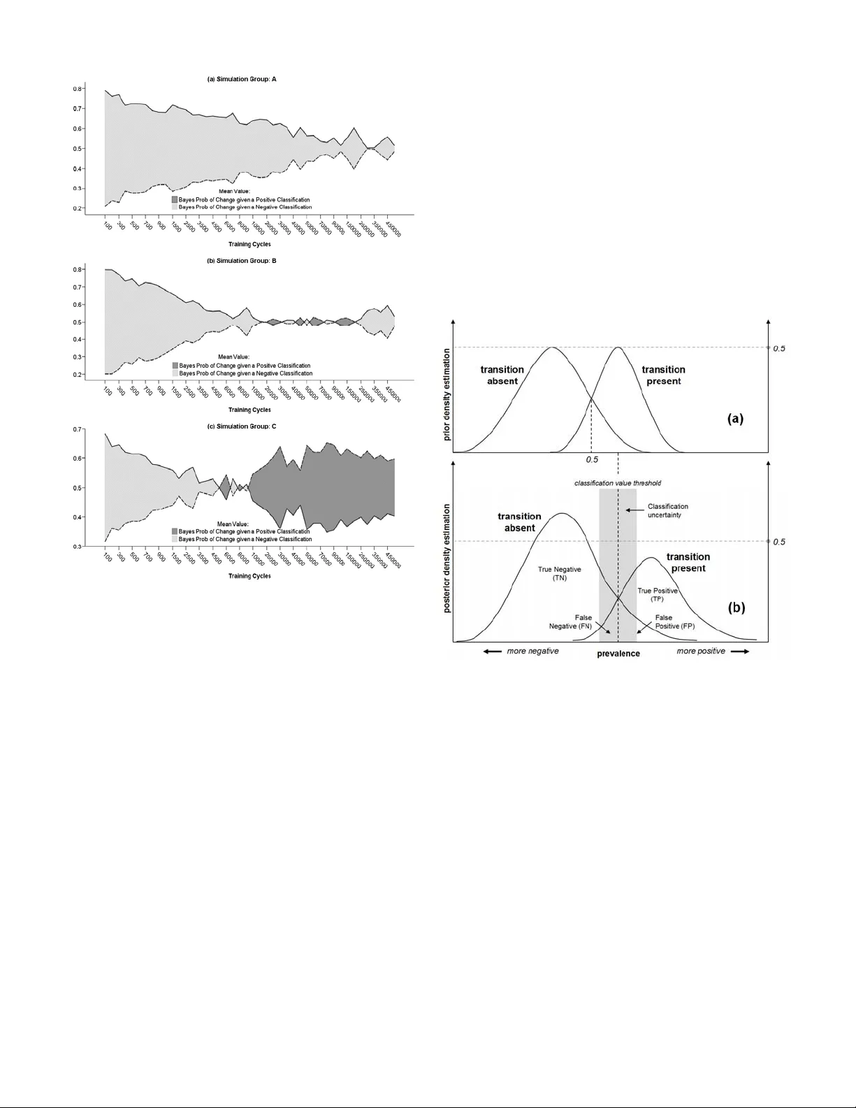
CLN: 8-439 1 Developing Bayesian Information Entropy- based T echniques for Spatially Explicit Model Assessment Kostas Alexandridis and Bryan C. Pijanowski Abstract — The aim of this paper is to explore and develop advanced spatial Bayesian asse ssment methods and techniques for land use modeling. The p aper provides a comprehens ive guide for assessing additional informational entropy value of model predictions at the spatially explicit domain of knowledge, and proposes a few alternative metrics and indicators for extracting higher-order informat ion dynamics from simulation tournaments. A seve n-county study are a in South-Eastern Wisconsin (SEWI) has been used to simulate and assess the accuracy of historical land use changes (1963-1990) using artificial neural netw ork simulations of the Land Transformation Model (LTM). The use of the analysis and the performance of the metrics helps: (a) understand and lear n how we ll the model runs fits to different combinations of presence and abs ence of transitions in a landscape, not si mply how well the model fits our given data; (b) derive (estimate) a theoretical accuracy that we would expect a model to assess under the presence of incomp lete information and measuremen t; (c) understand the spatially explicit role and patterns of uncertainty in simulations and model estimations, by comparing resul ts across simulation runs; (d) compare the significance or estimation contribution of transitional presence and absence (chan ge versus no change) to model performance, and the cont ribution of the spatial drivers and variables to the explanator y value of our model; and (e) compare measurements of information al uncertainty at different scales of spatial resolution. Index Terms — Neural network applications, Uncertaint y, Complex Systems; Bayesian Inform ation. I. T HE NEED FOR SPATIALLY COMPLEX STOCHASTIC MODELING ASSESSMENT he aim of this approach is to explore and develop advanced spatial assessm ent methods and techniques for land use intelligent modeling. Tr aditional statistical accuracy assessment techni ques, although essential for validating observed and historical land use changes, often fail t o capture the stochastic character of the modeling dynami cs. The research presented here provides a comprehensive guide for assessing additional informat ional entropy value of model predictions at the spat ially explicit dom ain of knowledge. It proposes a few alternative m etrics and indicators that encapsulate the ability of the modeler to extract higher-ord er information dynam ics from simula tion experiments. The term information entro py , orig inates from the information-theoretic concept of entropy, conceived by C laude Shannon on his famous two articles of 1948 in Bell Sy stem Technical Journal [1], and expanded later in his book “M athematical Theory of comm unication” [2]. Since the mid-20th cent ury, the field of information theory has experienced an unprecedented development, especiall y following the expansion of computer science in almost every scientific field and d iscipline. The concept of entropy in information systems theory allow us to allocate quantitativ e measurements of uncertainty containe d within a random event (or a variable describing it) or a signal representing a process [3, 4]. Manuscript received June 2008. This work was supported in part by a Purdue Research Foundation (PRF) Fellowship, the US National Science Foundation (Grant WCR:0233648), the E PA STAR Biological Classification Program, the Great Lakes Fisheries Tr ust, and the Purdue University Department of Fore stry and Natural Resources. K. Alexandridis is a Research Scientist (Regi onal Futures Analyst) with the Comm onwealth Scientific and Industrial Research Organization (CSI RO), Division of Sustainable Ecosystems, CSIRO Davies Laboratory, University Drive, Douglas, QLD 4814, Australia (phone: +61 7 4753 8630; fax: +61 7 4753 8650; e-mail: Kostas.Alexandridis@csiro.au). B. C. Pijanowski , is an Associate Professo r with Purdue University, Department of Forestry and Natural Resources, West Lafayette, IN, USA (e - mail: bpijanow@purdue.edu). The literature on assessing spatially exp licit models of land use change has made subst antial steps during the last few years. Many of the metrics and assessment techniques in the past have been treating land use predi ctions as complex signals, and models themselves often are treated as measurem ent instruments, not different from signal- measurement devise assessm ent in physical experiment s [5]. Spatially expl icit methods and assessm ent techniques are used in many remote sensing applicatio ns [6]; wildlife habitat models [7]; predicting presence, abundance and spatial distribution of populat ions in nature [8]; analyzi ng the availability and management of natu ral resources [9, 10]. In a more theoretical level of analysis, spatial ly explicit m ethods of model assessm ent have been used for testing hypotheses in landscape ecological m odels [11, 12]; address statistical issues of uncertainty i n modeling [10] ; or analyze landscape-specific characteristics and spati al distributions [13]. Methodologies and techniques as the ones referenced above often maintain and preserve traditional statistical approaches to modeling assessment. Most lik ely, they test the limitations and assu mptions of statistical techn iques orig inally designed for analyzing data and variabl es that do not exhibit spatially explicit variation. The majority of studies where T CLN: 8-439 2 spatially expli cit methodologies are used t end to involve relatively simple or lin ear statistical analyses [14, 15]. W hile in the recent years assessment of modeling com plexity has been an issue of analysis [16, 17], has y et to include spatia l complexity and assessment of stochasticity as essential elements of evaluation and anal ysis. Spatial complexity by itself is not often enough to fully describe and represent the complex syst em dynamics of coupled human and natural systems. The i ntroduction of spatial complexi ty in advanced dynamic m odeling environments requi res the involvement of stochasticity as an essential element of the modeling approach. It rests between traditio nal spatial assessment and game- theoretic approach es to modeling. The level o f uncertainty and incomplet e information embedded on the com ponents of a coupled human-biophy sical system often necessitates the introduction of stochasti city as a measurable dim ension of complexit y [18, 19]. Stochastic modeling i s widely introduced in modeling com plex natural and ecological phenom ena [20], population dynam ics [21], spatial landscape dy namics [22], intelligence learning and knowle dge-based systems [23], economic and utility modeling [24, 25], decision-making, Bayesian and M arkov modeling [26, 27] and m any other associated fields in science and engineering applicat ions. A natural extension of the relate d techniques and methodologi es is the development and introduct ion of spatially explicit, stochastic methods of accuracy assessm ent for intelligent modeling. In recent years, methods, techniques, and measures of informationa l entropy exceeded the single dimensionality of tradition al statistical techniques (i.e., measuring uncertainty on single random events or variables) and begun analyzing multi-dim ens ional signals. The concept of spatial entropy [28, 29] presents analysis of informational entropy patterns in two-dimensional sp atial systems. Within these lines, the remaining of the p aper introduces so me alternative metrics that aim to assist and enhance the power of our inferential mechanisms in modeling such systems. II. A CASE - STUDY : ANN S IMULATIONS IN S OUTH -E ASTERN W ISCONSIN REGION The study is based on modeling hi storical urban spatial dynamics using Artificial Neur al Network (ANN) sim ulations for a large spatial region of Sout h-Eastern Wisconsin (SEWI) in the Midwestern regio n of U.S. The details of the simulation can be found in a recent paper by Pijanowski et al. [30], where the modeling dy namics and a comprehensive descripti on of the LTM modeling m echanism and experiment al design is deployed. Description of t he LTM model is also provided in Pijanowski et al. [31, 32]. A. Sampling Methodology The project area involves a seven-county region in the South-Eastern Wisconsin (SEWI) region, and includes the city of Milwaukee and its wider suburban area [33]. The land use changes that occurred in the SEWI region during the period 1963-1990 is considerable. Most of the urban growth has taken place in the suburban metropolitan Milwaukee region, and the areas around medium and large cities in the region ( Fig. 1 ). The county of Waukesha, in the west side of the city of Milwaukee has absorbed the majori ty of suburban changes, but import ant urban and suburba n changes have occurred in the remaining countie s both at the North (Washington and Ozaukee counties) and South (Walworth, Racine and Kenosha counties) of the city o f Milwaukee. Fig. 1: Land use changes in the SEWI re gion, 1963-1990. The large size of the area unde r study, and the ability to perform extensive traini ng and learning simulations usi ng the LTM model, m akes computationall y impossible to sim ulate the entire region as a whole. Instead, a comprehensive sampling m ethodology has been implem ented. The regional extent of the SEWI area has been divided into equal-area square boxes of 2.5 square k ilome ters (or 6889 cells of 30 m 2 resolution). The square sampl ing boxes vary on both num ber of cells that experienced urban change duri ng the 1963-1990 period, and the amount of exclusionary la nd zones (urban zones in 1963, paved roads, water bodies, protected areas, etc.). Both parameters affect the m odeling performance and the ability to assess compara tively the accuracy of the modeling predict ions. Thus, random sampling schem e has been implemented for this modeling exercise ensuring comparative assessment of the q uantities and spatial p atterns of land use change in the region. First, t he regional sampling boxes has been ranked and classified using a com bined index of both proportion of urban change and proporti on of exclusionary zone within the sam pling box. The yielded combined ranking index t akes account of both changes within the sampled boxes and represents the ratio between the percentage of urban change and the percentage of variat ion in exclusionary zone areas across the sample d boxes 1 : %( ) %( ) s urban I exclusio nary Δ = Δ (1) where s = number of area sampl ing boxes in the landscape. 1 In LTM model, an exclusionary z one is defined as the m ap area where model pattern training and simulation are not implem ented, i.e., areas with no suitability for transitional change. Exampl es of these zones include m ap areas CLN: 8-439 3 From the continuous sam pling index values derived from the previous step, two threshold values of the sampl ing index have been used to define three classificati on index regions for random sam pling. The sampling boxes have been assigned into three sequential cl assification pool groups (group A, B and C), according to the fo llowing rules (thresholds): A0 1 : B 2 C1 s s s if I Sampling Pool Group if I if I ≥ ⎧ ⎪ ≥ ⎨ ⎪ ≥ ⎩ (2) The sampling pool classi fication in equation (2) follows a nested hierarchical scheme, th at is, the prospective sampling pool of each consequent group is contained in the previous one (i.e., sampling pool for group C is fully contained in group B’s sampling pool, and sampl ing pool for group B is fully contained wi thin group A’s sampling pool). Such classification scheme allow th e testing of the effects of increased exclusionary zone ar ea to the model performance in the simula tions. Sampling pool group A contains all boxes in the sampling regi on. Sampling pool group B cont ains only sampling boxes that have no more than double the percentage of exclusionary area than the pe rcentage of urban change area. Finally, sam pling pool group C contains only the sampling boxes that have no more than equal or more percentage of urban change area than exclusi onary zone area within them. The mem bers (sampling boxes) of each sampling pool group (A, B, and C) have been ranked and assigned to 30th q uintiles according to their ascending proportion of urban change within the sample box. From each 30-tile, one sampling box has been randomly sel ected using a random num ber generator algorithm. The seed of t he random number generator has been renewed before each sampling operation. The final outcome of the random sampl ing procedure, was three sampling groups (varying on the ascending ratio of urban to exclusionary zone area), containing thirty 2.5 square ki lometer sampli ng boxes each (varying on the percent of urban change). The sampled boxes for area groups A, B and C are shown in the following Fig. 2 . Fig. 2: SEWI random sampling groups A, B and C. B. Simulation Modeling Paramet erization The LTM model requires three level s of parameterization: that already undertook transitions before the sim ulations’ initialization; road and transportation system extends; preserved natural areas, etc. (a) the simulati on drivers of land use change; (b) the training and testing neural network pat tern creation; and, (c) the network simulati on parameter definition. Detai ls on the theoretical neural network sim ulation parameterizati on of the LTM model are reported in th e literature by Pijanowsk i et al. [31, 32]. Explicit description of the modeling enterpri se in the SEWI region are also reported in the Pijanowski et al. [30] paper. In short, eight simulat ion distance drivers of land use change has been used to parameterize the LTM simulations (urban land in 1963, historical urban cente rs in 1900, rivers, lakes and water bodies, highways, st ate and local roads, and lake Michigan). The simula tion model uses every other cell (50% of the cells) as neural network training pattern, and the entire region for network m odel testing. Finally, the network is trained for 500,000 traini ng cycles, by resetting and iterating the network node’s weight confi guration every 100 training cycles, and outputting t he network node structure and the mean square error of the network convergence every 100 cycles in a file. Thus for each of the 90 sam pled boxes, the simulat ion output a total of 5,000 network files and MSE values for a grand total of 450,000 simulat ion result files. For simplicity of presentation, in each of the sampled boxes, forty- four of these network output file s are selected for visuali zation of the results. Due to the nature of the neural network learning dynamics, l earning patterns follow a negative exponent ial increase through training iterati ons. Thus, a negative exponential visualizati on scale has been chosen to visualize the results (m ore frequent samples in lower network training cycles, less frequent sam ples in higher training cycles). The simulat ion results for urban change predictions in 1990 are assessed against historical land use changes i n 1990 from existing data provi ded by the Southeastern Wisconsin Regional Planni ng Commission [33] . III. M ETHODOLOGY AND RESULTS OF THE S IMULATION A CCURACY A SSESSMENT The paper by Pijanowski et al. [30], reports three rela tive conventional statistical metric s for the quantitative accuracy assessment of the model performance. Nam ely, the percent correct metric (PCM), the Kappa metric (K), and the area under the receiver operator characteristic curve (AROC) metric. The PC M metric is a sim ple proportional m easure of comparison, whil e the K and AROC metrics ta ke into account the confusion mat rix and the omission and comm ission errors of the simulat ion. In addition to these three conventional metrics 2 , two more alternative metrics are presented here. Namely, the Bayesian predict ive value of a positive and negative classifica tion (PPV and NPV) metrics, and the Bayesian conversion factor (C b ) metric. These alternative metrics measure a stochastic level of in formation entropy in the simulated land use change system. They represent 2 The discussion involving these three me trics is largely om itted from this paper. The reader can consult the rela tive literature, and the Pijanowski et al. CLN: 8-439 4 different aspects or dim ensions of the predictive value of information that is embedded in the simulation model results, and thus, can enhance our understanding of both simulation dynamics, and t he dynamics of the land use change system . A. Basic Definitions The notion of spatial accuracy assessment utilizes three major assumptions. The first assumption has to do with th e underlying process in hand. In any given landscape, two theoretical observers (e.g., a sim ulation model and an observed historical ma p, or a simulation model and another simulat ion model, or an observed historical map and an alternative historical map) are assumed to observe properties of the same underly ing process (the “real” land use change). The second assumption has to do with the observers themselves. They are assume d to face a theoretical level of uncertainty (regardless the degree o f, small or large). A simulation model is facing uncertainty o n its predicted landscape as a part of the problem formulation (and thus a trivial assum ption), but observed historical landscapes are al so subjects to an implicit degr ee of uncertainty (i.e., measurement errors, rem ote sensi ng classification errors, etc.). These degrees of uncertainty are not necessarily equal between the two observers. The third assum ption involves the assessment process itself. It a ssum es that the two observers acquire their observations (cla ssification) independently from each other. In other words, th e historically observed land use map and the sim ulation results are independent (or, the modeling predi ctions are not a function of the real change in the maps). The independence assum ption is easily to assume in the case of assessing a simulated and an observed landscape, but it becom es nontrivial when non-parametric analysis is used to compare two modeled landscapes, in cases where the same m odel with different configuration is used. A parametric approxim ation of spatial accuracy assessment is based on the notion of a confusion m atrix [34, 35] shown in Table 1 . For binary land use cha nges (i.e., presence-absence of transition), the confusion matri x is a 2×2 square matrix with exhaustive, and mutually exclusive elements. Table 1: Theoretical confusion matrix for binary spatial accuracy assessment. Simulated versus historical land use ch ange ( TN: true negative, TP: true positive, FN: false negative, FP: false positive, SN: sim ulated negative, SP: simulated positive, RN: real negative, RP: real positive, GT: grand total). (2007) paper for more inform ation. Only their value and performance for the simulation experim ents in the SEWI region will be report. A nonparametric approxim ation of spatial accuracy assessment employ s the use of the confusion matrix in somewhat more complex forms. It assesses the sensitivity coefficient as the observed fraction of agreement between the two assessed landscapes, or, in o ther words, the probability o f correctly predicting a tran sition when this tran sition actually occurred in the observed historical data. Sym bolically (S=simulated, R=real), (1 | 1 TP Sensitiv ity p S R TP FN ) = == = + (3) Similarly, the specificity coefficient in equation (4) represents the observed fracti on of agreement between two assessed maps, or, in other words, the probab ility of correctly predicting an ab sence of transition, when this transition is actually absent from the historically observed dat a. Symbolically, 1( TN Spec ificity p S R TN FP 0 | 0 ) − == = + = ) (4) A theoretical perfect agreement between the two observers would require that, (1 | 1 ) ( 0 | 0 , 1 pS R pS R or Sensitiv ity Spec ificity = == = = =− (5) The degree of deviation from the rule as defined in equation (5) , represents the degree of deviation from a perfect agreement between the two cla ssifications, or the degree of disagreement bet ween a modeled (simulated) and an observed (historical) landscape transition . The binary character of the classification schemes requi res the two transition classifications to be exhaustiv e and m utually exclusive. The theory of statistical probabilitie s suggests that a random (fully uncertain) classification between the prob abilities denoted by sensitivity and specificity co efficients would be: 1 2 Sensitiv ity Specif icity = = (6) In other words, for each cl assification threshold (e.g., amount of urban change) in our assessment, a given cel l has an equal (prior) chance (50%) to undergo a land use change transition, not u nlike the tossing o f a coin. B. Bayesian Predictive Value of Positi ve and Negative Classification metric (PPV / NPV) 1) Diagnostic Odds Ratio ( DOR) From the definitions o f sensitivity and sp ecificity in the previous session, we can compute the likelihood ratio m etric [36, 37]. In a binary (Bool ean) classification schem e, there are two forms of li kelihood ratios: the likelihood rat io of a positive classification (LR+), and the likelihood rati o of a positive classification (LR-). The likelihood ratios are connected with the levels of sen sitivity and specificity directly [38]: 1 1 s ensitiv ity sensitiv ity LR and LR s pec ificity spec ificity − += −= − (7) The likelihood ratios obtained for a binary cl assification can be used to compute the value of an index for diagnost ic CLN: 8-439 5 inference, namely, the diagnostic odds rat io (DOR) index. The DOR represents simply the ratio of th e positive to the negative likelihoods: (1 ) (1 ) LR sensitivity specific ity DOR LR spec ificity sensitiv ity +⋅ == −− ⋅ − (8) The DOR can be interpreted as an unrestricted measure of the classification accuracy [ 38], but suffers from serious limitations, since both LR+ and LR- are sensitive to the threshold value (cut-off point) of t he classification [39]. Thus, DOR can be used as a measure of the classification accuracy in cases where, (a) the threshold value of the binary classification is somewhat balanced (around 0.5), or; (b) when comparing classificat ion schemes that have the same threshold value (e.g., in the case of simulat ion runs that are unbalanced but face similar threshold values). In the case of the SEWI region simula tion runs, the DOR can be used to com pare classification performance across training cycles (same areas, and same classification t hresholds), but not across area groups or different sim ulation boxes. The results shown in Fig. 3 a, signify the im portance of pattern learning (training) process of improving the classification accu racy in the SEWI region experimental simulations. Fig. 3: (a) Diagnostic Odds Ratio (DOR) index across LTM training cycles in the SEWI region; (b) Bayes proba bility of change given a positive classification (PPV); (c) Bayes proba bility of change given a negative classification (NPV) me tric results by simulation group in the SEWI r egion. 2) Bayesian Predictive Values In place of the simple and pr actically limited DOR index to assess the robust spatial model accuracy, a Bayesian framework of assessm ent can be used. It uses the likelihood ratios (LR+ and LR-), to estimate a posterior probability classification based on the informati on embedded in the dataset. Strictly speaking, th e model accuracy obtained by the confusion matrix (and conseq uently the sensitivity an d specificity values), represents a prior probabilistic assessment of the model’s accuracy. This assessm ent is subject to the threshold value of the classification schem e. Obtaining a classification schem e that is robust enough to allow us to estimate model accuracy for a range of thresholds, requires the computati on of the conditional estimat es [40]. This represents a posterior probabilistic assessment of the model’s accuracy, and can be achieved using Bayes’ Theorem. Computi ng the posterior Bayes pro babilities for a positiv e and negative classification can be achie ved using a general equation form: () ( ) (| ) () ( ) () ( 1 ) px p c PPV p x c px p c px p c + + +− ⋅ == ⋅ +⋅ − (9) and, () ( 1 ) (| 1 ) () ( 1 ) () ( ) px p c NPV p x c px p c px p c − − −+ ⋅− =− = ⋅− + ⋅ (10) where, PPV: the Bayes predictive valu e of a positive classification metric; NPV: the Bayes predictive value of a n egative classification metric; , x x + − : the positive an d negative v alues of the classification, and; : the prevalence threshold for which a value is pos itive if it is larger or equal from (computed using a M L nonparametric estim ation). c The PPV and NPV values can be computed from the sensitivity and specificity values (and thus from the confusion matrix) as follows: (1 ) (1 ) sens prev PPV s ens pr ev s ens prev ⋅ = ⋅+ − ⋅ − (11) and, (1 ) (1 ) (1 ) (1 ) spec prev NPV s pec pre v sens prev −⋅ − = −⋅ − + ⋅ (12) The results for the PPV and NPV metrics obtained for the SEWI region and the three sim ulation area groups are shown in the following Fig. 3 b,c. Simulation area group C has consistently the higher PPV and the lowest NPV throughout the training exercise, a fact that signifies a higher m odel performance level than the ones achieved by simulation area groups A and B. Measuring and treating PPV and NPV as separate m etrics of model performance is a rather trivial operatio n, and it is not a very useful or inform ational tool in assessing spatial model accuracy. However, by combining the PPV and NPV metrics into a single g raph, we can illustrate th e dominance relationships and dynami cs over an expected prevalence threshold value (i.e., prevalence= 0.5, denoting an uninformati ve prior for the Bayesian classifi cation). Fig. 4 shows the dominance relationshi ps between PPV and NPV for increasing LTM training cycles. In sim ulation area group A, the model accuracy is based ma inly on the dominant negative classification (although t his dominance fades over the training process). The accuracy in simulation area group B is based on an unstable equilib rium between positive and negative classification (especiall y between 20,000 and 250,000 training cycles), although the overall accuracy is still supported by a dominant negative classification scheme. The m odel accuracy in simulati on area C depends on a more desired cl assification scheme, since after the first 10,000 cycles model accuracy depends con sistently on a positiv e classification. CLN: 8-439 6 Fig. 4: Dominance relations between Bay es PPV and NPV metrics: (a) area group A; (b) area group B; (c) ar ea group C. The analysis of the latter resu lts is based on an expected, i.e., balanced prevalence thresh old. In reality, the relationship between Bayesian predict ive values and prevalence is non- linear and it is defined by the posteri or Bayesian estimator properties, name ly the posterior density esti mation [36, 41]. To understand the role of the posterior Bay esian estimation, a theoretical problem formulation is provided in Fig. 5 . Part (a) of the figure provides a hypothetical prior densi ty estimati on of a binary classification scheme across a continuous range of classificati on thresholds (prevalence). For a given transitional change (e.g., presence of land use change), the prevalence threshold ranges from zero (purely negative) to one (purely po sitive). The left density curv e represents the absence of a transition (nega tive classification), while the right density curve represent s the presence of a transition (positive classification). As ex plained in the first section, when we lack any additional information about the classification threshold, the best uncert ain choice (maximum entropy classification), is to assume an equal probability between the two classes (present, absent). In most of the cases involving spatial accuracy assessm ent, an uncertain prior is the best choice. Unlike the ROC curve method, where accuracy is assessed using a nonparametric estimation (without the use of a distri bution function), the Bay esian estimation is based in a parametric assessment of the classification accuracy (or, at least a semiparam etric assessment). In such an uncertain classification, we can vary only the spread of the distri bution (i.e., the width of the density distribution) for each of the classes, but not the location of the threshold. As a consequence, the am ount and proportions of the false negative (FN) and false positive (FP) allocations are affected only by the difference on the mean value of each of the transitions to the threshold. The more this difference is positiv e, the more likely it is for the transition to be present, wh ile the more the difference is negative, the more likely it is for the transition to be absent. Fig. 5: Properties of the Bayesian estim ation in binary classification scheme: (a) prior density estim ation; (b) posterior density estimation. Bayesian estimation allows us to estimate the probability densities of the classification s by adjusting the “true” height and “true” width of the density distributions. In Fig. 5b, the changes in the density distributions for the threshold classes shifts the threshold prevalence value disproporti onal to the size and spread of each of th e distributions. The posterior Bayesian density estimates allow us to evaluate the mean and variance of a new, “informative” prevalence threshold (shown with dotted line and shaded areas in Fig. 5 b). In the SEWI region, the relationship between prevalence and the level of th e PPV/NPV is shown in Fig. 6 . The y-axis of the graph represents the prevalence level (classification threshold), wh ile the x-axis represen ts the level of the predictive value (PPV or NPV). The point s that belong to the PPV and NPV are color-coded. The data points correspond to all sample d simulation runs (44 sam pled training cycles for each of the 90 boxes in groups A, B and C, a total of 3,960 simulation run results). CLN: 8-439 7 Fig. 6: Relationship between prevalence (y-axis) and the Bayes predictive values, PPV and NPV (x-axis). The solid lines represent the Epanechnikov kernel density estimation for PPV and NPV. The dotted reference lines identify the difference between expected and predicted prevalence thresholds. We can perform a nonparametric estimation of the probability density functio n in th e data, by using a kern el density estimator. The solid lines in Fig. 6 represent the results of the Epanechnikov stochastic kernel estimati on [42]. The general equation of the kernel densit y function is [43, 44]: 1 1 ˆ () N i K i x X fx K Nh h = − ⎛ = ⎜ ⎝⎠ ∑ ⎞ ⎟ (13) where, ˆ K f : an unknown continuous proba bility density function; h : a smoothing param eter; () K z : a symmetric kernel function, and; N : the total number of independent observations of a random sam ple X N . The equation for the Epanechnikov kernel density functi on is [43]: 2 31 (1 ) 5 5 () 5 45 0 zi f z Kz otherwise ⎧ −− ≤ ⎪ = ⎨ ⎪ ⎩ ≤ (14) The choice of the Epanechnikov kernel densi ty estimator i s based on the high efficiency on minimi zing the asymptotic mean integrated square errors , AMISE [45, 46], and i t is often used in Neural Network com putational learning [47]. In the SEWI region data, the underlying question that the analysis attempts to address is for which prevalence threshold value the “true” predictive value (and accuracy) of the modeled transitional classificati on becomes equal to the “true” absence of such transaction? Graphically, the solu tion can be found by varying the height of the y-axis reference line (horizontal dotte d lines in Fig. 6 ) over a fixed level of predictive value, where (vertical dotted line). The y-axis coordinat e for which the two kernel densi ty estimated lines meet represents the prevalence threshold that maxim izes the posterior probability of our model accuracy predictions. 0.5 PPV NPV == Mathematically, the optimal prevalence threshold of the posterior pro bability distribution exists where: ˆˆ () () KK f xf x + − = (15) The difference between the prior and posterior estimation is shown in the vertical distance between the y-axis reference lines at the 0.5 prevalence threshold and the one at the meeting poi nt of the two kernel density functions (~0.172 in the entire SEWI regions’ simulat ion data). The posterior estimation allows us to th reshold at a lower classification level, and thus enhancing th e accuracy of our predictions. 3) Bayesian Convergence Factor metric (C b ) It is possible to derive an a lternative accuracy metric that combines the two Bayesian pr edictive v alues, PPV and NPV in a single, unified coefficient. The use of such a coefficient to measure classification and model accu racy is that allows us to estimat e not only a unique prevalence threshold, but also an optimal prevalence region for wh ich our estimated accuracy is high for both p ositive and neg ative classifications. The analysis provided in the previ ous paragraph in the case of PPV and NPV metrics depends m ainly on the choice of the kernel density estim ation function and the continuous interval bandwidth used [43, 4 8], or any other pr obability density function used for estimat ion. A unified Bayesian coefficient that measures the level of convergence between positive and negative predictive values perm its us to derive a m ore robust prevalence region that tends to sm ooth the effect of density estimat ion selection. In other words, it provides us with a more global m easure of model and classification assessm ent. We can call this coefficient Bayes convergence factor, C b . A simple form of the factor can be defined as: ( ) 1 1( ) b PPV NPV if PPV NPV C NPV PPV if PP V NPV −− ≥ ⎧ = ⎨ −− < ⎩ (16) A higher level of the Bayes convergence factor thus denotes higher probability of convergence between a positive and a negative predictive value or pr obabilities of change. Because of the pro bability prop erties of such a coefficient, an d the fact that always 1 PPV NPV + ≤ 1 . 0 (the probability of change cannot exceed 1.0), the range of the C b coefficient will be: 0 b C ≤ ≤ . This simple form of the Bayes convergence factor is shown in the theoretical curve C b (A) of Fig. 7 a. We can see that the allocation o f the positive an d negative classification proba bilities in the C b function represents a form of a triangular densit y function with mini mum value of zero, maxim um value of 1.0, and mean value of 0.5. A triangular density function provi des a minimal amount of inform ation about the relationshi p, configuration and pattern between the positive and n egative predictive v alues in a model. As shown in Fig. 7 a, these predictive values by th emselves may be better represented by non-linear relat ionships (e.g., kernel density CLN: 8-439 8 estimat ors). Thus, a better convergence factor can be found that reflects a degree of nonlinearity in the m odeling classification assessment. Fig. 7: (a) Theoretical distribution density functions for the Bayes convergence metric (Cb): (i) triangular; ( ii) adjusted norm al; (iii) asymm etric normal. (b) Var iations of the asymmetry parameter, α , in the expected norm al form of the Baye s convergence factor. An alternative form of the Bayes convergence factor can be symbolically calculated using a Normal density distribut ion function , adjusted to a continuous scale between 0 and 1.0. The equation of the Normal density function is, 2 2 () 2 1 ˆ (, , ) 2 x N fx e μ σ μσ πσ ⎛⎞ − − ⎜⎟ ⎜ ⎝ =⋅ ⎟ ⎠ (17) For a Normal distribut ion with and 0 x = 0.5 σ = , we can model the behavior of t he mean value, by setting, PPV NPV μ =− (18) and thus, () () () 2 2 2 0 2(0 . 5) 2 1 ˆ (0 , , 0. 5) 2( 0 . 5 ) 0.797885 PPV NPV N PPV NPV fP P V N P V e e π ⎛⎞ −− ⎜⎟ − ⎜⎟ ⎜⎟ ⎝ −− −= ⋅ =⋅ ⎠ (19) We can adjust for the coeffi cient scale (0 to 1.0), by multiplying the previou s equation by a n ormalization factor, 1 0.797885 2 πσ = (20) The adjusted Normal form of the Bayes convergence factor, can expressed as: ( 2 2 PP V NPV b Ce −− = ) (21) The adjusted normal densi ty distribution function of the C b coefficient can be seen in the curve C b (B) of Fig. 7 a, and in our data can be estim ated by a Normal or Epanechnikov kernel density functi on. The previous two forms of the C b metric assume implicitly that the combined effect of the po sitive and negativ e classification pro cess in our model is symmetric toward achieving a better model (and cla ssification) accuracy. It is appropriate for m odeling changes where the presence of a transition implies the absence of a n egative transition. In many spatial m odeling processes simulating binary change that impli cit assumption cannot be made easi ly. For example, a model (such as LTM) that si mulates land use change is parameteri zed and learns to recognize patterns on drivers of change related to a positiv e land use transition effect o nly. Model training and te sting based on drivers of transi tional presence, do not necessarily convey inform ation on the probability o f absence of such a transition, as it is likely that other or additional drivers of t he absence of the transition may be in effect over an ensemble of landscapes. Consequently , we can derive a better form of t he Bayes conversion function by assuming a biased or asym metric join distri bution among the predictive v alue of po sitive and negativ e classification. Such an asymmetry would favor more positive th an negative classifications, assum ing that the model learns m ore about the transitional patterns from a combination o f a high positiv e and low negative p redictive value, rather th an from a high negative and low pos itive predictive v alue (since the sum of the predictive valu es equals 1). The later is especially important in estimating empi rical distributions derived from unbiased real-world data, such as in the SEWI case study. The amount of area that undertakes urban land use transition in the data is considerably less than the am ount of area that observes an absence of such trans ition, and impl ementing an asymm etric Bayesian prior di stribution would assign m ore weight in the positiv e (presence of transitio n) than in the negative (absence of transition) land areas. We can formulate such a conversion function from modifyi ng the mean central tendency of the previous form , C b (B) . In other words, by simula ting a different mean for the adjusted Normal distribut ion function. We can call this form, adjusted asymmetric Normal density distribution , and for the same num erical parameters, , and 0 x = 0.5 σ = , we can simulate t he behavior of the mean value, ( ) PPV NPV μα ′ =− − (22) where, α is the degree of asymmet ry of our distribution ( 01 . 0 α ≤ ≤ ). In other words, the parameter α denotes the degree of bias in terms of a theoretical least-cost function , or the relative info rmational balance in ou r model from a positive to negative pr edictive value. The new asymmetric normal distribution will be, () () () () 2 2 2 0 2(0 . 5) 2 0, ( ), 0.5 1 ˆ () 2( 0 . 5 ) 0.797885 PPV NPV N PPV NPV PPV NPV fe e α α α π ⎛⎞ −− − ⎜⎟ − ⎜⎟ ⎜⎟ ⎝⎠ −− − −− =⋅ =⋅ (23) and, after adjusting for scale normali zation, the final Bayes convergence factor, will be, ( 2 2 PP V NPV b Ce α −− − = ) (24) For varying levels of t he parameter α , the shape of the latter convergence factor is shown in Fig. 7 b. For 0 a = , the equation yields t he symmetric normal form of the convergence factor (i.e., shape C b (B) in Fig. 7 a), while, for 1.0 a = , the equation yields a full asymmetric normal form of the convergence factor (i.e., shape C b (C) in Fig. 7 a). In an experimental dataset, any form of asym metric norm al distributi on form of C b (i.e., for any parame ter α ) can be estimat ed by a Normal of Epanechnikov kernel distributi on function. CLN: 8-439 9 The results of the empi rical data obtained for the SEWI region simulati on runs for the varying degree of asymmet ry in estimati ng the Bayes Convergence Factor, C b , are shown in Fig. 8 a. We can see that a somewhat moderate level of asy mmet ry ( 0.25 α = ) performs consistently better throughout the entire model learni ng process (training cycles), despite the fact that at the 500,000 cycl es training cycle level, the Bayes Convergence Factor with 0.5 α = performs slightly better. Thus, there is evid ence in the SEWI simulation runs that a level of asymmetry in the composition of pos itive and negative predictive value of our model exists, and thus should be incorporated into our spatial accuracy assessment. Fig. 8: (a) Estim ated mean Bayes convergence factor for varying levels of the asymm etry coefficient in the SEWI region; (b) Estimated probabilities of transition from the em pirical values of the Bayes convergence factor ( α =0.25). Data points represent the estimated PPV and NPV values in the SEWI region (for all simulation boxes’ sam pled training cycles). Beyond any visual inspection and inference of our results, it is possible to derive q uantitative estimates of the dominance of a level of asymm etry present in our sim ulation runs. As can be seen in Fig. 8 b we can estimate the expected probab ilities of transitions, subject to the observed empi rical values of transitions pr esent in our simulation d ata. When all the simulation runs results for the entire SEWI region are examined with respect to their respective observ ed predictive values, we can estimate such an empirical prob ability distribution, as a function of an estimated “true” mean (location param eter) and standa rd deviation (scale param eter) of each of the forms of Bayes Convergence Factor, , using a maxim um likelihood esti mation ( ML ) method. The result s of such estimation for the varying degree of asymm etry in the Bayes convergence factor in the SEWI data are shown in ( ˆˆ , bb NC C f μσ ) Table 2 . Two groups of parameter estim ates are included in the analysis: (a ) parameter estim ates across all SEWI simulat ion training cycles, indicating a robust model performance; (b) param eter estimates only after 500,000 training cycles in t he SEWI simulation runs, indicating a model perform ance with emphasis on maxi mizing the information flows in modeling transitional effects in o ur landscape. Table 2: Estimated values for the location ( μ ) and scale ( σ ) param eters of the empirical asym metric Bayes Convergence Factor in the SEW I area. Fig. 9 plots the empirical ly obtained estimated parameters for location (x-axis) against s cale (y-axis). Such a plot can help us select the best asym ptotic form of the Baye s convergence factor using a dominance criteri on, such as the mean-variance-robustness criterion. A desired prob ability distribution would have an estimated m ean value closer to the 0.5 prob ability threshold (prev alence). Thus, estimated location parame ters closer to 0.5 are dominant. On the other hand, we want ou r predicted pro bability distributions to minim ize the level of uncertainty in our predictions. Thus, estimated scale parameters with smaller values are dom inant. Finally, a desired prob ability distribution wo uld have relative consistent estimated values of the location and scale parameters i n both robust and informational assessm ents. We can see from Fig. 9 that the only asymmetric form of the Bayes convergence factor that meets all three dominance criteria is the one with 0.25 α = . CLN: 8-439 10 Fig. 9: Estimated location ( μ ) and scale ( σ ) parameters of selected asymm etric normal form s of the Bayes convergence factor from em pirical data in the SEWI region: (a) robust estim ates (across all training cycles); (b) maximum information estim ates (after 500,000 cycles). We can further enh ance the quantitativ e assessment of the dominant asymmetric form of the C b metri c, by computing explicitly the do minance criteria. The three dominance criteria can be combined as, () () () () ˆˆ ˆ ˆ (, ) ( , ) , : ˆˆ 0.5 0 .5 ˆˆ ˆˆ 0.5 0.5 ˆˆ Ni i N j j ii ii mk jj jj mk f f if and only if m k μσ μ σ μμ σσ μμ σσ ∀≠ −− ⎛⎞ ⎛⎞ −≥ ⎜⎟ ⎜⎟ ⎝⎠ ⎝⎠ ⎛⎞ ⎛⎞ −− ⎜⎟ ⎜⎟ − ⎜⎟ ⎜⎟ ⎝⎠ ⎝⎠ ; (25) where, the symbol “ ; ” denotes dominant rela tionships, and, , ij : unique combinat ions of location and scale (i.e., asymme tric forms of the C b metric). , mk : unique groups for testing robustness (i.e., training cycle groupings). ˆ 0.5 0.5 i ˆ j μμ −− ; : mean (location) criterion ˆˆ ij σ σ ; : variance (scale) criterion () ( mk mk i ) j δ δδ δ −− ; : robustness criterion, and δ : any value or classification rule. The results of the dominance cr iteria in the SEWI results visualized in Fig. 9 are summa rized in Table 3 . The values of the table cells represent the va lues of the differences in equation (25) . The shaded cells signify the dominant asymm etric form of the Bayes convergence factor to be chosen. Table 3: Table 3. Dom inance values for assessing the selection of the Cb asymm etric normal form in the SEWI region. Selecting the appropriate asymmetric form of the Bayes convergence factor allow us to infer additional information about the overall performance of our m odel. We can measure the deviation from a sym metric normal distribution (expected prior probabilities) that the estim ated asym metric form of the Bayesian convergence factor (observed posterior probabilities) yields. The P-P pl ots of this assessment are shown in Fig. 10 . The thick curve represents the estim ated cumulative probability distri bution of the asym metric C b predictive values observed in the SEWI region, and estimated from the sim ulation data. The estimated parameters (location, scale) are shown in the right side of each graph. The diagonal line represents the expect ed cumulative probability distribution of a symm etric dist ribution of predictive values (i.e., the expected predictive va lues at a prevalence threshold of 0.5). The parts of the pr edicted cumulative distribution curve that are above the expect ed one (diagonal) signify an increase in model accuracy th at can be obtained from an asymmetric classification, while the parts of the predictive cumulative distribution curve below the expected diagonal line, signify a decrease in m odel accuracy. The point where the two lines meet (shown as the point of intersection of the reference lines), provide us with an estimated em pirical prevalence level (threshold valu e for classification) that maxim izes the modeling accuracy in our data. The net gain (or loss) in predictive value of our m odel due to the uncertainty in classification is the difference in the area that rests between the expected diagonal line, and the estimated observed curve. CLN: 8-439 11 Fig. 10: Normal P-P plots for assessing Bay esian convergence simulation performance of the SEWI re gion: (a) across all simulation groups; (b) simulation group A; (c) simulation group B; (d) sim ulation group C. From an initial observation of the models’ accuracy within all simulation runs in the SEWI region, shown in sub-graph (a) of Fig. 10 , the estimated prevalence threshold (=0.4) does not seem to deviate importantly from the expected one (0.5). Shifting the prevalence thres hold would provide a 5.7% increase in the predictive valu e (informational gain) of the model. But, if we repeat our analysis for the SEWI regions’ simulation groups (A, B and C), thus accounting for structural differences in the proportion of urban cells and exclusionary areas, we can see that spatial configuration affects considerably our actual model perform ance. For simulation group A, shown in sub-graph (b), the model perform ance is heavily dependent on the negative predictive values (estimated prevalence of 0.53 > 0.5), and produces poor overall model predictive values (Cb=0.436, or a 6.4% decrease in mean predictive value of the model). As the proportion of urban to exclusionary increases in th e spatial composition of our simulation ma ps, the predictive value of the model increases substantially, and the estimated prevalence level decreases. Especially for group C, shown in sub-graph (d), a gain of 19.2% in model perform ance can be obtained from a shift in model prevalence (from 0.5 to 0.23). IV. D ISCUSSION AND C ONCLUSIONS The analysis described above reveals the magnitude and multi-dimensionality of the spatial complexity involved in modeling land use change transitions in mixed and asymm etric landscapes in terms of am ount and distribution of change. Performing spatial accuracy assessm ent requires the development and utilization of additional, advanced m ethods of assessment, related both to the m odels’ predictive value in terms of quantity of change, but also to the performance of classifying the presence or absen ce of such a transition. It has been shown above that classi fication accuracy is closely related to the achieved modeli ng perform ance, and additional Bayesian metrics have been pr oposed, described and analyzed using the SEWI region case st udy. These advanced m ethods take into advantage the stocha stic character of intelligent simulation models such as the LTM model, and can be used for performing m odel assessment in agent-based models of land use change, or other spatia lly explicit artif icial intelligent modeling. The m etrics described in this paper address different aspects of the spatial modeling performance such as assessing the predictive value of the m odel simulations ( PPV, NPV, DOR) , and estimating em pirical convergence curves for enhancing classification accuracy ( C b ). The proposed metrics and their assessment m ethodology allows the researcher and analyst to acquire a more holistic assessment of a models’ spatial accuracy over space and time, especially in the presence of uncertainty a bout the transitional model thresholds. The case study of the SEWI region used to illustrate the usage of the metrics, allow us to make assess the LTM model accuracy for simulating urban changes in the region. All metrics seem to confirm a general emergent m odel accuracy that appears to converge towards a 70% upper level. We can also see how the amount of ur ban change and exclusionary zones present in our landscapes dramatically affects the performance of the m odel. The latter result raises the significance of adjusting th e classification prevalence threshold at spatially homogene ous scales in our simulation groups (e.g., implem enting diffe rent thresholds for groups with different classe s of urban change). The results obtained also allow us to infer that in landscapes where the rate and amount of land use change vary importantly, symm etric spatial transition classification schemes are difficult to obtain. Instead we can enhance model predictions by assuming asym metric spatial configurations, and by estimating the degree of asymm etry via a spatial stochastic dominance methodology. The practical significance of the proposed additional spatia l model assessment metrics is that they can provide an “i nformational sum mary” of the simulated region or landscape ensembles. The use of the analysis and the performance of the metrics can help us in a multitude of ways. First, to understand and learn how well the model fits to different com binations of presence and absence of transitions in our landscapes, not simply how well the model fits our given data. Sec ond, given that most spatial databases suffer from incomplete inform ation and pre- simulation measurem ent errors, we can also derive (estimate) a theoretical accuracy that we would expect our model to assess, under the presence of su ch incomplete information data, and thus partially separate model from measurement errors in spatial simulations. Third, to understand the role and pattern of uncertainty in our simulations and model estimations. We can compare results across simulation runs (and thus quantitative patterns of change) that tend to provide less or more uncertain model performance, and understand the role of spatially-explicit pattern s and cell configurations to model training and sim ulation. Fourth, to compare the CLN: 8-439 12 significance or estimation contri bution of transitional presence and absence (change versus no change) to our model performance, and the contribution of the spatial drivers and variables to the explanatory value of our model. Estimating model perform ance using different combinations of drivers (e.g., instead of groups A, B, C in the SEWI region, use of the same sam pled boxes with different drivers, or using training sets with sequentially dropping a driver at a time), could allow us to estimate the differences in informational uncertainty for each driver combination or fo r single drivers within our simulations. Fifth, to compare m easurements of informational uncertainty at different scales of spatial resolution. Pijanowski et al. (2003; 2005) showed the si gnificance of using a scalable window for sensitivity analysis. Assessing model uncertainty of predictions for each of spatia l resolutions can also enhance our knowledge about modeling at different spatial scales and selecting scales that produce lower uncertainty estimates. Finally, the methodology and m etrics developed in this paper allows for the development of a dynamic and adaptive modeling methodology . Beyond the aggregate level for which the assessment was perform ed for the purposes of this paper, it is both methodologically and com putationally feasible to assess and adjust model accuracy at a sim ulation-to-simulation basis, in order to obtain dy nami cally enhanced simulation results. Especially in the case of agent-based modeling such a model assessm ent methodology can be inversed and iterated to obtain spatially robust and diverse future landscape configurations that optimize both the amount and degree of information contained in the si m ulation, and the emergence of stochastically dominant agent strategies. A CKNOWLEDGMENT Acknowledgments here. R EFERENCES [1] C. E. Shannon, “A Mathematical Theory of Communication,” Bell System Technical Journal, vol. 27, no. July and October, pp. 379- 423 and 623-656, 1948. [2] C. E. Shannon, and W. Weaver, Mathematical Theory of Communication , Chicago, IL: University of Illinois Pr ess, 1963. [3] A. Jessop, Informed assessments : an introduction to information, entropy, and statistics , New York: Ellis Horwood, 1995. [4] I. Vajda, Theory of statistical inference and information , Dordrecht ; Boston: Kluwer Academic Publishers, 1989. [5] P. Stoica, Y. Selen, and J. Li, “Multi-model approach to m odel selection,” Digital Signal Processing, vol. 14, no. 5, pp. 399- 412, 2004. [6] T. Nelson, B. Boots, and M. A. Wulder, “ Techniques for accuracy assessment of tree locations extracted from rem otely sensed imagery,” Journal of Environmental Management, vol. 74, no. 3, pp. 265-271, 2005. [7] G. J. Roloff, J. B. Haufler, J. M. Scott et al. , "Modeling Habitat- based Viability from Orga nism to Population," Predicting Species Occurences: Issues of Accuracy and Scale , pp. 673-686, Washington DC: Island Press, 2002. [8] F. C. James, C. E. McGulloch, J. M. Scott et al. , "Predicting Species Presence and Abundance," Predicting Species Occurences: Issues of Accuracy and Scale , pp. 461-466, Washington DC: Island Press, 2002. [9] C. Gonzalez-Rebeles, B. C. Thom pson, F. C. Bryant et al. , "Influence of Selected Environm ental Variables on GIS-Habitat Models Used for Gap Analysis," Predicting Species Occurences: Issues of Accuracy and Scale , pp. 639- 652, Washington DC: Island Press, 2002. [10] K. Lowell, and A. Jaton, Spatial accuracy assessment : land information uncertainty in natural resources , Chelsea, Mich.: Ann Arbor Press, 1999. [11] M. Cablk, D. White, A. R. Kiester et al. , "Assessment of Spatial Autocorrelation in Em pirical Models in Ecology," Predicting Species Occurences: Issues of Accuracy and Scale , pp. 429-440, Washington DC: Island Press, 2002. [12] J. Wu, and R. Hobbs, “Key issues and research priorities in landscape ecology: An idio syncratic synthesis,” Landscape Ecology, vol. 17, no. 4, pp. 355-365, 2002. [13] D. W . McKenney, L. A. Venier, A. Heerdegen et al. , "A Monte Carlo Experim ent for Species Mapping Problem s," Predicting Species Occurences: Issues of Accuracy and Scale , pp. 377-382, Washington DC: Island Press, 2002. [14] A. E. Gelfand, A. M. Schmidt, S. Wu et al. , “Modelling species diversity through species leve l hierarchical modelling,” Journal of the Royal Statistical Society: Series C (Applied Statistics), vol. 54, no. 1, pp. 1-20, 2005. [15] G. R. Pontius, Jr ., and J. Spencer, “Uncertainty in Extrapolations of Predictive Land-Change Models,” Environment & Planning B : planning and design, vol. 32, no. 2, pp. 211-230, 2005. [16] B. J. L. Berry, L. D. Kiel , and E. Elliot, “Adaptive agents, intelligence, and emergent hum an organization: Capturing complexity through agent- based modeling,” Proceedings of the National Academy of Sciences, vol. 99, no. Supplement 3, pp. 7178-7188, 2002. [17] M. North, C. Macal, and P. Campbell, “Oh behave! Agent-based behavioral representations in problem solving environments,” Future Generation Computer Systems, vol. In Press, Corrected Proof, 2005. [18] K. T. Alexandridis, and B. C. Pijanowski, “Assessing Multiagent Parcelization Performance in the MABEL Sim ulation Model Using Monte Carlo Replication Experim ents,” Environment and Planning B: Planning and Design, vol. 34, no. 2, pp. 223-244, 2007. [19] D. G. Brown, S. E. Page, R. Riolo et al. , “Path Dependence and the Validation of Agent-based Spatial Models of Land Use, ” International Journal of Ge ographical Information Science, vol. 19, no. 2, pp. 153-174, 2005. [20] M. J. Fortin, B. Boots, F. Csillag et al. , “On the Role of Spatial Stochastic Models in Understanding Landscape Indices in Ecology,” Oikos, vol. 102, no. 1, pp. 203-212, 2003. [21] L. Demetr ius, V. Matthias Gundlach, and G. Ochs, “Com plexity and demographic stability in population m odels,” Theoretical Population Biology, vol. 65, no. 3, pp. 211-225, 2004. [22] J. C. Luijten, “A system a tic method for generating land use patterns using stochastic rules and basic landscape character istics: results for a Colombian hillside watershed,” Agriculture, Ecosystems & Environment, vol. 95, no. 2-3, pp. 427-441, 2003. [23] X. Boyen, and D. Koller, "Approxim ate Learning of Dynamic Models." pp. 396-402. [24] J. Dubra, and E. A. Ok, “A Model of Procedural Decision Making in the Presence of Risk,” International Economic Review, vol. 43, no. 4, pp. 1053-1080, 2002. [25] A. Lazrak, and M. C. Quen ez, “A Generalized Stochastic Differential Utility,” Mathematics of Operations Research, vol. 28, no. 1, pp. 154-180, 2003. [26] E. Fokoue, and D. M. Titter ington, “Mixtures of Factor Analysers, Bayesian Estimation and I nference by Stochastic Simulation,” Machine Learning, vol. 50 no. 1-2, pp. 73- 94, 2003. [27] J. P. C. Kleijnen, An Overview of the Design and Analysis of Simulation Experiments for Sensitivity Analysis, Discussion Paper 2004-16, Tilburg University, Center for E conomic Research 2004. [28] A. I. Aptekarev, J. S. Dehesa, and R. J. Yanez, “Spatial Entropy of Central Potentials and Strong Asym ptotics of Orthogonal Polynomials,” Journal of Mathematical Physics, vol. 35, no. 9, pp. 4423-4428, 1994. [29] A. D. Brink, “Minimum Spatial Entropy Threshold Selection,” Vision, Image and Signal Processing, IEE Proceedings, vol. 142, no. 3, pp. 128-132, 1995. CLN: 8-439 13 [30] B. C. Pijanowski, K. T. Alexandridis, and D. Müller, “Modelling Urbanization Patterns in Two Diverse Regions of the World,” Journal of Land Use Science, vol. 1, no. 2-4, pp. 83 - 108, 2006. [31] B. C. Pijanowski, S. Pithadia, B. A. Shellito et al. , “Calibrating a Neural Network-Based Urba n Change Model for Two Metropolitan Areas of the Upper Mi dwest of the United States,” International Journal of Geogr aphical Information Sciences, vol. 19, no. 2, pp. 197-215, 2005. [32] B. C. Pijanowski, B. Shellito, S. Pithadia et al. , “Forecasting and assessing the impact of urban sprawl in coastal watersheds along eastern Lake Michigan,” Lakes and Reservoirs: Research and Management, vol. 7, no. 3, pp. 271- 285, 2002. [33] SEWRPC, Aerial Photography and Orthophotography Inventory (1963-2000) , SouthEastern W isconsin Regional Planning Comm ission (SEWRPC). http://www.sewrpc.org/ , Waukesha, WI, 2000. [34] G. M. Foody, “Status of land cover classification accuracy assessment,” Remote Sensing of Environment, vol. 80, no. 1, pp. 185-201, 2002. [35] S. Sousa, S. Caeiro, and M. Painho, "Assessm ent of Map Similarity of Categorical Maps Using Kappa Statistics: The Case of Sado Estuary." [36] H. Brenner, and O. Gefeller, “Variation of sensitivity, specificity, likelihood ratios and predictive values with disease prevalence, ” Statistics in Medicine, vol. 16, no. 9, pp. 981- 991, 1997. [37] Y. T. Suh, “Signal Detection in Noises of Unknown Powers Using Two-Input Receivers,” 1983. [38] A. S. Glas, J. G. Lijmer, M. H. Prins et al. , “The diagnostic odds ratio: a single indicator of test perform ance,” Journal of Clinical Epidemiology, vol. 56, no. 11, pp. 1129- 1135, 2003. [39] M. S. Pepe, H. Janes, G. Longton et al. , “Lim itations of the Odds Ratio in Gauging the Performance of a Diagnostic, Prognostic, or Screening Marker,” Am. J. Epidemiol., vol. 159, no. 9, pp. 882- 890, May 1, 2004, 2004. [40] J. Schafer, and K. Strimm er, “An empir ical Bayes approach to inferring large-scale gene association networks,” B ioinformatics, vol. 21, no. 6, pp. 754-764, March 15, 2005, 2005. [41] J. E. Smith, R. L. Winkler, and D. G. Fryback, “The First Positive: Computing Positive Predictive Value at the Extrem es,” Annals of Internal Medicine, vol. 132, no. 10, pp. 804-809, May 16, 2000, 2000. [42] J. D. Hart, and T. E. Wehrly, “Kernel Regression Estim ation Using Repeated Measurements Data,” Journal of the American Statistical Association, vol. 81, no. 396, pp. 1080-1088, 1986. [43] B. W. Silverman, Density Estimation for Statistics and Data Analysis : CRC Press, 1986. [44] J. S. Sim onoff, Smoothing methods in statistics , New York: Springer, 1996. [45] R. A. Tapia, and J. R. Thompson, Nonparametric probability density estimation , Baltimore: Johns Hopkins University Press, 1978. [46] M. P. Wand, and M. C. Jones, Kernel Smoothing : Chapman & Hall, 1995. [47] P. Sm yth, "Probability De nsity Estimation and Local basis Function Neural Networks," Computational learning theory and natural learning systems , S. J. Hanson, T. Petsche, R. L. Rivest et al. , eds., pp. 233-248, Cam bridge, Mass.: MIT Press, 1994. [48] B. E. Hansen, “Sample Sp litting and Threshold Estimation,” Econometrica, vol. 68, no. 3, pp. 575-603, 2000.