Timescale effect estimation in time-series studies of air pollution and health: A Singular Spectrum Analysis approach

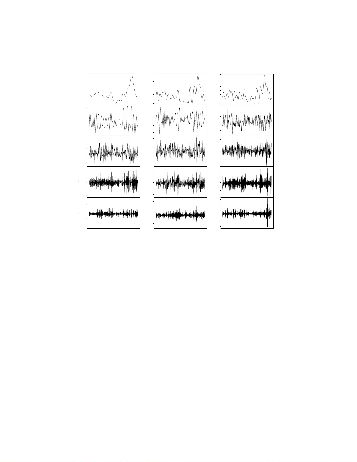
Electronic Journal of Stati stics V ol. 2 (2008) 432–453 ISSN: 1935-7524 DOI: 10.1214/ 07-EJS12 3 Timescale effect estimation in time-serie s studies of air p ollutio n and health: A Sin g ular Sp ectrum An alysis approac h Massimo Bilancia and Girolamo Stea Dip artiment o di Scienze Statistiche “ Carlo Ce c chi” Universit` a de gli Studi di Bari e-mail: mabil@ds s.uniba. it ; stea@dss. uniba.it Abstract: A we alth of epidemiological data suggests an association be- t w een mortality/ morbidity from p ulmonary and cardiov ascular adv erse ev en ts and air pollution, but uncertain t y remains as to the exten t implied by those associations although the abundance of the da ta. I n t his paper we descri be an SSA (Singular Spectrum Analysis) based approac h in order to decom- pose the time-series of pa rticulate matter concen tration in to a set of expo- sure v ariables, eac h one representing a differen t timescale. W e impl emen t our methodology to i n v estigate both acute and long-term effects of PM 10 exposure on morbidity from respiratory causes within the urban area of Bari, Italy . AMS 2000 sub ject classi fications: Primary 62P1 2; secondary 62J99. Keywords and phrases: Airb orne particulate mat ter, PM 10 , Singular Spectrum Analysis - SSA, Gene ralized additive models - GAM. Receiv ed Septem ber 2007. Con ten ts 1 Int ro duction . . . . . . . . . . . . . . . . . . . . . . . . . . . . . . . . . 433 2 Data descr iption and pre-pro c e s sing . . . . . . . . . . . . . . . . . . . 435 3 Singular Sp ectrum Ana lysis . . . . . . . . . . . . . . . . . . . . . . . . 438 4 Eigentriple grouping . . . . . . . . . . . . . . . . . . . . . . . . . . . . 439 4.1 Reconstruction of comp onents . . . . . . . . . . . . . . . . . . . . 439 4.2 Timescale estimation . . . . . . . . . . . . . . . . . . . . . . . . . 443 4.3 Results and so me compariso ns . . . . . . . . . . . . . . . . . . . 446 5 Discussion and conclusions . . . . . . . . . . . . . . . . . . . . . . . . 450 Ac knowledgemen ts a nd additional informatio n . . . . . . . . . . . . . . . 451 References . . . . . . . . . . . . . . . . . . . . . . . . . . . . . . . . . . . . 451 ∗ This wo rk is partially suppor ted by a gran t of the Univ ersit y of Bari - Italy . † Con tacts: Massimo Bilancia, Department of Statistical Sciences “Carl o Cecc hi”, Uni- v ersity of Bari - Via C. Rosalba n.53, 70124, Bar i (Italy). T el: +39(0)805049 341, F ax +39(0)805 049147, E m ail: mabil@dss.uniba.it 432 M. Bilancia, G. Ste a/Timesc ale effe ct estimation 433 1. In troductio n A w ealth of epidemiological studies based on time-ser ies a nalysis ha s shown ev- idence for asso c iation betw een morbidity/mortalit y caused by respirato ry and cardiov ascular adverse even ts and the exp osur e to a irb orne particles [ 3 ]. Sus- pended total par ticulate matter is a c omplex mixture of orga nic and inor ganic substances in either liquid or solid phase. They can v a ry in size, comp osition and or igin and ca n b e characterized both physically and chemically . Particles with an aero dynamic diameter of less than 10 microns ar e referred to as PM 10 : they may b e inhale d r eaching the upp e r airways and the lungs, w ith risk for adverse effects on health. Assuming counts data y t of da ily a dverse health even t b eing distributed as conditionally indep endent Poisson giv en the rate ϕ t , a standa rd ecologica l P ois- son regr ession mo del (which has b een us ed, with minor v ariations, in most of large scale epidemio lo gical studies [ 1 1 ]) is log ( ϕ t ) = β 0 + β 1 PM 10 ,t + [DOW t ] + S ( t, δ 1 ) + S ( te m p t , δ 2 ) + S ( umr t , δ 3 ) (1.1) where PM 10 ,t is measured in µ g / m 3 , [DO W t ] is a six-dimensiona l vector of dumm y v ariables p ointing the day of the week, and S ( t, δ 1 ) is a smo oth term function of calendar time co nt rolling for seasonality and other trends (the degree of roughness b eing co nt rolled by the smo othing parameter δ 1 ); further smoo th confounders include temp erature (temp) measur ed in ◦ C and r elative h umid- it y (umr) e x pressed as p ercentage (meteorologic a l c o nfounders may affect the po llution-morbidity asso ciation: see [ 26 ] for a n interesting discussio n). Among the most r ecent results we may cite the MISA 2, a planned study ov er 15 Italian cities for the p erio d 1996– 2002 [ 4 ]. Up dated city-specific e sti- mates show a n ov erall RR=1.0 05 (C.I.: 0.991- 1.018 - estima te ± 2 std. err.) p er 10 µ g / m 3 increase in PM 10 concentration for res piratory causes , with a simi- lar RR=1.0 05 (C.I: 1.00 0-1.010 ) for cardiov ascular causes. The estima ted lag-3 days ov erall RR of hospitalization due to respirator y causes is 1.0 06 (C.I.: 1.00 2- 1.011), while RR=1.00 3 (C.I.: 1.000- 1.006) is estimated fo r cardiov ascular ad- verse ev en ts. Another imp orta n t and recen t study is the Euro p ea n meta-analysis conducted by the Regional Office of W orld Health Organiza tion (WH O) for E u- rop e, based on 1 7 country-spe c ific estimates [ 1 ]; the mortality RRs rep orted in the WHO-meta analysis a re 1.0 09 (C.I.: 1.005-1 .013) for cardiov ascular causes and 1.01 3 (C.I.: 1.005-1 .0 20) for respirator y ones (p er 10 µ g / m 3 increase in PM 10 ). Despite this g rowing bo dy of evidence, a consider a ble uncertaint y remains to be seen: this begs the questio n of whether these ass o ciations represent prema tur e mortality within only few days amo ng those alre ady near to dea th. Such a dis- placement (or harvesting ) effect has been discussed b y several a uthors after [ 19 ], and c a n complicate the in terpretation of the results: a reasona ble underlying h y- po thesis is that morta lit y/morbidity displacement is rela ted to a sso ciations o n shorter time scales, while longer time scales ar e supp osed to b e re s istant to mortality displacement. If a sso ciations re flec t only har vesting, from a public- health p oint of view, the effect o f air p ollution on morbidity can b e considered M. Bilancia, G. Ste a/Timesc ale effe ct estimation 434 as having a limited impact. A fir st a ttempt to ass ess sho rt and long- term ef- fects was prop osed in [ 28 ] by using Cleveland STL decomp ositio n by mea ns of LOESS smo o thing algor ithm to separ ate the time-ser ies of daily dea ths into long, intermediate a nd short (r esidual) timescale ser ies. Similarly , [ 10 ] de vel- op ed a metho dology bas ed on the Discr ete F ourier T ransfor m to obtain a set of or tho gonal predictors at g iven timescales, by partitioning the base interv al [0 , π ] into a given set of F ourier frequencie s . Expanding time se r ies of particu- late matter co ncentration in to a set of lagged exp osure v ariables is a concurrent approach: a distributed-lag mo del was pro p os ed in [ 36 ] by replacing the p ollu- tant effect with a distributed la g-sp ecification, ea ch lag co efficient represe n ting a sp ecific co n tribution to exp os ure: cumulativ e effects on a g iven timesca le can be obtained by summing up co nt ributions for a g iven r ange of lags. The aforementioned metho ds share a common dr awbac k: suitable timescales need to b e ar ranged by the researcher in adv ance, r a ther than being a natural result of the data analysis pr o cess. F or example, [ 28 ] examines mid-sca le compo- nent s of the daily num ber of deaths wit h smo o thing windows of 1 5, 30, 45 and 60 days: r is k estimates are pro vided for eac h mid-s cale window without a ttempting to provide a data based criter ion to choose among diverse alter natives. Simi- larly , [ 10 ] estimate the a s so ciation b etw ee n air p ollution and mo rtality using six fixed timescale: ≥ 60 days, 3 0–59 days, 14– 2 9 days, 7– 13 days, 3 .5–6 days and < 3 . 5 days. In a w ord, current approaches to mortality displacement estimation do not provide automatic, data-dr iven methods to decompos e air p o llutio n time series into a set of suitable exp osure v ariables, each one representing a differ- ent timesca le. Improv emen ts in this field would b e greatly beneficia l in public health time s e r ies studies. F or this rea son, we prop ose an alternative approa ch based on Singular Sp e ctrum Analysis - SSA [ 14 ]. The word “sp ectrum” may be quite co nfusing here, since SSA is no t derived from F ourier ana lysis, but it is an a lg orithmic tec hnique ro o ted in dynamical sys tem theory , linear algebr a and multiv ariate geometr y . SSA can b e defined a s a mo de l- free a pproach to de- comp ose a time ser ie s in eas y-to-interpret comp onents such as trend, har monic int ermediate comp onents and pure noise (shor t scale residual). This task can be accomplished by e x ploiting a functional cluster ing alg orithm bas ed on a suit- able metrics that a llows a sensible grouping of more “ e lemen tary” compo nent s. No fixed timesca les need to b e known in adv a nce in our nov el a pproach: the prop osed methodolo gy is used to test the harvesting hypothesis on a dataset of residents in the cit y of Bar i (Apulia, Italy). The pa per is str uctured a s follows. Sec. 2 briefly r eviews the data and the pre- pro cessing metho ds used to dea l with missing information and outliers; Sec. 3 gives a shor t intro duction to SSA; the fir st part o f Sec. 4 develops a functional clustering a lgorithm to group elementary co mpone nts into interpretable exp o- sure v ariables at several timescales; the second part of S ec. 4 describes timescale estimation by means of GAM mo dels with in tegrated smo othing para meter se- lection, we rep orted also some r esults ab out our data set. Finally , Se c . 5 gives a brief disc us sion abo ut the r e s ults and outlines future resea rch opp ortunities. M. Bilancia, G. Ste a/Timesc ale effe ct estimation 435 2. Data description and pre-pro cessing Epidemiologica l data were obtained f rom Apulian Regional Epidemio logical Cent er, concerning the daily time-series of hospitalized p eople amo ng residents in the city of Bari b etw een June 1th, 2000 a nd Decem ber 31 th, 20 01 (in total N = 5 79 days), dia g nosed a s suffering fr om pulmonar y diseas es (ICD-IX Cla s- sification: 46 0-519 ). Time series of pa r ticulate ma tter co nc e n tration and meteo- rologic a l data were collected by a mo nitoring netw ork subgroup o f the Munici- pality of Bari (Department of En vironmental Protection and Health), including four monitor ing statio ns named “S. Nico la ”, “K ing”, “ Savoia”, “Cavour” that collected informa tion concerning a wide set of p ollutants, such as Benzene, CO, NO, NO 2 , NO x , O 3 , and SO 2 . It is worth noticing that most time-series present a large num ber of missing data p oints. Bi-hourly measurement s of PM 10 were a v ailable on each of the four monitor- ing statio ns, wherea s temper ature and r elative humidit y were av ailable o n an hourly ba sis on “S. Nicola”, “Sav oia” and “Cav our” stations only . These data hav e b een pre-pro cess ed in order to calculate an ov erall daily serie s for each v aria ble (from midnight to midnight the day after). Prelimina ry data analysis concerned of the adjustment for most distur bing outliers attributable to tem- po rary failures in monitoring devices. In fac t, we computed a robust estimate of the cov ariance matrix o f each m ultiv ariate time-ser ies by using the Minim um Cov ariance Determinan t (MCD) estimator ( see [ 25 ] for details: the robust MCD estimator requires muc h les s data for reliable results than the cla s sical cov ar i- ance matrix estimator, a nd gives more interpretable r esults as extreme v a lues are well isolated.). W e set an empirical rule b y removing the five m ultiv ariate ob- serv a tions that show ed the highest Mahalanobis distance (from the barycentre) based on MCD estimate. Fig. 1 shows so me details for the PM 10 series : mo st of the bi-ho urly data ar e consider ed a s to be missing, as the MCD estimation algorithm remov es forcibly all the r ows containing at least one missing datum. F o r each mo nito ring station we recov ered daily meas ures by averaging the t wen ty-four hourly obser v ations (the mean of the t w elve t w o-hours observ a tions in the cas e of PM 10 ) when at lea s t 75 % o f one- hour observ ations w ere av ailable (this criter ion is compliant with APHEA pr oto col, [ 2 ]); o therwise, the daily datum was considered missing . After averaging over time, there were still a lot of missing v a lues in the PM 10 series, as it is shown in the right panel of Fig. 2 . The left pa ne l c o nt ains the daily time series of hospitalizations . Some e x plorator y s ta tistics o btained a fter daily averaging ar e rep orted in T a b. 1 : it is re a dily appar e n t that missing data in the PM 10 series is ab out 6 0% in the “King” station. Comparable v alue s were observed for the other monitoring stations; temp eratur e and relative h umidit y were far less difficult to analyze. In order to obtain an o verall daily measure for each v aria ble , we computed a spatial av erage of each daily time-s eries. This synthesis of information is mainly based on the assumption of co nstant ex po sure over the whole urban a r ea. This is a reasona ble a ssumption for temp era ture and relative humidit y , wher eas for the daily PM 10 series this ca n b e justified o n the g round that corr elation co efficients betw een the measur ement s ranged from 0 . 6 6 to 0 . 87. M. Bilancia, G. Ste a/Timesc ale effe ct estimation 436 2 4 6 8 10 0 5 10 15 20 25 30 Classical 5 10 0 5 10 15 20 25 30 Robust 5 6 11 16 19 Index Square Root of Mahalanobis Distance Fig 1 . LEFT - Classic squar e d Mahalanobis distanc e for e ach multivariate observation of t he PM 10 hourly series. RIGHT - R obust Squar e Mahalanobis distanc e c alcula te d thr ough the output of the MCD algorithm (Minimum Covarianc e Determinant Estimator). Counts Jun Jul Aug Sep Oct Nov Dec Jan Feb Mar Apr May Jun Jul Aug Sep Oct Nov Dec 2000 2001 5 10 15 20 25 30 35 0 200 Jun Jul Aug Sep Oct Nov Dec Jan Feb Mar Apr May Jun Jul Aug Sep Oct Nov Dec Jan 2000 2001 2002 San Nicola 0 100 King 0 200 400 Savoia 0 200 400 Cavour Fig 2 . LEFT - Time-serie s of hospitalize d p e ople b etwe en June 1th, 2000 and De c emb er 31th, 2001, diagnose d as suffering fr om pulmonary dise ases (ICD-IX Classific ation: 460-519). RIGHT - Daily time series of PM 10 c ol le cte d at the stations “Cavour”, “Savoia”,“King” and “San Nico la”. Some synthetic v alues o f the reco nstructed series ca n b e found in T ab. 2 ; it is worth noticing the drama tic reduction in num b er of the missing p oints in the PM 10 series. There were still a few missing v a lues in cor resp ondence of those days for which the four P M 10 measurements were not av a ila ble. In this ca se, 15- days causal moving av erages w as used for imputing miss ing v alues. The ultimate result of this infor mation filtering and retriev al w ork is shown in Fig. 3 . M. Bilancia, G. Ste a/Timesc ale effe ct estimation 437 T able 1 Some e xplor atory statistics for PM 10 , te mp er atur e (temp) and r elative humidity daily (umr) time-series V ariables Da ys Missing % Missing Min Median Max PM 10 S. Nicola 579.00 304.00 52.5 8.195 35.431 94.08 3 King 579.00 350.00 60.45 9.354 23.345 54.637 Sa v oia 579.00 270.00 46.63 21.945 59.769 226.767 Ca v our 579.00 321.00 55.44 6.954 47.186 280.388 temp S. Nicola 579.00 86.00 14.8 2.065 19.481 34.565 Sa v oia 579.00 15.00 2.6 0.159 19.356 35.411 Ca v our 579.00 20.00 3.45 2.537 20.549 34.546 umr S. Nicola 579.00 114.00 19.68 19.955 64.844 97.752 Sa v oia 579.00 15.00 2.6 30.456 67.672 95.46 Ca v our 579.00 27.00 4.66 17.22 66.588 80.264 T able 2 Some explor atory statistics for the sp atial ly aggr e gate d PM 10 , te mp er atur e (temp) and r elativ e humid ity daily (umr) time series V ariables Da ys Missing % Missing Min Median Max PM 10 579.00 12.00 2.07 13.907 40.46 253.58 temp 579.00 0.00 0 1.587 19.202 34.841 umr 579.00 0.00 0 27 67.2 94.25 40 60 80 Jun Jul Aug Sep Oct Nov Dec Jan Feb Mar Apr May Jun Jul Aug Sep Oct Nov Dec 2000 2001 Relative humidity 10 20 30 Temperature 50 100 PM10 Fig 3 . R ec onstructe d PM 10 , temp er atur e and r elative humidity time-series. M. Bilancia, G. Ste a/Timesc ale effe ct estimation 438 3. Singular Sp ectrum Analysis In this s ection a brief r eview of Singular Spec tr um Analys is (SSA) is pr ovided: detailed description can b e found in [ 13 ; 14 ]. W e denote the daily PM 10 ,t time- series by { x t } N − 1 t =0 : SSA r elies on the Karhunen-Lo` eve deco mpos ition of a cov ari- ance matrix estima te o f K lagged copies of the or iginal time series [ 29 ; 34 ; 35 ]. Let L < [ N / 2] b e a fixed integer called window length and intro duce K = N − L + 1 lagge d ve ctors ( x i − 1 , x i − 2 , . . . , x i + L − 2 ) T , for i = 1 , . . . , k : the first s tep consists o f em bedding the origina l time series { x t } N − 1 t =0 int o a lo wer-dimensional manifold than the or iginal pha s e space, by transforming it into the following L-tr aje ctory matrix X =        x 0 x 1 . . . x K − 1 x 1 x 2 . . . x K x 2 x 3 . . . x K +1 . . . . . . . . . . . . x L − 1 x L . . . x N − 1        Some celebrated results in dynamic system theor y (a go o d reference is [ 5 ]) en- sure that all the qualitative (topo logical) characteristics of the pha se space are preserved after such a dimensio nality reduction pro cess. It is worth noticing that every L-tra jectory ma trix is Hank el, i.e. its en tries coincide a lo ng the secondary matrix dia g onals such that i + j = s for 2 ≤ s ≤ L + K , and v ice versa every L × K Hankel matrix is the L-tr a jectory matrix o f so me time s e r ies. In the seco nd stag e, further information collapsing is carr ied out b y comput- ing the eigenv alues λ i of the L × L matrix S = X X T . Let d = rank ( X ) = rank  X X T  be the num b er of nonzero eigenv alues of the matrix S : if d < L then λ 1 ≥ λ 2 ≥ . . . ≥ λ d > 0 and λ d +1 = 0 for all other eig en v alues with indexe s larger than d . The tra jectory matrix can b e decompo sed into its Sing ular V alue Decomp osition (SVD, [ 1 2 ]) X = X 1 + . . . + X i + . . . + X d (3.1) where X i = √ λ i u i v T i , √ λ 1 ≥ . . . ≥ √ λ d > 0 are the singu lar values of S , u i ∈ R L ( i = 1 , . . . , d ) is a s ystem o f orthono r mal eig e n vectors asso cia ted to nonzero eigenv alues o f X and v i = X T u i / √ λ i . Hence, the tra jectory matrix is decomp osed in to a sum of element ary rank-o ne , pairwise bi-orthog onal matr i- ces. The collection  √ λ i , u i , v i  will b e refer red to as the ith eigentriple o f the SVD ( 3.1 ). In the third phase, SSA a ttempts to reconstr uct compo nents { x ℓt } N − 1 t =0 such that the o riginal time serie s can be decomp osed into the sum of p time-se ries x t = p X ℓ =1 x ℓt , t = 0 , . . . , N − 1 (3.2) which can ha v e meaning ful interpretations. Reconstruction of s uch components requires a suitable grouping of the set of indexes I = { 1 , . . . , d } in to p disjoint M. Bilancia, G. Ste a/Timesc ale effe ct estimation 439 subsets I 1 , . . . , I ℓ , . . . , I p with I ℓ = { ℓ 1 , . . . , ℓ n ℓ } , such that the SVD expansion can b e refor mulated as X = X I 1 + . . . + X I ℓ + . . . + X I p (3.3) where X I ℓ = X ℓ 1 + . . . + X ℓ n ℓ . If all the matrices on the r ight hand-side o f ( 3.3 ) are Hankel, then they are L-tra jectory matrices fro m which comp onents { x ℓt } N − 1 t =0 on different timescales can b e ea sily reconstr ucted. Nevertheless, this situation rarely o ccurs in pra ctice: in most real data s ets no sensible grouping ca n be found such that X I 1 , . . . , X I p are L-tra jectory ma- trices. La st SSA phas e consists of Hankelization or diagonal aver aging o f re- sultant matrices X I 1 , . . . , X I p . Let Y b e a ny L × K matrix with elemen ts y ij , L ⋆ = min ( L, K ), K ⋆ = max ( L, K ) , a nd || Y || 2 M = P L i =1 P K j =1 y 2 ij the sq uared F r ob enius-Perron nor m o f the matrix Y . Hankelization is ca rried out by means of a linea r op erator H acting on the spa ce o f L × K matr ices: the r e s ulting matrix Z = H Y with element s z ij is defined as fo llows ( s = i + j ) z ij =                        1 s − 1 s − 1 X j =1 y ⋆ j,s − j for 2 ≤ s ≤ L ⋆ 1 L ⋆ L ⋆ X j =1 y ⋆ j,s − j for L ⋆ + 1 ≤ s ≤ K ⋆ + 1 1 N − s + 2 L ⋆ X j = s − K ⋆ y ⋆ j,s − j for K ⋆ + 2 ≤ s ≤ N + 1 (3.4) where y ⋆ ij = y ij if L < K and y ⋆ ij = y j i otherwise. It can b e prov ed that Z is Hankel a nd th us it is the L- tr a jectory matrix o f some time s eries. It is also the bes t approximation to Y in the sense of F rob enius- Perro n nor m [ 6 ]: if M L × K is the s pa ce of real L × K matrices, and M ( H ) L × K is the linear subspa ce of Hank el L × K ma trices, then || Y − Z || 2 is minimum, so that it rea dily follows that H : M L × K → M ( H ) L × K is an o r thogonal pro jector op erato r and H X = X . By applying diagona l av eraging to b oth members of ( 3.3 ) every r esultant matrix X I 1 , . . . , X I p pro duces a n L- tr a jectory matrix, from which the decomp osition ( 3.2 ) can b e ea sily recovered. 4. Eigentriple grouping 4.1. R e c onstruction of c omp onents W e can consider the lag-c ovaria nc e matrix C = S/K instead of S for obtaining the singular v a lues. C is a sort of non-centered cov ar iance matrix among columns of X (the L-lagg ed vectors), and its use is justified by the fact that fr o m C u i = λ C i u i it follows that S u i =  K λ C i  u i . The latter e xpression shows that the orthonor mal system { u i } is unaffected by the choice of C , and the only differe nc e M. Bilancia, G. Ste a/Timesc ale effe ct estimation 440 0 10 20 30 40 50 60 Singular value index 10 1 10 2 4 5 6 7 8 2 3 4 5 6 7 8 2 3 4 Singular values (1-60) 0 20 40 60 Eigenvalue index 10 -1.0 10 0.0 10 1.0 2 3 4 5 6 8 2 3 4 5 6 8 2 3 4 5 6 8 2 3 4 5 6 8 Eigenvalues shares 88.52% Fig 4 . LEFT - Sing ular values for eige nt riples (1-60). RIGHT - Eigenvalues shar es for eigentriples (1-60). F or b oth gr aphics a semi-lo garithmic sc ale on the Y axis has be en use d. in the SVD of X lies in the magnitude o f the corresp onding eig env alues (they are K times la rger for S ). This fact simplifies the visua l mining o f comp onent series. W e set L = 60 for the window length, a s adverse effects at timescales longer than tw o months are likely to be co nfounded with long-ter m effects due to other cause s . The left panel of Fig. 4 shows sp ectrum of ea ch sing ular v alue. Singular v alues ar e very close to each other, except for a lar ge dominant v alue which prompts for a long-p er io d slow-v arying comp onent (trend), and several plateaux that corr esp ond to shorter p erio d oscillato r y comp onents or pur e noise. The right panel shows the degr e e of approximation of each single comp onent of the SVD of X : it can b e prov ed that || X || 2 M = P p i =1 λ i and that X − X I ℓ for I ℓ = { ℓ 1 , . . . , ℓ n ℓ } ⊆ { 1 , . . . , d } is the SVD of X I  with I  = { 1 , . . . , d } /I ℓ , hence a measur e o f the degree of appr oximation referr ed to as eigenvalues shar e of the eigentriples with indexes I ℓ = { ℓ 1 , . . . , ℓ n ℓ } can b e defined in the following w a y 1 − || X − X I ℓ || 2 M || X || 2 M = P p i =1 λ i − P  ∈{ 1 ,...,d } /I ℓ λ j λ 1 + . . . + λ d = λ ℓ 1 + . . . + λ ℓ n ℓ λ 1 + . . . + λ d The largest eigenv alue ( √ λ 1 = 357 . 8 5) accounts for abo ut 88 % o f the total v aria bilit y: this fact strengthens the b elief that the corr esp o nding eigentriple can be identified with slo wly-v a r ying comp onent (trend), whereas the individuation of further co mpo ne nts demands for a more elab ora te algorithm. A suitable decomp osition o f the PM 10 series c a n b e deter mined by mo difying the four -step algor ithm describ ed in the previous s ection. W e suggest to apply Hankelization to each term in the full SVD decomp osition ( 3.1 ): if X ( H ) i = H X i then X = X ( H ) 1 + . . . + X ( H ) i + . . . + X ( H ) L (4.1) with p = d = L = 60, b eing S = X X T non singular . In general, elementary han- kelized matr ices on the right hand side of ( 4.1 ) are no t pairwise bi- orthogo na l M. Bilancia, G. Ste a/Timesc ale effe ct estimation 441 (row a nd column orthogo nal) matrices , hence the sum of tw o of such ma tri- ces do es not need to b e Hankel. It can b e easily prov ed that X ( H ) ℓ and X ( H )  are bi-orthog o nal if and only if h X ( H ) ℓ , X ( H )  i M = 0, where h X ( H ) ℓ , X ( H )  i M = P L i =1 P L j =1 x ij is the inner -pro duct compatible with the F r o be nius-Perron norm. Additionally (see [ 14 ], pag e. 258), it can be prov ed that since h X ( H ) ℓ , X ( H )  i M = 0, X ( H ) ℓ + X ( H )  is a n Hankel matr ix. Hence it is the L-tra jectory matrix of some comp onent time series: this co nditio n will b e refer red to as we ak L- sep a- r ability . By joining ele mentary hankelized comp onents having minim um distance in terms of weak L-separability , we often obtain a sensible g rouping ( 3.3 ) who se comp onent matrice s a re as close as p ossible (in the sense of the F rob enius-Perron distance) to Hankel matr ices, hence amenable to a suitable interpretation after the diag onal av eraging step. A s e nsible meas ure of w eak L- s eparability b etw een comp onents ℓ and  is the w - c orr elation w ( M ) ℓ = h X ( H ) ℓ , X ( H )  i M || X ( H ) ℓ || M || X ( H )  || M where ℓ ,  = 1 , . . . , L and || X ( H ) ℓ || M = ( h X ( H ) ℓ , X ( H ) ℓ i M ) 1 / 2 If the a bsolute v alue of the w -cor r elations is small then the corres po nding series are almost w -or thogonal, but if w ( M ) ℓ is larg e then the tw o s eries are far fro m b eing w -orthogo nal and ther efore badly separ able. If the ma trix W = {| w ( M ) ℓ |} has a q uasi-blo ck dia gonal s tructure, eigentriple g r ouping ca n be done according ly by joining elemen tary comp onents be lo nging to the same blo ck. Unfortunately , r eal da tasets usually have a n entangled str ucture, except for some theor etical examples of little imp ortance: Fig. 5 shows a 100-g ray level representation of the W matrix for the P M 10 series. Darkest gray on the main diagonal co rresp onds to | w ( M ) ℓℓ | = 1: a s harp blo ck structure appar en tly stands for gro ups { 1 } and { 2 − 6 } only . T o ov ercome this difficult y we define the matrix 1 − W = { 1 − | w ( M ) ℓ |} . F r om a for ma l p oint of view 1 − W is a dissimilar it y matrix: it is symmetric and off-diagonal elemen ts a re strictly p os itive. Similar comp onents hav e small w -c o rrelatio ns (in abso lute v alue): equiv alen tly , they hav e large v alues in the co r- resp onding en tries of the diss imila rity matrix 1 − W . Therefore, it is natural to group elementary comp onents b y clustering hierarchically the elementary han- kelized s eries taking 1 − W as the distance ma trix. Consequently , the complete link age metho d seems to b e the b est choice. Results a re s hown in the right pa nel of Fig. 5 : almost p = 5 gro ups a re apparent (the choice o f p = 3 and p = 4 is not compatible with the dendrogram branching). According to the clustering output, the fo llowing deco mpo sition int o p = 5 groups ca n be done: G 1 = { 1 − 6 } , G 2 = { 7 − 2 3 } , G 3 = { 24 − 33 , 35 , 36 } , G 4 = { 34 , 37 − 44 } , G 5 = { 45 − 60 } . Elementary comp onents in ( 3.1 ) ar e g roup ed according ly , and trans fo rmed into Hankel ma trices to o bta in the L-tra jectory matrices of the corres p onding rec o nstructed series. M. Bilancia, G. Ste a/Timesc ale effe ct estimation 442 W−correlation matrix row column 10 20 30 40 50 10 20 30 40 50 0.0 0.2 0.4 0.6 0.8 1.0 54 55 53 56 49 50 51 52 48 47 45 46 59 60 57 58 1 2 3 6 4 5 7 8 11 12 13 14 20 23 21 22 9 10 16 17 15 18 19 38 39 40 41 42 43 44 34 37 24 25 30 31 32 26 29 27 28 33 35 36 0.0 0.2 0.4 0.6 0.8 1.0 Cluster Dendrogram Full reconstruction (p=60) | w lj | Fig 5 . LEFT - 100 gr ay-level r epr esentation of W matrix for hankelize d elementary c om- p onents of the SVD of PM 10 time-series. RIGHT - Hier ar chic al c lustering of elementary hankelize d series with 1 − W as dissimilarity matrix. Comp lete linkage metho d is use d: p =5 gr oups ar e highlighte d. Periods of the rec o nstructed comp onents a re not fixe d in a dv ance: ther e- fore, the pe rio dogra m ana lysis of each re constructed comp onent may help us to estimate the cor r esp onding timescales. Mo re sophisticated approa ches include non-para metr ic o r parametric ARMA-based sp e c tral densit y estimation [ 7 ; 8 ], which a re b oth ba sed on a suitable smo othing of the F ast F ourier T ransform out- put, and r equire considerable s kill for a prop er applica tion. F o r this re a son, w e suggest a faster and heuristic appro a ch to p erio d estimation. Perio d is defined as the amoun t o f time necessa ry to complete a cycle: hence the num b er of turning pea ks (lo cal maxima) observed during the N = 579 days will b e a r ough esti- mate of the frequency (the n um ber of cycles in the unit time). Acco rding to o ur definition, an approximate per io d es timate is g iven by the in verse of this quantit y Π ( G i ) = Num ber of days in the obser v ation p erio d Num ber of p eaks in the i th r e constructed comp onent Exploiting this simple estimator we fo und Π ( G 1 ) ≃ 27 . 57, Π ( G 2 ) ≃ 7 . 24, Π ( G 3 ) ≃ 3 . 97, Π ( G 4 ) ≃ 2 . 84, Π ( G 5 ) ≃ 2 . 46: “day” is the natural measurement unit. It is not surpris ing that some redundancies may ar ise: for example, estimated timescales Π ( G 4 ) a nd Π ( G 5 ) are almost identical. This result ca n b e expla ined by noting that there do es not e xist a simple one-by-one co rresp ondence b etw een weak L- separability and the frequency conten t of the elementary series which are joined together by o ur functional clustering algo rithm. F o r this reas on, if [Π ( G ℓ )] = [Π ( G j )] w e shall say tha t rec onstructed comp onents ℓ and j ar e non-identifiable (b y [ · ] we denote the in teger part function): in this cas e we pre- scrib e that the c orresp onding e lemen tary s eries should b e merged into a single group, and a new comp onent should b e recons tructed by diagonal av eraging. M. Bilancia, G. Ste a/Timesc ale effe ct estimation 443 This criterion se ems to b e r easonable for the application at hand, but it may be inappro pr iate in other contexts. F o r example, an orthog onal design is based on a set of orthogona l exp osure v ariables: unfortunately w -orthog onality do e s not imply classical (Euclidea n) or thogonality , with the result tha t reco nstructed comp onents are not pairwise orthog onal. In fact only ele men tary co mpo nent s in the right-hand side o f ( 3.1 ) have this prop er t y , b eing the principa l comp o- nent s of the L-tra jector y matrix . In this ca se, a suitable additional constra int to remove non-identifiabilit y would b e   R G ℓ , G j   < ε , whic h co nsists in merging reconstructed series ℓ and j fo r whic h the Pearson co rrelation coefficient R G ℓ , G j is b elow a predeter mined tolerance ε . In our case components G 4 and G 5 are non-iden tifiable according to o ur de fi- nition and R G 4 , G 5 ≃ 0 . 19 . Ther efore, a new g rouping into p = 4 comp onents can be obtained by mer ging elementary series former ly cla ssified into g roups G 4 and G 5 : G new. 1 = G 1 , G new. 2 = G 2 , G new. 3 = G 3 and G new. 4 = { 34 , 37 − 60 } . The new reconstructed comp onents are shown in Fig. 6 : lo oking at the first tw o panels, a remark able ov erfitting o f the longest p e rio d wa vef orm is apparent. W e did not explore this feature, as prediction or change-po int detection ar e not the o b jec- tives of our ana lysis. W e prop os e the following interpretation of the es timated series: • G new. 1 : eigenv alues { 1 − 6 } a re group ed. Given that Π ( G new. 1 ) ≃ 2 7 . 57, this v ariable measur es particula te matter exp osure at a timescale of a bo ut four weeks; • G new. 2 : eige n v alues { 7 − 23 } are gr oup ed. This series ca n be consider ed as a proxy for exp osures o ccurr ed in the past week, as Π ( G new. 2 ) ≃ 7 . 2 4; • G new. 3 : eigenv alues { 24 − 33 , 35 , 36 } a re group ed. The reco nstructed se- ries is a sho rt-p erio d predictor, measuring lagg ed ex p os ure at a five-day timescale: Π ( G new. 3 ) ≃ 3 . 9 7; • G new. 4 : eige n v alues { 3 4 , 37 − 6 0 } ar e gro uped. V ery sho rt p erio ds o f ab out three days or less ar e mixed up, as Π ( G new. 4 ) ≃ 2 . 6 3. Of course, a main feature of SSA is that it encompass es a n automated data- driven approa ch for dec o mpo sing the time series into timescale comp onents: reconstructed short-pe rio d series can b e used for testing the morta lity displace- men t h ypothesis. In addition, long-p erio d air p ollution effects can be estimated in co rresp ondence of exp osure v a riables that ca n b e e a sily interpretable, and that v ary at timescales of scien tific interest (suc h as seasonality a nd trend). W e address this iss ue in the next section. 4.2. Timesc ale estimation A GAM mo del accounting fo r the ex po sure v ariables a t given timesca les can be formulated as log ( ϕ t ) = h t + p X ℓ =1 β ℓ x ℓt (4.2) M. Bilancia, G. Ste a/Timesc ale effe ct estimation 444 20 40 60 80 120 PM 10 40 60 80 100 G new.1 −20 0 10 30 G new.2 −15 −5 0 5 10 G new.3 −30 −10 10 30 0 100 200 300 400 500 600 G new.4 Time in days PM 10 and component series Fig 6 . Original PM 10 and p = 4 r e c onstructe d c omp onent s ac c or ding to the fol lowing gr oup- ing: G new. 1 = { 1 − 6 } , G new. 2 = { 7 − 23 } , G new. 3 = { 24 − 33 , 35 , 36 } , G new. 4 = { 34 , 37 − 60 } . where h t is a s hortcut for the intercept, the dummy vector [DOW t ] a nd the smo oth compo nen ts, while { x ℓt } N − 1 ℓ =0 is a suitable se t o f exposur e v ariables c ho- sen to account for timesca le effects. O ur functional clustering metho d can b e considered as a dimensionalit y reduction algo r ithm that allows for parametriz a- tion of mo del ( 4.2 ) in term of a small num ber of wav e forms x ℓt ; o ther meth- o ds, such as sta ndard principal comp onents ana lysis (PCA) and indep endent comp onent ana ly sis (ICA, [ 20 ]) as sume ma thematically co nvenien t constraints (orthogona lit y and indep endence) but have no meaningful justification as they cannot decomp o se the origina l data into a se t of expo sure v aria bles and com- plicate the interpretation of comp onents. The initia l SSA decomp osition c a n b e mo dified on the ground o f a ca reful consideratio n of b oth estimated timesca les and singular v alue a mplitudes (see M. Bilancia, G. Ste a/Timesc ale effe ct estimation 445 Time in days 0 100 200 300 400 500 600 20 40 60 80 120 PM 10 and G ( 2 ) new.1 PM 10 G ( 2 ) new.1 Fig 7 . Original PM 10 series and est i mate d tr end on the b asis of the ne w gr oup ing str ate gy : G (2) new. 1 = { 1 } and G (2) new. 2 = { 2 − 6 } . Fig. 4 ). F or the firs t comp onent we ha ve Π ( G new. 1 ) ≃ 27 . 57, a timescale which is r elatively shorter than the window length ( L = 60). Intuitiv ely , the fir st g roup includes to o many elementary comp onents, with the r esult tha t lo w er fr e q uency harmonics hav e be en smo othed a wa y . It should be noted that a single leading singular v alue is apparent fro m Fig. 4 : therefore, a ne w de c ompo sition can be obtained by splitting gro up 1 into the tw o sub-gr oups { 1 } and { 2 − 6 } . The new decompos ition is given by: G (2) new . 1 = { 1 } , G (2) new . 2 = { 2 − 6 } , G (2) new . 3 = G new . 2 , G (2) new . 4 = G new . 3 , G (2) new . 5 = G new . 4 . W e hav e Π( G (2) new . 1 ) = 144 . 75 and Π( G (2) new . 2 ) ≃ 27 . 57 days: Fig . 7 s hows the new gr ouping slow-v a r ying comp onent (tr end) a nd original series . Of cour se, o ther answers may b e sensible: a trend plus sea son solution can be estimated by widening G (2) new. 1 in a suitable wa y . The estimated timescales of e le mentary comp onents entering gr o up G (2) new . 2 = { 2 − 6 } are Π (2) ≃ 64 . 3 3, Π (3) = 48 . 25, Π (4) ≃ 32 . 17, Π ( 5) ≃ 26 . 32 , Π (6) ≃ 22 . 26 . Therefor e, it is logical to join the first and seco nd leading singular v alues to obtain the following new decomp osition: G (3) new . 1 = { 1 − 2 } , G (3) new . 2 = { 3 − 6 } , G (3) new . 3 = G new . 2 , G (3) new . 4 = G new . 3 , G (3) new . 5 = G new . 4 , with Π( G (3) new . 1 ) ≃ 72 . 38 and Π( G (3) new . 2 ) ≃ 27 . 57. Although the ov erall num ber of suitable alternative deco mpo sitions is not large, a sub jective adjustment se ems to b e still requir ed to obtain a correct and ea sy-to-interpret decomp osition. A simple pro cedure fo r forward traversing the space o f all sensible deco mpo sition can r ely on estimating the sta tistical go o dness of fit of each set of expos ure v ariables en tering the GAM mo del ( 4.2 ), after adjusting for the increasing co mplexit y by means of a suitable p enalty: data-driven mo de l choice is cer tainly app ea ling since the interest is fo cused on the re la tionship b etw een air p ollution and morbidity . A co mputatio nally feasible solution is the UBRE criterio n - a resca led version of the AIC s ta tistics, see [ 16 ], pg. 160 - based on the minimization of the exp ected mean squared err o r (details ar e discussed in [ 3 2 ] and [ 33 ]): for n indep endent observ ations from an exp onential family with sca le parameter φ (in the Poisson case φ = 1 ) the UBRE M. Bilancia, G. Ste a/Timesc ale effe ct estimation 446 has the following expression UBRE = 1 n n X ℓ =1 D ( y ℓ ; ˆ µ ℓ ) + 2tr ( R ) φ n − φ where P n ℓ =1 D ( y ℓ ; ˆ µ ℓ ) is the log-likeliho o d r atio statistics (Deviance) for the current mo del, R is the weigh ted linear op erator that pro duces estimates of the adjusted dep endent v ar iable at each s tep of the GAM lo cal scoring estimation algorithm, and tr ( R ) repr esents the o verall effective degrees of fr eedom of the mo del (see [ 32 ] for details ). It can b e prov ed that UBRE is a simplified version of a generalized cros s -v alida tion (GCV) criter io n that is v alid when the scale parameter is not known; in addition, it is v ery similar to the GCV-PM 10 criterion int ro duced in [ 22 ]. Another b enefit o f automatic mo del selection co ncerns the choice of deg rees of freedom (dfs), asso ciated with smo oth ter ms en tering mo del ( 4.2 ) to adjust for tempo ral unmeasured confounders a nd meteoro logical v ar iables. Each smo oth term is a natur al cu bic spline , which can b e derived from a conditional mini- mization problem with resp ect to co efficients of a suitable function basis, given a quadr a tic p enalty dep ending on a symmetric smo othing matrix S ( δ j ) [ 17 ]: for fixe d v alues of the smo o thing parameters δ j , parameter estimatio n of the GAM mo del ( 4.2 ) is easily shown to b e equiv a lent to a conditional minimization pro b- lem with multiple quadratic p enalties [ 3 3 ]. It is usually difficult to decide the amount of smo o thing that is allow e d for smo o th functions in mo del ( 4.2 ): fixing each df to a pre-s pecifie d v alue may b e so metimes justified o n the gr ound of biological knowledge and of the pro blem p eculiar ities, althoug h it is likely to inv alidate the repro ducibility of epidemiologica l findings [ 23 ]. F or example [ 9 ] estimate a mode l very similar to ( 1.1 ) (except for the exclusio n o f the relative hu midit y ter m) by se tting δ 1 = 7, δ 2 = 8: a n identical mo del is estimated in [ 3 ] by choo sing δ 1 = 7 × years − 1 (i.e. δ 1 = 3 . 5 for a tw o years obser v ation p e- rio d) a nd δ 2 = 6 . W e kno w that data-driven mo del choice is a necessary task in particulate matters time-series studies, even if the num b er of candidate mo dels may b e pr ohibitive: when k s mo othing terms are a llow ed into the mo del (as in our cas e), simultaneous fixed parameter estimation and smo othing para m- eter selectio n bas ed on UBRE minimizatio n over a k -dimensional space were computationally infeasible until the metho ds r ep orted in [ 30 ; 3 1 ] were rec en tly int ro duced. The rela ted softw are, the R m gcv::g am V.1.3-29 library has b een used for mo del es timation and sele c tion throughout this section. 4.3. R esult s and some c omp ari sons T o test the harvesting hypothesis we assumed that mo del ( 4.2 ) holds: evidence for shor t-term effects may reflect incre ased recr uitmen t into the fra il p o ol caused by air po llution (and not by a former disease condition): T able 3 shows effect estimates and approximate p-v alues for each predictor entering a mo del based on the G new decomp osition. The estimated deg rees o f freedom of each smo oth term M. Bilancia, G. Ste a/Timesc ale effe ct estimation 447 T able 3 Effe c t est imates, app r oximate significa nc e of smo oth terms and glob al mo del sc or es: the de co mp osition of PM 10 use d her e is G new. 1 = { 1 − 6 } , G new. 2 = { 7 − 23 } , G new. 3 = { 24 − 33 , 35 , 36 } , G new. 4 = { 34 , 37 − 60 } Approx imate significance of parameter estimates Estimate Std. Error z v alue P r ( > | z | ) (In tercept ) 2.1852714 0.0614917 35.538 < 2e-16 pm10.1.new 0.0002876 0.0011013 0.261 0.794 pm10.2.new -0.0012147 0.0012534 -0.969 0.332 pm10.3.new 0.0018025 0.0024178 -0.746 0.456 pm10.4.new 0.0008980 0.0019772 0.454 0.650 Approx imate significance of smo oth terms edf Chi.sq p-v alue S(da y) 8.879 186.168 < 2e-16 S(temp) 2.352 10.407 0.0645 S(umr) 1.976 5.668 0.2253 Global scores R-sq.(adj) Dev. explained UBRE score n 0.501 51.6% 0.36048 579 (edf ) are inv ersely r elated to the smo othing par ameter estimates: in or der for a GAM to b e identifiable ea ch smo oth ev aluated at its cov ariate v a lues should sum to zero ([ 16 ] refers to this as ‘centering’ the smo othing). This iden tifiabilit y constraint r emov es o ne deg ree of freedom, th us the inferior limit for any smo oth which is not curved at a ll (a straight line) is 1 (at v ar iance with b ounds on degrees of fre e dom for fre e smo o thing splines , ra nging b etw een 2, a straig h t line, and + ∞ , a p erfectly interpo la ting spline). Conditionally on G new we found little evidence for mortality displacement, as well a s there w ere no asso ciations pr e sent on longer timesc a les. W e in v estigated the sensitivit y of our results with resp ect to the chosen deco mp os ition: the mo del bas ed on the G (2) new set pr ovided comparable global scores (UBRE=0.3 618 and deviance expla ined equal to 5 1 . 6%). The only sig nificant effect o ccurred at G (2) new. 1 (adjusted RR=1 .02 with C.I.: 1.0 01-1.0 3 9), although a four -month asso ciation b etw een morbidity and air p ollution is quite unrealis tic a nd it may be likely due to data-sno o ping. When G (3) new was used, global mo del scores show ed a significant decrea se (a p- proximate Anov a tests co mparing the curre n t mo del with the previous ones were both significant). Results are shown in T able 4 : the smo oth term control- ling for unmeas ur ed temp ora l confounders was significant , as well as significant effects occur red a t G (3) new. 1 and G (3) new. 2 timescales. These results s uggest to r eject the harvesting hypothesis: the negative effect estimated at the G (3) new. 1 timescale (corresp onding to a relative-risk decreas e) may b e a sso ciated with a p o ol of healthy individuals which are still hea lth y tw o months after expo sure to air po llution. The largest effect o ccurred at the timescale of o ne mont h (RR=1.00, M. Bilancia, G. Ste a/Timesc ale effe ct estimation 448 T able 4 Effe c t est imates, app r oximate significa nc e of smo oth terms and glob al mo del sc or es: the de co mp osition of PM 10 use d her e is G (3) new. 1 = { 1 − 2 } , G (3) new. 2 = { 3 − 6 } , G (3) new. 3 = { 7 − 23 } , G (3) new. 4 = { 24 − 33 , 35 , 36 } , G (3) new. 5 = { 34 , 37 − 60 } Approx imate significance of parameter estimates Estimate Std. Error z v alue P r ( > | z | ) (In tercept ) 2.5895118 0.139033 0 18.625 < 2e-16 pm10.1.new(2) -0.0087046 0.0029872 -2.914 0.00357 pm10.2.new(2) 0.0039257 0.0016050 2.446 0.0144 5 pm10.3.new(2) -0.0011658 0.0012576 -0.927 0.35392 pm10.4.new(2) 0.0019135 0.0024188 0.791 0.4288 9 pm10.5.new(2) 0.0009902 0.0019600 0.505 0.6134 1 Approx imate significance of smo oth terms edf Chi.sq p-v alue S(da y) 8.936 166.97 6 < 2e-16 S(temp) 3.006 13.403 0.0629 S(umr) 2.016 6.807 0.2354 Global scores R-sq.(adj) Dev. explained UBRE score n 0.508 52.4% 0.34438 579 C.I.=1.001 -1.007 ), whic h corres po nds to a rela tive-risk increase of ab out 4% p er 10 µ g / m 3 increase of PM 10 concentration. These findings ar e quite comparable to those o f [ 10 ], which rep orted (by means of their FFT-based decomp osition metho d applied to b oth cardiov ascular a nd re s piratory caus es in fo ur US cities) larger effects at longer timescales fr om 14 days up to 2 months. W e a pplied the Dominici’s metho dology to our PM 10 data for a direct c o m- parison: suitable R soft ware (the decompo se() function describ ed in [ 10 ]) w as used to g e nerate tw o ne w sets of exp osure v a riables. F or the fir s t one, the “breaks ” in the decomp ose function have b een set to 1 , 19 , 41 , 83 , 165 , 579 da ys: except for the first a nd the last, these v a lues ar e defined a s 57 9 /r where r = 30 , 14 , 7 , 3 . 5. This choice w as used as a standa rd in [ 10 ], and it gener a ted quite equiv alent w a v eforms to those obtained b y the SSA G (3) new -based decomp osition. According to [ 10 ] the int erpretation of such timesca les is: more than 30 days (timescale 1, trend plus larg e scale p erio dicity , s ee Fig . 8 ), 14 –30 days (timescale 2) and so o n down to 1–3.5 days (timescale 5). A second decomp ositio n was gen- erated by setting breaks equal to 1 , 21 , 80 , 146 , 220 , 579; except for the first and the last these were obta ined by ta king r = 27 . 57 , 7 . 24 , 3 . 97 , 2 . 63. The three decomp ositions (in a word SSA, FFT-A a nd FFT-B) ar e shown side b y s ide in Fig . 8 : surprising ly , no significant effects o ccurr e d conditionally o n FFT-A (see T able 5 ), a n impractical res ult which was confir med by the p o or globa l mo del scor e p erforma nce (UBRE =0.360 8). Ident ical results o ccurr ed for FFT- B (UBRE= 0.3604 8, deviance explained 51 . 7%, no significant effects): therefore, it must b e stressed that SSA deco mp os ition pr ovides a be tter explanatio n o f the data, the num b er o f predictors entering the mo del being equal. M. Bilancia, G. Ste a/Timesc ale effe ct estimation 449 30 40 50 60 70 80 G ( 3 ) new.1 −10 0 10 20 G ( 3 ) new.2 −20 0 10 30 G ( 3 ) new.3 −15 −5 0 5 10 G ( 3 ) new.4 −30 −10 10 30 0 100 200 300 400 500 600 G ( 3 ) new.5 Time in days SSA−based decomposition −10 10 30 50 Series 1 −10 0 10 20 Series 2 −10 0 10 20 30 Series 3 −10 0 10 20 30 Series 4 −20 0 10 30 0 100 200 300 400 500 600 Series 5 Time in days Fourier decomposition (A) −10 10 30 50 Series 1 −20 0 10 30 Series 2 −20 0 10 20 30 Series 3 0 10 20 30 Series 4 −10 0 10 20 30 0 100 200 300 400 500 600 Series 5 Time in days Fourier decomposition (B) Fig 8 . LEFT: SSA-b ase d de c omp osition ac co r ding to t he fol lowing gr oup ing: G new . 1 = { 1 − 2 } , G new . 2 = { 3 − 6 } , G new . 3 = G 2 , G new . 4 = G 3 , G new . 5 = G 4 . MIDDL E: F ourier de c omp osition obtaine d by applying the R dec ompose() funct ion with b re aks e qual to 1 , 19 , 41 , 83 , 165 , 579 days (exc ept for t he first and t he last br e aks, these wer e obtaine d as 579 /r , wher e r = 30 , 14 , 7 , 3 . 5 ). RIGHT: F ourier de c omp osition obtaine d by set t ing b re aks e qual to 1 , 21 , 80 , 146 , 220 , 579 (ex- c e pt for the first and the last br e aks, these wer e define d as 579 / Π( G (3) new .j ) f or j = 2 , 3 , 4 , 5 ). Most o f the literature rep ort little evidence for mor tality displacement due to PM 10 : our findings reinfor ce the conclusion that the incr eased chronic mor bidit y risks asso c ia ted with ev en small incre a se in PM 10 are well established, a ltho ugh these incr eases a re no t greater for susceptible p opula tions. In concor dance with our results, several authors rep ort a lag of abo ut four weeks betw een the p ollu- tant exp osure and a n increase o f the mortality/morbidity risk : for example, [ 21 ] rep orted significant effects on c a rdiov ascular- respirato r y mor ta lit y in Sydney , Australia, at longe r timescales (one mon th or more). Similar ly , [ 36 ] a ssumed a distributed la g mo del for morta lit y due to natural causes in Milan, Italy , in- cluding lags up to 45 days: the author s rep or ted a n e stimated to tal susp ended particulate relative risk RR=1.0 37 (C.I.: 1 .0 19-1.0 56) for the first 15 days, clos e to zer o for lags be tw een 1 6 and 30, and RR=1.02 7 (C.I.: 1 .019-1 .56) for lags up to 45 days. M. Bilancia, G. Ste a/Timesc ale effe ct estimation 450 T able 5 Effe c t estimates, appr oximate signific anc e of smo oth terms and glob al mo del sc or es: a F ourier de c omp osition obtaine d by applying the R decompose() function was use d, with br ea ks set e qual to 1 , 19 , 41 , 83 , 165 , 579 days Approx imate significance of parameter estimates Estimate Std. Error z v alue P r ( > | z | ) (In tercept ) 2.1959872 0.0465239 47.201 < 2e-16 pm10.1.new(2) 0.0003945 0.0012542 0.315 0.753 pm10.2.new(2) -0.0003446 0.0016133 -0.214 0.831 pm10.3.new(2) -0.0012409 0.0015482 -0.802 0.423 pm10.4.new(2) -0.0012339 0.0015233 -0.810 0.418 pm10.5.new(2) 0.0026280 0.0017240 1.524 0.127 Approx imate significance of smo oth terms edf Chi.sq p-v alue S(da y) 8.881 187.81 1 < 2e -16 S(temp) 2.214 9.840 0.0799 S(umr) 1.888 5.054 0.2818 Global scores R-sq.(adj) Dev. explained UBRE score n 0.502 51.7% 0.3608 579 5. Discussion and conclusions A great deal of uncertaint y exists abo ut the exten t of life-s hortening or the increase in mor bidity due to the effects of air p ollution. A limited amount of results from particulate matter time series studies sugges ts that the increa s ed morbidity/mortality risk is not grea ter for susceptible po pula tions. If a mortal- it y/morbidity displac emen t (harvesting) effect is ev ide nt only a few da ys after exp osure, then r elev ance of the findings of the daily time-series studies co uld b e questioned, a s adverse he a lth effects might b e a rguably attr ibuted only to the low q uality o f frail individuals a t risk. T o test and estimate the pattern of mortality displacement, w e prop osed a statistical framework based o n Singular Sp ectr um Analysis (SSA), a g eometric techn ique derived from dynamical s y stem theory , suitable for c onstructing eas- ily interpretable exp osure v ar iables at several timesca les. W e b elieve that o ur metho d is sup erior from a pr actical p oint o f view than FFT-bas e d metho ds: the decomp osition of the o riginal series ca n b e seen as a part of a da ta-driven pr o- cess, and F o urier fr equencies do not need to be fixed in a dv ance. The o nly free parameter is the windo w le ng th L . The pr oblem a t hand can s uggest a s e nsible v alue, for the reas o n that the main (and only) rule of thum b for statio na ry ser ies containing m ultiple harmonic frequencie s prescrib es that p erio ds la rger than L are confused with long-term effects. Promising theo r etical developments ar e rep orted in [ 1 5 ], where SSA is ex - tended to deal with missing data: the issue of missing information is ubiquitous in meteorolo gic and p ollutant time-serie s , a nd the p ow er of such newer data M. Bilancia, G. Ste a/Timesc ale effe ct estimation 451 pre-pro cess ing metho ds has still to b e established. So me sub jective a djustmen ts are still needed during the g rouping pha se. In particular , a cor rect separation of the do minant p erio d (tre nd) from s ub-harmonic frequencies merged with the sub-dominant gro up is a critica l phase: we b elieve that the data-ada ptive wa v elet-based metho d introduce d in [ 27 ] is the corr ect r oute towards a fully automated da ta ana ly sis in mult i-scale public hea lth time-se r ies studies. More efficient functional c lus tering algor ithms will b e nee de d to o: for e x ample, the shap e-based curve clustering pro cedure describ ed in [ 18 ] is very promising. Ac kno wle dgements and additional information W e thank Prof. Gabriella Serio and Dott. Ro si P rato, Apulian Regional Epi- demiological Cent er, for the epidemio lo gical data. W e also thank Ing. Vincenzo Campanaro , Municipalit y of Bari, Department of E n vironmental Protection and Health, fo r data p ollutant data . W e would also like to thank t w o anonymous referees and the Asso ciate Editor for their helpful comments. A specia l thank to Dott. Giusi Graziano, Apulian Regional Epidemio lo gical Center, fo r her sup- po rt. A collection of R functions [ 24 ] for SSA and rela ted stuff is av ailable by the authors upo n request. A suitable alter native is the SSA-MTM to olkit, freely av ailable at http:/ /www. atmos.ucla.edu/tcd/ssa/ . References [1] Anderson HR, Atkinson R W, Peaco ck J L, Marston L, Konstantinou K (2004) Meta-analysis of time-series st u dies and p anel studies of p articula te matter (PM) and ozone (O 3 ): r ep ort of a WHO task gr oup , Cop enhag en, WHO Regiona l Office for Eur op e, do cument EUR/04/504 2688. [2] The APHEA pro ject (19 9 6) Short term effects of a ir p ollution o n health: a Euro pea n approa ch using epidemiolog ical time ser ies da ta, J o urnal of Epidemiology and Communit y Health, 50 , Supplement(1). [3] Bell ML, Samet JM, Dominici F. (20 04) Time-serie s studies of par ticulate matter, Annual Review of Public Health, 25 , 247–8 0 . [4] Biggeri A, B e llini P , T erracini B (20 04) Metaanalisi italia na degli studi sug li effetti a br eve ter mine dell’inquinamento atmosferic o 199 6–200 2 [Meta- analysis of the Italian studies on s ho rt-term effects o f air p ollution 1996 – 2002], Epidemiolo gia e Pre venzione, 28 (S2), 4 –100 (in Italian). [5] Bro omhead DS, King GP (19 86) Extr acting qualitative dyna mics fro m ex- per iment al data , Physica D 20 , 217 –236. MR08593 54 [6] Buchstaber VM (199 4) Time series analysis and gra ssmanians. In: Gindikin S (Ed.) Applie d Pr oblems of R adon T r ansform . V o lume 162 of AMS T r a ns- action - Series 2, Pr ovidence (RI), 1 –17. MR13058 33 [7] Chatfield C. (2004 ) The Analysis of Time Series: an Intr o duction , CRC Press, Bo ca Raton, FL. MR20011 58 M. Bilancia, G. Ste a/Timesc ale effe ct estimation 452 [8] Diggle PJ (1990 ) Time series: a Biostatistic al In tr o duction , Oxfo r d Science Publications, Ox ford. MR10553 57 [9] Dominici F, McDermott A, Zeger SL, Samet JM (2 002) On the use of Generalized Additive Mo dels in Time-Series Studies of Air Pollution a nd Health, American J ournal of Epidemio logy , 156 (3), 1–11. [10] Dominici F, McDermo tt A, Zeger SL, Samet JM (2003 ) Airb or ne partic- ulate matter and mor tality: timescale effects in four US cities, America n Journal o f Epidemiology , 12 , 105 5–106 5. [11] Dominici F, Sheppa rd L, Cly de M. (2003) Health effects of air p ollution: a statistical r eview, In ternational Statistica l Rev iew, 71 , 2 4 3–276 . [12] Gan tmacher FR (1998) The The ory of Matric es , Chelsea, Providence (RI). MR16571 29 [13] Ghil M, A llen MR, Dett inger MD , Ide K, K ondrashov D, Ma nn ME, Rob ertson A W, Saunder s A, Tyan Y, V aradi F, Yiou P (200 2) Adv a nced sp ectral metho ds for climatic time series , Rev iew of Geoph ysics 40 (1), 1–41. [14] Golyandina N, Nekrutin A, Zhigljiavsky A (2001) A nalysis of Time S eries Structure: SSA and r elate d te chniques , Chapman & Hall/ CRC, New Y o rk. MR18230 12 [15] Golyandina N, Osip ov N (2 007) The Cater pillar-SSA metho d for analy - sis of time series with missing v alues, Jour nal of Statistical Pla nning and Inference, 13 7 :2642– 2653. MR23261 15 [16] Hastie TJ, Tibshirani RJ (1990) Gener ali ze d A dditive Mo dels , Chapman & Hall, Londo n. MR10821 47 [17] Hastie TJ, Tibshirani R, F riedman J. (2001) The Elements of S t atisti- c al L e arning: D ata Mining, Infer enc e and Pr e dic tion , Spr inger, New Y ork. MR18516 06 [18] Hec kman NE, Zamar RH (2000) Comparing the shapes of reg r ession func- tions, Bio metrik a, 87 , 135–1 44. MR176 6834 [19] Martin AE, (1964 ) Mor tality and mo r bidit y statistics and air p ollution, Pro ceeding of the Roy al Medical Soc ie t y , 57 , 96 9–75. [20] McKeown M, Hansen L, Se jnowkski T (20 0 3) Indepe ndent comp onent anal- ysis o f functional MRI: what is signal and what is no ise? Current Opinion in Neurobio lo gy , 13 , 620–29 . [21] Morgan G, Linco ln D, Lumley T, Shepp eard V, Bear d JF, Ja laludin B, Cor- bett S (2003) Time scale effects of particula te a ir p o llution and mortality in Sydney , Australia , 1994 to 20 0 0, Epidemiology , 14 (5)- S111, ISEE- 569. [22] Peng RD, Dominici F, Louis T A (2006 ) Mo del choice in time ser ies of air po llution and mor talit y , J o urnal of the Roy al Statistical So ciety A, 169 (2), 179–2 03. MR22255 39 [23] Peng RD, Dominici F, Zege r SL (200 6) Repr o ducible epidemiologic re- search, American Journal of Epidemiolo gy , 163 , 783– 789. [24] R Development Co re T eam (2007) R: a L anguage and Envir onment for Statistic al Computing , R F o unda tion for Statistical Computing, Vienna, Austria, http:/ /www. R- project.org . [25] Rosseeuw PJ, V a n Driessen K (19 99) A fast algorithm for the minimum cov ariance determinant estimator, T ec hnometrics, 41 , 212 –223 . M. Bilancia, G. Ste a/Timesc ale effe ct estimation 453 [26] Samet J, Z e ger S, K e lsall J, Xu J, Kalks tein L (1998 ) Do es w eather con- found or mo dify the ass o ciation of particula te air p ollution with mortality? Environmen tal Reasearch Section A, 77 , 9 –19. [27] Saucier A (2005) Construction of data- adaptive o rthogona l wav elet bases with an extension of principal comp onent ana lysis, Applied Computationa l and Harmo nic Analysis, 18 , 30 0–328 . MR21312 90 [28] Sc h w artz J (2000 ) Harvesting and long-ter m exp osure effects in the r elation betw een air p ollution and mo rtality , American Jo urnal o f Epidemiolo gy , 151 , 440 –448. [29] V autar d R, Ghil M (1 989) Singula r sp ectrum analysis in nonlinear dynam- ics, with applications to paleo climatic time series, Physica D 35 , 39 5–424 . MR10042 04 [30] W o o d SN (200 0) Mo delling and smo o thing par ameter estimation with mul- tiple quadratic p enalties, Journal of the Roy al Statistica l So ciety B, 62 (2), 413–4 28. MR17496 00 [31] W o o d SN (20 0 4) Stable and efficient multiple s mo o thing parameter es ti- mation fo r gener a lized a dditive mo dels, Journa l of the American Statistica l Asso ciation, 99 , 6 73–68 6. MR20909 02 [32] W o o d SN (2 004) Gener ali ze d A dditive Mo dels: an Intr o duction with R , Chapmann & Ha ll/CRC, Bo ca Raton. MR220 6355 [33] W o o d SN, Augustine NH (2002 ) GAMs with integrated mo del selectio n using p enalized regr ession splines a nd applications to environmental mo d- elling, Ec ological Mo delling, 157 , 157–177 . [34] V autar d R, Yiou P , Ghil M (1992) Singular-sp ectrum analysis: a to olk it for short, noisy chaotic signa ls , Ph ysica D 58 , 9 5–126 . [35] Yiou P , Sornette D, Ghil M (2000) Data-a daptive wa velets and m ulti-scale singular sp ectrum a nalysis, Physica D 142 , 25 4 –290 . MR17719 05 [36] Zanob etti A, W and MP , Sch wartz J, Ry an LM (20 00) Genera lized a dditiv e distributed la g mo dels: quantifying mo rtality displacement, Biostatistics, 1 , 27 9–291 .