Significant Diagnostic Counterexamples in Probabilistic Model Checking

p φ and D | = ≥ p φ cannot be defined straightforwardly a s it is a lw ays p ossible to find a set C ⊆ Sa t( φ ) such that Pr − D ( C ) ≤ p or Pr − D ( C ) < p , no te that the empty set trivially satisfies it. Ther efore, the b est w ay to find counterexam- ples to low er b ounded proba bilities is to find counterexamples to the dual pro perties D | = < 1 − p ¬ φ and D | = ≤ 1 − p ¬ φ . That is , while for upp er b ounded pro babilities, a counterex- ample is a set of paths sa tisfying the prop erty b eyond the bo und, for low er b ounded probabilities the counterexample is a set of paths that do es not satisfy the prop erty with sufficient pro babilit y . s 0 s 1 s 2 s 3 s 4 { v } s 5 { v } π 1 π 2 0 , 6 0 , 2 0 , 7 0 , 5 0 , 99 0 , 5 0 , 01 0 , 4 0 , 1 Fig. 4 : Example 1. Consider the MDP D of Figure 4 and the L TL formula ♦ v . it is easy to chec k that D 6| = < 1 ♦ v . The set C = Sat( ♦ v ) = { γ ∈ Paths( s 0 ) |∃ i ≥ 0 .γ = s 0 ( s 1 ) i ( s 4 ) ω } ∪ { γ ∈ Paths( s 0 ) |∃ i ≥ 0 .γ = s 0 ( s 3 ) i ( s 5 ) ω } is a co un terexam- ple. Note that Pr + s 0 ,η ( C ) = 1 where η is any deter- ministic scheduler of M s atisfying η ( s 0 ) = π 1 . L T L for m ulas a re ac tua lly chec ked by reduc- ing the mo del chec king pro blem to a rea chability problem [dAKM97]. F or chec king upp er bo unded probabilities, the L TL formula is tr a nslated into an equiv a len t deterministic Rabin automaton and comp osed with the MDP under v erifica tion. O n the obtained MDP, the set of states fo r ming accepting e nd comp onents (maximal comp onen ts that traps acc e pting co nditions with probability 1) ar e identified. The maximum probability of the L TL pr operty on the original MDP is the same a s the maximum pr o babilit y of rea ching a state o f an accepting end co mponent in the fina l MDP. Hence, from now on we will fo cus on counterexamples to prop erties of the for m D | = ≤ p ♦ ψ or D | =

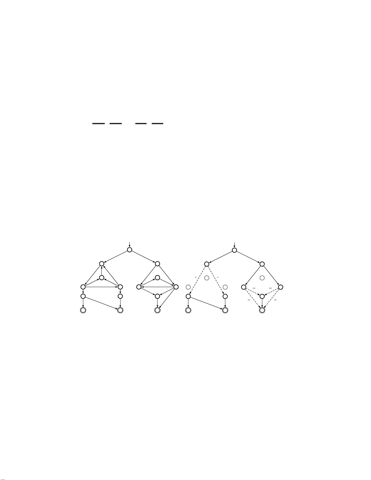
p . W e denote the set of all represe n tative counterexamples to M | = ≤ p ♦ ψ by R ( M , p, ψ ). Theorem 4. 2. L et D b e a MDP , ψ a pr op ositional formula and p ∈ [0 , 1] . If C is a r epr esent ative c ounter example to D | = ≤ p ♦ ψ , then hC i is a c ounter example to D | = ≤ p ♦ ψ . F urthermor e, ther e exists a c ounter example to D | = ≤ p ♦ ψ if and only if ther e exist s a r epr esent ative c ounter example to D | = ≤ p ψ . F o llo wing [HK07a], we present the notions of minimum c ounter example , str ongest evidenc e and m ost indic ative c ounter examples . Definition 4.3 (Minimum counterexample) . Let M b e a MC, ψ a pro positiona l for - m ula and p ∈ [0 , 1]. W e say that C ∈ R ( M , p, ψ ) is a minimum c ounter example if |C | ≤ |C ′ | , for all C ′ ∈ R ( M , p, ψ ). Definition 4 . 4 (Strongest evidence) . Let M b e a MC, ψ a prop ositional formula and p ∈ [0 , 1]. A str ongest evidenc e to M 6| = ≤ p ♦ ψ is a finite path σ ∈ Reach ⋆ ( M , Sat( ψ )) such that Pr M ( h σ i ) ≥ Pr M ( h ρ i ), for all ρ ∈ Reach ⋆ ( M , Sat( ψ )). Definition 4.5 (Most indicative co un terexample) . Let M be a MC, ψ a pr opositiona l formula and p ∈ [0 , 1]. W e ca ll C ∈ R ( M , p, ψ ) a most indic ative c ounter example if it is minim um and Pr ( hC i ) ≥ Pr ( hC ′ i ), for all minimum co unterexamples C ′ ∈ R ( M , p, ψ ). Unfortunately , very often most indicative counterexamples are very lar ge (even infinite), many of its elements hav e insignificant measur e and elements can b e extremely similar to each other (consequently providing the s ame diagnostic information). E v en worse, sometimes the finite pa ths with highes t probability do not exhibit the wa y in which the system accumulates higher pro babilit y to reach the undesired prop erty (and consequently where an er ror o ccurs with hig her probability). F or these reaso ns, we are of the opinion that representative counterexamples a re s till to o general in order to b e useful a s feedback information. W e approach this problem by splitting out the representative counterexample into sets of finite paths following a “ similarit y” criteria (in tro duced in Section 5). These se ts are called witnesses of the c ount er example . Recall that a se t Y of nonempt y sets is a partition of X if the elements of Y cov er X a nd the elements of Y are pairwis e disjoint. W e define co un terexample partitions in the following way . 7 Definition 4 . 6 (Counterexample partitio ns and witnesses) . Let D b e a MDP, ψ a prop ositional for m ula, p ∈ [0 , 1 ], and C a representativ e count er example to D | = ≤ p ♦ ψ . A c ounter example p artition W C is a par tition of C . W e ca ll the elements of W C witnesses . Since not every par tition genera tes useful witnesses (fro m the debugging p ersp ec- tive), we now state prop erties that witnesses must satisfy in order to b e v aluable as diagnostic informatio n. In Sec tio n 7 we show how to partition the detailed counterex- ample in order to obtain useful witness es. Similarity: E le ments o f a witness should provide similar debugging informa tion. Accuracy : Witnesses with higher probability sho uld show evolution of the system with higher proba bility o f containing er rors. Originality: Different witnesses should provide different debugging informatio n. Significance: The pr obabilit y of a witnesses sho uld b e clos e to the probability b ound p . Finiteness : The num b er of witnesses of a co unterexamples partition sho uld b e finite. 5 Rails and T orren ts As ar g ued be fo re we co nsider that representative counterexamples are exces s iv ely gen- eral to b e useful a s feedba ck infor mation. Therefore, we gro up finite paths o f a repr e- sentativ e c o un terexample in witnesses if they are “similar enough” . W e will consider finite paths that b eha ve the same outside SCCs of the system as providing simila r feedback information. In order to for malize this idea , we fir st reduce the origina l Ma rk ov chain to an acyclic one that preser v es r e ac hability probabilities. W e do so by removing all SCCs K of M keeping just input states of K. In this wa y , we get a new ac yclic MC denoted by Ac( M ). The pr o babilit y matrix of the Mar k ov chain relates input s tates of each SCC with its output states with the rea c hability probability b et ween these states in M . Seco ndly , we establish a map b et ween finite pa ths σ in Ac( M ) ( r ails ) and sets of finite paths W σ in M ( torr ents ). Each torrent contains finite paths that are similar, i.e., b ehav e the same outside SCCs. Additionally we show tha t the proba bilit y of σ is equal to the pro babilit y o f W σ . Reduction to Acyclic Mark ov Chains Consider a MC M = ( S, s 0 , P , L ). Rec a ll that a subset K ⊆ S is called str ongly c onne cte d if for every s, t ∈ K ther e is a finite path from s to t . Additionally K is called a str ongly c onne cte d c omp onent (SCC) if it is a maximally (with resp ect to ⊆ ) strongly connected subset of S . Note that every state is a member of exactly one SCC of M (even thos e states that are not inv olved in cycles, since the trivial finite path s connects s to itse lf ). F ro m now on we let SCC ⋆ be the set of non trivia l strong ly connected comp onent s of a MC, i.e., those comp osed o f more than one state. A Markov chain is c alled acyclic if it do es not hav e non triv ia l SCCs. Note that an acyclic Markov chain still ha s abso rbing states. Definition 5.1. Let M = ( S, s 0 , P , L ) b e a MC. Then, for ea c h SCC ⋆ K of M , we define the sets Inp K ⊆ S of all states in K that hav e an incoming trans ition from a state outside of K and Out K ⊆ S o f all sta tes outside of K that have an incoming transition from a state o f K in the following w ay Inp K , { u ∈ K | ∃ s ∈ S \ K . P ( s, u ) > 0 } , Out K , { s ∈ S \ K | ∃ u ∈ K . P ( u, s ) > 0 } . 8 W e also define for each SCC ⋆ K a MC re lated to K a s M K , (K ∪ Out K , s K , P K , L K ) where s K is any state in Inp K , L K ( s ) , L ( s ), and P K ( s, t ) is equal to P ( s, t ) if s ∈ K and equal to 1 s otherwise. Additionally , for every state s inv olved in non triv ial SCCs we define SCC + s as M K , where K is the SCC ⋆ of M such that s ∈ K . Now we are able to define an ac y clic MC Ac( M ) r elated to M . Definition 5.2. Let M = ( S, s 0 , P , L ) be a MC. W e define Ac( M ) , ( S ′ , s 0 , P ′ , L ′ ) where • S ′ , S com z }| { S \ [ K ∈ SCC ⋆ K S S inp z }| { [ K ∈ SCC ⋆ Inp K • L ′ , L | S ′ , • P ′ ( s, t ) ,        P ( s, t ) if s ∈ S com , Pr M ,s (Reach(SCC + s , s, { t } )) if s ∈ S inp ∧ t ∈ Out SCC + s , 1 s if s ∈ S inp ∧ Out SCC + s = ∅ , 0 otherwise. Note that Ac( M ) is indeed a cyclic. Example 2. Cons ide r the MC M o f Figure 5(a). The strong ly connected co mponents of M are K 1 , { s 1 , s 3 , s 4 , s 7 } , K 2 , { s 5 , s 6 , s 8 } a nd the singletons { s 0 } , { s 2 } , { s 9 } , { s 10 } , { s 11 } , { s 12 } , { s 13 } , and { s 14 } . The input states of K 1 are Inp K 1 = { s 1 } and its output s ta tes ar e Out K 1 = { s 9 , s 10 } . F or K 2 , Inp K 2 = { s 5 , s 6 } and Out K 2 = { s 11 , s 14 } . The reduced acyclic MC of M is shown in Figure 5(b). s 0 s 1 s 2 s 3 s 4 s 5 s 6 s 7 s 8 s 9 s 10 s 11 s 12 s 13 s 14 0 , 4 0 , 6 1 0 , 4 0 , 6 0 , 3 0 , 4 0 , 3 0 , 2 0 , 3 0 , 5 0 , 6 .. 0 , 4 . 0 , 3 . 0 , 5 0 , 2 1 .. 1 0 , 2 0 , 8 1 1 (a) Original MC s 0 s 1 s 2 s 5 s 6 s 9 s 10 s 11 s 12 s 13 s 14 s 3 s 4 s 7 s 8 0 , 4 0 , 6 0 , 4 0 , 6 0 , 2 0 , 8 1 1 2 3 1 3 35 41 6 41 35 41 6 41 (b) Derived A cyclic MC Fig. 5: Rails and T orrents W e now r elate (finite) paths in Ac( M ) (rails) to sets o f (finite) paths in M (tor ren ts). Definition 5.3 (Rails) . Let M b e a MC. A finite path σ ∈ Paths ⋆ (Ac( M )) will b e called a r ail of M . Consider a rail σ , i.e., a finite path of Ac( M ). W e will use σ to r epresen t those paths ω of M that behave “similar to ” σ outside SCCs of M . Naively , this means that σ is a subsequence of ω . There a re t wo technical subtleties to deal with: every input state in σ must b e the first s tate in its SCC in ω (freshness) and every SCC visited by ω m ust be also visited b y σ (inertia) (see Definition 5.5). W e need these extra co nditions to make sure that no path ω b ehav es “similar to” tw o distinct rails (see Lemma 5.7). Recall that g iv en a finite sequence σ and a (p ossible infinite) s equence ω , we say that σ is a su bse quenc e o f ω , denoted by σ ⊑ ω , if and only if there exists a strictly incre a sing function f : { 0 , 1 , . . . , | σ | − 1 } → { 0 , 1 , . . . , | ω | − 1 } such that ∀ 0 ≤ i< | σ | .σ i = ω f ( i ) . If ω is an infinite sequence, we in terpr et the codo main o f f a s N . In ca se f is such a function we write σ ⊑ f ω . Note that finite paths and paths are seque nc e s. 9 Definition 5.4. Let M = ( S, s 0 , P , L ) b e a MC. On S we consider the eq uiv alence relation ∼ M satisfying s ∼ M t if and only if s and t are in the same strongly co nnected comp onen t. Again, we usua lly o mit the subsc r ipt M from the no tation. The following definition r efines the notion of subseque nc e , taking car e of the tw o techn ica l subtleties noted above. Definition 5 . 5. Let M = ( S, s 0 , P , L ) b e a MC, ω a (finite) path of M , and σ ∈ Paths ⋆ (Ac( M )) a finite path of Ac( M ). Then we write σ  ω if ther e exis ts f : { 0 , 1 , . . . , | σ | − 1 } → N such that σ ⊑ f ω and for all 0 ≤ i < | σ | we hav e ∀ 0 ≤ j 0 } is the set of states reaching ψ in M . The following theo rem shows the relation b et ween paths, finite paths, a nd pr ob- abilities o f M , M ψ , and Ac( M ψ ). Most imp ortantly , the pro babilit y of a r ail σ (in Ac( M ψ )) is equal to the probability of its as s ociated to rren t (in M ) (item 5 b elo w) and the probability of ♦ ψ is no t affected by reducing M to Ac( M ψ ) (item 6 b elo w). Note that a ra il σ is a lways a finite path in Ac( M ψ ), but that we can talk ab out its asso ciated torrent T or r ( M ψ , σ ) in M ψ and ab out its asso ciated torrent T or r ( M , σ ) in M . The former exists for tec hnical convenience; it is the latter that w e ar e ultimately int er e s ted in. The following theorem also shows that for our purp oses, viz. the definition of the ge nerators of the torrent and the pr o babilit y of the tor ren t, there is no difference (items 3 and 4 b elow) . Theorem 6.2. L et M = ( S, s 0 , P , L ) b e a MC and ψ a pr op ositional formula. Then for every σ ∈ Paths ⋆ ( M ψ ) 1. Rea ch ⋆ ( M ψ , s 0 , Sat( ψ )) = Rea c h ⋆ ( M , s 0 , Sat( ψ )) , 2. Pr M ψ ( h σ i ) = Pr M ( h σ i ) , 3. GenT or r( M ψ , σ ) = GenT or r( M , σ ) , 4. Pr M ψ (T o rr( M ψ , σ )) = Pr M (T o rr( M , σ )) , 5. Pr Ac( M ψ ) ( h σ i ) = Pr M (T o rr( M , σ )) , 6. Ac( M ψ ) | = ≤ p ♦ ψ if and only if M | = ≤ p ♦ ψ , for any p ∈ [0 , 1] . Definition 6. 3 (T orr en t-Counterexamples) . Let M = ( S, s 0 , P , L ) b e a MC, ψ a prop ositional formula, and p ∈ [0 , 1] such that M 6| = ≤ p ♦ ψ . Let C b e a repres en tative counterexample to Ac( M ψ ) | = ≤ p ♦ ψ . W e define the set T o rRepCoun t( C ) , { GenT orr( M , σ ) | σ ∈ C } . W e call the set T orRepCount( C ) a torr ent-c ounter example of C . Note that this s et is a partition of a coun terex a mple to M | = ≤ p ♦ ψ . Additionally , we deno te by R t ( M , p, ψ ) to the set of all to rren t-co unterexamples to M | = ≤ p ♦ ψ , i.e., { T orRepCo un t( C ) | C ∈ R ( M , p, ψ ) } . 11 Theorem 6.4 . L et M = ( S, s 0 , P , L ) b e a MC , ψ a pr op ositional formula, and p ∈ [0 , 1] such that M 6| = ≤ p ♦ ψ . T ake C a r epr esentative c ounter example to Ac( M ψ ) | = ≤ p ♦ ψ . Then the set of finite p aths U W ∈ T orRepCount( C ) W is a r epr esent ative c ounter example to M | = ≤ p ♦ ψ . Note that for each σ ∈ C we get a witness GenT orr( M , σ ). Also note tha t the nu mber of rails is finite, so there are also only finitely ma n y witnesses. F o llo wing [HK0 7a], we extend the notions of m inimum c ounter examples , str ongest evidenc e and s m allest c ounter example to torrents. Definition 6 .5 (Minim um torr en t-counterexample) . Let M be a MC, ψ a prop osi- tional for m ula a nd p ∈ [0 , 1]. W e say that C t ∈ R t ( M , p, ψ ) is a minimum t orr ent- c ounter example if |C t | ≤ |C ′ t | , for all C ′ t ∈ R t ( M , p, ψ ). Definition 6 . 6 (Strongest torrent-evidence) . Let M be a MC, ψ a prop ositional for- m ula and p ∈ [0 , 1]. A stro ngest torr ent- evidenc e to M 6| = ≤ p ♦ ψ is a to rren t W σ ∈ T o rr( M , Sat( ψ )) such that Pr M ( W σ ) ≥ Pr M ( W ρ ) for all W ρ ∈ T o rr( M , Sat( ψ )). Now we define our notio n of significant diagnos tic co unterexamples. It is the gen- eralization of most indicative co un terexample from [HK07 a ] to our setting. Definition 6. 7 (Most indicative tor ren t-counterexample) . Let M b e a MC, ψ a prop o- sitional fo rm ula and p ∈ [0 , 1]. W e call C t ∈ R t ( M , p, ψ ) a most indic ative torr ent- c ounter example if it is a minim um torr e nt-counterexample and Pr ( S W ∈C t h W i ) ≥ Pr ( S W ∈C ′ t h W i ) for all minimum tor ren t counterexamples C ′ t ∈ R t ( M , p, ψ ). By Theo rem 6 .4 it is p ossible to obtain stronges t torr e n t-evidence and most indica- tive torrent-counterexamples o f a MC M by o btaining str ongest evidence and most indicative counterexamples o f Ac( M ψ ) resp ectiv ely . 7 Computing Coun terexamples In this s ection we show how to compute most indicative torrent-count er examples. W e also discus s what information to pres en t to the use r: how to present witness es and how to deal with ov er ly la rge stro ng ly connected comp onen ts. 7.1 Maximizing Sc hedulers The calculation of a maximal probability on a reachabilit y problem can be per formed by solving a linear minimizatio n problem [BdA95,dA97]. This minimization problem is defined on a system of inequalities that has a v ariable x i for each differ e n t state s i and an inequality P j π ( s j ) · x j ≤ x i for each distribution π ∈ τ ( s i ). The maximizing (deterministic memoryles s) scheduler η c an b e easily extra c ted out o f such system of inequalities after obtaining the s olution. If p 0 , . . . , p n are the v alues that minimize P i x i in the pr e vious system, then η is such that, for all s i , η ( s i ) = π whenever P j π ( s j ) · p j = p i . In the following we deno te P s i [ ♦ ψ ] , x i . 7.2 Computing most indi cat i ve torren t-counterexa mpl es W e divide the co mputation of mo st indicative torrent-count er examples to D | = ≤ p ♦ ψ in three stages: pr e-pr o c essing , SCC analysis , and se ar ching . Pre-pro cessing s tage. W e first mo dify the original MC M b y making a ll states in Sat( ψ ) ∪ S \ Sat ♦ ( ψ ) abso rbing. In this wa y we obtain the MC M ψ from Definition 6 .1. Note that we do no t hav e to s p end additional computational resour c es to compute this set, since Sa t ♦ ( ψ ) = { s ∈ S | P s [ ψ ] > 0 } and hence all req uir ed data is already av ailable from the L TL mo del ch ecking phas e. 12 SCC analysis s tage. W e re move all SCCs K of M ψ keeping just input states of K, getting the acyclic MC Ac( M ψ ) according to Definition 5 .2. T o compute this, we first need to find the SCCs of M ψ . Ther e exists well known algorithms to achiev e this: K osara ju’s, T ar jan’s, Gab o w’s algo rithms (among others). W e also hav e to compute the r eac hability pro babilit y from input states to output states of every SCC. This can b e done by using stea dy state a nalysis techniques [Cas 9 3]. Searc hing stage. T o find most indicative torrent-counterexamples in M , we find most indicative counterexamples in Ac( M ψ ). F o r this we us e the same approa c h as [HK07a], turning the MC in to a weigh ted digr aph to exchange the problem of finding the finite path with highest pro babilit y by a s hortest path problem. The no des of the digraph are the states of the MC and there is an edge b et ween s and t if P ( s, t ) > 0. The weigh t of such an edge is − log P ( s, t ). Finding the mo st indicative co un terexample in Ac( M ψ ) is now reduced to finding k sho r test paths. As explained in [HK07a], our algo rithm has to compute k o n the fly . Eppstein’s alg orithm [Epp98] pr oduces the k s hortest paths in gener al in O ( m + n log n + k ), where m is the num b er of no des and n the num ber of edges. In our case, since Ac( M ψ ) is acyclic, the complexity dec r eases to O ( m + k ). 7.3 Debugging i ssues Representa tive finite paths. What we have co mputed so far is a mos t indicative counterexample to Ac( M ψ ) | = ≤ p ♦ ψ . This is a finite set of r a ils, i.e ., a finite set of paths in Ac( M ψ ). E ac h of these pa ths σ repr e sen ts a witness GenT orr( M , σ ). No te tha t this witness itself has usua lly infinitely many elements. In pra ctice, one somehow has to display a witness to the user. The obvious wa y would b e to show the user the r ail σ . This, how ever, may b e confusing to the user as σ is no t a finite path of the original Markov Decision P roces s. Instead o f presenting the user with σ , we therefor e show the user the element o f GenT orr( M , σ ) with highest probability . Definition 7. 1. Let M be a MC, a nd σ ∈ Paths ⋆ (Ac( M ψ )) a ra il of M . W e define the r epr esentant of T orr( M , σ ) as repT orr ( M , σ ) = r e pT orr   ] ρ ∈ GenT orr( M ,σ ) h ρ i   , a rg max ρ ∈ GenT orr( M , σ ) Pr ( h ρ i ) Note that given repT or r ( M , σ ), one can easily recover σ . Therefor e, no information is lost by prese nting torrents as a single element o f the torre nt instea d of as a r a il. Expanding SCC . It is po ssible that the system contains some very lar g e stro ngly connected comp onents. In that case , a single witness co uld have a very lar g e probability mass and one could arg ue that the infor mation presented to the us er is not detailed enough. F or instance, consider the Markov chain o f Figure 6 in w hich ther e is a sing le large SCC with input state t and output state u . K 1 s t u Fig. 6 : The most-indicative tor ren t co un terexample to the prop ert y M | = ≤ 0 . 9 ♦ ψ is simply { GenT or r ( stu ) } , i.e., a sin- gle witness with probability mass 1 asso ciated to the r a il stu . Although this may seem uninfor mativ e, we argue tha t it is more infor mativ e than listing several paths of the form st · · · u with probability summing up to, say , 0 . 91 . Our single witness counterexample suggests that the outgoing edge to a state not rea c hing ψ was simply forgo tten; the listing of paths still allows the p ossibility that one of the probabilities in the who le system is simply wro ng. 13 Nevertheless, if the user needs more informatio n to tackle bugs ins ide stro ngly connected comp onents, note that there is mo re information av a ilable at this p oin t. In particular, for every strongly co nnected comp onen t K, ev ery input state s of K (even for every state in K ), and e v ery output sta te t of K, the proba bilit y of reaching t from s is already av aila ble from the computation of Ac( M ψ ) during the SCC analysis stage of Section 7.2. 8 Final Discussion W e have presented a nov el technique for r epresent ing a nd co mputing co un terexamples for nondeterministic and probabilistic sys tems. W e pa rtition a counterexample in wit- nesses and state five prop erties that w e believe go o d witness es should sa tisfy in or der to b e useful as debugg ing to ol: (simila rit y) elements o f a witness should provide simila r debugging infor mation; (origina lit y) different witnesses s hould provide different debug- ging information; (a ccuracy) witnesses with higher pro babilit y should indicate system behavior more likely to contain err ors; (sig nificance) pro babilit y of a witness should be relatively high; (finiteness ) there should b e finitely many witnesses. W e achiev e this by gr ouping finite paths in a coun tere xample together in a witness if they behave the same outside the strong ly connected comp onent s. Presently , some work has b een done on counterexample genera tio n techniques for different v aria n ts of probabilistic mo dels (Discrete Markov chains and Con tinues Marko v chains) [AHL05,AL06,HK07 a ,HK07 b ]. In o ur ter mino logy , these works consider wit- nesses consis ting of a single finite path. W e hav e alr eady discussed in the Intro duction that the single path approach do es not meet the prop erties of a ccuracy , originality , significance, and finiteness. Instead, our witness/ torrent approach provides a high level of abstraction of a coun- terexample. By g rouping together finite paths that b eha ve the same outside strongly connected comp onen ts in a single witness, w e can achiev e these prop erties to a higher extent. Behaving the s a me outside str ongly connected co mponents is a r easonable wa y of for malizing the concept of providing similar debugging information. This gr ouping also makes witnesses significantly different form each other: each witness co mes form a different rail and each rail provides a differen t wa y to reach the undesired pr o perty . Then ea ch witness provides original information. Of co urse, our witnesse s are more sig- nific ant than single finite paths, b ecause they are s e ts of finite paths. This a lso gives us more ac cur acy than the approa c h with single finite paths, as a collection of finite paths behaving the s ame a nd r eac hing an undesired c ondition w ith high proba bilit y is more likely to show ho w the system reaches this c o ndition than just a single path. Finally , bec ause there is a finite num b er of rails, there is a lso a fin ite num b er of witnes ses. Another key difference of our work to prev ious ones is that our tec hnique allows us to generate counterexamples for probabilistic systems with nondeterminis m. How ever, a recent rep ort [AL07] also consider s counterexample generatio n for MDPs. This work is limited to upp er b ounded pCTL formulas without nested temp oral op erators . Besides, their technique significa n tly differs from ours . Finally , among the r elated work, we would like to str ess the res ult of [HK07a], which provides a sy stematic characterization of co un terexample genera tion in terms of shortest paths pro ble ms . W e use this result to gener ate counterexamples for the acyclic Marko v Cha ins. In the future we intend to implement a to ol to generate our significant diagnostic counterexamples; a very preliminary version has alrea dy b een implemented. There is still work to b e done on improving the v isualization of the witnesses, in particular, when a witness captures a lar ge strongly connected comp onen t. Another direction is to investigate how this work can b e ex tended to timed systems, e ither mo deled with contin uous time Markov chains or with probabilistic timed automata. 14 References AHL05. Husain A lj azzar, Holger Hermanns, and Stefan Leue. Counterexamples for timed probabilistic reachabili ty . In F ormal Mo deling and Analysis of Time d Systems (F ORMA TS ’05) , volume 3829, pages 177–195, 2005. AL06. Husain A lj azzar and S tefa n Leue. Extended directed search for probabilistic timed reac hability . In F ormal Mo deling and Analysis of Tim e d Systems (FORMA TS ’06) , pages 33–51, 2006. AL07. Husain Aljazzar and Stefan Leue. Coun terexamp les for mo del chec king of marko v decision pro cesses. Computer Science T echnical Rep ort soft-08-01, Un iv ersity of Konstanz, December 2007. BdA95. Andrea Bianco and Luca de Alfaro. Model checking of probabilistic and non- deterministic sy stems. In G. Go os, J. Hartmanis, and J. v an Leeuw en, editors, F oundations of Softwar e T e chnolo gy and The or etic al Computer Scienc e (FSTTCS ’95) , volume 1026, pages 499–513, 1995. Bel57. Ric hard E. Bellman. A Marko vian decision pro cess. J. Math. M e ch. , 6:679–684, 1957. BLR05. Gerd Behrmann, Kim G. Larsen, and Jacob I. Rasmussen. Optimal scheduling using priced t imed automata. SIGMETRICS Perform. Eval. R ev. , 32(4):34–4 0, 2005. Cas93. Christos G. Cassandras. Di scr ete Event Systems: Mo deling and Performanc e Ana l- ysis . R ic hard D. Irwin, Inc., and Ak sen Asso ciates , I nc., 1993. CGJ + 00. Edmund M. Clark e, Orna Grumberg, Somesh Jha, Y uan Lu, and Helmut V eith. Countere x amp le-guided abstraction refinement. In Computer Aide d V erific ation , pages 154–169, 2000. dA97. Luca de Alfaro. F ormal V erific ation of Pr ob abil istic Systems . PhD thesis, Stanford Universit y , 1997. dAKM97. Luca de Alfaro, Arjun Kapur, and Zohar Manna. H ybrid diagrams: A deductive- algorithmic approac h to hybrid system verification. In Symp osium on The or etic al Asp e cts of Computer Scienc e , pages 153–164, 1997. Epp98. David Eppstein. Finding the k shortest paths. In SI AM Journal of C omput i ng , pages 652–673, 1998. FV97. J. Filar and K. V rieze. Comp etitive Markov De cision Pr o c esses . 1997. HK07a. T ingting Han and Jo ost-Pieter Kato en. Coun terexamples in probabilistic mo del chec king. In T o ol s and Algorithms f or the Construct ion and Analysis of Systems: 13th International Confer enc e (T ACAS ’ 07) , vol ume 4424, pages 60–75, 2007. HK07b. Tingting Han and Joost-Pieter Kato en. Pro viding evidence of likely b eing on time counterexample generation for ctmc mo del chec king. In International Symp osium on Automate d T e chnolo gy f or V erific ation and Analysis (A TV A ’ 07) , volume 4762, pages 331–346, 2007. MP91. Z. Manna an d A. Pnueli. The T emp or al L o gic of R e active and Concurr ent Systems: Sp e cific ation . S pringer, 1991. PZ93. Amir Pnueli and Lenore D. Zuck. Probabilistic verification. Information and Computation , 103(1):1–29, 1993. SdV04. Ana S ok olo v a and Erik P . de Vink. Probabilistic automata: System types, parallel composition and comparison. I n Christel Baier, Boudewijn R. H averk ort, Holger Hermans, Jo ost-Pieter Kato en, and Markus Siegle, editors, V al idation of Sto chastic Systems: A Guide to Curr ent R ese ar ch , volume 2925, pages 1–43. 2004. SL95. Rob erto Segala and Nancy Ly nc h. Probabilistic sim ulations for probabilistic pro- cesses. Nor dic Journal of Computing , 2(2):250–273 , 1995. V ar85. M.Y. V ardi. Aut oma tic verification of probabilistic concurrent finite-state systems. In Pr o c. 26th IEEE Symp. F ound. C omp. Sci. , pages 327–338, 1985. 15 App endix: Pro ofs In this app endix we give pro ofs of the results tha t were omitted from the pap e r for space reaso ns. Observ atio n 8.1. L et M b e a MC . Sinc e Ac( M ) is acyclic we have σ i 6∼ σ j for every σ ∈ Paths ⋆ (Ac( M )) and i 6 = j (with the exc eption of absorbing s tates). Observ atio n 8.2. L et σ, ω and f b e such that σ  f ω . Then ∀ i : ∃ j : ω i ∼ σ j . This fol lows fr om σ ⊑ f ω and the inert ia pr op erty. Lemma 8 .3. L et M b e a MC , and σ ts ∈ Paths ⋆ (Ac( M )) . Ad ditional ly let ∆ σts , { ρ tail( π ) | ρ ∈ GenT or r ( σ t ) , π ∈ Paths ⋆ (SCC + t , t, { s } ) } . Then ∆ σts = GenT o r r( σts ) . Pr o of. . ( ⊇ ) Let ρ 0 ρ 1 · · · ρ k ∈ GenT orr( σ ts ) and n t the low est s ubindex of ρ such that ρ n t = t . T a k e ρ , ρ 0 ρ 1 · · · ρ n t and π , ρ n t · · · ρ k (Note tha t ρ 0 ρ 1 · · · ρ k = ρ tail( π )). In order to prov e that ρ 0 ρ 1 · · · ρ k ∈ ∆ σts we need to prov e that (1) ρ ∈ Ge nT o r r( σt ), and (2) π ∈ Paths ⋆ (SCC + t , t, { s } ). (1) Let f b e such that σ ts  f ρ 0 ρ 1 · · · ρ k and f ( | σ ts | − 1) = k . T a k e g : { 0 , 1 , . . . , | σ t | − 1 } → N b e the restr iction of f . It is easy to ch eck that σ t  g ρ . Additionally f ( | σ t | − 1) = n t (otherwise f w ould not satisfy the fr eshness prop ert y for i = | σ t | − 1). Then, by definition of g , we have g ( | σt | − 1) = n t . (2) It is clear that π is a path from t to s . Ther e fore we only hav e to show that every state of π is in SCC + t . By definition of SCC + t , π 0 = t ∈ SCC + t and s ∈ SCC + t since s ∈ Out SCC + t . Additionally , since f satisfies inertia prop erty we have that ∀ f ( | σ t |− 1)