Global sensitivity analysis of computer models with functional inputs

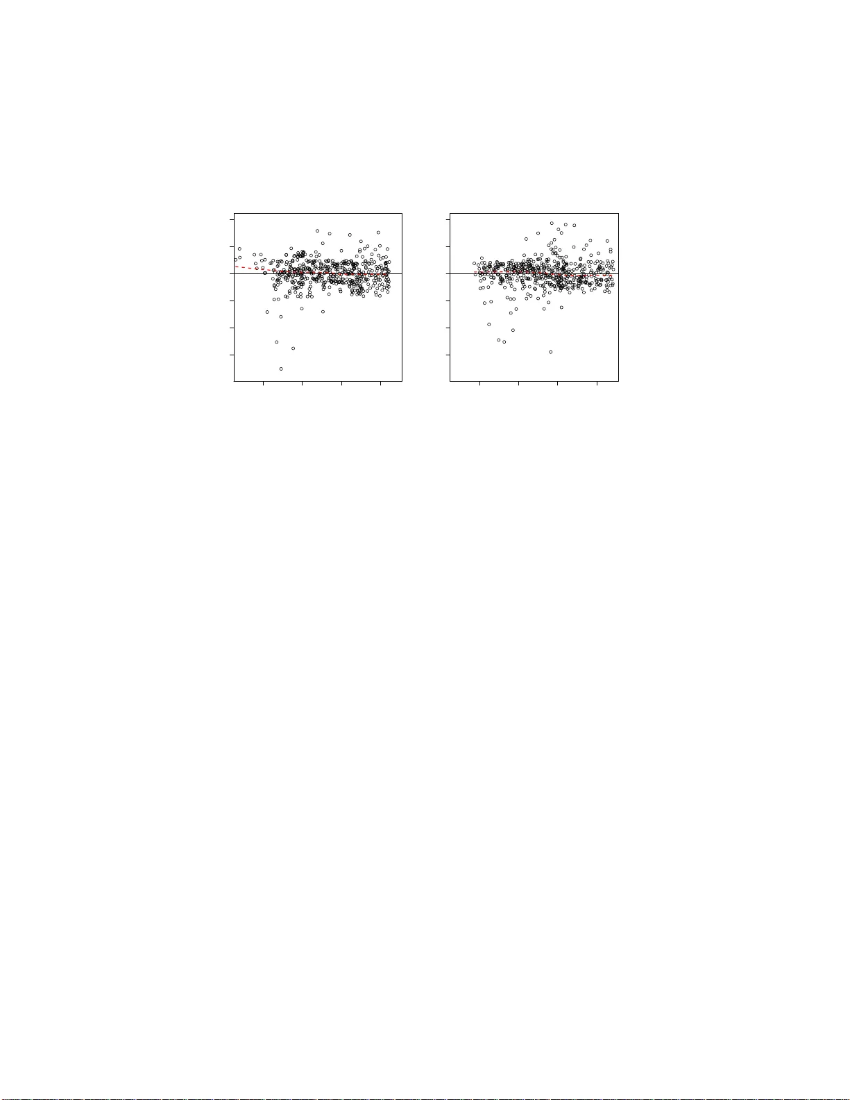
Global sensit ivit y analysis o f computer mo de ls with functional inputs Bertrand IOOSS ∗ and Mathieu RIBA TET † Submitted to: R eliability Engine ering and Syst em Safety for the sp ecial SAMO 200 7 issue ∗ CEA, DEN, DER/SESI/LCFR, F-13 108 Sain t-P aul-lez-Durance, F rance. † ´ Ecole P olytec hniqu e F ´ ed ´ erale de Lausanne, Chair of Statistics, ST A T-IMA-FSB-EPFL, Station 8, CH-1015 Lausanne, Switzerland. Corresp onding author: B. Io oss ; Email: b ertrand.io oss@ cea.fr Phone: +33 (0)4 42 25 72 73 ; F ax: +33 (0)4 42 25 24 08 Abstract Global sensitivity analysis is used to quantify the influence of uncertain input parame- ters o n the resp onse v ariability of a numerical mode l. The c o mmon qua nt itative methods are a ppropriate with computer co des ha ving sca lar input v aria bles. This pa pe r aims at illustrating different v ariance-base d sensitivity analysis techniques, bas ed on the so -called Sob ol’s indices , when s ome input v ariables a re functional, such as sto chastic pro cesse s or random spa tial fields. In this w ork , we fo c us on lar ge cpu time computer co des which need a preliminary metamo deling step before p erforming the s ensitivity analysis . W e prop ose the use of the join t mo deling approach, i.e., mode ling sim ultaneously the mea n and the disp e rsion of the code outputs using t wo interlink ed Gener a lized Linear Mo dels (GLM) or Gener alized Additive Mo dels (GAM). The “mean mo del” a llows to estimate the s ensi- tivit y in dices of ea ch sca lar input v ariables, while the “dispe rsion mo del” allows to deriv e the total sensitivity index of the functional input v a riables. The prop ose d approach is compared to s ome classical se ns itivit y analy sis methodolo gies on an a nalytical function. Lastly , the new metho dolog y is applied to an industrial computer co de that simulates the nu clear fuel ir radiation. Keyw ords: Sob ol’s indices, join t modeling, generalized additiv e mo del, metamodel, sto chastic pro cess, uncerta int y 1 1 INTR ODUCTION Mo dern computer codes t hat sim ulate physical phenomenas often tak e as inputs a high nu mber of n umerical para meters and ph ysical v ariables, and return several outputs - scalars or functions. F or the developmen t and the use of such co mputer models, Sensitivity Analysis (SA) is an in v aluable to ol. The orig inal tec hnique, based o n the deriv ative computations o f the mo del outputs with resp ect t o the mo del inpu ts, suffers fro m stro ng limitations for computer mo dels simulating non-linear phenomena. More recent global SA tec hniques tak e in to account the entire ra nge of v ariation of the input s and aim to app ortion the whole output uncer taint y to the input factor uncertaint ies (Saltelli et al. [21]). The global SA metho ds can a lso b e used for mo del calibration, mo del v alidation, decision making pro cess , i.e., any proces s wher e it is useful to know whic h are the v ariables that mo s tly contribute to the output v ariability . The common quantitative methods are applicable to computer codes with scalar input v ariables. F or example, in the n uclear engineering do main, global SA to ols hav e be e n applied to numerous mo dels where a ll the unce r tain input parameters are modele d by random v ariables, p os s ibly co r related - such as ther ma l-hydraulic s ystem co des (Marqu` es et al. [13]), w aste storage safety studies (Helton et a l. [7]), environment al model of dose calculations (Ioo s s et al. [1 0]), reactor dosimetry proce s ses (Ja cques et al. [11]). Recent resear ch pap ers have tried to consider more complex input v ariables in the global SA pro cess, esp ecia lly in petroleum and environmental studies: • T a r antola et al. [27] w ork on an en vironmental asse ssment on soil models that use spatially distr ibuted maps affected by r andom err ors. This kind o f uncerta int y is mo deled by a spatia l random field (following a sp ecified proba bilit y distribution), simulated at eac h co de r un. F o r the SA, the authors pr op ose t o replace the spatial input par a meter b y a “trigger” random parameter ξ that g overns the rando m field simulation. F or some v alues of ξ , the random field is simulated and for the other v alues, the random field v alues a re put to zero. Therefore, the s ensitivity index of ξ is us ed to q uantif y t he influence of the spatial input parameter. • Ruffo et al. [18] ev aluate an oil reservoir pr o duction using a mo del that dep ends on different heterog eneous geolog ical media sce na rios. These scenario s, whic h are of limited num b er, are then substituted for a discrete fac to r (a scenario num b er) before per forming t he SA. 2 • Io o ss et al. [9 ] study a groundwater ra dionuclide migration mo del which dep end on several ra ndom s calar par ameters a nd on a spa tial r andom field (a geos ta tisti- cal simulation of the h ydrogeo logical la yer heter ogeneity). The authors prop ose to consider the spa tia l input pa rameter as a n “uncont ro lla ble” parameter. Therefore, they fit on a f ew s im ulation r e s ults of the co mputer mo del a double mo del, called a joint model: the firs t comp onent models the effects of the scala r parameters while the sec ond mo dels the effects of the “uncontrollable” p ar ameter. In this pap er , we tackle the pro blem of the global SA for numerical mo dels and when some input parameters ε are functional. ε ( u ) is a one o r multi-dimensional sto chastic function w he r e u can b e spatial co o rdinates, time scale or any other physical par ameters. Our w or k fo cuses o n mo dels that dep end on scalar par ameter vector X and inv olve so me sto chastic pro cess sim ulations or random fields ε ( u ) a s input pa rameters. The computer co de output Y depends on the realiza tions of these ra ndom f unctions. These models are t ypically non linear with strong in teractio ns b etw een input parameter s. Therefor e, we concentrate o ur metho dolog y on the v a riance based se ns itivit y indices estimation; that is , the so -called Sob ol’s indices (Sobo l [25], Saltelli et al. [21]). T o deal with this situatio n, a fir st natural appro ach cons ists in using either all the discretized v a lues o f the input functional par a meter ε ( u ) or its decomp osition into an appropria te basis of o rthogona l functions. The n, for a ll the new scalar parameter s r e lated to ε ( u ), s ensitivity indices a re computed. How ever, in the case of complex functiona l parameters , this approa ch seems to b e ra pidly intractable as these parameters cannot be repres ented by a small num ber of scalar par ameters (T a rantola et al. [2 7]). Mo re- ov er, when dealing with non physical parameters (for example co efficients of orthogonal functions used in the decomposition), sensitivity indices interpretation may be labor io us. Indeed, most o ften, ph ysicists w ould pr e fer t o obtain one globa l sensitivit y index rela ted to ε ( u ). Fina lly , a m a jor drawback for the decomp os itio n a pproach is related to the un- certaint y modeling stage. Mor e precisely , this a pproach needs to sp ecify the probability density functions for the coefficients of the decomp ositio n. The following section presents three different strateg ies to co mpute the Sob ol’s in- dices with functiona l inputs: (a) the macropar ameter metho d, (b) the “trigger ” parameter metho d a nd (c) the propos ed joint mo deling appr oach. Sectio n 3 compar es the relev ance of these three stra tegies on an analytical example: the WN-Ishigami function. Lastly , the prop osed approach is illustrated on an industrial computer co de simulating fuel irradiation 3 in a n uclear rea ctor. 2 COMPUT A TIONAL MET HODS OF S OBOL’S IN- DICES First, let us reca ll s o me basic notions a bo ut So b o l’s indices. Let define the mo del f : R p → R X 7→ Y = f ( X ) (1) where Y is the co de output, X = ( X 1 , . . . , X p ) ar e p indep endent inputs, and f is the mo del function. f is considered as a “ black b ox” , i.e. a function whose analytical formula- tion is unknown. The main idea of the v ariance-based SA metho ds is to ev aluate how the v ariance of an input or a group o f input para meters contributes to the output v ariance of f . These con tributions are descr ib ed using th e follo wing sensitivity indices: S i = V ar [ E ( Y | X i )] V ar( Y ) , S ij = V ar [ E ( Y | X i X j )] V ar( Y ) − S i − S j , S ij k = . . . (2) These coefficients, na mely the Sob ol’s indices, c an be used for an y c o mplex mo de l functions f . The s econd or der index S ij expresses the model sens itivity to the in teraction b etw een the v ariables X i and X j (without the first order effects of X i and X j ), a nd so on for higher orders effects. The in terpretation of these indices is natur al as all indices lie in [0 , 1] and their sum is equal t o one. The larger an index v alue is, the greater is the imp ortance of the v ariable or the gro up of v ariables rela ted to this index. F or a mo del with p inputs, the num be r of Sob ol’s indices is 2 p − 1; leading to an int rac ta ble n um b er of indices as p increases . Thus, to express the ov erall output sensitivit y to a n input X i , Homma & Saltelli [8 ] in tro duce the to ta l s ensitivity index: S T i = S i + X j 6 = i S ij + X j 6 = i,k 6 = i,j 1000, i.e. more tha n thousand model ev a luations for one input parameter (Saltelli et al. [22]). In c o mplex industrial applicatio ns, this a pproach is in tracta ble due to the c pu time co st of o ne mo del ev aluation and the poss ible large num ber of input parameters. 6 2.2 The “t rigger” parameter metho d Dealing with spatially distributed input v ariables , T a rantola e t al. [27] pro p o se an alter- native that us es an additional scalar input parameter ξ - called the “trigger” parameter. ξ ∼ U [0 , 1] gov erns the random function simulation. Mo re precisely , for each simulation, if ξ < 0 . 5, the functional pa rameter ε ( u ) is fixed to a nominal v alue ε 0 ( u ) (for example the mean E [ ε ( u )]), while if ξ > 0 . 5 , the functional pa rameter ε ( u ) is simulated. Using this metho dology , it is poss ible to es timate how sensitive the mo del output is t o th e presence of the random function. T ara nt ola et al. [27] use the Ex tended F AST metho d to co m- pute the first order and total sensitivity indices of 6 scalar input fac to rs and 2 additional “trigger ” para meters. F or their study , the sensitivity indices accor ding to the “ trigger ” pa- rameters a re small and the authors co nclude that it is unnecessary to mo del these spatial error s mor e accur ately . Contrary to the prev ious metho d, there is no restrictio n about the sens itiv ity indices estimation pro cedure - i.e. Monte-Carlo, F AST, quas i Mo nte-Carlo. How ever, ther e are t wo ma jor dr awbac ks for this approach: • As the macropa rameter method, it als o requires the use of the computer mo del to per form the SA and it may be problematic for larg e cpu time computer mo dels. This problem c an b e comp ensated by the use of an efficient quasi Mo nt e-Car lo algorithm for which the s ampling desig n size can b e decreased to N = 10 0. • As underlined by T arantola et al. [27], ξ reflects only the presence or the absence of the sto chastic errors on ε 0 ( u ). There fo re, the ter m V ar[ E ( Y | ξ )] do es no t qua nt ify the contribution of the r andom function v ariability to the o utput v ariabilit y V ar ( Y ). W e will discuss ab out the significa nce of V ar [ E ( Y | ξ )] later, during our a nalytical function a pplica tion. 2.3 The join t mo deling approac h T o p er form a v ariance-based SA for time consuming computer mo dels , some authors pro - po se to approximate the c omputer co de, starting from an initial small-size sampling design, by a mathematical function often called r esp onse surface or metamodel (Marseguerr a et al. [14], V olko v a et a l. [28], F ang et a l. [3]). This metamo del, requiring negligible c pu time, is then used to e s timate Sobo l’s indices b y any method, for example the simple Mo nte-Carlo algorithm. F or metamo dels with sufficient prediction capa bilities, the bias b etw een the 7 exact Sob o l’s indices (from the computer co de) and the Sobol’s indices estimated via the metamo del is negligible. Indeed, it has be e n sho wn that the unexplained v ariance part of the computer co de by the metamo del (which can be measure d) corresp onds to this bias (Sob o l [2 6]). Several choices of metamo del ca n b e found in the literature: p o ly nomials, splines, Ga ussian pr o cesses, neura l netw ork s , . . . The fitting pro ce s s is often bas e d on least squares regres sion techniques. Thus, for the functional inp ut problem, one strategy may b e to fit a metamodel with a m ulti-dimensional sca lar parameters repre senting ε ( u ) as an input parameter - i.e. its discr etization or its decomp osition into an appro priate basis. This pr o cess would corr esp ond to a metamo deling a pproach for the macro parame- ter metho d. How ev er, this appr oach seems to be impracticable due to the potential lar ge nu mber o f scala r parameters: applying reg ression techniques supposes to hav e more obser- v ation p o int s (sim ulation sets) than inpu t parameter s and imp o rtant numerical problem (like matrix conditioning) might o ccur while dealing with co r related input parameters. A second option is to substitute ea ch random function realizatio n for a discr e te num b er, which can corr esp ond to the s cenario par ameter of Ruffo e t al. [18] (where the num ber of geo statistical r ealizations is finite and fixed, and where each different v alue of the discrete par ameter corr esp onds to a different realiza tion). Then, a metamo del is fitted using this dicrete pa rameter as a qua litative input v ariable. How ever, using a metamo del is in teresting when only a few runs of the code is av ailable , which correp o nds to a more limited n umber of realizatio ns o f the functional input. This r estriction o f the po ssible realizations of the input r andom function to a few ones is not appr opriate in a ge ne r al context. Another strategy considers ε ( u ) as an uncon trollable parameter. A metamo del is fitted in function of the o ther sca lar para meters X : Y m ( X ) = E ( Y | X ) (7) Therefore, using the relation V ar( Y ) = V ar[ E ( Y | X )] + E [V ar( Y | X )] (8) it can be easily sho wn that the sensitivity indices of Y g iven the scalar parameters X = ( X i ) i =1 ...p write (Io os s et a l. [9]) 8 S i = V ar[ E ( Y m | X i )] V ar( Y ) , S ij = V ar[ E ( Y m | X i X j )] V ar( Y ) − S i − S j , . . . (9) and can b e co mputed by classical Monte-Carlo techniques applied on the metamo del Y m . Therefore , using equation (8), the total se ns itivity index of Y a c cording to ε ( u ) corres p o nds to the exp ectatio n of the unexpla ined part of V ar ( Y ) b y the metamo del Y m : S T ε = E [V ar( Y | X )] V ar( Y ) (10) Using this appr oach, o ur ob jective is a lter ed b eca use it is impo ssible to decomp os e the ε effects into an e le mentary effect ( S ε ) as well as the interaction effects b etw een ε and the scalar pa rameters ( X i ) i =1 ...p . How ever, we see below that o ur tec hnique allows a qualitative appraisal of the interaction indices. The sensitivity index estimatio ns from equations (9) and (10) r aise tw o difficulties: 1. It is w ell known that classical parametric metamodels (bas e d on least squares fitting) are not adapted to estimate E ( Y | X ) accurately due to the presence of heteroscedas - ticit y (induced b y the e ffect of ε ). Such ca ses are a na lyzed b y Iooss et al. [9]. The authors show that heteros cedasticity may lead to sensitivity indice s missp ecifica- tions. 2. Cla s sical no n pa rametric methods, such as Generalized Additive Mo dels (Hastie and Tibs hirani [6]) a nd Gaus s ian pro c e sses (Sacks et al. [19]) that can provide efficient estimation of E ( Y | X ) (exa mples a re given in Io os s e t a l. [9 ]), ev en in high dimensio nal input cas e s ( p > 5). How ev er, these a pproaches a re base d on a homoscedasticity h yp othesis a nd do not ena ble the estimation of V a r( Y | X ). T o solve the second pro blem, Zaba lza-Mezgha ni et al. [30] prop os e the use of a theory developed for e x pe rimental data (McCulla gh and Nelder [15]): the simultaneous fitting of the mean a nd the disp ersio n by t wo in terlinked Gener a lized Linear Mo dels (GLM), which is called the joint mo deling (see Appendix A.1). Besides, to reso lve the first problem, this approa ch ha s b een extended b y Io oss et al. [9] to non parametr ic mo dels . This generaliza tion allows more complexity and flexibility . The a uthors prop o se the use of Generalized Additive Mo dels (GAMs) bas ed on p ena lized smo othing splines (W o o d [29]). A succint descriptio n of GAM and joint GAM is given in App endix A.2. GAMs allow mo del and v ariable s elections using qua si-likelihoo d function, statistica l tes ts on co effi- 9 cients and gra phical display . How ever, co mpared to other complex metamo dels, GAMs impo se an additive effects h ypothesis . Therefore, tw o metamodels ar e obtained: one for the mean comp onent Y m ( X ) = E ( Y | X ); and the other one for the disp er s ion co mpo nent Y d ( X ) = V ar( Y | X ). The sens itivity indices of X a re co mputed using Y m with the stan- dard proc e dure (Eq. (9 )), while the total sensitivity index of ε ( u ) is computed from E ( Y d ) (Eq. (10)). Using the model for Y d as w ell as the asso ciated regression diagnostics, it is po ssible to deduce q ualitative sensitivity indices for the interactions betw een ε ( u ) and the scalar pa r ameters of X . One ma jor as sumption of the join t modeling a pproach is that the “mean r esp onse” of the co mputer co de is well handled using Y m . Conse quently , all the unexplaine d par t of the computer mo del b y t his metamodel is due to the uncon trolla ble par a meter. In other words, the better the mean comp onent metamodel is, the sma ller is the influence of the uncontrollable parameter. This is a stro ng assumption which ha s to be v alidated in order to av oid err oneous results. In fact, some simple statistical and graphical to o ls can be use d while fitting the mean comp onent (Io oss et al. [9]): the explained deviance v alue, the observed resp onses versus predicted v alues plo t (and its quantile-quant ile plo t) and the deviance residuals plot. This la st plot allows to detect some fitting pr oblems by revealing po ssible biases or lar ge r esidual v alues. Some examples ar e g iven in section 3.2. Thes e to ols can also be applied for the disp ers ion comp onent fit. F or a detailed ov erview of thes e diagnostic to ols , one can r efer to McCullagh & Nelder [15]. 3 APPLICA TION TO AN ANA L YTICAL E XAM PLE The thr e e pr eviously pro po sed metho ds are first illustrated on a simple ana lytical mo del with tw o s calar input v aria bles and o ne functional input: Y = f ( X 1 , X 2 , ε ( t )) = sin( X 1 ) + 7 sin( X 2 ) 2 + 0 . 1[max t ( ε ( t ))] 4 sin( X 1 ) (11) where X i ∼ U [ − π ; π ] for i = 1 , 2 and ε ( t ) is a white noise, i.e. an i.i.d. sto chastic pro - cess ε ( t ) ∼ N (0 , 1 ). In our mo del simulations, ε ( t ) is dis c retized in one hundred v alues : t = 1 . . . 1 0 0. The function (11) is similar to the well-known Ishiga mi function (Homma and Saltelli [8]) but substitute t he third parameter for the maxim um o f a s to chastic pro- cess. Consequently , w e ca ll our function the white-noise Ishigami function (WN-Ishigami). 10 Although the WN-Ishigami function is an analytical mo del, the in tro duction of the maxi- m um of a sto chastic pro cess inside a mo del is quite realis tic. F or exa mple, some computer mo dels simulating physical phenomena c a n use the maximum of time-dep endent v ariable - river height, r ainfall qua ntit y , temp era ture. Such input v ariable ca n b e mo deled by a tempo ral s to chastic pro ces s. As for th e Ishigami function, w e can immedia tely deduce from t he fo r mula (1 1): S ε = S 12 = S 2 ε = S 12 ε = 0 (12) Then, we hav e S T 1 = S 1 + S 1 ε , S T 2 = S 2 , S T ε = S 1 ε (13) In the follo wing, we fo cus our attention on the es tima tion of S 1 , S 2 and S T ε . Because of a particular ly complex probability distribution of the maximum o f a white noise, there is no ana ly tical solution for the theor etical Sob ol’s indices S 1 , S 2 and S T ε for the WN-Ishigami function. E ven with the asymptotic h yp othesis (num b er of time steps tending to infinit y), where the maxim um o f the white noise f ollows Genera lized Extr eme V alue distribution, theoretical indices ar e unrea chable. Therefore, our b enchmark Sob ol’s indices v alues ar e derived from t he Mo nte-Carlo method. 3.1 The macroparameter and “trigger” parameter metho ds T able 1 contains the Sobol’s index es tima tes using the macropa rameter and “trig ger” parameter metho ds. As explained b efore, w e can o nly use s o me algo rithms ba sed on independent Monte-Carlo sa mples . W e apply the algorithm of Sobol [24] that computes S 1 , S 2 , S 1 ε at a cost n = 4 N and the algorithm of Sa ltelli [20] whic h computes the first order indices S 1 , S 2 and the tota l sensitivity indices S T 1 , S T 2 , S T ε at a cost n = 5 N (wher e N is the size of the Monte-Carlo samples, cf. section 2.1). F or the es timation, the size of the Monte-Carlo sa mples is limited to N = 1000 0 b ecause of memo ry co mputer limit. Indeed, the functional input ε ( u ) con tains for ea ch simulation set 10 0 v alues. Then, the input sa mple matrix ha s the dimensio n N × 102 which b ecomes extremely large when N increases. T o ev aluate the effect of t his limited Monte-Carlo sample size N , each Sob ol’s index estimate is asso c iated to a s ta ndard-devia tio n estimated by bo o ts tr ap (Saltelli et al. [22]) - with 10 0 replicates of the input-output sample. The obtained standard-devia tions 11 ( sd ) ar e rela tively small, of the order of 0 . 01, which is r a ther sufficient for o ur exer cise. R emark: We have also trie d to estimate Sob ol’s indic es with sm al ler Monte-Carlo sample sizes N . The or der of the obtaine d standar d-deviations (estimate d by b o otstr ap) of the Sob ol’s estimates a r e the fol lowing: sd ∼ 0 . 0 2 for N = 5 000 , sd ∼ 0 . 04 for N = 100 0 and sd ∼ 0 . 06 for N = 50 0 . We c onclude t hat the Monte-Carlo estimates a r e sufficiently ac cur ate for N > 5 000 . [T able 1 about her e.] Macroparameter F or the macroparameter m etho d, the theoretical rela tions betw een indices giv en in ( 13 ) are satisfied. W e a re therefore confident with the estimates obtained with this metho d and we choo se the S ob ol’s indices obtained with Saltelli’s algor ithm a s the reference indices: S 1 = 55 . 1% , S 2 = 2 0 . 7% , S T ε = 2 4 . 8% The S ε , S 12 , S 2 ε and S 12 ε indices (Eq. (12)) a re not repo rted in table 1 as estimates are negligible. T rig ger parameter Using the “trigger” parameter metho d, the estima tes repor ted in table 1 are quite far from the reference v a lues. The inadequacies are larger than 30% for all t he indices , and can b e larger than 60% for a few one s ( S 2 and S T 2 ). Moreov er, the relations given in (13) are not sa tisfied at all. Actually , replacing the input parameter ε ( u ) by ξ which gov erns the presence or the a bsence o f the functional input parameter changes the mo del. When ε is not simulated, it is replaced by its mean (zero) and the WN-Ishig ami function b eco mes Y = sin( X 1 ) + 7 sin( X 2 ) 2 . Therefore, the mix of the WN-Ishigami mo del and this new mo del p erturbs the estimation of the sensitivity indices, even those unrela ted to ε (like X 2 ). In conclusio n, the o btained results are in concordance with t he expected r esults. This result confirms our exp ectation: sensitivity indices derived fro m the “trigger” parameter metho d have not the sa me sense that the classica l ones, i.e., the mea sure of the contribution of the input parameter v ariability to the output v ariable v ariability . The sensitivity indices obtained with these tw o metho ds ar e unconnec ted because the “trigge r ” parameter metho d c hanges the structure of the model. 12 3.2 The join t mo deling approac h W e apply now the joint mo deling appr o ach whic h requires an initial input-output sample to fit the joint metamodel - the mean comp onent Y m and the disp ersion comp onent Y d . F or our a pplication, a learning sample size o f n = 500 was cons ide r ed; i.e., n indep endent random samples of ( X 1 , X 2 , ε ( u )) were sim ulated leading to n obser v ations for Y . Joint GLM and joint GAM fitting pro cedur es a re fully descr ib ed in Io oss et al. [9]. Some graphical residual analys es are particular ly useful to check the relev ance of the mean and disp e rsion co mpo nents of the jo int mo dels. In the following, we give the results of the joint mo dels fitting o n a learning sample ( X 1 , X 2 , ε ( u ) , Y ). Let us r ecall that we fit a mo del to predict Y in function of ( X 1 , X 2 ). Join t GLM fitting F or the joint GLM, a fourth order po lynomial for the parametr ic form of the mo del is consider ed. Moreover, only the explanato r y terms are retained in o ur regr e ssion mo del using analys is o f deviance and the Fisher statistics. The equa tion of the mean comp onent writes: Y m = 1 . 77 + 4 . 75 X 1 + 1 . 99 X 2 2 − 0 . 51 X 3 1 − 0 . 26 X 4 2 . (14) The v alue estimates, standard-devia tion estimates and Student test results on the reg r es- sion co efficients are giv en in table 2. Residuals graphica l a nalysis makes it also p ossible to a ppreciate the model g o o dness-o f-fit. [T able 2 about her e.] The explained devia nc e of this model is D expl = 7 3%. It can be seen that it remains 27% of non explained devia nc e due to the mo del inadequa c y a nd/ or to t he functional input parameter. The predictivit y c o efficient, i.e. co efficient of deter mination R 2 computed o n a test sample, is Q 2 = 70%. Q 2 is rela tively coherent with the explained deviance. F or the disp ers io n comp onent, using analysis of deviance tec hniques, none significa nt explanatory v ariable were found: the heter oscedastic patter n of the data has not been retrieved. Thus, the disper sion comp onent is s uppo sed to b e consta nt (see T able 2); and the joint GLM mo del is equiv a lent to a simple GLM - but with a differ e nt fitting pro cedure. 13 Join t GAM fitting A t presen t, we try to mo del the data using a jo int GAM. F or ea ch co mpo nent (mea n and disp er sion), Studen t test for the parametric part and Fisher statistics for the non parametric part allow us to keep only the explanato ry terms (see T a ble 3). The resulting mo del is described b y the follo wing features: Y m = 3 . 76 − 5 . 54 X 1 + s 1 ( X 1 ) + s 2 ( X 2 ) , log( Y d ) = 1 . 05 + s d 1 ( X 1 ) , (15) where s 1 ( · ), s 2 ( · ) and s d 1 ( · ) denote three p enalized s pline smo othing terms. [T able 3 about her e.] The explained deviance of the mean comp onent is D expl = 9 2% a nd the pr edictiv- it y co efficient is Q 2 = 77%. Therefore, the joint GAM approa ch o utper forms the joint GLM o ne. Indeed, the prop ortio n of explained dev iance is clearly gr eater for the GAM mo del. Even if this is obviously related to an increa sing num ber of par a meters; this is also e xplained as GAMs ar e more flexible t han GLMs. This is confirmed by the increase of the predictivity co efficient - from 70 % to 7 7%. Mo reov er, due to the GAMs flexibilit y , the expla natory v ariable X 1 is identified for the dis pe r sion co mpo nent. T he interaction betw een X 1 and the functional input pa rameter ε ( u ) whic h gov erns the heteroscedasticity of this model is therefore r etrieved. Figure 1 shows that the deviance residuals for the mean comp onent of the joint GAM seem t o be m or e homogeneously disp e r sed ar ound the x -axis than the deviance re s iduals of the jo int GLM. This leads to a be tter pr ediction fr om the join t GAM o n the w ho le range of the obser v ations. [Figure 1 about here.] Sob ol’ s indices F rom the j oint GLM a nd the j oint GAM, Sobol’s sensitivity indices c a n b e computed using equatio ns (9) and (10) - se e T a ble 4. The reference v alues a r e extracted from the results of the macr opara meter metho d via Saltelli’s algor ithm (see T able 1 ) a nd from the WN-Ishigami analytical for m (11) (for example we know that S 12 = 0 b ecause there is no in teraction b etw een X 1 and X 2 ). The standard deviation estimates ( sd ) are obtained 14 from 10 0 re plica tes of the Mon te-Carlo estimation pro cedur e - whic h uses N = 10000 for the size o f the Monte-Carlo sa mples (see sectio n 2.1). The jo int GLM and joint GAM give approximately go o d es tima tes of S 1 and S 2 . Despite the joint GLM leads to a n acce pta ble estimation for S T ε , we will see later that it is for tuitous. The es tima tio n of S T ε with the join t GAM seems also satisfactory but not accurate. In fact, an efficien t mo deling of V ar( Y | X ) is difficult, which is a common sta tistical difficulty in hetero scedastic re gressio n problems (Antoniadis & La vergne [1]). Another wa y to estimate the total s ensitivity index S T ε is to compute the unexplaine d v ariance of the mean comp onent mo del given dir e ctly by 1 − Q 2 , where Q 2 is the pre- dictivit y c o efficient o f the mean comp onent mo del. In practica l applications , Q 2 can b e estimated using leav e-one-o ut or cross v alidation proce dures. In our analytical case, the index is estimated with the former method and leads to a correct estimation - 0 . 23 instead of 0 . 25. [T able 4 about her e.] F or the other sensitivity indices, the conclusions dr aw fr om the GLM formula a re completely erroneous. As the disp ers io n component is cons ta nt , S ε = S T ε = 0 . 268 while S ε = 0 in rea lity . In contrary , the deductions dra w from GAM for mulas ar e exa ct: ( X 1 , ε ) interaction sensitivity is strictly p ositive ( S 1 ε > 0) beca use X 1 is active in the disp e rsion co mpo nent Y d , S 2 ε = S 12 ε = 0, S T 2 = S 2 and S 12 = S 23 = S 123 = 0 . The drawbac k o f this metho d is that so me indices ( S 1 ε , S ε and S T 1 ) remain u nknown due to the non separability of the disper sion component effects. Ho wev er, w e can easily deduce some v a r iation interv als whic h contain these indices: S ε and S 1 ε are sma ller than S T ε while S 1 + min( S 1 ε ) ≤ S T 1 ≤ S 1 + ma x( S 1 ε ). All these a dditional information provide qualitative impo r tance measures f or the unknown indices . By es timating Sob ol’s indices with thos e obtained fr o m o ther lear ning samples, we observe that the estimates are rather disp ersed: it seems that the estimates are not robust according to different lear ning samples for the joint mo dels. T o examine this effect, we prop ose to study tw o different sample sizes ( n = 200 a nd n = 500). F or each sample size, the distribution o f the S ob ol’s indices estimates is assess e d using a bo otstr ap procedure. Figures 2 and 3 show the results of this in vestigation, which are particularly co nvincing. Several co nclusion ca n b e drawn: • F or the joint GAM, the boxplot in terquar tile interv a l of each index cont ains its 15 reference v alue. I n co nt ra ry , the jo int GLM fails to o btain cor rect estimates: except for S 1 , the sensitivity reference v alues ar e o utside the interquartile in terv als of the obtained b oxplots. • The sup eriority of the joint GAM w ith resp ect to the joint GLM is cor rob or a ted, esp ecially fo r S 2 and S T ε . • The incre ase of the lear ning sample size ha s no effect o n the joint GLM r esults (due to the par ametric for m of this mo del). How ever, for the join t GAM, boxplots widths are strong ly reduced from n = 20 0 to n = 500. In a ddition, the mea n es timates seem t o con verge to the reference v alues. • As explained b efore, the estimation of S T ε using the predictiv ity co efficient Q 2 is markedly b etter than through the disp ersio n compo nent mo del. This is not the case for the joint GLM. More ov er, we confirm that the previous res ult of ta ble 4, S T ε = 0 . 26 8, w as a g o o d case: with 10 0 replicates, S T ε ranges from 0 . 2 4 to 0 . 35 (Figure 3). [Figure 2 about here.] [Figure 3 about here.] In conclusio n, this exa mple shows that the joint models , and sp ecially the joint GAM, can adjust rather complex heter o scedastic situations. Of course, additional tests are needed to confirm this result. Mor eov er, the joint mo dels offer a theoretical bas is to compute efficiently glo bal sensitivit y indices for mo dels with functional input parame- ter. Finally , the required num ber of computer mo del ev aluations is muc h sma ller with the joint mo deling metho d (here n = 2 00 or n = 500 g ives go o d r esults with the joint GAM) compar ed to the one o f Monte-Carlo based tec hniques. F or exemple, using the macropar ameter metho d (cf. se c tion 3 .1) a nd taking N = 5000, we need to co mpute n = 25000 mo del ev aluations to estimate first orde r and total sens itivity indices (via Saltelli’s alg orithm). 16 4 APPLICA TION T O A NUCLEAR FUEL IRRADI- A TION SIMULA TION The ME T E OR computer co de, develop ed within the F uel Studies Depa rtment in CEA Cadarache, s tudies the thermo-mechanical b e havior of the fuel ro ds under irradiation in a nuclear reactor core. In par ticula r, it computes the fiss ion gas swelling and the cladding creep (Gar cia et al. [4]). These t wo output v ariables are co nsidered in our analy sis. These v ariables a re of fundamental imp ortance for th e p hysical unders tanding o f the fuel behavior and for the monito ring of the nuclear re actor core. Input pa rameters of such mechanical mo dels can b e ev aluated either b y database analy- ses, arg uments inv oking simplifying h yp otheses, exp ert judgment. All thes e co ns iderations lead to assig n to each input para meter a nominal v alue ass o ciated with a n uncer taint y . In this study , six uncertain input par ameters ar e considered: the initia l in ternal pressure X 1 , the p ellet and cladding r a dius X 2 , X 3 , the micr ostructura l fuel g rain diameter X 4 , the fuel p orosity X 5 and the time-dep endent irr adiation p ow er P ( t ). X 1 , . . . , X 5 are all mo deled by Ga us sian indep endent random v ariables with the following co efficient of v ariations: c v( X 1 ) = 0 . 019, cv( X 2 ) = 1 . 22 × 1 0 − 3 , cv( X 3 ) = 1 . 05 × 1 0 − 3 , cv( X 4 ) = 0 . 044, cv( X 5 ) = 0 . 25 . The last v ariable P ( t ) is a temp ora l function (discre tize d in 35 58 v alues) and it s uncertaint y ε ( t ) is mo delled lik e a sto chastic pro cess. F or simplicit y , an Additiv e White Noise (A WN), of unif orm law ra nging b etw een − 5% and + 5%, was in tro duced. As in the pr evious application, additionally to its s c a lar random v ariables, the model includes an input fun ctional v a riable P ( t ). T o compute Sob ol’s indices of this mo del, w e hav e first tried to use the mac r opara meter method. W e have succedeed to p erfor m the calculations with N = 1000 (for the Mo nte-Carlo sample sizes of E qs. (6a), (6 b) a nd (6c)). The sensitivity indices estimates have been obta ine d a fter 10 computation days and were extremely imprecis e, with strong v ariations b etw een 0 and 1. Because of the required cpu time, an increas e of the sa mple size N to obtain acceptable sensitivity estimates was unconceiv able. Therefore, the goal of this se ction is to show how the use o f the joint mo deling a pproach a llows to estimate the s ensitivity indices of the ME TEOR mo del and, in pa r ticular, to quan tify the functiona l input v ariable influence. 500 METEOR ca lc ulations w ere carr ied out using Monte-Carlo s a mpling of the input parameters (using La tin Hyp ercub e Sa mpling). As exp ected, the A WN on P ( t ) gener ates an increa s e in the sta ndard devia tio n o f the output v ariables (compare d to simulations 17 without a white nois e): 6% incr ease for the v ariable fi ssion gas swel ling and 60% for the v ariable cladding cr e ep . 4.1 Gas sw elling W e star t by studying the g as swelling mo del output. With a joint GLM, the following result for Y m and Y d were obtained:      Y m = − 76 − 0 . 4 X 1 + 2 0 X 2 + 8 X 4 + 1 34 X 5 + 0 . 02 X 2 4 − 2 X 2 X 4 − 6 X 4 X 5 log( Y d ) = − 2 . 4 X 1 (16) The explained dev iance o f the mea n comp o nent is D expl = 8 6%. As the res idual a na lyses of mean and disp ers ion comp onents do not show any biases, the resulting mo del seems satisfactory . The join t GAM w as also fitted on these data and led to similar res ults. Thus, it see ms that spline ter ms are useless a nd that a joint GLM model is appropriate. T able 5 shows the res ults for the Sobol’s indices estimation using Mon te-Car lo meth o ds applied on the metamo del (16). The sta ndard deviatio n ( sd ) es timates a r e obtained fro m 100 replicates of the Mo nt e-Car lo estimation proc edure -which uses 10 5 mo del computa- tions for one index es timation. It is useless to p er form the Monte-Carlo estimatio n for some indices b eca use they can be deduced from th e join t mo de l equations. F or example, S 3 = 0 (resp. S ε 2 = 0 ) b ecause X 3 (res. X 2 ) is not inv olved in the mean (resp. dis- per sion) component in equation (16). Moreover, we know that S 1 ε > 0 because X 1 is a n explanatory v ariable inside the dis pe r sion comp onent Y d . Ho wev er, this for m ulation do es not allow to ha ve an y idea about S ǫ which r eflects the first order effect of ε . Therefore, some indices are no t a c cessible, such as S ε and S 1 ε non dis tinguishable inside the tota l sensitivity index S T ε . Finally , we can c heck that 5 X i =1 S i + 5 X i,j =1 ,i | t | ) (Inte rcept) 1.774 95 0.22436 7.911 1.68e- 14 X 1 4.7521 9 0.1628 3 29.186 < 2e-16 X 2 2 1.9996 5 0.1433 1 13.953 < 2e-16 X 3 1 -0.512 54 0.0247 9 -20.67 9 < 2e-16 X 4 2 -0.259 52 0.0165 7 -15.65 9 < 2e-16 log( Y d ) Estimate Std. Error t-v alue Pr ( > | t | ) (Inte rcept) 1.9652 0.1373 14.32 < 2e-16 32 T able 3: F or the WN-Ishigami function, summary results of the joint GAM fitting, for the mean comp onent Y m and the disp ersion comp onent Y d . Estimate standard errors as well as statistics and p-v alues for the Stu dent’s test are rep orted. F or the s moothing sp lines, the estimated degree of freedom (edf ) , the r ank of the smo other and the statistics and p-v alues for the null hyp otheses that each smooth term is zero are rep orted. Y m Estimate Std. Error t-v alue Pr( > | t | ) (Inte rcept) 3.76439 0.09288 40.53 < 2e-16 X 1 -5.539 20 0.3360 7 -16.48 < 2e-16 edf Est.rank F p-v alue s 1 ( X 1 ) 5.656 8 151.1 < 2e-16 s 2 ( X 2 ) 8.597 9 411.4 < 2e-16 log( Y d ) Estimate Std. Error t-v alue Pr( > | t | ) (Inte rcept) 1.05088 0.07885 13.33 < 2e-16 edf Est.rank F p-v alue s d 1 ( X 1 ) 8.781 9 36.0 9 < 2e-16 33 T able 4: Sob ol’s sensitivit y i nd ices ( with standard deviations) for the WN-Ishigami fun ction: exact and estimated v alues from joint GLM and joint GAM (fitted with a 500-size sample). “Method” ind icates the estima tion method: MC for the Mon te-Carlo p ro cedu re, Eq for a deduction from the mo del equations and Q 2 for the dedu ction of the predictivity coefficient Q 2 . “—” indicates that the v alue is not a v ailable. Indices Reference Joint GLM Joint GAM V alues sd V alues sd Method V alues sd Method S 1 0.551 1.6e-2 0.580 3e-3 MC 0.554 4e-3 MC S 2 0.207 0.8e-2 0.181 7e-3 MC 0.228 6e-3 MC S T ε 0.248 1.3e-2 0.268 1e-3 MC 0.218 1e-3 MC 0.30 — Q 2 0.23 — Q 2 S 12 0 0 — Eq 0 — Eq S 1 ε 0.248 1.3e-2 0 — Eq ]0 , 0 . 23] — Eq S 2 ε 0 0 — Eq 0 — Eq S 12 ε 0 0 — Eq 0 — Eq S T 1 0.808 2.0e-2 0.580 3e-3 Eq ]0 . 554 , 0 . 78 4] — Eq S T 2 0.212 0.7e-3 0.181 7e-3 Eq 0.228 6e-3 Eq S ε 0 0.268 1e-3 Eq [0 , 0 . 23] — Eq 34 T able 5: S ob ol’s sensitivity indices ( with standard deviations sd ) from join t models fitted on the outputs of th e METEOR cod e. “Metho d ” indicates the estimation metho d: MC for the Mon te-Carlo procedure and Eq for a deduction from the j oint m od el equation. “ —” indicates that the v alue is n ot a v ailable. Indices Gas swell ing Cladding creep Joint GLM Joint GLM Joint GAM V alues sd Method V alues sd Method V alues sd Metho d S 1 0.029 6e-3 MC 0. 000 1e-3 MC 0.00 0 1e-3 MC S 2 0.024 5e-3 MC 0. 294 1e-4 MC 0.28 2 2e-4 MC S 3 0 — E q 0.00 6 1e-3 MC 0.007 1e-3 MC S 4 0.394 5e-3 MC 0.000 1e-3 MC 0.000 1e-3 MC S 5 0.409 6e-3 MC 0.006 1e-3 MC 0.006 1e-3 MC S 24 0.002 5e-3 MC 0 — Eq 0 — Eq S 45 0.000 9e-3 MC 0 — Eq 0 — Eq other S ij 0 — E q 0 — Eq 0 — Eq S T ε 0.143 1e-4 MC 0.694 1e-4 MC 0.704 3e-4 MC S ε [0 , 0 . 143] — — [0 , 0 . 694] — — [0 , 0 . 704 ] — — S 1 ε ]0 , 0 . 143] — — 0 — Eq 0 — Eq S 2 ε 0 — E q ]0 , 0 . 694] — — ]0 , 0 . 7 04] — — other S iε 0 — E q 0 — Eq 0 — Eq S T 1 ]0 . 029 , 0 . 17 2] — — 0.000 1e-3 Eq 0.000 4e-3 Eq S T 2 0.026 7e-3 Eq ]0 . 29 4 , 0 . 9 88] — — ]0 . 282 , 0 . 986] — — S T 3 0 — E q 0.00 6 1e-3 Eq 0.007 4e-3 Eq S T 4 0.396 7e-3 Eq 0.00 0 1e-3 Eq 0.000 4e-3 Eq S T 5 0.409 0.011 Eq 0.006 1e-3 Eq 0.006 4e-3 Eq 35