Report on article The Travelling Salesman Problem: A Linear Programming Formulation

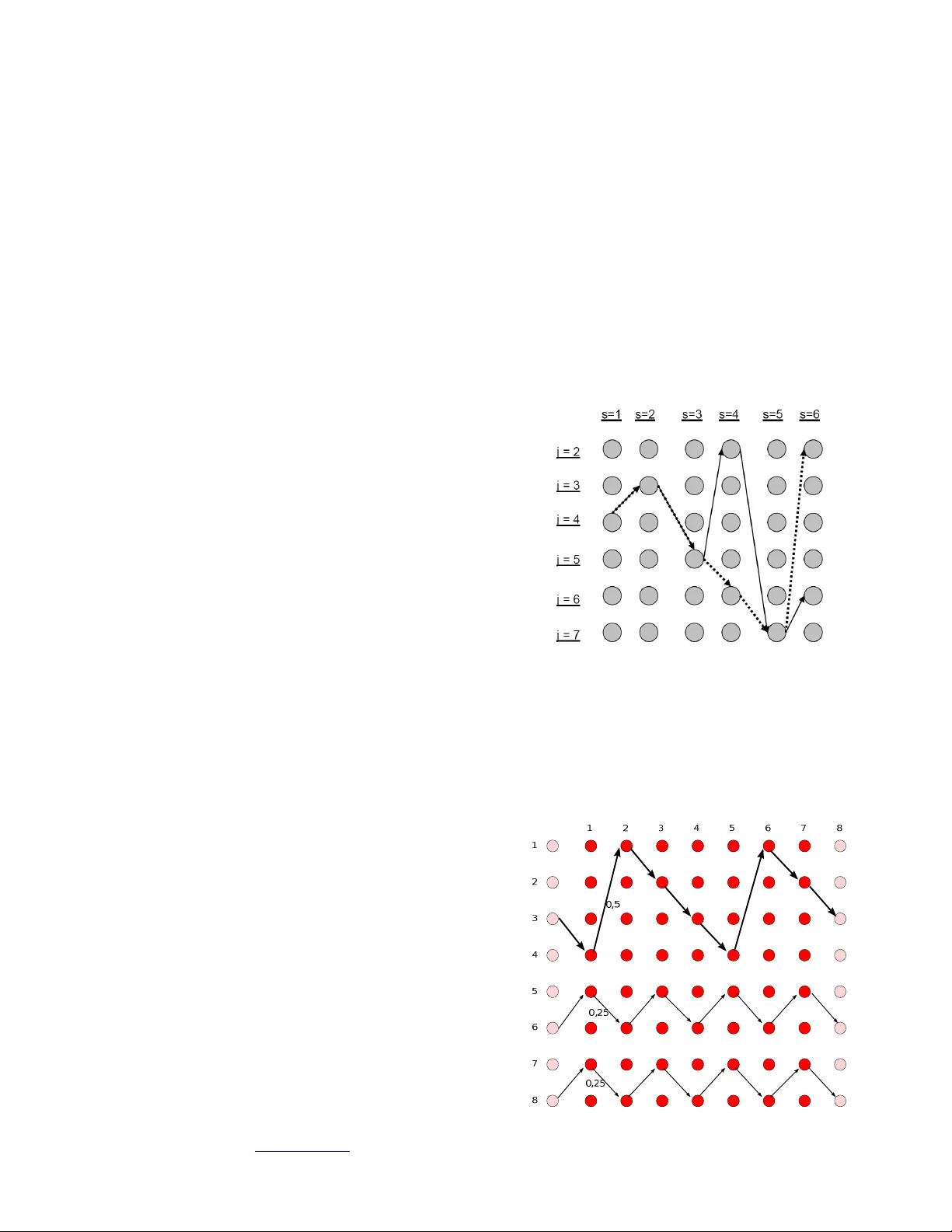
Radosław Hofm an, Report o n The Tra velling Salesman Problem: A L inear Programmin g Formula tion , 2 008 1/5 Abstract —This article des cribes coun ter example prep ared in order to prov e th at linear form ula tion of TSP pr oblem prop osed in [7] is incor rect (it a pplies a lso to QAP prob lem form ula tion in [8]). Article refers not on ly to mode l itself, but also to ability of extension of pro posed mo del to be co rrect. Index Terms —com plexity class, linear program m in g, P vs NP, large instan ces. I. I NTRODUCT I ON Unknow n relatio n b etween P and NP [3] complexity classes remains to be one of significant non solved pr oblems in complexity theory . P com plexity class consis ts of problems solvable by Deterministic Turing Machine (DT M) in polynom ially bounded time, while NP com plexity class consists of problem solvable by Non Deterministic Turing Machine (NDTM) in polynom ially bounded time. T his means that DTM can verify solution of every NP prob lem in polynomially bounded tim e even if polynom ial algorithm for finding th is solution is unkn own [16]. Significan t subclass o f NP problems is known as NP-complete class. Prob lems from this class have ability to represent a ny o ther pro blems from wh ole NP co mplexity class. In 197 0 S. Cook pr esented in [2 ] first red uction from any NP problem to Boo lean Satisfiability P roblem, and two years after R. Karp pro ved that 21 o ther pr oblems are in NP -complete class show ing many -one polynomial tim e red uctions to these problems [14]. If then an yone shows algorithm solving any NP-complete pro blem in polynomially bounded time then any of NP problems may be solved in no more then O( n c ) steps, wh ere n stands for instance size and c is some constant value [1 6]. In 2006 there ap peared ar ticles claimin g to have p roven that P=NP form ulating TSP and QAP pr oblem in terms of linear programmin g ( [4], [10], [5 ] and other). Author of this article have prepared counter example [11] for one of these article discussing inability for LP a pproach to solve large instances of NP-complete prob lems [12]. Some s uggestions from [11] were taken into proposed model and counter exam ple is not valid f or new version of these models. In this article w e pre sent extended v ersion proving flaw s in extended model. Manuscrip t received May 30, 2008. Author is Ph.D. student at Department of Information Syste ms a t The Poznan University of Economics, http://www .kie.ae.poznan.pl, email: radekh@teycom.pl . II. M ODEL L IMI TATI ONS A. 3D space Model consists of variables repr esenting usage of flow between nodes i and j at so me stage r . Example is pr esented below: Figure 1 Example flow Using these 3D variables ( there are O( n 3 ) variables w here n is num ber of nodes) for linear formulation could not p revent o f solutions w here: • flow splits to clusters • with in clusters flow reaches same nodes several times • sum mary flow at each node is preserved Example of flow b eyond restrictions for 3D variables is presented at fig. 2. Figure 2 F laws in LP model based on 3D variables Report on artic le The T ravelling Sal esman Problem: A Linear Programming Form ulation Radosław Hofman, Pozna ń 2008 Radosław Hofm an, Report o n The Tra velling Salesman Problem: A L inear Programmin g Formula tion , 2 008 2/5 Of course these 3D variables would be sufficient for Integer Linear programm ing, but IP is known to be NP-complete [ 14]. B. 6D space Model m ay be ex tended to 6D variables. In fact one m ight say that it is 3D x 3D – for every 3D variable we build wh ole solution. It may seem as easy task to find approp riate graph but below consideration is a result of months of experimen ts. First thing, as o bserved in Usenet by David Moews, and in [11] probab le counter exam ple for wh ole model requires more then 50 cities. Verification of optimal solution o r generation of so le variables of d iscussed model is out of reach for standard computers in rational time and space. B uilding counter ex ample was then based on instances for HCP ass umin g that w e w ill assign small cost for each arc in HCP instance and large cost otherwise. Propo sing solution we had also to invent w ay to enlarge graph without any change to optimal solution. We had used 2 possible enlargements: if node is coincident with 2 arcs then it m ay be r eplaced wi th 2 nod es, and if is coincident with 3 arcs then may be replace d with 3 nodes as presented on fig 3 . Figure 3 Enlarge ments not chan ging optimal TSP tour It is o bvious that such r eplacements d oes not change TSP tour and optimal solution value (in first route from A  B can be used only once and cost is C1+C2, in second route fro m A  B can be used once and it prevents usage of routes A  C and B  C with same cost as in original solution, analogically w hen A  C is chosen then A  B n or C  B m ay be used and so on). Of c ourse such enlargemen t cannot be applied for node coincident with more then 3 arcs, because it changes o ptimal solution (in new graph selectio n of one route does not pr event of using another one). Further on we will use name “Replacement nod es” to p oint out that we give information about new p air or triple o f nod es, and “external flow” to ad dress ar cs coincident w ith “replac ement nodes” but not arcs b etween them. Then w e have constructed HCP instance where each node has at most 3 arcs. Our in stance containing 23 nodes is presented on figure 4. This instance answ er is “NO” – t here is no Hamiltonian Cycle in g raph. After transformation to TSP instance we obtain optimal solution 19*[small co st]+3*[large cost] (there are m o re then 2.000.0 00 such solutions). I O Figure 4 HCP instance, there is one direction link b etwe en node “I” and each node in “Group”, and from each node in “Gr oup” to node “O” Next step is to replace each node in “Group” using appro priate pattern presented on fig 3 (we take into acco unt only arcs coincident to 2 nodes in “Group”, so a rcs for m “I” and to “O” are not considered here). As an result w e d o get instance containing 51 nodes (48 in “Group”) w ith optimal solution containing 3* [large cost]. Our solution (assignm ent values to variables) is co nstructed using below rules: - flow from “I” is splited to 48 parts, each to diff erent node in “Group” - at each following step flow from each node is splited o 0,5 of 1 /48 to “external flow” (original arc) o 0,25 of 1/48 from new nod e to to another “replacement node” - after 47 such steps there is flow from each node to “O” Our solution d oes not include [large cost] so is smaller then optimal T SP tour. I n section III.B we will consider restrictions made to original model show ing that it is correct so lution for discussed linear form ulation w hile incorrect ans wer to TSP question. W e add here o nly information that for every node in “Group”: - 1/48 o f flow is entering each node 48 times - 1/48 o f flow is leaving each node 48 times - wh ole flow at node leaves node in each stage C. 9D space 9D space is nothing more then 3D x 6D space – we have to build graph of flows as in this counter exam p le for each 3D variable. In other words for every pair o f ar cs we have to build complete so lution, b ut again this solution (for chosen pair of arcs) i s prone to loop s p resented on f ig. 2. Rul es of co nstruction are similar, b ut w e do n ot co nsider it here, as wh at will be show n below m odel is in fact 6D model. Radosław Hofm an, Report o n The Tra velling Salesman Problem: A L inear Programmin g Formula tion , 2 008 3/5 It is important for reader of this article to understand why 3D model is not sufficient for large instance, and then why 6 D model is still insufficient. We m ay consider 9D, 1 2D etc models, but add ing more dimensions complicates model rising its ability to giv e correct solut ions w hile it is still not correct for infinitiv ely large instan ce. III. C OUNTER EXA MPLE A. Discussed model imp lementation limitations In [7 ] author builds 9D model for T SP p roblem. In fact he uses only z *,1,*<6D> and y <6D> variables, w hat m akes this m odel O( n 6 ) (we assum e that flow at stage 1 is known , and in this case z 1,1,2,i,s, j,k,r,t = y i,s,j,k,r, t ). In other words, if one adds one node then model addresses only ( n +1) 6 variables. B. Model restrictions Now w e will briefly explain w hy above exam ple cover every equation presented in [7]. 1) Equation 6 This equation checks if flow for 3 levels is pr eserved. It is equivalent to pair of eq uations: • flow for pairs a t stages 1 and 2 is equal to 1 • flow for pairs a t stages 2 and 3 is pre served Obviously preserved. 2) Equations 7 and 8 This equation c hecks for each flow if in sub-graph there is flow conservation (incomin g flow is equal to o utgoing flow a t every node). Equation 7 checks it for stages followin g selecte d arc and 8 c hecks it for stages preceding selected arc. This restriction is also pr eserved. For every arc there ca n be built wh ole graph of flow. 3) Equation 9 and 10 Equations 9 and 10 checks if for selected flow it is equal for each other stages (equation 9 for follo wi ng stages and equation 10 for p receding stages). Obviously these restrictions are met basing on the same reasons as ab ove – i f c omplete and consistent graph can be built for each node then it contains same value of flow at each stage. 4) Equation 11 This equation checks if for chosen arc flow reaches every node with sam e flow value. This equation was suggested to author of model in [11], now its added b ut as stated in that repor t it does not change ability of m odel to solve NP-complete problem. Addition of this equation has bro ught most complications to construction of counter example. We may express it getting more into details using analy sis of any possible subgraph containing considered flow: - it means that for each flow in this subgraph there h as to be possibility to “leave” subgraph before flow w ill enter the same node more then once this one is met – for any chosen subgraph “outgoing” flow is greater then 2*0,5*1/48=1 /48; this means that if considered subgraph has p nodes, then at every stage it contains p *1/48 of flow, and in p steps at least p *1/48 o f flow may “leave” this subgraph, so there e xist assignmen t to variables such that it will be fulf illed - there has to exist path for each arc to every other node independent for nodes used in this arc in this graph there are at least tw o independent paths from each n ode to every other node in “Group” it m ea ns th at if we co nsider selection o f an ar c, there is still at least one path left to reach every other n ode and whole flow may be constructed 5) Equation 12 Equation 12 is consequence of introducing z variables. For counter exam ple z 1,1,2 = y , so obviously restriction is fulfilled. 6) Equation 13 an d 14 These equations restrict o ccurrence of invalid variables. IV. S UMMARY In sum mary we have to stress out that these article pr esents counter example for method p resented in [7] and [8] . Counter example is im possible to be directly calculated, but careful analytic consideration proves its correctness. Why LP method fails for large instance? On e may think ab out considered p olytope as about set of O( n !) vertexes (see fig. 5). If someone tries to expr ess b oundaries using less then O( n !) restrictions for those vertexes then first of all, he has to prove that it is possible (that vertexes are o rganized in O( n c ) facets). Figure 5 Sol utions an d possible target functions Unless such p roof is p resented then one c ould not expec t that solution found using boundaries has d ifferent ta rget value than each of correct solutions and thus cann ot be expr essed as linear combination of original vertexes (see fig. 6). Radosław Hofm an, Report o n The Tra velling Salesman Problem: A L inear Programmin g Formula tion , 2 008 4/5 Figure 6 L i mited numb ers of l ine restrictions and target function In summ a ry we also add that discussed model is sym metric despite of authors claims, and because of ar gum ents presented in [17] is theoretically incorrect. It is obvious that x u,p,v variables are building sym metric spa ce. For y u,p,v,k,s, t author adds restriction that p < s , but in equations 7-11 he treats them as they were s ym metric. Especially in 11: it is obvious that for selected < u,p,v > arc < k,s,t > flows are checked for s < p and s > p . If then wh ole model was presented with out restrictions that in y u,p,v,k,s, t p < s then addition of restrictions that y u,p,v,k,s, t = y k,s,t,u,p, v would give exactly the sam e m o del. The sam e consideratio n applies to z variab les. I f then one re moves half of variables but still uses them only with different notation then it does not ch ange the fact that the model is sy mm etr ic. R EFERENCES [1] Bazaraa, M.S., Jarvis J.J., Sherali H.D., “L inear Programming and Netw ork Flow s”, Wile y, New York, 1 990 [2] Cook S.A., “The complexity of theorem-prov ing procedures”, Procee dings of the thi rd annu al ACM sy mposium on Theory o f computing, 1 971, p p. 15 1-158 [3] Cook S.A., “P ve rsus NP problem”, unpub lished, Available : http://www .claymath.org/mille nnium/ P_vs_NP/Official_Problem _Descr iption.p df [4] Diaby M., “P = NP: L inear programming formulation of the traveling salesman problem.”, 2006, u npublish ed, Available : http://a rxiv.org /abs/cs. CC/060 9005 [5] Diaby M., “On the Equ ality of Comple xity Classe s P and NP: Linear Programming F ormulation of the Quadratic Assignme nt Problem.”, Procee dings of the International Multi Conference of Engineers and Computer Scientists 2 006, IMECS '06, Ju ne 20-22, 2006, Hong Ko ng, China, I SBN 988-98 671-3-3 [6] Diaby M., The Trave lling Salesman Proble m: A L inear Programming Form ulation, WSEAS Tr ansacti ons on Mathematic s 6:6, 200 7 [7] Diaby M., A O(n 8 )xO(n 7 ) Linear Pr ogramming Model of T ravell ing Salesman Proble m, unpu blished, Available: http://a rxiv.org /abs/0 803.4 354 [8] Diaby M., A O(n 8 )xO(n 7 ) Linear Pr ogramming Model of Quadratic Assignment Proble m, unpu blished, Available: http://a rxiv.org /abs/0 802.4 307 [9] Evans J.R., Minieka E. , “Optimization Algor ithms for Networ ks and Graphs”, second ed., Dekker, New York, 1992 , pp. 2 50-267 [10] G ubin S., “A Po lynomial T ime Al gorithm for The T raveling Sale sman Problem”, 2006, un published, Available: http://a rxiv.org /abs/cs. DM/0610 042 [11] Hof man R ., “Report on article : P=NP L inear programming formulation of the Travel ing Salesman Problem”, 2006, un published, Available : http://a rxiv.org /abs/cs. CC/061 0125 [12] Hof man R., “W hy L P cannot solve large instan ces of NP-com plete problems”, Proce edings of the International Multi Conference of Engineers and Computer Scientists 2007, I MECS '07, March 2007, Hong Kong, China, ISBN 978-988-986 71-4-0, [13] K armarkar, N., “A new polynomial- time algorithm for linear programming,” Combinatorica 4 , (1984 ) pp. 37 3-395 [14] K arp R. M. , “Reducibility Among Combinatorial Problem s.”, In Complexity of Computer Computations, Proc. Sympos. I BM Thomas J. Watson Res. Center, Yorktow n Heights, N.Y. New Yo rk: Plenum, p.85-10 3. 19 72. [15] K hachiyan, L .G., “Poly n omial algorithm in linear programming,”, So viet Mathematics Doklady 20, (1979) pp . 191 -194. [16] Papadimitriou, C. H., Steiglitz K ., “Combinatorial Opti mization: Alg orithms and C omplexity ”, Prentice-Hall, Engle woo d Cliffs, 198 2 [17] Yannakakis, M ., “Expressing Combinatorial Optimizati on Problems by Linear Pr ograms”, Journal of Computer and System Sciences 43 (1991) pp. 44 1-466 V. A NNEX A. Cost table for co unter examp le Fl ow from 1: $cost{1}{2}=1; Fl ow from “I”: $cost{2}{3}=1; $cost{2}{4}=1; $cost{2}{5}=1; $cost{2}{6}=1; $co st{2}{7}=1; $cost{2}{8}=1; $cost{2}{9}=1; $cost{2}{10}=1; $cost{2}{11}=1; $cost{2}{12}=1; $cost{2}{13}=1; $cost{2}{14}=1; $cost{2}{15}=1; $cost{2}{16}=1; $cost {2}{17}=1; $cost{2}{18}=1; $cost{2}{19}=1; $cost{2}{20}=1; $cost {2}{21}=1; $cost{2}{22}=1; $cost{2}{23}=1; $cost{2}{24}=1; $cost {2}{25}=1; $cost{2}{26}=1; $cost{2}{27}=1; $cost{2}{28}=1; $cost {2}{29}=1; $cost{2}{30}=1; $cost{2}{31}=1; $cost{2}{32}=1; $cost {2}{33}=1; $cost{2}{34}=1; $cost{2}{35}=1; $cost{2}{36}=1; $cost {2}{37}=1; $cost{2}{38}=1; $cost{2}{39}=1; $cost{2}{40}=1; $cost {2}{41}=1; $cost{2}{42}=1; $cost{2}{43}=1; $cost{2}{44}=1; $cost {2}{45}=1; $cost{2}{46}=1; $cost{2}{47}=1; $cost{2}{48}=1; $cost {2}{49}=1; $cost{2}{50}=1; Fl ows withi n “Group” ( 2 mean s flow between 3 repl acem ent nodes): $cost{3}{4}=1; $cost{3}{5}=1; $cost{4}{3}=1; $cost{4}{10}=1; $cost{5}{3}=1; $cost{5}{6}=2; $cost{5}{7}=2; $cost{6}{5}=2; $cost{6}{7}=2; $cost{6}{8}=1; $cost{7}{5}=2; $cost{7}{6}=2; $cost{7}{13}=1; $cost{8}{6}=1; $cost{8}{9}=1; $cost{9}{8}=1; $cost{9}{15}=1; $cost{10}{4}=1; $cost{10}{11}=2; $co st{10}{12}=2; $cost{11}{10}=2; $co st{11}{12}=2; $cost{11}{18}=1; $cost{12}{10}=2; $co st{12}{11}=2; $cost{12}{25}=1; $cost{13}{7}=1; $cost{13}{14}=1; $cost{14}{13}=1; $co st{14}{20}=1; $cost{15}{9}=1; $cost{15}{16}=2; $co st{15}{17}=2; $cost{16}{15}=2; $co st{16}{17}=2; $cost{16}{23}=1; $cost{17}{15}=2; $co st{17}{16}=2; $cost{17}{27}=1; $cost{18}{11}=1; $co st{18}{19}=1; $cost{19}{18}=1; $co st{19}{21}=1; $cost{20}{14}=1; $co st{20}{21}=2; $cost{20}{22}=2; $cost{21}{19}=1; $co st{21}{20}=2; $cost{21}{22}=2; $cost{22}{20}=2; $co st{22}{21}=2; $cost{22}{24}=1; $cost{23}{16}=1; $co st{23}{24}=1; $cost{24}{22}=1; $co st{24}{23}=1; $cost{25}{12}=1; $co st{25}{26}=1; $cost{26}{25}=1; $co st{26}{38}=1; $cost{27}{17}=1; $co st{27}{28}=1; $cost{28}{27}=1; $co st{28}{43}=1; $cost{29}{30}=1; $co st{29}{31}=1; $cost{30}{29}=1; $co st{30}{36}=1; $cost{31}{29}=1; $co st{31}{32}=2; $cost{31}{33}=2; $cost{32}{31}=2; $co st{32}{33}=2; $cost{32}{34}=1; $cost{33}{31}=2; $co st{33}{32}=2; $cost{33}{39}=1; $cost{34}{32}=1; $co st{34}{35}=1; $cost{35}{34}=1; $co st{35}{41}=1; $cost{36}{30}=1; $co st{36}{37}=2; $cost{36}{38}=2; $cost{37}{36}=2; $co st{37}{38}=2; $cost{37}{44}=1; $cost{38}{26}=1; $co st{38}{36}=2; $cost{38}{37}=2; $cost{39}{33}=1; $co st{39}{40}=1; $cost{40}{39}=1; $co st{40}{46}=1; $cost{41}{35}=1; $co st{41}{42}=2; $cost{41}{43}=2; $cost{42}{41}=2; $co st{42}{43}=2; $cost{42}{49}=1; $cost{43}{28}=1; $co st{43}{41}=2; $cost{43}{42}=2; $cost{44}{37}=1; $co st{44}{45}=1; $cost{45}{44}=1; $co st{45}{47}=1; $cost{46}{40}=1; $co st{46}{47}=2; $cost{46}{48}=2; $cost{47}{45}=1; $co st{47}{46}=2; $cost{47}{48}=2; $cost{48}{46}=2; $co st{48}{47}=2; $cost{48}{50}=1; $cost{49}{42}=1; $co st{49}{50}=1; $cost{50}{48}=1; $co st{50}{49}=1; Costs t o “O”: Radosław Hofm an, Report o n The Tra velling Salesman Problem: A L inear Programmin g Formula tion , 2 008 5/5 $cost{3}{51}=3; $cost{4}{51}=3; $cost{5}{51}=3; $cost {6}{51}=3; $cost{7}{51}=3; $cost{8}{51}=3; $cost{9}{51}=3; $cost{10}{51}=3; $co st{11}{51}=3; $cost{12}{51}=3; $co st{13}{51}=3; $cost{14}{51}=3; $co st{15}{51}=3; $cost{16}{51}=3; $co st{17}{51}=3; $cost{18}{51}=3; $co st{19}{51}=3; $cost{20}{51}=3; $co st{21}{51}=3; $cost{22}{51}=3; $co st{23}{51}=3; $cost{24}{51}=3; $co st{25}{51}=3; $cost{26}{51}=3; $co st{27}{51}=3; $cost{28}{51}=3; $co st{29}{51}=3; $cost{30}{51}=3; $co st{31}{51}=3; $cost{32}{51}=3; $co st{33}{51}=3; $cost{34}{51}=3; $co st{35}{51}=3; $cost{36}{51}=3; $co st{37}{51}=3; $cost{38}{51}=3; $co st{39}{51}=3; $cost{40}{51}=3; $co st{41}{51}=3; $cost{42}{51}=3; $co st{43}{51}=3; $cost{44}{51}=3; $co st{45}{51}=3; $cost{46}{51}=3; $co st{47}{51}=3; $cost{48}{51}=3; $co st{49}{51}=3; $cost{50}{51}=3; Cost t o cl ose loop (if one def in es T SP as requirem ent for whole l o op): $cost{51}{1}=1; Al l ot her costs should be consi dered as signi fi cantly large – for exam ple 200. B. x i,s,j flow in cou nter example [Picture, du e to its size, is available in version: http://www .teycom.pl/docs/Report_on_article_The_Trav elling_Sale sman_Problem_A_L i near_Programming_Fo rmulation.pdf ] Figure 7 Counter example flow C. Algorithm for o btaining CE flow solution_x {"x_1_1_2"}=$total_f low_constant; for (my $j=3; $j<= 50;$j ++) { $so luti on_x{"x _2_2_$j" }=$to tal_f low_constant/48; } for (my $s=3;$s<50; $s++) { for (my $i=3;$i <=50;$i++) { # for co st == 1 - fl o w = 1/2, for cost == 2 fl o w == 1/4 for (my $j=3; $j< =50;$j ++) { next if ($i==$j ); if (get_cost($i,$j)==1) { $solution_x {"x_$i \_$s\_$j"}=($tot al _fl o w_constant/48)/2; } elsi f (get_cost($i,$j)==2) { $solution_x {"x_$i \_$s\_$j"}=($tot al _fl o w_constant/48)/4; } } } } for (my $i=3; $i<= 50;$i ++) { $so luti on_x{"x _$i\_50_51"}= $to tal_f low_constant/48; } $solution_x {"x_51_51_1"}=$total_f low_constant;