Adaptive Ridge Selector (ARiS)

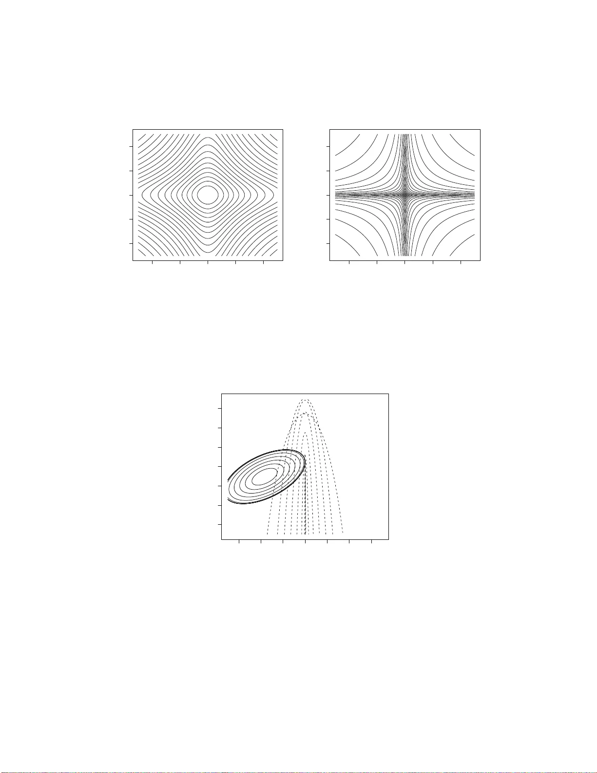
Adaptiv e Ridge Selector (ARiS) No v emb er 2, 2018 Artin Armagan Departmen t of Statistics, Op erations, and Managemen t Science The Univ ersit y of T ennesse e Kno xville, TN, 37996 e-mail: aarmagan@utk.edu and Russell L. Zaretzki Departmen t of Statistics, Op erations, and Managemen t Science The Univ ersit y of T ennesse e Kno xville, TN, 37996 e-mail: rzaretzk@utk.edu Abstract W e in tro d uce a new shrin k age v ariable selection op erator for lin ear m o dels whic h w e term the adap tive ridge sele ctor (ARiS). This approac h is inspir ed b y the r elevanc e ve ctor machine (R VM ), whic h u ses a Ba y esian hierarchical linear setup to do v ariable s electio n and mo del estimation. Extending th e R VM alg o- rithm, w e include a prop er prior d istribution for the precisions of the regression co efficien ts, v − 1 j ∼ f ( v − 1 j | η ), where η is a scalar h yp erparameter. A n o vel fit- ting approac h whic h utilizes the full set of p osterior conditional d istributions is applied to maximize th e j oint p osterior distribution p ( β , σ 2 , v − 1 | y , η ) giv en the v alue of the h y p er-parameter η . An emp irical Ba y es metho d is prop osed for c h o osing η . This appr oac h is con trasted with other regularized least squares 1 estimators including th e lasso, its v ariant s, non n egativ e garrote and ord inary ridge r egression. P erform ance differences are explored for v arious simulated data examples. Results indicate su p erior prediction and m o del selection accu- racy under sp arse setup s and drastic impr o ve men t in accuracy of mo del choic e with in creasing samp le size. KEYW ORDS: Lasso; Elastic net; Shrink age estimation; R VM; R idg e Regr ession; LARS algorithm; Penalize d Least Squares. 1 In tro ducti on Consider the f a miliar linear regression mo del, y = X β + ε where y is an n -dimensional v ector of resp o nses, X is the n × p dimensional mo del matrix and ε is an n -dimensional v ector of indep enden t noise v ariables whic h a r e normally distributed, N p ( 0 , σ 2 I p ) with v ariance σ 2 . Let some ar bitrary subset of t he regression co efficien ts, β , b e zero meaning that the corresp onding regressors do not contribute to the resp onse in the underlying mo del. The ordinary least squares (OLS) estimate is obtained by minimizing t he squared error loss. Although an un biased estimator in this setting, the OLS estimator ma y ha ve large v ariance and will incorrectly estimate the co efficien ts that are zero in the underlying mo del. As a conseque nce, the estimator will usually result in ov erly complex mo dels whic h ma y b e difficult to in terpret. Conv en tionally , an analyst will use subset selection to arrive at a reduced mo del, whic h is easier to in terpret a nd attains b etter prediction accuracy . The subset selection problem has b een studied extensiv ely ( G eorge, 2000) . In cases with larg e n umbers of v ariables, suc h metho ds suffer a fundamental limitation, the need for a greedy algorithm to searc h the discrete mo del space. A more dir ect approa ch to impro ve the prediction accuracy of OLS is based on 2 “shrink age” estimators (Berger, 1985) which trade off increased estimator bias in re- turn for a comp ensating decrease in v aria nce leading to a smaller mean squared error (MSE). A num b er of metho ds hav e b een pro p osed that realize v ariable selection and estimation via some p enalized least squares criteria, e.g. the nonnegativ e garotte (Breiman, 1995), t he la sso (Tibshirani, 199 6), the elastic net (Z ou and Hastie, 2005 ) , the adaptiv e lasso (Zo u, 2006) and more recen tly the D an tzig selector (Candes and T a o , 200 7 ), etc. While traditiona l ridge regression (Ho erl and Kennard, 2000) pro- p oses an ℓ 2 -p enalty o n the co efficien ts, the lasso, and its v arian ts mak e use of the ℓ 1 -p enalty . Tibshirani (199 6 ) demonstrates that the ℓ 1 -p olytop e, unlik e ℓ 2 , can t o uc h the con to urs of the least squares ob jectiv e function on one o r more of the axes leading to estimates of zero for the a sso ciated regression co efficien ts. Tipping (2001) synthe sized sev eral current ideas in the Machine Learning litera- ture and offered tw o imp ortant h ybrid a lgorithms for mo del selection a nd fitting in the k ernel r egression con text. In particular, by com bining kerne l tra nsformations of inde- p enden t v ariables with classical elemen ts of Ba yes ian hierarchical mo deling (Lindley and Smith, 1972) he created the r elev ance v ector mac hine (R VM). This approach is able to efficien tly reduce the h uge feature space created by the k ernel transformations to a v ery parsimonious and predictiv e set impro ving significan tly up on the less sta- tistical suppo r t v ector regression metho d of Druc ker et al. (1 997). This contin uous approac h typ ically conv erges in a finite num b er of steps and pro vides ve ry fast mo del selection for large n um b er o f v ariables without the concerns o f Mon te-Carlo noise or incomplete optimization t ypical of subset selection. A n um b er of extensions to the R VM hav e been offered; see Tipping and Lawrenc e (2005); D’Souza et al. (2 0 04). Recognizing the R VM as a Bay esian random effects mo del, w e offer an alternative form ula t ion whic h offers a more complete hierarc hical structure. One ma jor new de- v elopmen t exploits this hierarchical structure to ra pidly fit the mo del given a fixed 3 v alue for the k ey hyper-para meter. Unlike Tipping (200 1), w e do not in tegra t e the re- gression co efficien ts o ut of the j oin t p osterior distribution o f the parameters. Instead, w e use a conditional maximization pro cedure (Lindley and Smith, 1972) to obtain the p osterior mo de in an elegan t a nd efficien t w ay . Th is a pproac h to mo del fitting w as criticized by (Harville, 19 77, Sec 8.3 ) in the con text o f standar d linear mixed effects mo dels due to the fact tha t it can lead to estimators of v ariance components that are iden tically zero and necessarily far f r om the p osterior mean. Con trary to Harville’s conclusion, w e show that the zeroing effect is theoretically justified a nd can b e easily exploited for v ariable selection. W e refer to this pro cedure a s the adaptive ridge selector (ARiS). Lik e the lasso, this results in a sparse shrink ag e estimator whic h will zero irrelev an t co efficien t s. The marginal likelihoo d p ( y | η ) is maximized ov er the h yp er-par a meter η in order to select the b est estimator. This final empirical Ba ye s step adjusts t he amount of shrink age imp osed on the mo del. Lik e R VM, this alg o- rithm t ypically con v erges in a finite num b er of steps and provides rapid a nd effectiv e mo del selection a nd fitt ing for mo dels with v ery large n um b ers of v ariables. Section 2 in tro duces a hierarc hical random effects mo del similar to tha t of Tipping (2001) and motiv ates our in terest. Section 3 explains ho w the hierarc hical structure is exploited to efficien tly fit the mo del and describes t he steps in the prop osed ARiS algorithm. It also analyzes t he problem in the form of a regula r ized least squares problem and contrasts the estimator with one based on the marginal distribution of the regression co efficien ts. Next, Section 4 fo cuses on deriving the marginal lik eliho o d whic h is used to determine the o ptima l mo del. Because the marginal lik eliho o d is analytically intractable, one must compute it through either analytical or sim ulation based approxim ation. W e provid e a Laplace appro ximation whic h is ev aluated a t the p osterior mo de along with a sim ulation based tec hnique whic h results in somewhat more accurate solutions. Section 5 presen ts comparisons o f the prop osed metho d 4 along with alternativ es on sim ula t ed data examples. Conclusions are discussed in Section 6 . 2 ARiS Beginning with a standard hierarchic al linear mo del (So rensen and Gianola, 2 0 02, Section 6.2.2) w e prop ose a basic mo dificatio n. In this case, the join t p o sterior of the parameters is prop ortional to, p ( β , v − 1 , σ 2 | y , H ) ∝ p ( y | β , σ 2 ) p ( β | σ 2 , v − 1 ) p ( v − 1 | µ, η ) p ( σ 2 ) . (1) Here a normal lik eliho o d is assume d, p ( y | β , σ 2 ) ∼ N ( X β , σ 2 I ), along with a conjugate normal prior on the regression co efficien ts, β , and a t ypical Jeffreys prior on the error v aria nce σ 2 , p ( β | σ 2 , v − 1 ) ∼ N  0 , σ 2 V  (2) p ( σ 2 ) ∝ 1 /σ 2 . (3) As with the relev a nce ve ctor mac hine of Tipping (20 0 1), the v ector v − 1 = diag ( V − 1 ) where V is a diagonal matrix with elemen ts v j , j = 1 , ..., p the recipro cals of whic h are indep endent and iden tically distributed from a g a mma distribution, p ( v − 1 j ) = µ η +1 Γ( η + 1) v − η j exp  − µv − 1 j  (4) where µ is the in verse scale parameter, and η is t he shap e parameter. By definition v j > 0, µ > 0 and η > − 1. Notice that when η = 0, this b ecomes an exp o nen tial distribution whic h we will consider as a sp ecial case. 5 Tipping (2001) sets η = − 1 and µ = 0 whic h leads to a scale inv arian t improp er prior. He then deriv es a marginal lik eliho o d p  y | σ 2 , v − 1 1 , ..., v − 1 p  through direct in- tegration whic h is then maximized with resp ect to σ 2 and v − 1 j . Hypothetically as the algor it hm pro ceeds some v j s will t end tow ard 0 whic h corresp ond to the ir r ele- v ant v ariables in the mo del. Tipping (2001) do es not che c k the v alidity of the join t p osterior densit y havin g assumed an improp er prio r on v − 1 j . In contrast to Tipping (2001), w e choo se not to integrate the regression co efficien ts out of the joint p osterior distribution, but instead pro ceed t o find the mo dal v alue giv en the data and η . Here w e fix µ to b e a v ery small num b er (e.g. mac hine epsilon) and adjust η to con tro l shrink age. Sparsit y is obtained via the combination of these tw o particular priors, p ( β j | σ 2 , v − 1 j ) and p ( v − 1 j ). In tegratio n ov er v − 1 j in the join t prior distribution p ( β j , v − 1 j ) will rev eal that the marginal prior densit y of t he regression co efficien ts is a pro duct of univ ariat e t densities, with a scale of p ( µσ 2 ) / ( η + 1) and degrees o f freedom of 2 η + 2. It is imp ortant to note that the pro duct of univ aria t e t -densities is no t equiv alent to a m ultiv ariate t a nd do es not hav e elliptical contours but instead pro duces ridges alo ng the axes. These ridges can b e made more drastic by c ho o sing the scale parameter to b e small; see Figure 1. Then the p osterior will b e maximized where ev er these ridges first touc h the contours of the likelih o o d. The parameter η plays a ve ry similar role to the regular izat io n para meter of the ridg e regression, lasso, etc., with la r g er v alues encouraging further shrink age. Hence the prop osed hierarc hical structure im- plies indep enden t t priors b eing placed on each regression co efficien t. D ir ect use of suc h t priors w ould obscure the conjugate nature of the mo del. F rom an optimization p ersp ectiv e, a direct use o f suc h priors leads to a non-conv ex ob jectiv e function whic h w ould not b e desirable. As w e will discuss, within the hierarchical structure eac h iteration solv es a simpler con v ex problem leading to an efficien t solution. 6 Once v − 1 j s a r e in t egr a ted o ut of the join t p osterior, the problem can b e seen analogously as a regularized least squares problem a s µ → 0 whic h solv es min β n X i =1 ( y i − x i β ) 2 + λ p X j = 1 log( β 2 j ) . (5) Ha ving sp ecified a complete hierarchic al mo del, the j oin t p osterior distribution of the parameters is obtained b y the pro duct of the lik eliho o d and the sp ecified priors up to a normalizing constan t as p ( β , σ 2 , v − 1 | y , H ) ∝ p ( y | β , σ 2 ) p ( β | σ 2 , v − 1 ) p ( σ 2 ) p ( v − 1 | H ) ∝ ( σ 2 ) − ( n + p 2 +1) p Y j = 1 v − 1 / 2 − η j µ p ( η +1) Γ( η + 1 ) − p × exp  − ( y − X β ) ′ ( y − X β ) + β ′ V − 1 β 2 σ 2  × exp ( − µ p X j = 1 v − 1 j ) (6) where H = ( η , µ ). Theorem 1. Given the priors in (2) , ( 3 ), (4), the p r o duct of these prior densities and the normal likeliho o d, (6) is the ke rnel of a p osterior density function for β , σ 2 , and v − 1 . Pro of f o r this theorem can b e f o und in App endix A. The conditional distributions of the parameters can no w easily b e deriv ed from this join t distribution. i. The regression co efficien ts ar e distributed as multiv ariate normal conditional on the erro r v ariance σ 2 and the prio r cov ariance of the regression co efficien ts V . β | σ 2 , v − 1 , y ∼ N p  e β , e V − 1 σ 2  , (7) 7 where e β = ( X ′ X + V − 1 ) − 1 X ′ y and e V = X ′ X + V − 1 . ii. The error v ar iance is distributed as inv erse gamma conditional up o n all other parameters. p ( σ 2 | β , v − 1 , y ) ∝ ( σ 2 ) − ( n + p 2 +1) × exp  − ( y − X β ) ′ ( y − X β ) + β ′ V − 1 β 2 σ 2  (8) Th us, σ 2 | β , v − 1 , y ∼ inv er se − g amma ( ν ∗ , λ ∗ ) , (9) where ν ∗ = ( n + p ) / 2 and λ ∗ = ( y − X β ) ′ ( y − X β )+ β ′ V − 1 β 2 . iii. The prior precisions of the regression co efficien ts, conditional on all other pa- rameters, follo w a gamma distribution. p ( v − 1 | β , σ 2 , y , H ) ∝ p Y j = 1 ( v − 1 j ) ( 1 2 + η ) exp  − β 2 j + 2 σ 2 µ 2 σ 2 v − 1 i  ∝ p Y j = 1 ( v − 1 j ) ( 3 2 + η − 1) exp  − β 2 j + 2 σ 2 µ 2 σ 2 v − 1 j  . (10) Th us, v − 1 j | β j , σ 2 , y , H ∼ g amma  η ∗ , µ ∗ j  , (11) where η ∗ = 3 / 2 + η and µ ∗ j = ( β 2 j + 2 σ 2 µ ) / 2 σ 2 . Deriving t he full set of conditional distributions has sev eral uses. As is frequen tly done, w e may utilize these to sim ulate from the p osterior distribution using Gibbs sampling. Suc h an approa c h w ould allow us to compute tr aditional Ba ye s estimators for the regression co efficien ts. In Section 3 w e sho w how to use t he conditional 8 distributions to maximize the joint p osterior in a surprisingly simple a nd effectiv e w ay . Maximization will also facilitate computation of the Laplace approximation to the ma r g inal like liho o d ( Tierney and Kadane, 1986). 3 Computing P o sterior Mo des Lindley and Smith (1972) prop osed an optimization algo r it hm to find the j oin t po s- terior mo des; see also Chen et al. (2 001). Once the fully conditional densities of the model parameters are obtained, it is p o ssible t o maximize the joint p osterior distribution b y iterative ly maximizing these conditional densities. Since the conditional p osterior distributions obtained in equations (7), (9), and (11) are well-kno wn distributions with readily av ailable mo des, the Lindley-Smith optimization algorithm b ecomes rather app ealing to implemen t. The mo des for the distributions in equations (7), (9), and (11) resp ective ly are e β =  X ′ X + V − 1  − 1 X ′ y (12) e σ 2 = λ ∗ ν ∗ + 1 (13) e v j = β 2 j + 2 σ 2 µ (1 + 2 η ) σ 2 , j = 1 , 2 , ..., p (14) where ν ∗ , λ ∗ w ere defined in (9). The maximization pro ceeds thro ugh sequen tial re- estimation of e β ( l − 1) , e σ 2( l ) , e v ( l ) j , where l = 1 , ..., m , m is the num b er of iterations, and e β (0) is the OLS estimator. 3.1 Relation to Regularized L S Giv en V , the mo dal v alue of β can b e obtained as a solution to a p enalized least squares problem as with r idg e regression. Since we ha v e a n iterativ e pro cedure, let 9 v ( l ) j b e the j th diag onal o f V ( l ) at the l th iteration and b e giv en. Then the l th it erat e for β is the solution to a similar p enalized least squares problem: β ( l ) = ar g min β n X i =1 ( y i − x i β ) 2 + p X j = 1 β 2 j v ( l ) j . (15) If w e substitute v j with t he estimate from (14) and let µ → 0, w e o bt a in β ( l ) = ar g min β n X i =1 ( y i − x i β ) 2 + ( 1 + 2 η ) p X j = 1 β 2 j ω ( l ) j , (16) where ω ( l ) j = + q β 2( l − 1) j /σ 2( l ) . This pro cedure is essen tially re-w eighting the predictor v aria bles b y the p ositiv e square ro ot of the ratio b etw een the curren t estimate of t he co efficien ts and the residual v ar ia nce due to them. After this re-w eighting pro cedure, the pr o blem takes the form of a standard ridge regression, β ∗ ( l ) = ar g min β ∗ n X i =1  y i − x ∗ ( l − 1) i β ∗  2 + ( 1 + 2 η ) p X j = 1 β ∗ 2 j , (17) where β ∗ j = β j /ω j , x ∗ ( l ) i = x ∗ ( l − 1) i ω ∗ ( l ) and x ∗ (0) i = x i . The solution to the problem ab ov e at iteration l is giv en b y β ∗ ( l ) =  X ′∗ ( l ) X ∗ ( l ) + ( 1 + 2 η ) I  − 1 X ′∗ ( l ) y . (18) Hence the mo de is computed through a sequence of re-w eighted r idg e estimators. The final estimate e β ( m ) then can b e r eco v ered as e β ∗ ( m ) ×  Q m l =1 ω ( l ) 1 , ..., Q m l =1 ω ( l ) p  ′ (this multiplic ation is understo o d compo nen t wise). Note that when η = − 1 / 2 , this pro cedure results in the OLS estimator. W e construct a tw o- dimensional example to illustrate the metho d . Consider 10 the mo del y i = β 1 x i 1 + β i 2 x 2 + N (0 , 1), where β 1 = 0 and β 2 = 3. W e generate 30 observ ations and run ARiS fo r η = 0. Figure 2 clearly demonstrates how the shrink age pro ceeds througho ut our algorithm. The constrained regio n ev entually b ecomes singular along the dimension whic h has no contribution to the resp o nse in the underlying mo del. ARiS iterativ ely up dates t he constrained region and con v erges to a solution. 3.2 The M arginal P osterior Mo de of β via EM An exp ectation-maximization approach ma y b e used to obtain the marginal p osterior mo de of β . Consider the iden tit y p ( β | y ) = p ( β , σ 2 , v − 1 | y ) p ( σ 2 , v − 1 | y , β ) . (19) T a king the logarithm and then ta king t he exp ectations of b oth sides with r esp ect to p  σ 2 , v − 1 | β ( l )  yields log p ( β | y ) = log p ( β , σ 2 , v − 1 | y ) − log p ( σ 2 , v − 1 | y , β ) = Z log p ( β , σ 2 , v − 1 | y ) p  σ 2 , v − 1 | β ( l )  dσ 2 d v − 1 − Z log p ( σ 2 , v − 1 | y , β ) p  σ 2 , v − 1 | β ( l )  dσ 2 d v − 1 , (20) where β ( l ) is the curren t guess o f β (Sorensen and Gianola, 2002 , pg. 446). The EM algorithm in volv es working with the first term of (20 ). The EM pro cedure in our case w ould consist o f the f ollo wing tw o steps: (i) exp ectation of log p ( β , σ 2 , v − 1 | y ) with resp ect to p  σ 2 , v − 1 | β ( l )  , (ii) maximization of the exp ected v alue with resp ect to β . An iterativ e pro cedure results b y replacing the initial guess β ( l ) with the solution of the ma ximization pro cedure β ( l +1) and rep eating (i) and (ii) un til con v ergence. 11 With a slight c hang e in the hierarc hical mo del used, the ab ov e exp ectation will b ecome quite trivial. Unlik e (2), let us not condition the prio r densit y of β on σ 2 . Under suc h a setup, p  σ 2 , v − 1 | y , β ( l )  = p  σ 2 | y , β ( l )  p  v − 1 | y , β ( l )  . Notice t ha t the conditional p osteriors in ( 9) and (11) no w b ecome p ( σ 2 | β , y ) ∝ ( σ 2 ) − ( n 2 +1) exp  − ( y − X β ) ′ ( y − X β ) 2 σ 2  , (21) p ( v − 1 j | β , y , H ) ∝ ( v − 1 j ) ( 3 2 + η − 1) exp  −  β 2 j 2 + µ  v − 1 j  . (22) Giv en the new prior, let us re-write (6) in the log form excluding the terms that do not dep end on β , σ 2 and v − 1 : log p ( β , σ 2 , v − 1 | y , H ) ∝ − ( n/ 2 + 1 ) lo g( σ 2 ) + (1 / 2 + η ) p X j = 1 log v − 1 j − ( y − X β ) ′ ( y − X β ) 2 σ 2 − β ′ V − 1 β 2 − µ p X j = 1 v − 1 j (23) Next we compute E v − 1 | y , β ( l ) E σ 2 | y , β ( l ) log p ( β , σ 2 , v − 1 | y , H ) as µ → 0: − ( n/ 2 + 1) E σ 2 | y , β ( l ) log( σ 2 ) + (1 / 2 + η ) E v − 1 | y , β ( l ) p X j = 1 log v − 1 j ! − ( y − X β ) ′ ( y − X β ) 2 S 2( l ) /n − ( η + 3 2 ) p X j = 1 β 2 j β 2( l ) j , (24) where S 2( l ) =  y − X β ( l )  ′  y − X β ( l )  . Ha ving completed the exp ectation step, the maximization of ( 24) with resp ect to β yields an estimator as the solutio n to the follow ing sequence of con vex minimization 12 problems: β ( l +1) = ar g min β ( y − X β ) ′ ( y − X β ) + (2 η + 3) p X j = 1 β 2 j nβ 2( l ) j /S 2( l ) (25) Hence, the marginal p osterior mo de of β is extremely similar in form to the join t p osterior mo de. Note that we can still a dopt the we igh ting p erspectiv e men tioned earlier. Recall from Section 2 that the in tegra t io n o v er v − 1 j in the prior distribution o f β j results in a univ ar ia te t -densit y with degrees of freedom 2 η + 2. Therefore, a v a lue of η = − 3 / 2 will actually lead to a flat prior ov er β j resulting in the OLS estimator (note that when η = − 3 / 2, t he k ernel of the t densit y has p ow er 0 resulting in a flat densit y). Also, the solution to the marginal when η = − 1 will b e iden tical to the maximization of the joint p osterior when η = 0. Harville (1977) men tions that the estimator o f Lindley and Smith (1972) based on j oin t maximization may b e far fr om the Ba yes estimator and suggests that the maximization of the margina l mo de of the v ariance comp onents would b e a sup erior approac h. Ab ov e we ha v e sho wn tha t in our case the mo de of the marginal densit y ha s the same f o rm as the joint mo de justifying the conditional maximization approac h. In fact, Tipping ado pt s t he a pproac h suggested b y Harville, maximizing the joint p osterior mo de of v − 1 and σ 2 after in tegrating o ver β but still achiev es the zeroing effect. W e needed a slight c hange in the mo del to ease our w ork for the exp ectation step ab ov e, that is, we made the prior distribution of the regression co efficien ts indep en- den t o f t he error v ar ia nce. One may think that while w e we re trying to show the equiv alence of these t w o solutions (the join t and the marginal solutions), w e actually created tw o differen t mo dels and show that their solutions are identical in form, y et, they do not follo w the same mo del. In the traditio nal Ba yes ian analysis of the linear 13 regression mo dels, the regression co efficien ts are conditioned o v er the noise v ariance. This pro vides an estimator for the regression co efficien ts tha t is indep enden t of the noise v ariance. W e follow ed this con v en tion when w e w ere forming our hierarchic al mo del. How ev er, in o ur case, there is no suc h thing as indep endence b etw een the solutions of the regression co efficien ts a nd the noise v ariance. Although in an explicit statemen t suc h as ( 1 2) it ma y seem that the solution for the r egr ession co efficien ts do es not dep end on the error v ariance, there exists an implicit dep endence through the solution of v − 1 j s. W e could ha ve v ery w ell constructed our hierarc hical mo del using a prio r on regression co efficien ts indep enden t of the noise v ariance. This w o uld lead to a solution that is only slightly differen t. The re-estimation equation in (12), (13) and (1 4) would b ecome e β =  X ′ X + σ 2 V − 1  − 1 X ′ y (26) e σ 2 = ( y − X β ) ′ ( y − X β ) n + 2 (27) e v j = β 2 j + 2 µ 1 + 2 η , j = 1 , 2 , ..., p. (28) No w, the solution for v j is indep enden t o f σ 2 , y et the solution of β explicitly dep ends on σ 2 . That said, the implicit dep endence has b ecome a n explicit one. Th us the iterativ e solution for the regression co efficien ts as µ → 0 can b e written as β ( l +1) = ar g min β ( y − X β ) ′ ( y − X β ) + (2 η + 1) p X j = 1 β 2 j β 2( l ) j /σ 2( l ) (29) in whic h, apart from the tuning quan t ity (2 η + 1) , the only difference with (25) is the plug-in estimator used for the noise v ariance. Ha ving sho wn tha t these pro cedures a r e fundamen tally iden tical in form to eac h other, let us discuss another imp ort an t p oin t, the c ho ice of initial v a lues to start the 14 algorithm. Let us consider the solution follow ing (25) with η = − 1: β ( l +1) =       X ′ X +       S 2( l ) /nβ 2( l ) 1 · · · 0 . . . . . . . . . 0 · · · S 2( l ) /nβ 2( l ) p             − 1 X ′ y (30) W e cannot just plug a n y β (0) as an initial estimator. Consider β (0) = 0 . In this case all the regression co efficien ts will b e zero ed. Or let only a subset of β (0) b e zero. Then in the solution those compo nen ts will remain zero. Although w e are solving a series of simple conv ex problems, the dep endency o f the solution to the initial v alue prov es that here w e are dealing with a multi-moda l ob jectiv e function as w ould b e exp ected. Th us using the OLS estimator as a n initia l v alue will tak e us to a lo cal stationar y p oin t whic h is most lik ely under the supp o rt of the data in hand. T o gain further intuition, let us consider an orthogo na l case and let the predictors b e scaled so that they hav e unit 2-norm, i.e. X ′ X = I . In suc h a case the OLS estimator for β w ould hav e a v ariance-co v ariance matrix b σ 2 I where b σ 2 is a plug-in estimator, e.g. the maximum like liho o d estimator or the bias corr ected estimator. T esting the n ull h yp othesis H 0 : β j = 0, a t -statistic can b e computed for a comp o- nen t b β j as b β j / b σ 2 . Notice in (30) the quan tities at the diagonal of t he second piece under the matrix in v erse op eratio n, S 2( l ) /nβ 2( l ) j , resem ble the inv erse of a squared t - statistic. In fact, recall from Section 3.1 that w e for med a sequence of ridge regression problems out of this pro cedure by re-w eighting our predictors b y | β ( l − 1) j /σ ( l ) | whic h is the absolute v a lue of a t -statistic. Thus , follo wing a con ve n tional testing pro cedure, those predictors whic h corresp ond to co efficien ts with larger t -statistics will b e giv en more imp ortance. This is yet another p oint that in tuitiv ely explains our pro cedure. 15 4 Appro ximatin g the marginal lik eliho o d Critical to the ARiS pro cedure is t he c hoice of the hy p er-parameter η . W e prop ose an empirical Bay es estimation of η through the maximization of the marginal lik eliho o d p ( y | η ). Hence, w e m ust in tegrat e the joint p osterior o ve r all parameters, p ( y | η ) = Z θ p ( y , θ | η ) d θ , (31) where θ = ( β , σ 2 , v − 1 ) ′ . In the case of the hierarchic al mo del deve lop ed in Section 2, the direct calculation is in tractable. Below we pro p ose b oth analytical and sim ulation- based appro ximations. 4.1 Laplace app ro ximation A standard ana lytical approxim ation of the mar g inal like liho o d can b e computed using the Laplacian metho d (Tierney and Kadane, 198 6). The approximation is obtained as log ( p ( y | η )) ≈ log h p  y , e θ | η i + p 2 log(2 π ) − 1 2 log   H e θ   , (32) where e θ is the mo de of the joint p osterior and H e θ is the Hessian matrix giv en in B ev aluated at the p osterior mo de. Recall that the ARiS is designed to driv e the v alues of β j and v j to zero for those indep enden t v ariables x j whic h pro vide no explanatory v alue. As µ → 0, the prio r precisions a nd the regression co efficien ts related to irrelev ant indep enden t v ar ia bles will tend tow ard ∞ and 0 resp ectiv ely . In fact w e can see in (40) that alo ng these β j the curv ature appro ac hes ∞ as w e con ve rge to the solution thus driving their v ariance to 0. A t the jo in t p osterior mo de, the corresp onding dimensions of X do not con t r ibute 16 and b ecome irr elev an t. Under the suppo rt of the data, w e claim these v ariables to b e insignifican t and suggest their remo v al from the mo del. The inte gration follows remo v al of these irr elev an t v ariables fr om the mo del. The resulting La pla ce approximation to the log-margina l lik eliho o d is log p ( y | η ) ≈ log p ( e β † , e σ 2 , e v † , y | H ) + p † 2 log(2 π ) − 1 2 log    H e β † , e σ 2 , e v †    . (33) where ( . ) † represen ts the reduced mo del af ter the remo v al of the irrelev an t v a riables at the mo de. 4.2 Numerical in tegration Laplace approximation ma y not p erform w ell in certain cases as will b e seen in Section 5. β and σ 2 can b e analytically integrated out of the join t p osterior g iv en in Eq. 6. The resulting likelih o o d conditioned on the prior v ariances is, p ( y | v − 1 ) ∝   X ′ X + V − 1   − 1 / 2 | V | − 1 / 2  λ + S 2  − ( n + ν ) / 2 , (34) where S 2 = y ′ y − y ′ X  X ′ X + V − 1  − 1 X ′ y ; (35) see also (Chipman et al., 2001, Equations 3.11,3 .1 2). The marg ina l lik eliho o d con- ditioned o v er η can no w b e obtained t hr o ugh integration a s p ( y | η ) = E v − 1 | η [ p ( y | v ) ] where the exp ectation is take n o ve r the prior distribution of v − 1 . In order to ensure efficie n t sampling, w e define a hy p ercub e around the mo de of the join t p osterior in order to obtain a sampling region o ver Q j v − 1 j . The sampling region is the set n v − 1 j | max (0 , e v j − 1 − k σ v − 1 j ) < v − 1 j < e v j − 1 + k σ v i o where e v j − 1 is the mo dal v alue of v − 1 j , σ v − 1 j is the square ro ot of in v erse curv ature at the mo de and k is 17 to b e chose n to adjust the width of the b o x. 5 Examples This section rep orts the results of a sim ulatio n study comparing the ARiS estimates with a n um b er of computationally efficien t p enalized least squares metho ds. In the study w e consider a mo del of the form y = X β + N (0 , σ 2 ). F or eac h data set, w e cen ter y and scale the columns of X so that they hav e unit 2-nor m. The lasso and elastic net were fit using t he lars and elasticnet libraries in R . Mo de l 0 : This mo del is adopted from Zou (2006 ) and is a sp ecial case where the lasso estimate f a ils to impro ve asymptotically . The true regression co efficien ts are β = (5 . 6 , 5 . 6 , 5 . 6 , 0). The predictors x i ( i = 1 , ..., n ) are iid N ( 0 , C ) where C is defined in Zou (2006) (Corollary 1, pg. 1420) with ρ 1 = − . 39 and ρ 2 = . 2 3. Under this scenario, C do es not allow consisten t lasso selection. In this con text Zo u (2006) pr o p oses the adaptiv e lasso (adalasso) f o r consisten t mo del selection. In this setting, w e sim ulate 10 00 data sets from the a b o ve mo del for different comb inations of sample size and error v aria nce. T able 1 rep orts the prop ortion of the cases where the solution paths included t he true mo del f or ARiS, lasso and adaptiv e la sso. W e also rep o rt the results of ARiS in the sp ecial case when η = 0. The results indicate that the ARiS algorithm p erforms nearly as w ell as the ada ptiv e la sso and far b etter than the o r dina r y lasso in t erms of consisten t mo del selection under this particular setting. F or η = 0, the ARiS pro duces a consisten t estimate and do es not require a searc h o v er the solution path. F or medium a nd large v alues of n w e can see that it significan tly outp erforms the lasso. Results fo r the lasso and adalasso ag ree with those o f Zou (2006). W e next compare prediction accuracy and mo del selection consistency using the 18 follo wing t hree mo dels which are dra wn fr om Tibshirani (1996 ). Mo de l 1 : In this example, we let β = (3 , 1 . 5 , 0 , 0 , 2 , 0 , 0 , 0) ′ with iid normal pre- dictors x i ( i = 1 , ..., n ). The pair wise correlation b et wee n the predictors x j and x k are adjusted to b e ( . 5) | j − k | . Mo de l 2 : W e use the same setup as mo del 1 with β j = 0 . 85 for all j . Mo de l 3 : W e use the same setup as mo del 1 with β = (5 , 0 , 0 , 0 , 0 , 0 , 0 , 0) ′ . W e test mo dels 1,2, a nd 3 for tw o differen t sample sizes, n = 2 0 , 100 and t w o noise lev els σ = 3 , 6. This exp erimen t is conducted 100 times under eac h setting. In T able 4, w e rep ort the median prediction error (MSE) on a t est set of 10,000 observ ation for eac h o f t he 100 cases. The v alues in the paren theses give the b o otstrap standard error of the median MSE v alues obtained. C, I and CM resp ectiv ely stand for the n umber of correct predictors chos en, num b er of incorrect predictors c hosen and the pro p ortion of cases (out of 10 0) where the correct mo del was f o und b y the metho d. The b o otstrap standard erro r w as calculated by generating 5 0 0 b o otstrap samples from 1 0 0 MSE v alues, finding the median MSE for eac h case, and then calculating the standard error of t he median MSE. Lasso, adalasso, elastic net, nonnegative garrote, ridg e and ordinary least squares estimates are computed along with t he ARiS estimate. F or the ridge estimator, t he ridge para meter is determined b y a GCV (generalized cross- v alidat io n) t yp e statistic, while f or all the others w e use 10-fold cross-v alidation f or the c hoice of the tuning par ameters. W e also consider the lasso where the t uning parameter is c hosen b y the metho d of Y uan and Lin (2005 ) . ARiS h yp er-parameter η is determined b o th b y the Lapla ce appro ximatio n and the n umerical in tegration to the marginal lik eliho o d. W e also rep o rt the results for the particular case of η = 0. In eac h example the n umerical in tegra tion step of ARiS-eB is carried out for v alues of k = 3 , 10 , 100 , 1000 and only the b est result is rep orted. This is a rather ar bitr a ry c hoice and will depend up on the n um b er of samples dra wn. Mo del 3 is the only 19 example where the same v alue of k is consisten t ly c hosen ( k = 10 00). Mo del 3 demonstrates the most striking feature of the ARiS algo rithm, the ability to iden tify the correct mo del under sparse setups. When utilized along with the empirical Ba yes step, it is a ble t o iden tify the correct mo del in a v ery larg e prop ortion of cases with very lo w prediction error. This is especially surprising for the cases where n = 20 ( σ = 3 , 6). In the case where n = 100 and η = 0 the algorithm still outp erform all other metho ds in terms of correct mo del ch oice and MSE. Among a ll the v ariants of lasso (lasso, adalasso, elastic net, lasso(CML)), la sso(CML) is optimal in terms of prediction accuracy . In the case of n = 1 0 0, it s prediction error is almost iden tical to tha t of ARiS( η = 0) but correct mo del iden tification is strong ly w eak er. Observ e tha t a cross-v alidatio n approac h may not accurately ch o ose the tuning parameter f or the lasso-v aria nts. F or example, a s we mo v ed f rom n = 20 to n = 1 00, the pro p ortion of cases where the correct mo del w as c hosen decreased for all the lasso-v aria n ts except lasso(CML) where the tuning parameter is chosen via an empirical Bay es step similar to our appro a c h. The nonnegative garrote estimator p er- forms quite p o o r ly in this situation along with the ridge and ols estimators. Results indicate that AR iS provides sup erior p erformance for mo del 3. In the case of mo del 1, for n = 100 and σ = 3 , ARiS p erforms b est in terms of prediction accuracy and strongly outp erforms other algorithms in terms of mo del selection accuracy . ARiS( η = 0) o utp erformed other v ersions whic h required a searc h o ver t he solution pat h. Both the Laplace approx imation and the n umerical in tegration fail to detect this v alue of η . F or the case of n = 20, ARiS p erforms within a standard error o f a ll the other estimators in terms of prediction accuracy , y et do es b etter in terms of mo del selection accuracy . The ridge estimator do es almost a s w ell as the lasso-v ar ia n ts in terms of prediction accuracy . Similar results follow f or the case n = 1 00, σ = 6. Ho w ev er, elastic net seems to hav e slightly lo wer prediction erro r . 20 The case n = 20 , σ = 6 sho ws fa irly weak results across all estimators. Mo del 2 demonstrates the biggest w eakness of the ARiS and sev era l other esti- mators. When there are man y small effects presen t in the underlying mo del, these estimators do not p erfo rm we ll since they fa v or parsimony . F or all cases the clear winner is the ridge estimator. 6 Conclus ion W e ha v e introduced a Bay esian mo del fitting and v aria ble selection metho d, ARiS, whic h mak es use of a hierarchic al mo del and enforces parsimon y . The metho d com- bines an efficien t optimization pro cedure whic h is tailo r ed to the fully conditional p osterior densities with v arious tec hniques to deriv e and maximize the marg inal like - liho o d. This dev elopmen t , although radically differen t in detail, is similar in spirit to mo dern implemen tation of the lasso which has b een desc rib ed as a Bay esian pro- cedure whic h combine s a normal lik eliho o d with a L a place prior on the regression co efficien ts; see Tibshirani (19 9 6). Considering the sim ula tion results of Section 5, we note tw o key features of the ARiS: (i) its sup erior prediction and mo del selection a ccuracy when the underlying mo del is sparse, and ( ii) the significant impro v emen t in p erformance accompan ying an increase in the sample size indicating asymptotic consistency . Computationally , for a specific η v alue, ARiS requires one matrix inv ersion at each iteration. This p oin t is ob vious from the description o f the metho d as a series o f ridge regressions. Thu s the computational cost fo r each it era t ion of ARiS is at most O ( p 3 ). In practice, b ecause v ariables are eliminated throughout the pro cedure, the cost often decreases dramatically with eac h iteratio n. Our experiments indicate fast conv ergence of this pro cedure across sample sizes. Lasso metho ds off er a computatio na l adv an tag e 21 due to the lars algo r it hm (Efron et al., 2004) whic h can compute the en tire solution path o f the lasso with the cost o f a single OLS estimator. How eve r, our exp erimen t a l results indicate that t hese metho ds are often inferior in terms of mo del selection and prediction accuracy . Large scale exp erimen ts ha v e show n that the pro cedure remains computationally feasible in situations where the num b er of predictor v ariables is v ery la r g e. Hence the prop osed metho d offers the most a dv antage in problems where one is attempting to select a small or mo derate num b er of v ariables fro m a large initial group, a common situation in ma ny mo dern statistical and data mining applications. An o p en issue is the empirical Ba y es step via nume rical integration. Due to the la r g e scale sim ulations throughout our exp erimen ts w e ha v e only drawn 10 00 samples for the integration of v − 1 . Ob viously in practice a muc h larger set of samples could b e dra wn at little additional cost particularly for sparse mo dels. The pro cess will b ecome more stable as we draw larger samples. In such a case, the c hoice of k ma y just b e fixed at a larger v alue, i.e. k = 1000. 22 The authors w ould lik e to express their appreciation to Rob ert Mee and William M. Br ig gs for their suggestions whic h hav e significan tly added to the clarity of the man uscript. A App endix Pr o of of The or em 1. β and σ 2 can tractably be in tegrated out of (6 ). As a result of this integration, t he only remaining terms that a re dep endent up o n v − 1 j are   X ′ X + V − 1   − 1 / 2 | V | − 1 / 2  y ′ y − y ′ X  X ′ X + V − 1  − 1 X ′ y  − n/ 2 p Y j = 1 p ( v − 1 j ) . (36) It will suffice to sho w that (36) is finitely integrable with resp ect to v − 1 j . | X ′ X + V − 1 | − 1 / 2 | V | − 1 / 2 = | X ′ XV + I | − 1 / 2 < | X ′ XV | − 1 / 2 = | X ′ X | − 1 / 2 | V | − 1 / 2 , (37) and y ′ X  X ′ X + V − 1  − 1 X ′ y 6 y ′ X ( X ′ X ) − 1 X ′ y . (38) Eliminating the terms ag a in that are not dep enden t up o n v j , w e reduce (36) to | V | − 1 / 2 p Y j = 1 p ( v − 1 j ) . (39) In tegrating (39) is equiv alent to Q p j = 1 E v − 1 / 2 j . This expectation is take n with respect to (4 ) and is finite f or µ > 0. 23 B App endix Let θ = ( β , σ 2 , v − 1 ) ′ . The negat ive Hessian, H θ , is giv en b y − ∂ 2 ∂ β k ∂ β m log p ( y , θ | η ) =      1 σ 2  P n i =1 x 2 ik + v − 1 k  , k = m 1 σ 2 ( P n i =1 x ik x im ) , k 6 = m (40) − ∂ 2 ( ∂ σ 2 ) 2 log p ( y , θ | η ) = − ν ∗ + 1 σ 4 + 2 λ ∗ σ 6 (41) − ∂ 2 ∂ v − 1 k ∂ v − 1 m log p ( y , θ | η ) =      v 2 k  1 2 + η  , k = m 0 , k 6 = m (42) − ∂ 2 ∂ β k ∂ v − 1 m log p ( y , θ | η ) =      β k σ 2 , k = m 0 , k 6 = m (43) − ∂ 2 ∂ σ 2 ∂ β k log p ( y , θ | η ) = 1 σ 4 " n X i =1 x ik y i − p X j = 1 x ij β j ! − β k v − 1 k # (44) − ∂ 2 ∂ σ 2 ∂ v − 1 k log p ( y , θ | η ) = − β 2 k 2 σ 4 . (45) References Berger, J. O. Statistic al De cisio n The ory and Ba yesi a n Analysis . New Y ork: Springer (1985). Breiman, L. “Better Subset Regression Using the Nonnega t ive Garr o te.” T e chnomet- rics , 37(4 ):373–384 (199 5). Candes, E. and T ao, T. “The Dantzig Selector: Statistical Estimation When p is Muc h Larger Than n.” Th e Annals of Statistics , 35(6):2 313–2351 (20 0 7). 24 Chen, M.-H., Shao, Q.-M., and Ibrahim, J. G. Monte Carlo Metho ds in Bayesian Computation . Springer (2001). Chipman, H., George, E. I., a nd McCullo ch, R. E. “The Practical Implemen tation of Ba yes ia n Mo del Selection.” IMS L e ctur e Notes - Mono gr aph Series , 38 ( 2 001). Druc ker, H., Burges, C. J. C., K aufman, L., Smola, A., and V apnik, V. “Supp ort V ector Regression Mac hines.” In Mozer, M. C., Jordan, M. I., and P etsc he, T. (eds.), A dvanc es in Neur al I nformation Pr o c essing Systems , volume 9, 155. The MIT Press (1997). D’Souza, A., Vija yakum ar, S., and Sc haal, S. “The Ba y esian Ba ckfitting Relev ance V ector Machine.” In I C ML ’04: Pr o c e e dings of the twenty-first international c on- fer enc e on Machin e le arning , 31 (2004). Efron, B., Hastie, T., Johnstone, I., and Tibshirani, R. “Least Angle Regression.” The Annals of Statistics , 32(2):40 7–499 (2004). George, E. I. “The V ariable Selection Problem.” Journal of the A meric an Statistic al Asso c iation , 95 (2000). Harville, D. A. “Maximum Likelihoo d Approac hes to V ariance Comp onen t Estima- tion and to Related Problems.” Journal of the Americ an S tatistic al Asso ciation , 72(358):32 0–338 (1 977). Ho erl, A. E. and Kennard, R. W. “Ridge Regress ion: Biased Estimation for Nonorthogonal Problems.” T e ch n ometrics , 42(1):80– 86 ( 2 000). Lindley , D. V. and Smith, A. F . M. “Bay es Estimates f o r the Linear Mo del.” Journal of the R oyal Statistic al So ciety. Series B (Metho dolo gic al) , 34 (1972). 25 Sorensen, D. and Gianola, D. Likeli h o o d, Bayesi a n, and MCMC Metho ds in Quanti- tative Genetics . New Y or k: Spring er (20 02). Tibshirani, R. “Regression Shrink age and Selection via the La sso.” Journal of the R oyal Statistic al So ciety. Series B (Metho dolo gic al) , 58(1):267– 288 (1996 ). Tierney , L. a nd Kadane, J. B. “Accurate Approx imations for Posterior Momen ts and Marginal Densities.” Journal of the Americ an Statistic al Asso ciation , 81 (393):82– 86 (1 986). Tipping, M. E. “ Spa r se Bay esian Learning and the Relev ance V ector Mac hine.” Journal of Machine L e arning R ese ar ch , 1 (2001 ). Tipping, M. E. a nd Lawrenc e, N. D . “V ariational inference for Studen t- t mo dels: R o- bust Bay esian inte rp olation a nd generalised comp onen t analysis.” Neur o c omputing , 69 (2 005). Y uan, M. and Lin, Y. “Efficien t Empirical Bay es V ariable Selection and Estimation in Linear Mo dels.” Journal o f the A meric an Statistic al Asso ciation , 100(472) :1215– 1225 (20 0 5). Zou, H. “The Adaptiv e Lasso and Its Or a cle Prop erties.” Journal of the A meric an Statistic al Asso ciation , 101:141 8 –1429 (2006). Zou, H. and Hastie, T. “R egularization and v aria ble selection via the elastic net.” Journal Of The R oyal Statistic al So cie ty Series B , 67(2 ):301–320 (200 5). 26 T ables T a ble 1: Results for mo del 0. n = 60 , σ = 9 n = 120 , σ = 5 n = 300 , σ = 3 Lasso 0.499 0.489 0.498 AdaLasso 0.724 0.935 0.996 ARiS 0.671 0.927 1 ARiS ( η = 0) 0.462 0.895 0.944 27 T a ble 2: Results for mo del 1. MSE (S d) C I CM σ = 3 n = 20 ARiS ( η = 0) 14.341 4 (0.4198) 2.23 0. 89 0.15 ARiS − eB Lap 16.322 0 (0.3434) 1.42 0. 10 0.04 ARiS − eB k =10 14.129 4 (0.5490) 2.05 0. 53 0.17 Lasso 13.832 9 (0.4078) 2.69 1. 79 0.08 Lasso ( cml ) 13.734 9 (0.4959) 2.37 1. 07 0.09 AdaLasso 15.02 72 (0.4686) 2.26 1.2 0.13 E las ticN et ( λ 2 = 1) 13.735 3 (0.3343) 2.73 1.89 0.06 nn − Gar r ote 14.093 4 (0.4435) 2.58 2.48 0.02 Ridg e 13.772 7 (0.4166) 3 5 0 O l s 15.456 8 (0.5224) 3 5 0 n = 100 AR iS ( η = 0) 9.3409 (0.066 0) 2.97 0.29 0.75 ARI S − eB Lap 9.4427 (0.072 4) 2.96 0.5 0.64 ARiS − eB k =3 9.3887 (0.043 2) 2.98 0.42 0.67 Lasso 9.6631 (0.063 1) 3 1.96 0.13 Lasso ( cml ) 9.6605 (0.055 5) 2.99 0.9 0.41 AdaLasso 9.7004 (0.093 9) 2.85 1.08 0.31 E las ticN et ( λ 2 = 0 . 1) 9.5607 (0.067 1) 3 2.02 0.14 nn − Gar r ote 9 .4919 (0.09 01) 3 2.14 0.02 Ridg e 9.8615 (0.075 5) 3 5 0 O l s 9.7112 (0.059 6) 3 5 0 σ = 6 n = 20 ARiS ( η = 0) 53.3 474 (1.5041) 1.37 1.07 0.05 ARiS − eB Lap 52.391 8 (1.2303) 0.89 0.48 0.01 ARiS − eB k =1000 50.333 2 (1.3107) 0.87 0.48 0.01 Lasso 48.946 2 (1.1343) 1.73 1.43 0.03 Lasso ( cml ) 48.116 6 (1.1363) 1.57 1.05 0.04 AdaLasso 52.90 84 (0.8642) 1.42 1.26 0.06 E las ticN et ( λ 2 = 100) 46.583 0 (0.9027) 2.01 1.50 0.02 nn − Gar r ote 58.547 2 (1.5686) 2.44 3.68 0 Ridg e 48.451 6 (0.9443) 3 5 0 O l s 60.107 3 (1.5030) 3 5 0 n = 100 AR iS ( η = 0) 38.66 04 (0.3078) 2.45 0.35 0.39 ARI S − eB Lap 40.235 5 (0.6259) 1.92 0.24 0.23 ARiS − eB k =3 38.591 3 (0.2623) 2.53 0.43 0.41 Lasso 38.844 9 (0.1967) 2.93 2.07 0.15 Lasso ( cml ) 38.664 4 (0.3805) 2.67 0.79 0.33 AdaLasso 39.15 48 (0.2348) 2.61 1.25 0.19 E las ticN et ( λ 2 = 100) 38.469 8 (0.1214) 2.96 1.98 0.10 nn − Gar r ote 39.500 5 (0.2327) 2.92 3.77 0 Ridg e 38.952 6 (0.1671) 3 5 0 O l s 39.276 8 (0.2282) 3 5 0 28 T a ble 3: Results for mo del 2. MSE (S d) C I CM σ = 3 n = 20 ARiS ( η = 0) 15.3053 (0.4332 ) 3.4 0 0 ARiS − eB Lap 19.026 1 (0.1610) 1.60 0 0 ARiS − eB k =3 15.273 9 (0.3484) 3.24 0 0 Lasso 14.0350 (0.3963 ) 5.21 0 0.08 Lasso ( cml ) 14.7502 (0.5382 ) 3.61 0 0 AdaLasso 16.4863 (0.5305 ) 3.66 0 0.01 E las ticN et ( λ 2 = 1) 13.076 5 (0.2780) 6.40 0 0.29 nn − Gar r ote 14.5 337 (0.4887) 5.09 0 0 Ridg e 11.7124 (0.2210 ) 8 0 1 O l s 14.2135 (0.3473 ) 8 0 1 n = 100 AR iS ( η = 0) 10.6279 (0.0781 ) 5.73 0 0.01 ARI S − eB Lap 10.600 8 (0.1936) 4.96 0 0.28 ARiS − eB k =3 10.567 3 (0.0920) 5.86 0 0.02 Lasso 9.7986 (0.042 8) 7.83 0 0.84 Lasso ( cml ) 10.3712 (0.0664 ) 7.24 0 0.44 AdaLasso 10.0627 (0.0889 ) 7.18 0 0.53 E las ticN et ( λ 2 = 0 . 1) 9.7212 (0.062 4) 7.87 0 0.87 nn − Gar r ote 10.0 068 (0.0635) 7.38 0 0.49 Ridg e 9.6199 (0.064 9) 8 0 1 O l s 9.7262 (0.059 6) 8 0 1 σ = 6 n = 20 ARiS ( η = 0) 49.7997 (0.7488 ) 2.13 0 0 ARiS − eB Lap 49.309 5 (0.5579) 1.31 0 0 ARiS − eB k =100 47.948 0 (0.7287) 1.38 0 0 Lasso 47.3209 (0.7402 ) 2.7 0 0.01 Lasso ( cml ) 46.5628 (0.5432 ) 1.95 0 0 AdaLasso 48.7509 (0.5405 ) 2.39 0 0 E las ticN et ( λ 2 = 1000) 46.7312 (0.7713 ) 3.19 0 0 nn − Gar r ote 57.1 654 (2.3273) 5.71 0 0.06 Ridg e 45.6485 (0.8320 ) 8 0 1 O l s 60.2328 (2.0051 ) 8 0 1 n = 100 AR iS ( η = 0) 40.8476 (0.1875 ) 3.22 0 0 ARI S − eB Lap 45.350 6 (0.2318) 1.5 0 0 ARiS − eB k =3 40.801 5 (0.1975) 3.46 0 0 Lasso 38.8809 (0.2259 ) 6.45 0 0.18 Lasso ( cml ) 40.8431 (0.3779 ) 3.74 0 0 AdaLasso 40.4044 (0.2428 ) 4.41 0 0.02 E las ticN et ( λ 2 = 0 . 01) 38.680 8 (0.1883) 6.4 0 0.17 nn − Gar r ote 39.0 697 (0.1628) 6.79 0 0.29 Ridg e 38.4051 (0.1647 ) 8 0 1 O l s 38.6823 (0.1705 ) 8 0 1 29 T a ble 4: Results for mo del 3. MSE (S d) C I CM σ = 3 n = 20 ARiS ( η = 0) 11.257 3 (0.3 805) 1 1.09 0.41 ARiS − eB Lap 9.8811 (0.140 1) 1 0.10 0.92 ARiS − eB k =1000 10.064 2 (0.1 829) 1 0.07 0.95 Lasso 11.573 5 (0.3 479) 1 1.62 0.31 Lasso ( cml ) 10.631 2 (0.3 642) 1 1.59 0.34 AdaLasso 11.592 5 (0.4 178) 1 1.29 0.43 E las ticN et ( λ 2 = 0) 11.5735 (0.3479) 1 1.62 0.31 nn − Gar r ote 12.813 9 (0.4 729) 1 3.43 0.01 Ridg e 15.1850 (0.4721) 1 7 0 O l s 15.354 0 (0.3 310) 1 7 0 n = 100 ARiS ( η = 0) 9.2237 (0.040 4) 1 0.36 0.71 ARI S − eB Lap 9.1452 (0.017 2) 1 0.04 0.97 ARiS − eB k =1000 9.1531 (0.017 2) 1 0.05 0.96 Lasso 9.3343 (0.050 3) 1 1.99 0.21 Lasso ( cml ) 9.223 8 (0.0437) 1 1.28 0.40 AdaLasso 9.3025 (0.057 8) 1 1.27 0.31 E las ticN et ( λ 2 = 0) 9.3343 (0.050 3) 1 1.99 0.21 nn − Gar r ote 9.5324 (0.0460) 1 3.35 0.01 Ridg e 9.8868 (0.061 0) 1 7 0 O l s 9.7112 (0.059 6) 1 7 0 σ = 6 n = 20 ARiS ( η = 0) 45.637 8 (0.7 751) 0.89 1.26 0.28 ARiS − eB Lap 40.392 0 (0.7 669) 0.87 0.28 0.76 ARiS − eB k =1000 41.449 0 (0.7 836) 0.86 0.23 0.80 Lasso 45.041 6 (1.0 000) 0.96 1.72 0.23 Lasso ( cml ) 42.203 8 (1.0 688) 0.96 1.61 0.30 AdaLasso 45.102 0 (1.5 670) 0.9 1.64 0.30 E las ticN et ( λ 2 = 0) 45.0416 (1.0000) 0.96 1.72 0.23 nn − Gar r ote 55.487 9 (2.8 182) 0.98 5.15 0 Ridg e 53.4027 (1.1883) 1 7 0 O l s 60.838 5 (2.5 876) 1 7 0 n = 100 ARiS ( η = 0) 36.9999 (0.1633) 1 0.35 0.72 ARI S − eB Lap 36.598 7 (0.1 946) 1 0.06 0.97 ARiS − eB k =1000 36.831 9 (0.1 794) 1 0.04 0.96 Lasso 37.773 6 (0.1 582) 1 1.99 0.24 Lasso ( cml ) 37.028 3 (0.1 826) 1 1.1 0.47 AdaLasso 37.755 5 (0.2 429) 1 1.24 0.50 E las ticN et ( λ 2 = 0 . 01) 37.561 9 (0.163 4) 1 1.75 0.31 nn − Gar r ote 38.547 7 (0.2 468) 1 5.07 0 Ridg e 38.7256 (0.2456) 1 7 0 O l s 38.845 0 (0.1 913) 1 7 0 30 Figure Captions Figure 1. Con tours of the p enalt y imp osed b y the indep enden t (log) t -prior s f o r µ = 1 and µ = 0 . 001. Figure 2. Visualization of the ARiS algo rithm. Here the solid lines sho w the contours of the least squares function and the dashed lines sho w the adapted constraint region for each iterat ion. 31 Figures −4 −2 0 2 4 −4 −2 0 2 4 (a) −4 −2 0 2 4 −4 −2 0 2 4 (b) Figure 1: Contours of t he p enalt y imp osed b y the indep endent (log) t -priors fo r µ = 1 and µ = 0 . 001. β 1 β 2 −0.6 −0.4 −0.2 0.0 0.2 0.4 0.6 2.4 2.6 2.8 3.0 3.2 3.4 3.6 Figure 2: Visualization of the ARiS algorithm. Here the solid lines sho w the contours of the least squares function and the dashed lines sho w the adapted constraint region for each iterat ion. 32