Correlation function of the Schur process with a fixed final partition

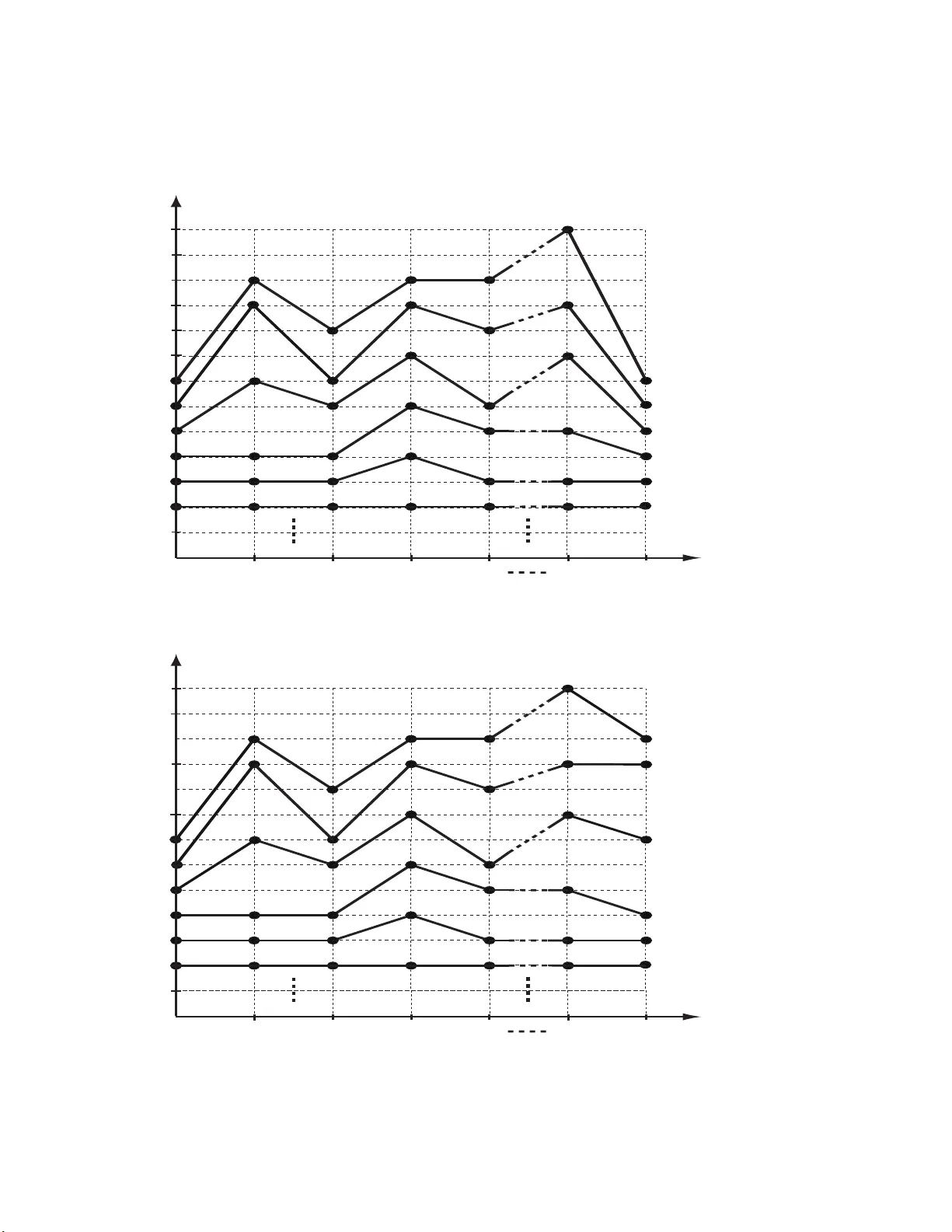
Correlation function of the Sc h ur pro cess with a fixed final partition T. Imamura ∗ and T. Sasam oto † ∗ Institute of Industrial Sc i e nc e, Unive r sity of T okyo, Komab a 4-6-1, Me gur o-ku, T okyo 153-8 5 05, Jap an † Dep artm ent of Mathemat i c s and Inf o r mati c s , Chib a University, Y ayoi-cho 1-33 , Ina g e-ku, Chib a 263-8522, Jap an Abstract W e consider a generalizatio n of the Sc h ur p rocess in whic h a partition evo lve s from the empt y partition in to an arbitrary fixed final partition. W e obtain a double in tegral representa tion of the co rrelation kernel. F or a sp ecial final partition with only one ro w, the edge scaling limit is also d i scussed by the use of the sadd le p oin t analysis. If w e appropriately scale the length of the row, the limiting corr elation k ernel c hanges fr o m the extended Airy k ernel. ∗ e-mail : timamu ra@iis.u-tokyo.ac.jp † e-mail : sasamo to@math.s.chiba-u.ac.jp 1 1 In tro ductio n Recen tly in nonequ ilibrium sto c hastic mo dels wh ich b elong to the one-dimensional Kardar- P arisi-Zhang(KPZ) unive rsality class [1], remark able progress has b een made on the under- standing of the scaling function. The exact f orm of the function is obtained and its relatio n to the random matrix theory is rev ealed [2 , 3, 4, 5, 6]. The common mathematical structure among many o f these mo dels is tha t certain “ cor r elat io n functions” can b e express ed as a determinan t of a correlation kerne l. This structure mak es it p ossible to ex actly analyze the function. The pro cess ha ving the structure is called determinan tal pro cess. The Sc h ur pro cess , whic h w as in tro duced in [7 ], is the ty pical pro cess of the determi- nan tal pro cesses. Let λ b e a par t it ion, i.e. λ = ( λ 1 , λ 2 , · · · ) whe re λ i ∈ { 0 , 1 , 2 , · · · } and λ 1 ≥ λ 2 ≥ · · · . F or a set of partitions { λ (1) , λ (2) , · · · , λ (4 N − 1) } , the measure is defined a s s λ (1) ( a (1) ) 2 N − 1 Y j =1 s λ (2 j − 1 ) /λ (2 j ) ( a (2 j ) ) s λ (2 j +1) /λ (2 j ) ( a (2 j +1) ) ! s λ (4 N − 1) ( a (4 N ) ) , (1.1) where s λ/µ ( a ( i ) ) is the sk e w Sc h ur function of shap e λ/µ in the v ariables a ( i ) = ( a ( i ) 1 , a ( i ) 2 , · · · ). (F or the definition of the Sc h ur function, see (2.10).) Lik e the equation ab o v e, probabilit y measures describ ed b y t he Sch ur function a pp ear in v arious fields in stat istical mec hanics. It has b een know n tha t the Sc h ur function is useful for studying the problems of man y- b ody nonin tersecting random w alk and Bro wnian motion due to its determinan t structure and t he relation to the com binatorics of the Y oung diag ram [8, 9, 10, 11, 12 , 13]. F ur- thermore the w eigh t (1.1) and its v arian t app ear in analyses of v a r ious nonequilibrium pro cess es suc h as the p olyn ucle ar g ro wth(PNG) mo del [14], melting in three-dimensional crystal [15], random tiling pro cess [16], asymmetric exclusion pro cess [17] a nd so on. In order to visualize this mo del, w e explain man y-b ody ra n dom w alk in terpretation of the pro cess intro duc ed in [7]. At t = 0 and t = 4 N , the random walk er lab eled i ( i = 1 , 2 , · · · ) is on the po sition 1 − i on one dimensional lattice Z = {· · · , − 2 , − 1 , 0 , 1 , 2 , · · · } . W e regard λ ( n ) i − i + 1 as the p osition of the i th w alk er, at time n . He re λ ( n ) i is the i th elemen t of the partit io n λ ( n ) = ( λ ( n ) 1 , λ ( n ) 2 , · · · , 0 , 0 , · · · ). On the other hand, the Sc h ur function s λ ( n +1) /λ ( n ) ( a ( n ) ) is interprete d as the transition w eigh t o f the w alk ers from the p osition { λ ( n ) i − i + 1 } i =1 , 2 , ··· at time n to { λ ( n +1) i − i + 1 } i =1 , 2 , ··· at time n + 1. Note that the v a r ia ble s a ( n ) c haracterize the transition w eigh t a t eac h time step. Due to the prop ert y λ ( n ) 1 > λ ( n ) 2 − 1 > · · · > λ ( n ) i − i + 1 > λ ( n ) i +1 − i > · · · , the w alk- ers do not intersec t. Note that the transition we ight (the Sc hu r function) has the Slater determinan t lik e structure ( 2 .10 ). Th us, t his nonin tersecting rando m w alk has the free fermionic feature and w e find that (1 .1 ) describes the (free fermionic) mo del of nonin- tersecting random w alk ers whic h depart from the p ositions (0 , − 1 , − 2 , · · · ) at time 0 and arriv e at the s ame po s itions at time 4 N by w a y of the p os itions { λ ( n ) i − i + 1 } i =1 , 2 , ··· at time n = 1 , 2 , · · · , 4 N − 1 , as depicted in F ig . 1. This type of noninterse cting random w alk is closely related to the PNG mo del. In [14, 18], the authors intro du ced the same t yp e of the random w alk mo del called the m ultilay e r 2 PNG mo del in order to discuss t h e equal-time m ultip oin t correlations of height fluctuations. In this mo del, the p osition of the first w alk er λ ( n ) 1 at time n, ( n = 1 , · · · , 4 N ) repres en ts the height at p osition n and at some fixed time. Not e that in order t o find the dynamics of the first w alk er, we need the informatio n ab out the correlation among the first w alk er and the other w alk ers. Th us, w e fo cus o n the correlation function (see (2.4)) of the Sch ur pro cess in this pap er. W e are also inte rested in s eeing how the initial or final configurat io ns of the w alke rs affect the dynamical b eha vior. In the study of the PNG mo del with an external source [1 9, 20, 21], it has b ee n know n tha t the prop ert y of the heigh t fluctuation c hanges if the exte rnal source is larger than a critical v alue. As w e disc ussed in [21], the external source in the PNG mo del may b e related to the initial or final configurations of the nonin tersecting random w alk mo del. In order to discuss the problem, w e inv estigate the follow ing pro cess in this pap er: s λ (1) ( a (1) ) 2 N − 1 Y j =1 s λ (2 j − 1 ) /λ (2 j ) ( a (2 j ) ) s λ (2 j +1) /λ (2 j ) ( a (2 j +1) ) ! s λ (4 N − 1) /µ (4 N ) ( a (4 N ) ) . (1.2) Here the partitio n µ (4 N ) = ( µ (4 N ) 1 , µ (4 N ) 2 , · · · , µ (4 N ) n , 0 , 0 , · · · ) is arbitrary but fixed. Notice that the weigh t (1.2) is reduced to (1.1) if w e ch o ose µ (4 N ) = φ := (0 , 0 , · · · ). In the in terpretation of nonin tersecting random w alk, the partition µ (4 N ) corresp onds to the final configuration { µ (4 N ) i − i + 1 } i =1 , 2 , ··· . Th us, the w eigh t (1.2) is a nat ura l extension o f the Sc hur pro cess . Fig. 2 illustrat e s the situation. In this pap er, w e obtain the double in tegral for mula of the correlation k ernel of the (dynamical) correlation function (see (2.5)) . F urthermore, b y the use of the form ula, we discuss the asymptotic limit of the correlation function. It will b e shown that if w e appropriately scale the partition µ (4 N ) , t he scaling limit c hanges from case ( 1.1 ). In [7], Okounk o v and Reshetikhin originally deriv ed dete rminant structure of the cor- relation function and the in tegral represen tation of the correlation k ernel in the Sch ur pro cess (1.1) b y the metho d of using t he fermion op erators. T his metho d w as first de- v elop ed in their previous a rticle [22]. In [14], Johansson considered the heigh t fluctuation prop ert y of the (m ultila y er) PNG mo del whic h is esse ntially the same as pro ces s (1.1) and discusse d the deriv ation of the in tegral form ula b y using a prop ert y of a T o eplitz matrix. F urt hermore, the edge scaling limit(see Sec. 2.3) of the correlation kernel is also obtained. A simple linear alg ebraic pro of of the in tegral formula along the approac h in [14] and its Pfaffian analog were discus sed by Boro din and Rains [23]. In the noncolliding Bro wnian motion, whic h w e can regard as the con tinuu m v ersion of F ig.1, the correlation function and its asymptotic f o rm ha v e b een discuss ed in t h e similar situation to Fig . 1 where Bro wnian particles start a nd end at one p oin t. It is found that the pro cess is closely related to the random matrix theory and orthogonal p olynomials [12, 24, 25]. The connection b et w een the dynamics o f the first part icle and P ainlev ´ e equation is also rev ealed [26, 2 7 ]. In case (1.2), on the other hand, the a symptotics of t h e correlation function has not b een discussed y et since an in tegral represen tation of the correlation k ernel has not b een obtained. In this pap er, w e discuss the generalization of the metho d in [14] in order to obtain the in tegral fo rm ula for the correlation ke rnel in pro cess (1.2) a lthough w e could 3 consider the g e neralization of the metho ds in [7, 23]. In the similar situation of noncolliding Bro wnian mot ion where the particles start from one initial p oin t and conv e rge to fixed final p oin ts at the end, it is rev ealed that the pro cess is related to the random matrix mo del with external source and due to the prop erties of m ultiple orthogona l p olynomials , its asymptotic limit can also b e obtained [28, 21]. Recen tly a partial differen tial equation describing the dynamics of the first particle is als o obtained in this situation [29]. How ev er, pro cess (1 .2 ) includes the parameters a ( i ) b y whic h w e can c hange the transition w eigh t ev ery time step. Therefore, ( 1 .2) is a more general pro ces s in the sense t ha t it includes b oth a ( i ) describing the temp orary inhomogeneit y and b oundary par a m eter µ (4 N ) . This pap er is arranged as follo ws. In Sec. 2, w e discuss the background of this study esp ecially the result ab out the pro cess defined by pro ducts of determinant [14] a nd giv e our main results: the do u ble integral form ula of the correlatio n k ernel (Theorem 2.1) and its edge scaling limit (Theorem 2 .2 ). The double in tegral form ula of the correlation k ernel is deriv ed in Sec. 3. In Sec. 4, we discuss the edge scaling limit of the correlation k ernel applying the saddle p oin t method to the in tegral for mula. The Concluding remark is g iv e n in Sec. 5. 2 Correlatio n function 2.1 Determinan t represen tation of correlation function The determinantal s tructure of correlation function ha s b een deriv ed for v arious stochas tic pro cess es suc h as the Sc hur pro cess (1.1) [7] a nd random matrices [30]. F or later discussion, w e consider a class of g eneral measures whic h con tains the ab o v e measures and describ e the result obtained in [14]. This is obtained by g e neralizing the discussion abo u t the random matrix theory in [3 1]. F o r the set { x ( i ) } i =1 , ··· , 4 N − 1 , where x ( i ) = ( x ( i ) 1 , x ( i ) 2 , · · · , x ( i ) M ), w e consider the w eigh t defined b y the pro ducts of determinan ts, w M , 4 N ( { x ( i ) } i =1 , ··· , 4 N − 1 ) = 4 N − 1 Y r =0 det  φ r,r +1 ( x ( r ) i , x ( r +1) j )  M i,j =1 , (2.1) where { φ r,r +1 ( x, y ) } r =1 , ·· · , 4 N are some functions on Z 2 and w e fix x (0) and x (4 N ) suc h that x ( k ) 1 > x ( k ) 2 > · · · > x ( k ) M , k = 0 , 4 N . (2.2) (In [14], some condition is assume d for the f unction φ r,r +1 ( x, y ) suc h that all ob jects that app ear in the discussion con v erge.) By using Lindstr¨ om-Gess el-Viennot’s method [32 , 3 3] (see also [34]), w e find that under condition (2.2), the w eigh ts assigned fo r all configurations but those satisfying x ( i ) 1 > x ( i ) 2 > · · · > x ( i ) M (2.3) 4 v anis h. Namely , when w e interpret x ( j ) i as the p osition of the particle labeled i at time j as in the previous section, the w eigh t do es not v anish only in the case where the particles do not intersec t. The correlation function of the measure (2.1) R ( x (1) 1 , · · · , x (1) k 1 , · · · , x (4 N − 1) 1 , · · · , x (4 N − 1) k 4 N − 1 ) is defined a s R ( x (1) 1 , · · · , x (1) k 1 , · · · , x (4 N − 1) 1 , · · · , x (4 N − 1) k 4 N − 1 ) = 1 Z    4 N − 1 Y i =1 ∞ X x ( i ) k i +1 , ··· ,x ( i ) M = −∞    w M , 4 N ( { x ( i ) } i =1 , ··· , 4 N − 1 ) , (2.4) where Z = Q 4 N − 1 i =1 P ∞ x ( i ) 1 , ··· ,x ( i ) M = −∞ w M , 4 N ( { x ( i ) } i =1 , ··· , 4 N − 1 ) is the normalizatio n constan t. In [14], Joha nsson sho w ed that it can b e represen ted as the determinan t, R ( x (1) 1 , · · · , x (1) k 1 , · · · , x (4 N − 1) 1 , · · · , x (4 N − 1) k 4 N − 1 ) = det  K ( r , x ( r ) j r ; s, x ( s ) j s )  1 ≤ r,s ≤ 4 N − 1 , 0 ≤ j r ≤ k r , 0 ≤ j s ≤ k s . (2.5) The correlation k ernel K ( r 1 , x 1 ; r 2 , x 2 ) is express ed as K ( r 1 , x 1 ; r 2 , x 2 ) = ˜ K ( r 1 , x 1 ; r 2 , x 2 ) − φ r 1 ,r 2 ( x 1 , x 2 ) . (2.6) Here, φ r,s ( x, y ) = ( P ∞ x r +1 = −∞ · · · P ∞ x s − 1 = −∞ φ r,r +1 ( x, x r +1 ) · · · φ s − 1 ,s ( x s − 1 , y ) , for r < s, 0 , for r ≥ s, (2.7) ˜ K ( r 1 , x 1 ; r 2 , x 2 ) = M X i,j =1 φ r 1 , 4 N ( x 1 , x (4 N ) i )( A − 1 ) i,j φ 0 ,r 2 ( x (0) j , x 2 ) , (2.8) A ij = φ 0 , 4 N ( x (0) i , x (4 N ) j ) . (2.9) Hence, w e find t ha t in g e neral class of measures, whic h is describ ed b y pro ducts of dete r- minan t, the correlation function is represen ted as the determinan t. Noticing the Jacobi-T rudi identit y [35], s λ/µ ( a ) = det  h λ i − µ j + j − i ( a )  , (2.10) where h k ( a ) is the k th complete symmetric p olynomial in v ariables a = ( a 1 , a 2 , · · · ), h k ( a ) = X i 1 ≤···≤ i k a i 1 · · · a i k , (2.11) 5 w e easily find that the w eigh t ( 1 .2 ) has t he for m of (2.1), i.e., pro ducts of determinan ts under t he following identific ation: x (0) = (0 , − 1 , − 2 , · · · ) , (2.12) x (4 N ) = ( m 1 , m 2 , · · · , m n , − n, − n − 1 , · · · ) , (2.13) m i = µ (4 N ) i − i + 1 , (2.14) x ( j ) = ( λ ( j ) 1 , λ ( j ) 2 − 1 , λ ( j ) 3 − 2 , · · · ) , for j = 1 , · · · , 4 N − 1 , (2.15) φ r,r +1 ( x ( r ) i , x ( r +1) j ) =    h x ( r +1) i − x ( r ) j ( a ( r +1) ) , fo r r eve n , h x ( r ) i − x ( r +1) j ( a ( r +1) ) , fo r r o dd . (2.16) Note that in (2.10), the rank of the determinan t can b e infinite (infinitely man y w alke rs can mo v e); hence, in this case, M in (2.1) and (2.8) is infinit y . Th us, under this iden tifica- tion (2.12)-(2.16) with M → ∞ , the result (2.5)-(2.9) is applicable to case (1 .2). 2.2 Double int egral form ula One of the purp oses of this pap er is to obtain a do uble integral formula of the correlation k ernel in case (1.2), whic h is useful for the analys is of the scaling lim it as N go es to infinit y . In case of the Sch ur pro cess (1.1), the integral form ula was first obtained in [7 ] by using the fermion op erators. In this pap er, ho w ev er, for considering the case (1.2), w e generalize the approac h in [14] o f calculating the in v erse of the matrix A in (2.8) in case (2.12)–(2.1 6). In the case of the Sch ur pro cess (1.1 ) , i.e., the case µ = φ in (2.14), the matrix A is a T o eplitz matrix and it s in v erse A − 1 can b e estimated by using the Wiener-Hopf factorization [14]. Ho w ev er, in case (1 .2), where µ (4 N ) is general, we cannot apply the metho d b ecause A is not a T o eplitz ma t rix an ymore, whic h is the main difficult y of this problem. In this pap er, we dev elop the metho d of estimating A − 1 in the case of t h e we ight ( 1 .2) and giv e the double in tegral formula for the correlation k ernel. In the following theorem, w e consider the situation a ( i ) = ( a ( i ) 1 , a ( i ) 2 , · · · , a ( i ) p , 0 , 0 , 0 , · · · ) , (2.17) where 0 < a ( i ) j < 1 for i = 1 , · · · , 4 N − 1 a nd j = 1 , · · · , p . W e can easily find that the conditions ab o v e ensures the con v ergence of the partition function Z in (2.4). The theorem is summarized as follows. The pro of is giv en in the next section. Theorem 2.1. In the c ase (2 .1 2 ) – (2.17) and r i = 2 u i ( i = 1 , 2) in (2.6) , ˜ K (2 u 1 , x 1 ; 2 u 2 , x 2 ) 6 and φ 2 u 1 , 2 u 2 ( x 1 , x 2 ) in the c orr elation kernel (2.6) b e c ome ˜ K (2 u 1 , x 1 ; 2 u 2 , x 2 ) = 1 (2 π i ) 2 Z C r 1 dz 1 z 1+ x 1 1 Z C r 2 dz 2 z 1 − x 2 2 p Y m =1 Q u 1 i =1 (1 − a (2 i − 1) m /z 1 ) Q 2 N j = u 2 +1 (1 − a (2 j ) m z 2 ) Q 2 N k = u 1 +1 (1 − a (2 k ) m z 1 ) Q u 2 ℓ =1 (1 − a (2 ℓ − 1) m /z 2 ) × z 1 z 1 − z 2 + 1 s µ (4 N ) ( a ) n X j =1 m j − 1 X ℓ ′ =0 h ℓ ′ ( a ) z m j − ℓ ′ 1 n X b =1 ( − 1) j + b z b − 1 2 s ˜ µ ( j ) /ν ( b ) ( a ) ! , (2.18) φ 2 u 1 , 2 u 2 ( x 1 , x 2 ) = 1 2 π i Z C 1 dz z 1+ x 2 − x 1 p Y k =1 u 2 − 1 Y i = u 1 1 1 − a (2 i +1) k z u 2 Y i = u 1 +1 1 1 − a (2 i ) k /z , (2.19) wher e C r i denotes the c on tour with r adius r i satisfying r 1 > r 2 , h m ( a ) is the m th c omplete symmetric p olynomial (2.11 ) in varia bles a = ( a (1) 1 , a (3) 1 , a (5) 1 , · · · , a (4 N − 1) 1 , a (1) 2 , a (3) 2 , a (5) 2 , · · · , a (4 N − 1) 2 , · · · , a (1) p , a (3) p , a (5) p , · · · , a (4 N − 1) p ) , (2.20) and µ (4 N ) = ( µ (4 N ) 1 , µ (4 N ) 2 , · · · , µ (4 N ) n ) = ( m 1 , m 2 + 1 , · · · , m n + n − 1) , (2.21) ˜ µ ( j ) = ( µ (4 N ) 1 + 1 , · · · , µ (4 N ) j − 1 + 1 , µ (4 N ) j +1 , · · · , µ (4 N ) n ) , (2.22) ν ( b ) = (1 , 1 , · · · , 1 | {z } b − 1 , 0 , · · · , 0 | {z } n − b +1 ) . (2.23) As w as discuss ed in [14, 23], the condition ( 2 .17 ) can b e relaxed suc h that the pro duct Q p m =1 Q u 1 i =1 (1 − a (2 i − 1) m /z 1 ) Q 2 N j = u 2 +1 (1 − a (2 j ) m z 2 ) Q 2 N k = u 1 +1 (1 − a (2 k ) m z 1 ) Q u 2 ℓ =1 (1 − a (2 ℓ − 1) m /z 2 ) con v erges. Note that in case m i = 0(the Sc h ur pro cess ), t h e second term in (2.18) v a nishes and it reduces to t he integral for mula in [7]. 2.3 Edge scaling limit The b enefit of the represen tation (2.1 8 ) is that w e can tak e a n asymptotic limit of the correlation k ernel. In this pap er, w e consider the edge scaling limit of the correlation k ernel in the sp e cial situation x (4 N ) = ( m, − 1 , − 2 , · · · ) , (2.24) a (1) = · · · = a (4 N ) = ( α , 0 , 0 , · · · ) . (2.25) In (2.2 4) with m = 0, the scaling limit of the correlation function w as analyzed in [14] in order to study the height fluctuation of the PNG mo del. W e discuss ho w the scaling b eha vior dep ends on the v alue of m . 7 It has b een kno wn that in the case m = 0, the tr a c e of the first par tic le x ( t ) 1 , t = 0 , · · · , 4 N , b eha v es asymptotically lik e lim N →∞ x ( t ) 1 N = A ( t ) := 2 α 2 1 − α 2 + α 1 − α 2 p 4 t/ N − ( t/ N ) 2 . (2.26) This represen ts a semi-circle cen tered at t = 2 N . W e fo cus our atten tion on the fluctuation of t he w alk ers’ p ositions x i , i = 1 , 2 , · · · , around the ab o v e limiting v alue a t t = 2 N . The scaling limit is called the edge scaling limit. Prec isely , x i and 2 u i in (2.18) and (2.19) a re scaled as follo ws: x i = A (2 u i ) N + D N 1 / 3 ξ i , (2.27) 2 u i = 2 N + 2 C N 2 / 3 τ i , (2.28) where A ( t ) is defined in (2.26) and D = α 1 / 3 1 − α 2 (1 + α ) 4 / 3 , C = (1 + α ) 2 / 3 α 1 / 3 . (2.29) The exp onen t 1 / 3 (resp.2 / 3) in (2.27) (resp. (2.28)) c haracterizes the one-dimensional KPZ univ ersalit y [2, 3, 4, 5, 6]. W e also scale m in (2.24) as m = A (2 N ) N + B N 2 / 3 ω , ( 2 .30) where B = 2 α 2 / 3 (1 − α )(1 + α ) 1 / 3 . (2.31) Our result of t h e scaling limit is summarized as f o llo ws. The pro of will b e give n in Section 4 . Theorem 2.2. In the situation (2.24 ) – (2.31) , the c orr el a t ion kernel has the fol lowing sc aling limit lim N →∞ K (2 u 1 , x 1 ; 2 u 2 , x 2 ) D N 1 / 3 P =        K 2 ( τ 1 , ξ 1 ; τ 2 , ξ 2 ) + R ∞ 0 dλe λ ( τ 1 + ω ) Ai( ξ 1 − λ )Ai( ξ 2 ) , τ 1 + ω ≤ 0 , K 2 ( τ 1 , ξ 1 ; τ 2 , ξ 2 ) − R ∞ 0 dλe − λ ( τ 1 + ω ) Ai( ξ 1 + λ )Ai( ξ 2 ) +Ai( ξ 2 ) exp  − ( τ 1 + ω ) 3 3 + ξ 1 ( τ 1 + ω )  , τ 1 + ω > 0 , (2.32) wher e D is defi ne d in (2.29) , P (se e (4.4) ) is a factor which do es not c ontribute the deter- minant in (2.5) , and K 2 ( τ 1 , ξ 1 ; τ 2 , ξ 2 ) = ( R ∞ 0 dν e − ν ( τ 1 − τ 2 ) Ai( ξ 1 + ν )Ai( ξ 2 + ν ) , τ 1 ≥ τ 2 , − R 0 −∞ dν e − ν ( τ 1 − τ 2 ) Ai( ξ 1 + ν )Ai( ξ 2 + ν ) , τ 1 < τ 2 . (2.33) 8 When m = 0 in (2 .2 4 ), whic h corresp onds to case (1.1)( µ (4 N ) = φ ), only the term K 2 ( τ 1 , ξ 1 ; τ 2 , ξ 2 ) is left since this case corresp onds to ω → −∞ . The correlation k ernel K 2 ( τ 1 , ξ 1 ; τ 2 , ξ 2 ) is called the extended Airy k ernel, whic h app eared in t h e random matrix theory [36, 37, 38, 39] and the PNG mo del [1 4 , 18]. Recen tly , the correlation k ernel (2.3 2) has also app eared in v arious fields suc h as the random matrix with external source (in- cluding the noncolliding Bro wnian motion with pinned initial or final condition) [2 1 , 29], the PNG mo del with an external source [40, 20], statistics [41], and so o n. 3 In tegral repres en tation for the correlatio n k ernel In this section, w e g ive the pro of of Theorem 2.1 . F ir st, w e represen t φ r,r +1 ( x, y ) (2.1 6 ) in terms of the v ertex op erators defined in (A.5). The analysis of the Sc hur pro cess using the v ertex op erators we re dev elop ed in [7, 22]. Ho w ev er, note that in o ur analysis, w e adopt the one-particle basis whereas in [7, 22], infinitely-man y par t icle state is c hosen as a basis. Basic prop erties of the v ertex op erators and symmetric functions are summarized in App end ix A. First, w e prov e (2.19). F rom (2.10) and (A.13), w e ha v e φ r,r +1 ( x, y ) = ( h y | H + ( s ( r +1) ) | x i , for r ev en , h y | H − ( s ( r +1) ) | x i , for r o dd . (3.1) Here, the para meter s ( j ) = ( s ( j ) 1 , s ( j ) 2 , · · · ) is connected to a ( j ) in (1.2) as s ( j ) k = 1 k p X i =1 a ( j ) k i . (3.2) By using (3.1) and (A.9), we can express φ 2 u 1 , 2 u 2 (2.7) as φ 2 u 1 , 2 u 2 ( x 1 , x 2 ) = h x 2 | u 2 − 1 Y i = u 1 H + ( s (2 i +1) ) u 2 Y j = u 1 +1 H − ( s (2 j ) ) | x 1 i . (3.3) By a pp lying (A.6) and (A.7) to this equation, w e easily get (2.19). 9 Next, w e consider the in tegral form of ˜ K . Eq. (2.8) is written as ˜ K (2 u 1 , x 1 ; 2 u 2 , x 2 ) = 1 (2 π i ) 2 Z C r 1 dz 1 z 1+ x 1 1 Z C r 2 dz 2 z 1 − x 2 2 z 1 z 2 ∞ X i,j =1 z x (4 N ) i − 1 1 A − 1 ij z x (0) j +1 2 ∞ X a = −∞ φ 2 u 1 , 4 N ( a, x (4 N ) i ) z a − x (4 N ) i 1 ! × ∞ X b = −∞ φ 0 , 2 u 2 ( x (0) j , b ) z x (0) j − b 2 ! = 1 (2 π i ) 2 Z C r 1 dz 1 z 1+ x 1 1 Z C r 2 dz 2 z 1 − x 2 2 z 1 z 2 ∞ X i,j =1 z x (4 N ) i − 1 1 A − 1 ij z j 2 × 2 N − 1 Y i = u 1 γ ( z − 1 1 , s (2 i +1) ) 2 N Y j = u 1 +1 γ ( z 1 , s (2 j ) ) u 2 − 1 Y k =0 γ ( z − 1 2 , s (2 k +1) ) u 2 Y ℓ =1 γ ( z 2 , s (2 ℓ ) ) . (3.4) Here, γ ( z , s ) is defined in (A.12) and C r i ( i = 1 , 2) denotes the con tour cen tered at the origin anticlockw ise with radius r i satisfying r 2 < r 1 . In the second equalit y , w e use (3.3) and (A.6)–(A.8). Th us, what w e hav e to do is to obtain an explicit f o rm of t he in v erse of the (semi-infinite) matrix A (2 .9 ) in case (2.12)– (2.16) and calculate P ∞ i,j =1 z x (4 N ) i − 1 1 A − 1 ij z j 2 . F rom (3.3), the matrix A in o ur case (2.12)–(2.1 6 ) can b e expressed as A ij = h x j | Λ + ( s )Λ − ( s ′ ) | 1 − i i , (3.5) where x j (= x (4 N ) j ) = ( m j , for 1 ≤ j ≤ n, 1 − j, for n + 1 ≤ j, (3.6) Λ + ( s ) = 2 N Y j =1 H + ( s (2 j − 1) ) , Λ − ( s ′ ) = 2 N Y j =1 H − ( s (2 j ) ) , (3.7) s = ( s (1) , s (3) , · · · , s (4 N − 1) ) , s ′ = ( s (2) , s (4) , · · · , s (4 N ) ) . (3.8) In order to get A − 1 , we introduce the follow ing matrix: A ′ ij = h 1 − j | Λ − 1 − ( s ′ ) P ′ Λ − 1 + ( s ) | x i i , (3.9) where P ′ is a deformed pro j ection op e rator P ′ = ∞ X j =1 | 1 − j ih x j | . (3.10) Note that when n = 0 in (3 .6 ), P ′ b ecome s an o rdin ary pro jection op erator P defined as P = ∞ X j =1 | 1 − j ih 1 − j | . (3.11) 10 By t he use of P ′ and P , w e can express the pro duct A ′ A a s ( A ′ A ) ik = h x k | Λ + ( s )Λ − ( s ′ ) P Λ − 1 − ( s ′ ) P ′ Λ − 1 + ( s ) | x i i . (3.12) Let us fo cus on the term P Λ − 1 − ( s ′ ) P ′ = ∞ X p =1 ∞ X p ′ =1 | 1 − p ih 1 − p | Λ − 1 − ( s ′ ) | 1 − p ′ ih x p ′ | . (3.13) Noticing 1 − p ′ < 0 a n d < j | Λ − 1 − ( s ′ ) | i > = 0 for j > i , whic h immediately follow s from definition (3.7), w e ha v e P Λ − 1 − ( s ′ ) P ′ = Λ − 1 − ( s ′ ) P ′ . (3.14) Namely , we can c hange P in to the iden tity op erator in (3.13). Th us, w e obtain ( A ′ A ) ik = h x k | Λ + ( s ) P ′ Λ − 1 + ( s ) | x i i . (3.15) Note that when n = 0, one can easily find that P ′ (= P ) can a lso b e changed into the iden tit y op erator in (3.15) fro m the similar discussion ab out (3.1 4). Th us, in the case n = 0, A ′ A = 1 or, equiv a lently , A ′ is no thin g but A − 1 . In the case of general n , w e can represen t the matrix A ′ A in t erms of c j − k ( s ) and d j − k ( s ) defined in (A.14) and (A.15) resp ectiv ely , i.e., c j − k ( s ) = h j | Λ + ( s ) | k i = h k | Λ − ( s ) | j i , d j − k ( s ) = h j | Λ − 1 + ( s ) | k i = h k | Λ − 1 − ( s ) | j i . (3.16) By no ting c j − k = d j − k = 0 for j − k < 0, w e get A ′ A =             a 11 a 12 · · · a 1 n a 21 a 22 · · · a 2 n . . . . . . . . . a n 1 a n 2 · · · a nn a n +11 a n +12 · · · a n +1 n 1 . . . . . . . . . 1 . . . . . . . . . . . .             , (3.17) where the region after the n + 1th column is equiv alen t to the unit matrix and a ik = ( P i j =1 d m j − m i ( s ) c m k + j − 1 ( s ) , 1 ≤ i ≤ n, 1 ≤ k ≤ n, P i j = n +1 c m k + j − 1 ( s ) d i − j ( s ) + P n j =1 d m j + i − 1 ( s ) c m k + j − 1 ( s ) , n + 1 ≤ i, 1 ≤ k ≤ n. (3.18) 11 Here, m i is defined in (2.14). No te that the matrix A ′ A is almost the unit matrix. W e easily find that the inv ers e of the matrix A ′ A ha s the following form: B := ( A ′ A ) − 1 = 1 b 0             b 11 b 12 · · · b 1 n b 21 b 22 · · · b 2 n . . . . . . . . . b n 1 b n 2 · · · b nn b n +11 b n +12 · · · b n +1 n b 0 . . . . . . . . . b 0 . . . . . . . . . . . .             . (3.19) By intro duc ing A ′′ := ( a ij ) n i,j =1 , ˜ A ′′ ( j i ) : j i cofactor of A ′′ , (3.20) C = ( c m j + i − 1 ( s )) n i,j =1 , (3.21) w e find that the elemen ts b 0 and b i,j can b e expressed as b 0 = det A ′′ = det C , (3.22) b ij =                                ˜ A ′′ ( j i ) , 1 ≤ i ≤ n, 1 ≤ j ≤ n − det               a 11 a 12 . . . a 1 n . . . . . . . . . a j − 11 a j − 12 . . . a j − 1 n a i 1 a i 2 . . . a in a j +11 a j +12 . . . a j +1 n . . . . . . . . . a n 1 a n 2 . . . a nn               = − P n k =1 a ik b k j , n + 1 ≤ i, 1 ≤ j ≤ n . (3.23) Th us the in v erse of the matrix A (2.9) is represen ted as A − 1 = B A ′ =           1 b 0 P n k =1 b 1 k A ′ k 1 1 b 0 P n k =1 b 1 k A ′ k 2 . . . . . . . . . 1 b 0 P n k =1 b nk A ′ k 1 1 b 0 P n k =1 b nk A ′ k 2 . . . 1 b 0 P n k =1 b n +1 k A ′ k 1 + A ′ n +1 , 1 1 b 0 P n k =1 b n +1 k A ′ k 2 + A ′ n +1 , 2 . . . 1 b 0 P n k =1 b n +2 k A ′ k 1 + A ′ n +2 , 1 1 b 0 P n k =1 b n +2 k A ′ k 2 + A ′ n +2 , 2 . . . . . . . . .           . (3.24) 12 By using this ex pression for A − 1 , w e can r epresen t P ∞ i,j =1 z x (4 N ) i − 1 1 A − 1 ij z j 2 in (3.4) as ∞ X i,j =1 z x i − 1 1 ( A − 1 ) ij z j 2 = ∞ X i = n +1 ∞ X j =1 z − i 1 A ′ ij z j 2 + 1 b 0 n X k =1 ∞ X i = n +1 z − i 1 b ik ∞ X j =1 A ′ k j z j 2 + 1 b 0 n X k =1 n X i =1 z m i − 1 1 b ik ∞ X j =1 A ′ k j z j 2 . (3.25) After quite lengthy calculations of this equation, w e obtain the following expression ∞ X i,j =1 z x i − 1 1 ( A − 1 ) ij z j 2 = ∞ X k =1  z 2 z 1  k + 1 det C n X j =1 m j − 1 X ℓ ′ =0 c ℓ ′ ( s ) z m j − 1 − ℓ ′ 1 n X b =1 z b 2 ˜ C ( bj ) ! × 2 N Y j =1 γ − 1 ( z − 1 1 , s (2 j − 1) ) γ − 1 ( z 2 , s (2 j ) ) , (3.26) where ˜ C ( bj ) is the bj cofactor of matrix C . The pro of o f this equation is giv en in App endix B. By no t ic ing (A.13) and (A.14), w e can rewrite c ℓ ′ ( s ), det C , and ˜ C ( bj ) as c ℓ ′ ( s ) = h ℓ ′ ( a ) , (3.27) det C = s µ (4 N ) ( a ) , (3.28) ˜ C ( bj ) = ( − 1) j + b s ˜ µ ( j ) /ν ( b ) ( a ) , (3.29) where a, µ (4 N ) , ˜ µ ( j ) , and ν ( b ) are defined in (2.20)-(2.23), respective ly . By substituting (3.26)-(3.2 9 ) in to (3.4) a n d noting (3.2) and (A.12), w e get the desired expression (2.18). 4 Asymptotic analysis In this section, w e give the proo f of Theorem 2.2. W e in v estigate the a symptotics of the correlation k ernel b y the use of the saddle p oin t analysis. In case (2.24) a n d (2.25), the correlatio n k ernel defined in (2.1 8 ) and (2.1 9) reduces to K (2 u 1 , x 1 ; 2 u 2 , x 2 ) = ˜ K (2 u 1 , x 1 ; 2 u 2 , x 2 ) − φ 2 u 1 , 2 u 2 ( x 1 , x 2 ) = 1 (2 π i ) 2 Z C r 1 dz 1 z 1+ x 1 1 Z C r 2 dz 2 z 1 − x 2 2 z 1 z 1 − z 2 (1 − α/z 1 ) u 1 (1 − α z 2 ) 2 N − u 2 (1 − αz 1 ) 2 N − u 1 (1 − α/z 2 ) u 2 + 1 2 π i Z C 1 dz z 1+ x 2 − x 1 (1 − αz ) u 1 − u 2 (1 − α /z ) u 1 − u 2 + m X j =1 h m − j ( α 2 N ) h m ( α 2 N ) 1 2 π i Z C 1 dz 1 z 1+ x 1 − j 1 (1 − α /z 1 ) u 1 (1 − α z 1 ) 2 N − u 1 × 1 2 π i Z C 1 dz 2 z 1 − x 2 2 (1 − α z 2 ) 2 N − u 2 (1 − α/z 2 ) u 2 , (4.1 ) 13 where C r denotes the contour enclosing the origin a n ticlock wise with radius r and h j ( α 2 N ) is t he j th complete symmetric p olynomial (2 .1 1) in v a riables α 2 N = ( α , α, · · · , α ) | {z } 2 N . (4.2) In [14 ], it w as show n that the first tw o t e rms of the correlation k ernel ab o v e con v erge to the extended Airy ke rnel in the edge scaling limits (2.27) and (2.2 8 ), lim N →∞ D N 1 / 3 (2 π i ) 2 Z C r 1 dz 1 z 1+ x 1 1 Z C r 2 dz 2 z 1 − x 2 2 z 1 z 1 − z 2 (1 − α/z 1 ) u 1 (1 − αz 2 ) 2 N − u 2 (1 − αz 1 ) 2 N − u 1 (1 − α /z 2 ) u 2 + D N 1 / 3 2 π i Z C 1 dz z 1+ x 2 − x 1 (1 − αz ) u 1 − u 2 (1 − α /z ) u 1 − u 2 = P × K 2 ( τ 1 , ξ 1 ; τ 2 , ξ 2 ) , (4.3) where K 2 ( τ 1 , ξ 1 ; τ 2 , ξ 2 ) is defined in (2.33) and P is a prefactor whic h do e s not contribute a determinant, P = (1 − α ) 2(1+ α ) 2 / 3 N 2 / 3 ( τ 1 − τ 2 ) α 1 / 3 e ( τ 3 1 − τ 3 2 ) / 3+ ξ 2 τ 2 − ξ 1 τ 1 . (4.4) Th us, w e only consider the asymptotics of the last term, m X j =1 h m − j ( α 2 N ) h m ( α 2 N ) ψ 1 ( x 1 − j ) ψ 2 ( x 2 ) , (4.5) where ψ 1 ( x 1 − j ) = 1 2 π i Z C 1 dz 1 z 1+ x 1 − j 1 (1 − α/z 1 ) u 1 (1 − α z 1 ) 2 N − u 1 , (4.6) ψ 2 ( x 2 ) = 1 2 π i Z C 1 dz 2 z 1 − x 2 2 (1 − α z 2 ) 2 N − u 2 (1 − α/z 2 ) u 2 , (4.7) under t he scaling (2.27)–(2.31). W e scale j as j = D N 1 / 3 λ. (4.8) Here, D is defined in (2.29). This scaling makes a dominant contribution to the asymptotic limit of (4.5). First, w e consider the function ψ 1 ( x 1 − j ) . By substituting (2.28) into (4 .6), we hav e ψ 1 ( x 1 − j ) = 1 2 π i Z C 1 dz 1 z 1+ x 1 − j − µN 1 exp( N f β ,µ ( z 1 )) , (4.9) where f β ,µ ( z ) = (1 + β ) log ( z − α ) − (1 − β ) log(1 − αz ) − ( µ + 1 + β ) log z , β = C N − 1 / 3 τ 1 , (4.10) 14 and w e fix µ a s µ = 2 α 1 − α 2 ( α + p 1 − β 2 ) = A (2 u 1 ) , (4.11) where A (2 u 1 ) is defined in (2.26). In (4.10), C is defined in ( 2 .29 ). W e find that due to (4.11) , tw o saddle p oin ts of the f unction f β ,µ ( z ) merge to the double saddle p oin t z c ( β ), z c ( β ) = √ 1 + β + α √ 1 − β √ 1 − β + α √ 1 + β . (4.12) W e also hav e the relations f β ,µ ( z c ( β )) dz = d 2 f β ,µ ( z c ( β )) dz 2 = 0 , d 3 f β ,µ ( z c ( β )) dz 3 = 2 D 3 z 3 c ( β ) . (4.13) Since the main con tribution to the in tegral in (4.9) is giv en around z ∼ z c ( β ), z 1 ma y b e transformed to z 1 = z c ( β )  1 − iw 1 D N 1 / 3  ∼ 1 + τ 1 − iw 1 D N 1 / 3 . (4 .14) Then, w e obtain the relations exp( N f β ,µ ( z 1 )) ∼ exp  N  f β ,µ ( z c ( β )) + f ′′′ β ,µ ( z c ( β )) 6 ( z − z c ( β )) 3  = exp( N f β ,µ ( z c ( β )) ) exp  i 3 w 3 1  , (4.15) 1 z x 1 − j +1 − µN 1 ∼ exp(( ξ 1 − λ )( iw 1 − τ 1 )) . (4.16) In (4.16), w e used ( 2 .27) . By using (4.14)– (4.16), and exp ( N f β ,µ ( z c ( β )) ) ∼ ( 1 − α ) 2(1+ α ) 2 / 3 τ 1 N 2 / 3 α 1 / 3 exp( τ 3 1 / 3) , (4.17) w e get D N 1 / 3 ψ 1 ( x 1 − j ) ∼ (1 − α ) 2(1+ α ) 2 / 3 N 2 / 3 τ 1 α 1 / 3 exp  τ 3 1 / 3 − ξ 1 τ 1 + τ 1 λ  × Ai( ξ 1 − λ ) . (4.18) Similarly ψ 2 ( x 2 ) b ecome s D N 1 / 3 ψ 2 ( x 2 ) ∼ (1 − α ) − 2(1+ α ) 2 / 3 N 2 / 3 τ 2 α 1 / 3 exp  − τ 3 2 / 3 + ξ 2 τ 2  × Ai( ξ 2 ) . (4.19) Here, in the equations ab ov e , w e used the integral represen tation o f the Airy function Ai( x ) = Z ∞ −∞ dλe ixλ + i 3 λ 3 . (4.20) 15 Next, w e also apply the saddle p oin t analysis to h m − j ( α 2 N ) /h m ( α 2 N ) in (4.5) under the scaling (2.30) and (4.8) as N → ∞ . F rom (A.12), (A.19), and (2.30), h m − j ( α 2 N ) is expresse d as h m − j ( α 2 N ) = 1 2 π i Z C 1 e − N g ( z ) dz z − j +1 , (4.21) where the con tour C 1 represen ts the unit circle surrounding the orig in antic lo c kwise, and g ( z ) = 2 log(1 − αz ) +  2 α 1 − α + δ  log z , δ = B ω N 1 / 3 . (4.22) The saddle p oin t w c of g ( z ) is w c = 2 α + (1 − α ) δ 2 α + α (1 − α ) δ . (4.23) When we deform the path of z to z = w c  1 + 1 − α α 1 / 2 N 1 / 2 iw  ∼ 1 + ω D N 1 / 3 + 1 − α α 1 / 2 N 1 / 2 iw , (4.24) w e find exp ( − N g ( z )) ∼ exp( − N g ( w c ) − w 2 ) , 1 z − j +1 ∼ e ω λ . (4.25) Therefore, the asymptotic form of h m − j ( α 2 N ) b ecome s h m − j ( α 2 N ) ∼ N − 1 / 2 2 √ π 1 − α α (1 − α ) − 2 N exp − α 1 / 3 ω 2 N 1 3 (1 + α ) 2 / 3 + ω 3 / 3 + ω λ ! . (4.26) Th us, w e get h m − j ( α 2 N ) h m ( α 2 N ) ∼ exp( λω ) . (4.27) F r o m (4.1 8), (4.1 9), and (4.2 7 ), w e obtain D N 1 / 3 m X j =1 h m − j ( α 2 N ) h m ( α 2 N ) ψ 1 ( x 1 − j ) ψ 2 ( x 2 ) ∼ P × Z ∞ 0 dλe λ ( τ 1 + ω ) Ai( ξ 1 − λ )Ai( ξ 2 ) . (4.28) Here the prefactor P is defined in (4.4). F rom (4.3) and (4.28) a n d noting that P do es no t con tribute to determinant calculation, we finally obtain the desired expres sion. Ho w ev er, it is ob vious t ha t this expression is v a lid only f or t he case τ i + ω < 0( i = 1 , 2) b ecause in the case τ i + ω > 0, the in tegration in (4.28) is div ergen t. 16 In order to get the asymptotic fo rm in the latter case, w e need another expression for (4.5). By using (A.19), we rewrite the term P m j =1 h m − j ( α 2 N ) z − j in (4.5), m X j =1 h m − j ( α 2 N ) z j = z m (1 − α /z ) 2 N − 0 X j = −∞ h m − j ( α 2 N ) z j . (4.29) Th us, w e obtain m X j =1 h m − j ( α 2 N ) h m ( α 2 N ) ψ 1 ( x 1 − j ) ψ 2 ( x 2 ) = 1 h m ( α 2 N ) ϕ ( x 1 ) ψ 2 ( x 2 ) − 0 X j = −∞ h m − j ( α 2 N ) h m ( α 2 N ) ψ 1 ( x 1 − j ) ψ 2 ( x 2 ) , (4.30) where ϕ ( x 1 ) = 1 2 π i Z C 1 dz 1 z 1+ x 1 − m 1 (1 − α /z 1 ) u 1 − 2 N (1 − αz 1 ) u 1 − 2 N , (4.31) and ψ 1 ( x )(resp. ψ 2 ( x )) is defined in (4 .6 ) (resp. (4.7)). W e can easily g et the a s ymptotic f orms of ϕ ( x ) by using the saddle p oin t analysis in a manner similar to the deriv ation of (4.26). The result is ϕ ( x 1 ) ∼ N − 1 / 2 2 π 1 / 2 1 − α α (1 − 2 N ) − 2 N (1 − α ) 2(1+ α ) 2 / 3 τ 1 N 2 / 3 α 1 / 3 exp  − α 1 / 3 ω 2 N 1 / 3 (1 + α ) 2 / 3 − τ 2 1 ω − τ 1 ω 2 + ξ 1 ω  . (4.32) F r o m (4.1 9), (4.2 6), and (4.3 2 ), w e ha v e D N 1 / 3 ϕ ( x 1 ) h m ( α 2 N ) ψ 2 ( x 2 ) ∼ P × e − ( ω + τ 1 ) 3 / 3+ ξ 1 ( ω + τ 1 ) Ai( ξ 2 ) . (4.33) Analogous to the deriv ation of (4.28), w e also ha v e − D N 1 / 3 0 X j = −∞ h m − j ( α 2 N ) h m ( α 2 N ) ψ 1 ( x 1 − j ) ψ 2 ( x 2 ) ∼ − P × Z ∞ 0 dλe − λ ( τ 1 + ω ) Ai( ξ 1 + λ )Ai( ξ 2 ) . (4.34) F r o m these tw o relations, w e g et the desired expression also in the case τ i + ω > 0. 5 Conclus ion In this pap er, w e hav e studied the correlatio n function (2.4) of the pro cess (1.2). This pro cess is the g e neralization of the Sch ur pro cess (1.1) [7] in t he sens e that in the picture of nonin tersecting ra n dom walk, the w alk ers end at fixed sites, as depicted in Fig. 2. A t first, w e hav e obtained the integral represen tation of the correlation k ernel (Theorem 2.1). 17 The result is the generalization of the o n e in t he Sc hu r pro cess obtained in [7 , 14, 2 3]. The deriv a t io n is giv en in Sec. 3. The key tec hnique is the calculation of the inv ers e o f the matrix A (2.9) with semi-infinite rank. This tec hnique can b e regarded as the generalization of the one discussed in [14]. Next, b y using the integral represen tation, w e hav e obtained the edge scaling limit of the correlation k ernel in the special case (2.24 ) and (2.25). The result is summarized as Theorem 2.2 a nd the pro of is give n in Sec. 4 . W e ha v e found that the limiting correlation k ernel is equiv a le nt to the one obtained in other determinan tal pro cess es suc h as the rando m matrix with external source, the PNG mo del, and stat istics. W e list the future problems as follow s. 1. In this pap er, w e hav e discussed the a s ymptotics of the corr elat io n k ernel o nly in the simple case (2.2 4) and (2 .25 ), although the pro cess (1 .2) has many parameters µ (4 N ) and { a ( i ) } i =1 , ··· , 4 N . It w ould be intere sting to in v estigate the limiting b eha vior of the correlation k ernel in a more g e neral situation and ho w it dep ends on these parameters. 2. The correlatio n ke rnel ma y b e closely related to the orthogonal p olynomials. In the Sc h ur process, the correlation kernel (the first term in (2.18)) can b e represen ted in terms of the Meix ner p olynomial in the single time case [42]. On t h e o the r hand, it has been recen tly rev ealed tha t the correlation k ernel corresp onding to the random Hermitian matrix with external source can b e expressed in terms of the multiple orthogonal p olynomials [43]. In the discretized pro cess (1.2), is the correlation k ernel related to any discrete ana lo g o f the multiple ortho g onal p olynomial? 3. In Theorem 2.1, the second term in (2.18), which is due to the partition µ (4 N ) in (1.2), can b e expressed b y using the Sc h ur function. This fact raises our hop e that there exists some dee p connection b et w een the pro ces s ( 1.2 ) and the theory of integrable system and represen tation theory . In particular, it is in teresting to view the problem in p ersp e ctiv e of the Kadom tsev-P etviash vili and T o da Lattice hierarc hies [4 4 , 45]. Recen tly , the relationship b et w een t he sto c hastic pro ces ses suc h as the random turn w alk and soliton theory has b een discussed in [45]. This approach may b e useful for studying this topic. A V ertex o p e rators and symmetric fun ctions Let c † j and c i ( i, j ∈ Z = ( · · · , − 1 , 0 , 1 , · · · )) b e the creation and annihilation op erators that satisfy the fermion antic ommutation relation { c i , c † j } := c i c † j + c † j c i = δ ij , ( A.1 ) { c i , c j } = { c † i , c † j } = 0 . (A.2) One particle stat e | i i is defined as | i i = c † i | Ω i , (A.3) 18 where | Ω i is the v acuum stat e without particle. The mo de o perators c ( z ) , c † ( z ) and the v ertex op erators H ± ( s ), where s = ( s 1 , s 2 , · · · ), are defined as follows: c † ( z ) = ∞ X i = −∞ z i c † i , c ( z ) = ∞ X i = −∞ z − i c i , (A.4) H ± ( s ) = exp ∞ X n =1 s n β ± n ! , whe re β ± n = ∞ X k = −∞ c † k ± n c k , ( n = 1 , 2 , · · · ) . (A.5) W e summarize the basic prop erties of these op erators, whic h are used for o ur discussion, H ± ( s ) | Ω i = | Ω i , (A.6) H ± ( s ) c † ( z ) = γ ( z ∓ 1 , s ) c † ( z ) H ± ( s ) , (A.7) H ± ( s ) c ( z ) = γ ( z ∓ 1 , s ) − 1 c ( z ) H ± ( s ) , where γ ( z , s ) = exp ∞ X n =1 s n z n ! , (A.8) H + ( s ) H − ( s ′ ) h j |·| i i = H − ( s ′ ) H + ( s ) , (A.9) In (A.9), the sym b ol h j |·| i i = means an equalit y on one particle space. Note that (A.9) is differen t from the ordinary one. As discussed in [7] when the pr o duct H + ( s ) H − ( s ′ ) app ears in another v acuum state where infinitely man y particles are o ccupied up to the o rigin, the follo wing relation holds: H + ( s ) H − ( s ′ ) = e P ∞ n =1 s n s ′ n H − ( s ′ ) H + ( s ) . (A.10) When w e set the v a riable s of the v ertex op erators, s j = 1 j n X i =1 a j i , (A.11) w e find that γ ( z , s ) in (A.8) is given as the generating function of the complete symmetric function h j ( a ), γ ( z , s ) = n Y i =1 1 1 − a i z = X j h j ( a ) z j . (A.12) By using this and the prop erties (A.6)– (A.8 ), w e can describ e h j ( a ) as h j − i ( a ) = h j | H + ( s ) | i i = h i | H − ( s ) | j i , (A.13) under t he para m eterization ( A .11). W e also often use the follow ing functions: c j − k ( v ) = h j | Λ + ( v ) | k i = h k | Λ − ( v ) | j i , (A.14) d j − k ( v ) = h j | Λ − 1 + ( v ) | k i = h k | Λ − 1 − ( v ) | j i , (A.15) 19 where Λ ± ( v ) = 2 N Y j =1 H ± ( v ( j ) ) , (A.16) v = ( v (1) , v (2) , · · · , v (2 N ) ) . (A.17) The prop erties that w e often use are summarized as follo ws: k X i =0 c i ( v ) d k − i ( v ) = ( 1 , f o r k = 0 , 0 , f o r 1 ≤ k , (A.18) ∞ X i =0 c i ( v ) z i = 2 N Y i =1 γ ( z , v ( i ) ) , ∞ X i =0 d i ( v ) z i = 2 N Y i =1 γ − 1 ( z , v ( i ) ) . (A.19) B Pro of o f (3.26) In this app endix, we deriv e (3.26 ) b y deforming the right ha nd side of (3.25). By noticing A ′ ij = ∞ X k =1 d j − k ( s ′ ) d x k − x i ( s ) (B.1) and (A.19), w e rewrite the first term of (3 .25) as ∞ X i = n +1 ∞ X j =1 z − i 1 A ′ ij z j 2 = ∞ X k =1 z k 2 2 N Y j =1 γ − 1 ( z 2 , s (2 j ) ) ∞ X i = n +1 d x k + i − 1 ( s ) z − i 1 = ∞ X k = n +1  z 2 z 1  k 2 N Y j =1 γ − 1 ( z − 1 1 , s (2 j − 1) ) γ − 1 ( z 2 , s (2 j ) ) + n X k =1 z k 2 ∞ X i = n +1 d x k + i − 1 ( s ) z − i 1 2 N Y j =1 γ − 1 ( z 2 , s (2 j ) ) . (B.2) W e need a quite length y calculation fo r the second term of (3.25). A t first, b y using (3.18) and (3.23), the part P ∞ i = n +1 z − i b ik in the t e rm can b e represen ted as ∞ X i = n +1 z − i 1 b ik = − n X j =1 b j k ∞ X i = n +1 a ij z − i 1 = − n X j =1 b j k ∞ X i = n +1 i − n − 1 X ℓ =0 c m j + i − 1 − ℓ ( s ) d ℓ ( s ) + n X a =1 c m j + a − 1 ( s ) d m a + i − 1 ( s ) ! z − i 1 . (B.3) 20 In this equation, w e notice that the term P ∞ i = n +1 P i − n − 1 ℓ =0 c m j + i − 1 − ℓ ( s ) d ℓ ( s ) z − i 1 b ecome s ∞ X i = n +1 i − n − 1 X ℓ =0 c m j + i − 1 − ℓ ( s ) d ℓ ( s ) z − i 1 = − m j + n − 1 X ℓ =0 c m j + n − 1 − ℓ ( s ) z ℓ − n 1 2 N Y i =1 γ − 1 ( z − 1 1 , s (2 i − 1) ) + z m j − 1 1 . (B.4) The deriv a tion is giv en as follows . By noticing (A.18) a nd (A.19), one gets ∞ X i = n +1 i − n − 1 X ℓ =0 c m j + i − 1 − ℓ ( s ) d ℓ ( s ) z − i 1 = − ∞ X i = n +1 m j + i − 1 X ℓ = i − n c m j + i − 1 − ℓ ( s ) d ℓ ( s ) z − i 1 = − ∞ X i = n +1 m j + n − 1 X ℓ ′ =0 c m j + n − 1 − ℓ ′ ( s ) d ℓ ′ + i − n ( s ) z − i 1 = − m j + n − 1 X ℓ ′ =0 c m j + n − 1 − ℓ ′ ( s ) z ℓ ′ − n 1 ∞ X i = n +1 d ℓ ′ + i − n ( s ) z − i − ℓ ′ + n 1 ! = − m j + n − 1 X ℓ ′ =0 c m j + n − 1 − ℓ ′ ( s ) z ℓ ′ − n 1 2 N Y i =1 γ − 1 ( z − 1 1 , s (2 i − 1) ) − ℓ ′ X i =0 d i ( s ) z − i 1 ! . (B.5) By no ting again (A.18), w e find m j + n − 1 X ℓ ′ =0 c m j + n − 1 − ℓ ′ ( s ) ℓ ′ X i =0 d i ( s ) z ℓ ′ − i − n 1 = z m j − 1 1 . (B.6) Then, w e ev en tually obtain (B.4). On the other hand, from (B.1), the other t erm P ∞ i =1 A ′ k j z j 2 in the second t erm in (3.2 5 ) is ∞ X j =1 A ′ k j z j 2 = k X b =1 d m b − m k ( s ) z b 2 2 N Y i =1 γ − 1 ( z 2 , s (2 i ) ) . (B.7) Th us, from (B.3), (B.4), and (B.7), w e get 1 b 0 n X k =1 ∞ X i = n +1 z − i 1 b ik ∞ X j =1 A ′ k j z j 2 = − 1 b 0 n X k =1 n X j =1 b j k z m j − 1 1 ∞ X c =1 A ′ k c z c 2 − 1 b 0 n X k =1 n X j =1 b j k ∞ X i = n +1 n X a =1 c m j + a − 1 ( s ) d m a + i − 1 ( s ) z − i 1 k X b =1 d m b − m k ( s ) z b 2 2 N Y i =1 γ − 1 ( z 2 , s (2 i ) ) + 1 b 0 n X k =1 n X j =1 b j k m j + n − 1 X ℓ =0 c m j + n − 1 ( s ) z ℓ − n 1 k X b =1 d m b − m k ( s ) z b 2 ! 2 N Y i =1 γ − 1 ( z − 1 1 , s (2 i − 1) ) γ − 1 ( z 2 , s (2 i ) ) . (B.8) 21 Note that the first term in this equation and the last one in (3.25) cancel eac h other. W e can also find that the second term in (B.8) cancels out the second o n e in (B.2 ) by the follo wing discussion. By using the prop erties n X k =1 b j k d m b − m k ( s ) = ˜ C ( bj ) , (B.9) n X j =1 c m j + a − 1 ( s ) ˜ C ( bj ) = δ ab det C = δ ab b 0 , (B.10) where ˜ C ( bj ) is t he bj cofactor of the matrix C (3.21), we hav e − 1 b 0 n X k =1 n X j =1 b j k ∞ X i = n +1 n X a =1 c m j + a − 1 ( s ) d m a + i − 1 ( s ) z − i 1 k X b =1 d m b − m k ( s ) z b 2 2 N Y i =1 γ − 1 ( z 2 , s (2 i ) ) = − n X a =1 z a 2 ∞ X i = n +1 d m a + i − 1 ( s ) z − i 1 2 N Y i =1 γ − 1 ( z 2 , s (2 i ) ) . (B.11) F urt hermore, from relations (B.9 ) and (B.10), w e can a ls o rewrite the third term in (B.8) as 1 b 0 n X k =1 n X j =1 b j k m j + n − 1 X ℓ =0 c m j + n − 1 − ℓ ( s ) z ℓ − n 1 k X b =1 d m b − m k ( s ) z b 2 ! 2 N Y i =1 γ − 1 ( z − 1 1 , s (2 i − 1) ) γ − 1 ( z 2 , s (2 i ) ) = 1 b 0 n X j =1 m j − 1 X ℓ ′ =0 c ℓ ′ ( s ) z m j − 1 − ℓ ′ 1 n X b =1 ˜ C ( bj ) z b 2 + n X b =1  z 2 z 1  b ! × 2 N Y i =1 γ − 1 ( z − 1 1 , s (2 i − 1) ) γ − 1 ( z 2 , s (2 i ) ) . (B.12) F r o m (B.8), ( B.1 1 ), and (B.12), w e get 1 b 0 n X k =1 ∞ X i = n +1 z − i 1 b ik ∞ X j =1 A ′ k j z j 2 = − 1 b 0 n X k =1 n X j =1 b j k z m j − 1 1 ∞ X c =1 A ′ k c z c 2 − n X a =1 z a 2 ∞ X i = n +1 d m a + i − 1 ( s ) z − i 1 2 N Y i =1 γ − 1 ( z 2 , s (2 i ) ) + 1 b 0 n X j =1 m j − 1 X ℓ ′ =0 c ℓ ′ ( s ) z m j − 1 − ℓ ′ 1 n X b =1 ˜ C ( bj ) z b 2 + n X b =1  z 2 z 1  b ! × 2 N Y i =1 γ − 1 ( z − 1 1 , s (2 i − 1) ) γ − 1 ( z 2 , s (2 i ) ) . (B.13) Hence, from (3 .2 5), ( B.2 ), and (B.13), w e finally obtain (3.26). 22 Ac kno wledgments The w ork of T.I. is supp orted by the Core Researc h for Evolutional Science and T ec hnology of Japa n Science and T ec hnology Agency . The w ork of T.S. is suppo rted by the Grant- in-Aid for Y oung Scientis ts (B), the Ministry of Education, Culture, Sp orts, Science and T ec hnology , Japan. References [1] M. Kardar, G. P arisi, a nd Y. C. Z hang, D y namic scaling of growing in terfaces, Phys. R ev. L ett . , 56: 889– 8 92, 1986 . [2] K. Johansson, Random matrices and determinantal pro cesses, In A. Bov ier, F. Dun- lop, A. v an Enter, F . den Hollander, and J. Dalibard eds, Mathematic al Statistic al Physics : L e ctur e Notes of the L es Houches Summer Scho ol, Session LXXXIII , 1– 56, Elsevier, 20 06, math-ph/05100 38 . [3] H. Sp ohn, Exact solutions f o r KPZ-type g ro wth pro ces ses, random matrices, and equilibrium shap es of crystals, Physic a. A. , 369: 71–99, 2006. [4] P . L. F errari and M. Pr¨ ahofer, One-dimensional sto chastic g r o wth and G a us sian ensem bles of r andom matrices, Markov Pr o c esses R elat. Fields, 12: 203–234, 2006. [5] S. N. Ma j umdar , Random matrices, the Ulam Problem, directed p olymers & grow th mo dels, and sequence matching, In J. P . Bouc haud, M. Mezard, and J. D alibard eds, Complex Systems: L e ctur e Notes of the L es Houches Summ er Scho ol, Session LXXXV , 1 79-216, Elsevier, 2007, cond-mat/07011 9 3 . [6] T. Sasamoto , Fluctuations o f the one-dimensional asymmetric exclusion pro cess using random matr ix techn iques, J. Stat. Me ch. , P07007, 2007 . [7] A. Okounk o v and N. Reshetikhin, Correlatio n function of Sc h ur pro cess with appli- cation to local geometry of a random 3-dimensional Y oung diagra m , J. A mer. Math. So c. , 16 : 5 81–603, 2003 . [8] A. J. Guttmann, A. L. Ow czarek, and X. G. Viennot, Vicious walk ers and Y oung tableaux I: without walls, J. Phys. A , 31: 8123– 8135, 19 98. [9] J. Baik, R a nd om vicious w alks and random matrices, Com. Pur e Appl. Math. , 53: 1385–141 0, 2 000. [10] P . J. F or r ester, Random w alks and random p erm utations, J. Phys. A , 34: L417–L42 3 , 2000. [11] T. Nagao a nd P . J. F orr ester Vicious ra nd om w alk ers a n d a discretization of gaussian random matr ix ensem bles Nuc. Ph ys. B , 620: 551–565, 2002. 23 [12] M. Katori and H. T anem ura, Scaling limit of vicious walks and t w o-ma t r ix mo del, Phys. R ev. E , 6 6 : 0 11105, 2 002. [13] M. Katori and H. T anem ura, Nonin tersecting Paths, Noncolliding D iff usion Pro ces ses and Represen tation Theory , RIMS kokyur oku , 1438 : 8 3–102, 2 005, math/05012 18 . [14] K. Johansson, Discrete p olyn uclear growth and determinantal pro ces ses, Commun. Math. Phys. , 242: 277– 3 29, 200 3 . [15] P . L. F errari and H. Sp ohn, Step fluctuations for a faceted crystal, J. S t at. Phys. , 113: 1–4 6, 2 0 03. [16] K. Johansson, The arctic circle b oundary and the Airy pro cess, Ann. Pr ob. , 33 : 1–30, 2005. [17] T. Imam ura and T. Sasamot o , Dynamics of a tagged particle in the asymmetric exclusion pro cess with the step initial condition, J. Stat. Phys. , 128: 799–846, 2007. [18] M. Pr¨ ahofer and H. Sp ohn, Scale inv ariance of the PNG dro plet and the Airy pro cess, J. Stat. Phys. , 10 8: 1071–1106 , 2002. [19] J. Baik and E. M. R ains , Limiting distributions for a p olyn uclear gro wth mo del with external sources, J. Stat. Ph ys. , 1 00: 523 –542, 2000. [20] T. Imam ura and T. Sasamoto, Fluctuations of the one-dimensional p olyn uclear gro wth mo del with external sources, Nucl. Phys. B , 699: 503–54 4, 2004. [21] T. Imam ura and T. Sasamoto, P olyn uclear growth mo del with external source and random matr ix mo del with deterministic source, Phys. R ev. E , 71: 041 6 06, 2005 . [22] A. Ok ounk o v, Infinite w edge and r a nd om partitions, Sele cta Math. (New Ser.) , 7: 57–81, 2 0 01. [23] A. Bor o din and E. M. Rains, Eynard-Meh ta theorem, Sc h ur pro cess, and their Pfaffian analogs, J. Stat. Phys. , 121 : 2 91–317, 2006. [24] M. Ka tori a nd H. T anem ura, Symme try of matrix-v alued sto c hastic pro cess es and noncolliding diffusion particle systems, J. Math. Phys. , 45: 3058– 3085, 20 04. [25] M. Katori a nd H. T anem ura, Noncolliding Brownian motion and determinan tal pro- cesses , J. Stat. Phys. , 129, 1233–1277 , 2007. [26] C. A. T ra cy and H. Widom, Differen tial equations f o r Dyson pro cesses, Comm u n. Math. Phys. , 252: 7–41 , 2004 . [27] C. A. T ra c y and H. Widom, Nonintersec ting Brownian excursions, A nn. Appl. Pr ob. , 17: 953–979, 2007. 24 [28] A. I. Aptek arev, P . M. Bleher and A. B. J. Kuijlaars, Large n limit of G auss ian random matrices with external source, part I I, Commun. Math. Phys. , 2 5 9: 367 – 389, 2005. [29] M. Adler, J. Delepine, and P . v an Mo erb ek e, Dyson’s non-interse cting Bro wnian motions with a few outliers, arXiv:070 7 .0442 . [30] B. Eynard and M. L. Meh ta, Matrices coupled in a c hain: I. Eigen v alue corr elat io ns , J. Phys. A , 31 : 444 9 –4456, 1998. [31] C. A. T ra cy and H. Widom, Correlation functions, cluster functions, a n d spacing distributions for random matr ic es, J. Stat. Phys. , 92 : 8 09–835, 1998. [32] B. Lindstr¨ om, On the v ector represen tations of induced matro ids, Bul l. L ondon Math. So c. , 5: 85–90, 197 3. [33] I. Gess el and G. Viennot, Binomial determinan ts, paths, and ho ok length f orm ulae, A dv. Math. , 5 8 : 3 00–321, 1985. [34] S. Karlin and L. McGregor, Coincidence probabilities, Pa c i fic J. Math. , 9: 1141–116 4, 1959. [35] R. P . Stanley , Enumer ative Com b inatorics V o l ume 2 , Cambridge Univ ersit y Press, 1999. [36] P . J. F or re ster, The sp ectrum edge of random-matrix ensem ble, Nucl. Phys. B , 402: 709–728, 1993. [37] C. A. T racy and H. Widom, Lev el-spacing distributions and the Airy ke rnel, Commun. Math. Phys. , 159: 151– 1 74, 199 4 . [38] A. M. S. Mac ˆ edo, Univ ersal par a me tric correlations at the soft edge of sp ec trum of random matr ix ensem bles, Eur ophys. L ett. , 26: 641– 6 46, 199 4 . [39] P . J. F or r ester, T. Nagao, and G. Honner, Correlations for the o rthogonal-unitary a nd symplectic transitions at the hard and soft edges, Nucl. Phys. B , 5 53: 601–64 3, 1 999. [40] P . J. F orrester, P ainlev ´ e t r ans cenden t ev aluation of the scaled distribution o f the small- est eigenv alue in the Laguerre or t ho gonal and symplectic ensem bles, nlin.SI/0005064. [41] J. Baik, G. Ben Aro us , and S. P ´ ec h ´ e, Phase transition of the largest eigenv alue for non-n ull complex sample co v ariance matrices, Ann. Pr ob. , 33 : 1 643–1697, 2005. [42] K. Johansson, Shap e fluctuations a nd random matrices, C o mmun. Math. Phys. , 209: 437–476, 2000. [43] P . M. Bleher and A. B. J. Kuijlaars. Ra n dom matrices with external source and m ultiple orthogo na l p olynomials. Int. Math. R es. Not. , 109–129 , 2004. 25 [44] M. Adler and P . v an Mo erb e k e. In tegrals o v er classical groups, random p erm utations, T o da a nd T o eplitz lattices, Com. Pur e Appl. Math., 54, 153–2 0 5, 2001. [45] J. Harnad a nd A. Y u. Orlo v. F ermionic construction of tau functions and random pro cess es, Physic a D , 23 5, 1 68–206, 2007. 26 Figure Capti ons Fig. 1: The ra ndom w alk in terpretation of t he w eigh t (1 .1). Note t ha t t h e i th walk er starts at the p oin t − i + 1 and r e turns to the initia l p oin t at the end b y w ay of the p osition λ ( n ) i − i + 1 at time n . In t h is example, the partitio ns λ ( n ) ( n = 1 , 2 , 3 ) ar e λ (1) = (4 , 4 , 2) , λ (2) = (2 , 1 , 1) , and λ (3) = (4 , 4 , 3 , 2 , 1 ) , r esp ectiv ely . Fig. 2: The ra ndo m w alk in terpretation of t h e w eigh t (1.2). In this case, the i th w alk er starts at the p oin t 1 − i and ends at the p oin t µ (4 N ) i − i + 1 , whic h is arbitrary but fixed. 27 Fig. 1                   0 Z V 0 Fig. 2                   0 0 Z V 28