High-dimensional subset recovery in noise: Sparsified measurements without loss of statistical efficiency

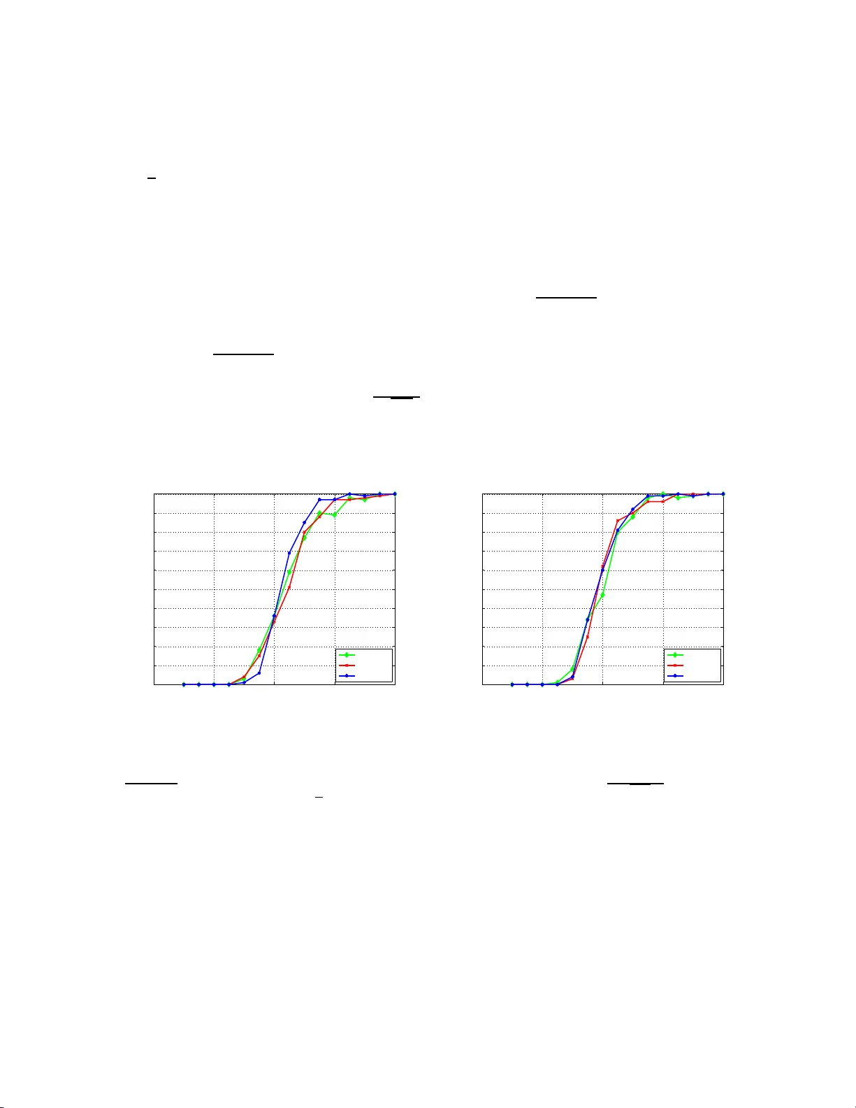
High-dimens ional subset rec o v ery in noise: Sparsified measuremen ts with out loss o f s tatistical e fficiency Dap o Omidiran ⋆ Martin J. W ain wrigh t † ,⋆ Departmen t of Statistics † , and Departmen t of Electrical Engineering and Computer Sciences ⋆ UC Berk eley , Berk eley , CA 94720 Octob er 26, 201 8 T ec hnical Rep ort, Departmen t of Statistics, UC Berkel ey Abstract W e co nsider the problem of estimating the suppor t of a vector β ∗ ∈ R p based on obser v a- tions con taminated b y noise. A significant bo dy of work has studied behavior of ℓ 1 -relaxa tions when applied to measure ment matric e s drawn from s tandard dense e ns em bles (e.g., Gaussia n, Bernoulli). In this pap er, we analyze sp arsifie d measurement ensem bles, and co nsider the trade- off betw een mea s urement s pa rsity , a s meas ured b y the fraction γ of non-z e r o e n tries , and the statistical efficiency , as mea sured by the minimal num b er of obser v ations n required for exact suppo rt recov ery with pr obability con verging to one. Our main result is to prove that it is po ssible to let γ → 0 at some rate, yielding mea s urement matrice s with a v anishing fraction of non-zeros p er row while reta ining the s ame s tatistical efficiency as dense ens em bles. A v ariety of simulation re sults c onfirm the sharpnes s of o ur theoretical predictions. Keyw ords: Quadratic pr ogramming; Lasso; subset selectio n; consistency; thresholds; sp arse ap- pro ximation; signal denoising; sparsity reco v ery; ℓ 1 -regularizatio n ; mod el selectio n 1 In tro duc tion Recen t ye ars ha ve witnessed a flu rry of researc h on th e r eco very of high-dimensional spars e sig- nals (e.g., compressed sen s ing [2, 6, 18], g r ap h ical m o del selection [13, 14], and sparse app ro xi- mation [18]). In all of these settings, the b asic p r oblem is to reco v er information ab out a high- dimensional s ignal β ∗ ∈ R p , based on a set of n observ ations. T he signal β ∗ is assu m ed a priori to b e sparse: either exactly k -sparse, or lying within some ℓ q -ball with q < 1. A large b o dy of theory has fo cused on the b ehavio r of v arious ℓ 1 -relaxatio n s when app lied to m easuremen t matrices d ra wn from the standard Gaussian ensemble [6 , 2], or more general r an d om ensem bles satisfiying mutual incoherence conditions [13, 20]. These standard random ensem bles are dense, in that the num b er of non-zero en tries p er m ea- surement vec tor is of the same order as the am bient signal dimension. Suc h dens e measuremen t matrices are un desirable for practical applications (e.g., sensor net wo rks), in w hic h it would b e preferable to take measuremen ts based on sparse inner p ro ducts. Sparse measurement matrices require significan tly less storage space, and ha v e the p oten tial for reduced algorithmic complexit y for signal reco v ery , since man y algorithms for linear programming, and conic programming more generally [1], can b e accelerate d by exploiting p roblem stru cture. With this motiv at ion, a b o dy 1 of past work (e.g . [4, 8, 16, 23]), m otiv ated by group testing or co din g p ersp ectiv es, h as studied compressed sensin g metho ds b ased on sparse measurement ensembles. How ev er, this b o dy of w ork has fo cused on the case of noiseless observ atio n s . In con trast, th is pap er fo cus es on observ ations contaminate d by additiv e noise whic h, as we sho w, exhibits fundamentall y different b eha vior than the noiseless case. Our in terest is not on sparse measurement en s em bles alone, bu t rather in un derstanding the tr ade-off b et wee n the d egree of m easuremen t s p arsit y , and its s tatistica l efficiency . W e assess m easur emen t sparsity in terms of the fraction γ of non-zero en tries in an y p articular ro w of the measur emen t matrix, and we define statistical efficiency in terms of the minimal num b er of measurements n required to reco v er the correct sup p ort with pr obabilit y con ve rging to one. Our int erest can b e view ed in terms of exp erimenta l design: more precisely w e ask: wh at degree of measuremen t sparsity can b e p ermitted without any compr omise in the statistical efficiency? T o br ing sharp fo cus to the issu e, we an alyze this qu estion for exact subset reco v ery using ℓ 1 -constrained quadratic programming, also kno wn as th e L asso in the statistics literature [3, 17], where past work on dense Gaussian measuremen t ensem bles [20] provides a pr ecise charact erization of its success/failure. W e charact erize the dens it y of our measuremen t ensembles with a p ositiv e parameter γ ∈ (0 , 1], corresp onding to the fraction of non-zero entries p er ro w. W e fi rst sho w that for all fi xed γ ∈ (0 , 1], the statistical efficiency of the Lasso remains the same as with d ense measuremen t m atrices. W e then pro ve that it is p ossible to let γ → 0 at some rate, as a function of the sample size n , signal length p and signal sparsit y k , yielding measurement matrices with a v anishing fr action of non-zero es p er ro w while requiring exactly the same n umber of observ at ions as d ense measuremen t ensem bles. In general, in contrast to the noiseless setting [23], our theory still requires that the a v erage num b er of non- zero es p er column of the measurement matrix (i.e., γ n ) tend to infin it y; h ow ev er, under the loss function consid er ed here (exact signed supp ort reco v ery), we prov e th at no metho d can succeed with p robabilit y one if this condition do es not hold. The remainder of this pap er is organized as follo ws. In Section 2 , we set up the p roblem more precisely , s tate our main r esult, and discuss s ome of its implications. In Section 3, we p ro vide a h igh-lev el outline of the pr o of. W ork in this pap er w as presen ted in part at t he International Symp osium on Information Th eory in T oron to, Canada (July , 2008 ). W e note that in concurrent and complemen tary w ork, W ang et al. [22] ha ve analyzed th e in f ormation-theoretic limitations of sparse m easuremen t matrices for exact sup p ort reco v ery . Notation: Throughout this pap er, w e use the follo wing standard asymptotic notatio n: f ( n ) = O ( g ( n )) if f ( n ) ≤ C g ( n ) for some constan t C < + ∞ ; f ( n ) = Ω( g ( n )) if f ( n ) ≥ cg ( n ) for s ome constan t c > 0; and f ( n ) = Θ( g ( n )) if f ( n ) = O ( g ( n )) and f ( n ) = Ω( g ( n )). 2 Problem set-up and main r esult W e b egin by setting u p the problem, stating our main result, and discus s ing some of their conse- quences. 2 2.1 Problem form ulation Let β ∗ ∈ R p b e a fi xed b ut unkn o wn v ector, with at most k n on-zero en tries ( k ≤ p 2 ), and define its supp ort set S := { i ∈ { 1 , . . . , p } | β ∗ i 6 = 0 } . (1) W e use β min to denote the m in im um v alue of | β ∗ | on its supp ort—th at is, β min := min i ∈ S | β ∗ i | . Supp ose that we make a set { Y 1 , . . . , Y n } of n indep endent and iden tically distributed (i.i.d.) observ atio n s of the unknown v ector β ∗ , eac h of the form Y i := x T i β ∗ + W i , (2) where W ∼ N (0 , σ 2 ) is observ at ion noise, and x i ∈ R p is a measuremen t v ector. It is conv enien t to use Y =  Y 1 Y 2 . . . Y n  T to d en ote the n -vec tor of measurements, with similar notation for the noise vec tor W ∈ R n , and X =      x T 1 x T 2 . . . x T n      =  X 1 X 2 . . . X p  . (3) to denote th e n × p measurement matrix. With this notation, the observ ation mo del can b e written compactly as Y = X β ∗ + W . Giv en some estimate b β , its error r elativ e to the tru e β ∗ can b e assessed in v arious wa ys, de- p endin g on the und erlying application of in terest. F or applications in compressed sensing, v arious t yp es of ℓ q norms (i.e., E k b β − β ∗ k q ) are well- motiv ated, whereas for statistica l p rediction, it is most natural to study a predictiv e loss (e.g., E k X b β − X β ∗ k ). F or reasons of scient ific in terpretation or for mo del selection pu rp oses, the ob j ect of primary in terest is the supp ort S of β ∗ . I n this pap er, w e consider a slightly stronger n otion of mo del selection: in particular, our goa l is to reco v er the signe d su pp ort of th e unknown β ∗ , as defin ed by the p -ve ctor S ( β ∗ ) with elements [ S ( β ∗ )] i := ( sign( β ∗ i ) if β ∗ i 6 = 0 0 otherwise. Giv en some estimate b β , we study the pr obabilit y P [ S ( b β ) = S ( β ∗ )] that it correctly sp ecifies the signed supp ort. The estimator that we analyze is ℓ 1 -constrained q u adratic programming (QP), also known as the Lasso [17] in the statistics literature. The Lasso generates an estimate b β b y s olving the regularized QP b β = arg m in β ∈ R p  1 2 n k Y − X β k 2 2 + ρ n k β k 1  , (4) where ρ n > 0 is a user-d efi ned regularization parameter. A large b o dy of past work h as fo cused on the b eha vior of the Lasso for b oth deterministic and rand om measur emen t matrices (e.g., [5, 13, 18, 20]). Most relev an t here is the sharp thresh old [20] c haracterizing the success/failure of the Lasso when applied to m easur emen t matrices X dra wn randomly from the standard Gaussian ensemble 3 (i.e., eac h elemen t X ij ∼ N (0 , 1) i.i.d.). I n particular, the Lasso un dergo es a sharp threshold as a function of the control parameter θ ( n, p, k ) := n 2 k lo g ( p − k ) . (5) F or the standard Gaussian ensemble and sequences ( n, p, k ) such that θ ( n, p, k ) > 1, the probability of Lasso success go es to one, wh ereas it con v erges to zero for sequences for whic h θ ( n, p, k ) < 1. The main cont rib ution of this pap er is to show that the same s h arp thr eshold holds for γ -sp arsified measuremen t ensembles, includ ing a subset for whic h γ → 0, so that eac h row of the measurement matrix has a v anishing fr action of non-zero entries. 2.2 Statemen t of main result A measurement matrix X ∈ R n × p dra wn randomly from a Gaussian ensem ble is dense, in that eac h ro w has Θ( p ) non-zero en tries. The main fo cus of th is pap er is the observ ation mo d el (2 ), using measuremen t ensem bles that are designed to b e sparse. T o formalize the n otion of sp arsit y , we let γ ∈ (0 , 1] represent a me asur ement sp arsity p ar ameter , corresp ondin g to the (a v erage) fraction of non-zero entries p er ro w. Our analysis allo ws the sparsit y parameter γ ( n, p , k ) to b e a f u nction of the triple ( n, p, k ), but we t ypically sup press this explicit dep endence so as to simplify notation. F or a give n c hoice of γ , we consider measurement m atrices X with i.i.d. ent ries of the form X ij d = ( Z ∼ N (0 , 1) with probabilit y γ 0 with probability 1 − γ . (6) By construction, the exp ected num b er of non-zero en tries in eac h ro w of X is γ p . It is straight - forw ard to v erify that for any constan t setting of γ , elemen ts X ij from the ensem ble (6) are sub- Gaussian. (A zero-mea n random v ariable Z is su b -Gaussian [19] if th er e exists some constant C > 0 suc h that P [ | Z | > t ] ≤ 2 exp ( − C t 2 ) for all t > 0.) F or this reason, one would exp ect suc h ensem bles to ob ey similar scaling b eha vior as Gaussian ensembles, although p ossibly with different constants. In fact, the analysis of this pap er establishes exactly the same control parameter threshold (5) for γ -sparsified measuremen t ensembles, for an y fixed γ ∈ (0 , 1), as the completely d ense case ( γ = 1). On th e other hand, if γ is allo w ed to tend to zero, elemen ts of th e measurement matrix are no longer sub-Gaussian with any fixed constan t, since the v ariance of the Gaussian mixture comp onent scales non-trivially . Nonetheless, our analysis s ho ws that for γ → 0 suitably slo wly , it is p ossible to ac hiev e the same s tatistica l efficiency as the den s e case. In p articular, we state the follo wing result on conditions u nder wh ic h the Lasso applied to spar- sified ensembles has the same sample c omp lexity as w hen applied to the dense (standard Gaussian) ensem ble: Theorem 1. Su pp ose that the me asur ement matrix X ∈ R n × p is dr awn with i.i.d. entries ac c or ding to the γ -sp arsifie d distribution (6) . Then for any ǫ > 0 , if the sample size satisfies n > (2 + ǫ ) k log( p − k ) , (7) then the L asso suc c e e ds with pr o b ability one as ( n , p , k ) → + ∞ in r e c overing the c orr e ct signe d 4 supp ort as long as nρ 2 n γ log ( p − k ) → ∞ (8a) ρ n β min 1 + √ k γ s log log( p − k ) log( p − k ) ! → 0 (8b) γ 3 min  k , log( p − k ) log log( p − k )  → ∞ . (8c) Remarks: (a) T o p ro vide int u ition for Theorem 1, it is helpful to consider v arious sp ecial cases of th e sparsit y parameter γ . First, if γ is a constant fixed to some v al u e in (0 , 1], then it pla ys no role in the scaling, and condition (8c) is alwa ys satisfied. F urthermore, condition (8a ) is then the exact same as that of from previous work [20] on dense m easur emen t ensem bles ( γ = 1). Ho w eve r, condi- tion (8b) is s ligh tly weak er than the corresp ondin g condition fr om [20] in that β min m ust approac h zero more slo wly . Dep endin g on the exact b eha vior of β min , choosing ρ 2 n to deca y slightly more slo wly than log p/n is sufficien t to guarantee exact r eco v ery with n = Θ( k lo g ( p − k )), meaning that we reco v er exactly the same statistical efficiency as the dense case ( γ = 1) f or all constan t measuremen t sparsities γ ∈ (0 , 1). At least initially , one m ight think that r ed ucing γ should in - crease the required n umber of observ ations, since it effect ively reduces the signal-to- n oise ratio by a factor of γ . Ho w ev er, und er high-dimensional scaling ( p → + ∞ ), the dominant effect limiting the Lasso p erformance is the num b er ( p − k ) of irrelev an t factors, as op p osed to the s ignal-to- n oise ratio (scaling of the minim um ). (b) Ho w eve r, Theorem 1 also allo ws f or general scalings of the measuremen t sp ars it y γ along with the tr ip let ( n, p , k ). Mo re concretely , let us supp ose for simplicit y that β min = Θ(1). Then o v er a range of signal sparsities—sa y k = αp , k = Θ( √ p ) or k = Θ(log ( p − k )), corresp ond in g resp ectiv ely to linear sparsit y , p olynomial sparsit y , and exp onent ial s p arsit y—-we can c ho ose a deca ying measuremen t s parsit y , for instance γ =  log log ( p − k ) log ( p − k )  1 6 → 0 (9) along with the regularization parameter ρ 2 n = log ( p − k ) n q log ( p − k ) log log ( p − k ) while main taining the same sample complexit y (r equ ired num b er of observ ations for sup p ort reco v ery) as the Lasso with d ense measuremen t matrices. (c) Of cour s e, the conditions of Theorem 1 do not allo w the measurement sparsity γ to approac h zero arbitrarily quic kly . Rather, for an y γ guarante eing exact reco v ery , condition (8a) implies that the a v erage n umber of non-zero en tries p er column of X (namely , γ n ) must tend to infi nit y . (Indeed, with n = Ω ( k lo g ( p − k )), our sp ecific c hoice (9) certainly satisfies this constraint.) A natural question is whether exact r eco v ery is p ossible using measuremen t matrices, either randomly d ra wn or d eterministically designed, with the a v erage n umb er of non-zeros p er ro w (namely γ n ) remaining b ound ed. I n fact, under the criterion of exactly reco v ering th e signed supp ort (4), no metho d can succeed with w .p. one if γ nβ 2 min remains b oun ded. 5 Prop osition 1. If γ nβ 2 min do es not tend to infinity, then no metho d c an r e c over the si g ne d supp ort with pr ob ability one. Pr o of. W e constru ct a sub-pr oblem that m ust b e solv able by any metho d capable of p erf orm ing exact s igned sup p ort reco v ery . Supp ose th at β ∗ 1 = β min 6 = 0 and that the column X 1 has n 1 non-zero entries, sa y w ithout loss of generalit y indices i = 1 , . . . , n 1 . No w consider the p roblem of reco v ering the sign of β ∗ 1 . Let us extract the observ atio ns i = 1 , . . . , n 1 that explicitly inv olv e β ∗ 1 , writing Y i = X i 1 β ∗ 1 + X j ∈ T ( i ) X ij β ∗ j + W i , i = 1 , . . . , n 1 where T ( i ) denotes th e set of indices in r o w i f or whic h X ij is non-zero, excluding index 1. Even assuming that { β ∗ j , j ∈ T ( i ) } were p erf ectly kn o wn, this observ ati on mo del (10) is at b est equiv alen t to observing β ∗ 1 con taminated by constan t v ariance additive Gaussian noise, and our task is to distinguish wh ether β ∗ 1 = β min or β ∗ 1 = − β min . The av erage Y = 1 n 1 P n 1 i =1 [ Y i − P j ∈ T ( i ) X ij β ∗ j ] is a sufficien t statistic, follo wing the d istribution Y ∼ N ( β min , σ 2 n 1 ). Unless the effectiv e signal-to-noise ratio, whic h is of the order n 1 β 2 min , go es to infinit y , there will alw a ys b e a constan t probabilit y of error in distinguishing β ∗ 1 = β min from β ∗ 1 = − β min . Under the γ -sp arsified r andom ensem ble, we ha ve n 1 ≤ (1 + o (1)) γ n with high probab ility , so that no metho d can su cceed u n less γ n β 2 min go es to infinity , as claimed. Note that the conditions in Th eorem 1 imply that n γ β 2 min → + ∞ . In p articular, condition (8b) implies that ρ 2 n = o ( β 2 min ), and condition (8a) implies that nγ ρ 2 n → + ∞ , whic h implies the condition of Prop osition 1. 3 Pro of of Th eorem 1 This s ection is devo ted to the pro of of Th eorem 1. W e b egin with a high-lev el outline of the pro of; as with previous work on dense Gaussian ensembles [20], the k ey is the notion of a primal-dual witness for exact signed sup p ort reco v ery . W e then pro ceed with the pro of, divided in to a sequence of separate lemmas. Analysis of “sparsified” matrices r equire results on sp ectral pr op erties of random matrices not co v ered b y the standard literature. Th e p ro ofs of some of the more tec hnical results are deferred to the app end ices. 3.1 High-lev el ov erview of pro of F or the purp oses of our pro of, it is con venien t to consider matrices X ∈ R n × p with i.i.d. ent ries of the form X ij d = ( Z ∼ N (0 , 1 γ ) with probab ility γ 0 with probability 1 − γ . (10) So as to obtain an equiv alen t observ ation mo del, we also r eset the v ariance of W i of eac h n oise term W i to b e σ 2 γ . Finally , w e can assume without loss of generalit y that sign( β ∗ S ) = ~ 1 ∈ R k . 6 Define the sample c ovarianc e matrix b Σ := 1 n X T X = 1 n n X i =1 x i x T i . (11) Of particular imp ortance to our analysis is the k × k sub-matrix b Σ S S . F or futu r e reference, we state the follo wing claim, prov ed in App endix D: Lemma 1. U nder the c onditions of The or em 1 , the submatrix b Σ S S is invertible with pr ob ability gr e ater than 1 − O ( 1 ( p − k ) 2 ) . The foundation of ou r pr o of is the follo wing lemma: it pro vides su fficien t conditions for the Lasso (4) to r eco v er the signed su pp ort set. Lemma 2 (Primal-dual conditions for supp ort reco v ery) . Supp ose that b Σ S S ≻ 0 , and that we c an find a primal ve ctor b β ∈ R p , and a sub gr a dient ve ctor b z ∈ R p that satisfy the zero-subgradient condition b Σ  β ∗ − b β  + 1 n X T W + ρ n b z = 0 , (12) and the signed-sup p ort-reco v ery conditions b z i = sign( β ∗ i ) for al l i ∈ S , (13a) b β j = 0 for al l j ∈ S c , (13b) | b z j | < 1 for al l j ∈ S c , and (13c) sign( b β i ) = sign( β ∗ i ) for al l i ∈ S . (13d) Then b β is the unique optimal solution to the L asso (4) , and r e c overs the c o rr e ct signe d supp ort. See App endix B.1 for the pro of of this claim. Th u s, given Lemmas 1 and 2, it su ffices to sho w that under the s p ecified scaling of ( n, p, k ), there exists a pr imal-dual pair ( b β , b z ) satisfying the conditions of Lemma 2. W e establish the existence of suc h a pair with the follo wing constructive pro cedure: (a) W e b egin by setting b β S c = 0, and b z S = sign( β ∗ S ). (b) Next we determine b β S b y solving the linear s ystem b Σ S S  β ∗ S − b β S  + 1 n X T S W + ρ n sign( β ∗ S ) = 0 . (14) (c) Finally , w e determine b z S c b y solving the linear s ystem: − ρ n b z S c = b Σ S c S  β ∗ S − b β S  + 1 n X T S c W . (15) 7 By construction, this p ro cedure satisfies the zero sub-gradient condition (12 ), as wel l as auxiliary conditions (13a) and (13b); it r emains to v erify conditions (13c) an d (13d). In order to complete these final tw o steps, it is helpf ul to defin e the follo wing random v ariables: V a j := 1 n X T j n X S ( b Σ S S ) − 1 ~ 1 o ρ n (16a) V b j := X j T  1 n X S ( b Σ S S ) − 1 X T S − I n × n  W n , (16b) U i := e T i  b Σ S S  − 1  1 n X T S W − ρ n ~ 1  , (16c) where e i ∈ R k is the u n it v ector with one in p osition i , and 1 ∈ R k is the all-ones v ector. A little bit of algebra (see App en dix B.2 for details) sho ws that ρ n b z j = V a j + V b j , and that U i = b β i − β ∗ i . C onsequen tly , if w e define the ev ents E ( V ) :=  max j ∈ S c | V a j + V b j | < ρ n  (17a) E ( U ) :=  max i ∈ S | U i | ≤ β min  , (17b) where the min imum v alue β min w as d efined previously as the minimum v alue of | β ∗ | on its su pp ort, then in order to establish that the L asso succeeds in reco v ering the exact signed supp ort, it suffi ces to sho w that P [ E ( V ) ∩ E ( U )] → 1, W e decomp ose th e pro of of this fi nal claim in the follo wing thr ee lemmas. As in the statemen t of Theorem 1, supp ose that n > (2 + ǫ ) k log( p − k ), for some fixed ǫ > 0. Lemma 3 (Control of V a ) . Under the c onditio ns of The or em 1, we have P [max j ∈ S c | V a j | ≥ (1 − δ ) ρ n ] → 0 . (18) Lemma 4 (Control of V b ) . Under the c onditions of The or em 1, we have P [max j ∈ S c | V b j | ≥ δ ρ n ] → 0 . (19) Lemma 5 (Control of U ) . Under the c ond itions of The or em 1 , we have P [( E ( U )) c ] = P [max i ∈ S | U i | > β min ] → 0 . (20) 3.2 Pro of of Lemma 3 W e assume through ou t that b Σ S S is inv ertible, an ev ent whic h o ccurs with p robabilit y 1 − o (1) und er the stated assu mptions (see Lemma 1 ). If we define the n -dimensional v ector h := X S ( b Σ S S ) − 1 ~ 1 , (21) then the v ariable V a j can b e wr itten compactly as V a j ρ n = X T j h = n X ℓ =1 h ℓ X ℓj . (22) 8 Note that eac h term X ℓj in this sum is distributed as a mixture v ariable, taking the v alue 0 with probabilit y 1 − γ , and d istributed as N (0 , 1 γ ) v ariable with probabilit y γ . F or eac h ℓ = 1 , . . . , n , define the discr ete random v ariable H ℓ d = ( h ℓ with p robabilit y γ 0 with p robabilit y 1 − γ . (23) F or eac h index ℓ = 1 , . . . , n , let Z ℓj ∼ N (0 , 1 γ ). With these defin itions, by construction, we ha ve V a j ρ n d = n X ℓ =1 H ℓ Z ℓj . T o gain some in tuition for the b eha vior of this sum, note that th e v ariables { Z ℓj , ℓ = 1 , . . . , n } are indep end en t of { H ℓ , ℓ = 1 , . . . , n } . (In particular, eac h H ℓ is a function of X S , wher eas Z ℓj is a function of X ℓj , w ith j / ∈ S .) Consequent ly , we ma y condition on H w ithout affecting Z , and since Z is Gaussian, we ha ve ( V a j ρ n | H ) ∼ N (0 , k H k 2 2 γ ). Therefore, if we can obtain go o d control on the norm k H k 2 , then w e can u se standard Gaussian tail b oun ds (see App endix A) to con trol the maxim um m ax j ∈ S c V a j /ρ n . The follo wing lemma is p ro v ed in App endix C: Lemma 6. Under c ond ition (8c) , then for any fixe d δ > 0 , we have P  k H k 2 2 ≤ γ k (1 + δ ) n  ≥ 1 − O (exp( − min { 2 log ( p − k ) , n 2 k } )) The primary imp lication of the ab ov e b ound is that eac h V a j /ρ n v ariable is (essen tially) n o larger than a N (0 , k n ) v ariable. W e can then use standard techniques for b oundin g th e tails of Gaussian v ariables to obtain go o d con trol o ve r the rand om v aria b le max j ∈ S c | V a j | /ρ n . In particular, by union b ound , we hav e P [max j ∈ S c | V a j | ≥ (1 − δ ) ρ n ] ≤ ( p − k ) P [ n X ℓ =1 H ℓj Z j ≥ (1 − δ )] F or an y δ > 0, d efine the ev ent T ( δ ) := {k H k 2 2 ≤ k γ (1+ δ ) n } . Cont inuing on, we h a v e P [max j ∈ S c | V a j | ≥ (1 − δ ) ρ n ] ≤ ( p − k ) ( P [ n X ℓ =1 H ℓj Z j ≥ (1 − δ ) | T ( δ )] + P [( T ( δ ) c )] ) ≤ ( p − k )  2 exp  − n (1 − δ ) 2 2 k (1 + δ )  + O (exp( − min (2 log ( p − k ) , n 2 k )))  , where the last line uses a standard Gaussian tail b ou n d (see App endix A), and Lemma 6. Finally , it can b e v erified th at un der the condition n > (2 + ǫ ) k log ( p − k ) for s ome ǫ > 0, and with δ > 0 c hosen sufficien tly small, w e hav e P [max j ∈ S c | V a j | ≥ (1 − δ ) ρ n ] → 0 as claimed. 9 3.3 Pro of of Lemma 4 Defining the orth ogonal pro jection matrix Π ⊥ S := I n × n − X S ( X T S X S ) − 1 X T S , we then ha v e P [max j ∈ S c | V b j | ≥ δ ρ n ] = P [max j ∈ S c   X T j Π ⊥ S ( W /n )   ≥ δ ρ n ] ≤ ( p − k ) P h   X T 1 Π ⊥ S ( W /n )   ≥ δ ρ n i . (24) Recall from equation (23 ) the represent ation X ℓ 1 = H ℓj Z ℓj , w here H ℓj is Bernoulli with pa- rameter γ , and Z ℓj ∼ N (0 , 1 γ ) is Gaussian. The v ariable P n ℓ =1 H ℓj is b inomial; d efi ne the follo wing ev en t T := ( 1 n   n X ℓ =1 H ℓj − γ n   ≤ 1 2 √ k ) . F rom th e Ho effding b ound (see Lemma 7), w e ha ve P [ T c ] ≤ 2 exp ( − n 2 k ). Using this representat ion and conditioning on T , we h a v e P h   X T j Π ⊥ S ( W /n )   ≥ δ ρ n i ≤ P "   1 n n X ℓ =1 H ℓj Z ℓj Π ⊥ S ( W ) ℓ   ≥ δ ρ n | T # + P [ T c ] ≤ P      1 n n ( γ + 1 2 √ k ) X ℓ =1 Z ℓj Π ⊥ S ( W ) ℓ   ≥ δ ρ n    + 2 exp( − n 2 k ) , where w e h a v e assumed without loss of generalit y th at the fi rst n ( γ + 1 2 √ k ) elemen ts of H are non-zero. Since Π ⊥ S is an orthogonal pro jection matrix, w e h av e k Π ⊥ S ( W ) k 2 ≤ k W k 2 , so that P h   X T j Π ⊥ S ( W /n )   ≥ δ ρ n i ≤ P      1 n n ( γ + 1 2 √ k ) X ℓ =1 Z ℓj W ℓ   ≥ δ ρ n    + 2 exp( − n 2 k ) , (25) Conditioned on W , the r andom v ariable M j := 1 n P n ( γ + 1 2 √ k ) ℓ =1 Z ℓj W ℓ is zero-mean Gaussian with v ariance ν ( W ; γ ) := 1 n 2 γ n ( γ + 1 2 √ k ) X ℓ =1 W 2 ℓ . F or some δ 1 > 0, defin e the ev en t T 2 ( δ 1 ) :=  ν ( W ; γ ) ≤ (1 + δ 1 ) σ 2 nγ 2 ( γ + 1 2 √ k )  . Note th at E [ ν ( W ; γ )] = σ 2 nγ 2 ( γ + 1 2 √ k ). Since γ σ 2 P n ( γ + 1 2 √ k ) ℓ =1 W 2 ℓ is χ 2 with d = n ( γ + 1 2 √ k ) d egrees of freedom, u sing χ 2 -tail b ounds (see App en d ix A), we ha v e P [( T 2 ( δ 1 )) c ] ≤ exp  − n ( γ + 1 2 √ k ) 3 δ 2 1 16  . 10 No w, b y conditioning on T 2 ( δ 1 ) and its complemen t and using tail b ounds on Gaussian v ariate s (see App en dix A), w e obtain P      1 n n ( γ + 1 2 √ k ) X ℓ =1 Z ℓj W ℓ   ≥ δ ρ n    ≤ P      1 n n ( γ + 1 2 √ k ) X ℓ =1 Z ℓj W ℓ   ≥ δ ρ n | T 2 ( δ 1 )    + P [( T 2 ( δ 1 )) c ] ≤ 2 exp − nγ 2 ( δ 2 ρ 2 n ) 2 σ 2 (1 + δ 1 )( γ + 1 2 √ k ) ! + exp  − n ( γ + 1 2 √ k ) 3 δ 2 1 16  . (26) Finally , putting together th e pieces fr om equations (26), (25), and equation (24), w e obtain that P [max j ∈ S c | V b j | ≥ δ ρ n ] is up p er b oun ded by ( p − k ) ( 2 exp ( − n 2 k ) + 2 exp − nγ 2 ( δ 2 ρ 2 n ) 2 σ 2 (1 + δ 1 )( γ + 1 2 √ k ) ! + exp  − n ( γ + 1 2 √ k ) 3 δ 2 1 16  ) . The first term go es to zero s ince n > (2 + ǫ ) k log( p − k ). The second term goes to zero b ecause ev en tually γ 2 γ + 1 2 √ k > γ 2 (b ecause C ondition (8c) implies that γ √ k → ∞ ), and Conditon (8a) implies that C nγ ρ 2 n − log ( p − k ) → ∞ . Our choice of n an d Condition (8c) (whic h implies that γ k → ∞ ) is enough f or the third term goes to zero. 3.4 Pro of of Lemma 5 W e first observe that conditioned on X S , eac h U i is Gaussian w ith mean and v ariance: m i := E [ U i | X S ] = e T i  1 n X T S X S  − 1  − ρ n ~ 1  , ψ i := v ar[ U i | X S ] = σ 2 γ n e T i  1 n X T S X S  − 1 e i Define the u p p er b ound s m ∗ := ρ n (1 + √ k O ( 1 γ s max  log ( k ) k log ( p − k ) , log log( p − k ) log( p − k )  )) ψ ∗ := σ 2 γ n " 1 − O ( 1 γ s max  log ( k ) k log ( p − k ) , log log( p − k ) log( p − k )  ) # − 1 and the follo wing ev ent T ( m ∗ , ψ ∗ ) := { max i ∈ S | m i | ≤ m ∗ and max i ∈ S | ψ i | ≤ ψ ∗ } . Conditioning on T and its complemen t, w e ha v e P [( E ( U )) c ] = P [ 1 β min max i ∈ S U i | > 1] ≤ P [ 1 β min max i ∈ S | U i | > 1 | T ( m ∗ , ψ ∗ )] + P [( T ( m ∗ , ψ ∗ )) c ] . 11 Applying Lemma 10 with t = 1 and θ = k , we h a v e P [( T ( m ∗ , ψ ∗ )) c ] ≤ k O ( k − 2 ). W e n ow deal with the first term. Letting Y i ∼ N (0 , ψ i ), and using T as sh orth and for the ev en t T ( m ∗ , ψ ∗ ), w e h a v e P [ 1 β min max i ∈ S | U i | > 1 | T ] = E  P  max i ∈ S | U i | > β min | X S , T   ≤ E  P  max i ∈ S  | m i | + | Y i |  > β min | X S , T   ≤ E  P  m ∗ + max i ∈ S | Y i | > β min | X S , T   = E  P  1 β min max i ∈ S | Y i | > 1 − m ∗ β min | X S , T   . Condition (8b) imp lies that m ∗ β min → 0, so th at it suffices to u pp er b ound E  P  1 β min max i ∈ S | Y i | > 1 2 | X S , T   ≤ E  k P [ | Y ∗ | ≥ β min 2 | X S , T ]  ≤ 2 k exp  − β 2 min 8 ψ ∗  . where Y ∗ ∼ N (0 , ψ ∗ ), and we hav e us ed stand ard Gaussian tail b ounds (see App endix A). It remains to v erify th at this fi nal term con v erges to zero. T aking logarithms and ignoring constan t terms, w e ha v e log ( k )(1 − β 2 min log( k ) 8 ψ ∗ ) = log ( k )     1 − β 2 min γ n  1 − O ( 1 γ r max n log ( k ) k log ( p − k ) , log log( p − k ) log( p − k ) o )  8 σ 2 log k     . W e w ould lik e to show that this qu an tit y div erges to −∞ . Condition (8c) implies that 1 γ s max  log ( k ) k log ( p − k ) , log log( p − k ) log( p − k )  → 0 . Hence, it suffi ces to sho w that log k  1 − β 2 min γ n 16 σ 2 log k  div erges to −∞ . W e ha ve log( k )  1 − β 2 min γ n 16 log ( k )  = log( k ) (1 − β 2 min ρ 2 n γ nρ 2 n 16 σ 2 log( k ) ) = log( k ) (1 − β 2 min ρ 2 n γ nρ 2 n 16 σ 2 log( p − k ) log( p − k ) log ( k ) ) Condition (8b) implies that β 2 min ρ 2 n → ∞ and Condition (8a) states that γ nρ 2 n log( p − k ) → ∞ . In our observ atio n mo del, k ≤ p 2 , and so the third term is greater than one. Therefore, we hav e that P [ E ( U ) c ] tends to zero. 12 4 Exp erimen tal Results In this section, w e p ro vide s ome exp erimental results to illustrate the claims of Th eorem 1. W e consider t wo differen t sparsity regimes, namely linear sp ars it y ( k = αp ) and p olynomial sparsity ( k = √ p ), and we allo w γ to con verge to zero at some rate. F or all exp erimen ts, the additiv e noise v ariance is set to σ 2 = 0 . 0625 and we fix the v ector β ∗ b y setting the fir st k entries are set to one, and the remaining en tries to zero. Th ere is no loss of generalit y in fixing the su pp ort in this w a y , since the ensemble in in v arian t under p ermutatio ns . Based on Lemma 2 , it su ffi ces to simulate the rand om v ariables { V a j , V b j , j ∈ S c } and { U i , i ∈ S } , and th en chec k th e equiv alen t conditions (17a) and (17b). In all cases, w e plot th e su ccess proba- bilit y P [ S ( b β ) = S ( β ∗ )] ve rsu s the c ontr ol p ar ameter θ ( n, p, k ) = n 2 k log ( p − k ) . Note th at Theorem 1 predicts that the Lasso should transition from failure to su ccess for θ ≈ 1. In Figure 1, the empirical su ccess rate of the Lasso is p lotted against the cont rol parame- ter θ ( n, p, k ) = n 2 k log ( p − k ) . Eac h panel sho ws three cu rv es, corresp onding to the problem sizes p ∈ { 512 , 1024 , 2048 } , and eac h p oint on the curve represen ts the a verag e of 100 trials. F or the exp eriments in Figure 1, we s et γ = 0 . 5 log ( p − k ) √ p − k , which con v erges to zero at a rate slightl y faster than th at guaran teed b y Theorem 1. Nonetheless, we still observe the ”stac king” b eha vior aroun d the pr edicted th reshold θ ∗ = 1. 0 0.5 1 1.5 2 0 0.1 0.2 0.3 0.4 0.5 0.6 0.7 0.8 0.9 1 Control parameter Prob. of success Polynomial signal sparsity; Decaying γ p = 512 p = 1024 p = 2048 0 0.5 1 1.5 2 0 0.1 0.2 0.3 0.4 0.5 0.6 0.7 0.8 0.9 1 Control parameter Prob. of success Linear signal sparsity; Decaying γ p = 512 p = 1024 p = 2048 (a) (b) Figure 1. Plots o f the success probability P [ b S = S ] versus the control parameter θ ( n, p, k ) = n k log( p − k ) for γ -s parsified ensembles, with decaying measur ement sparsity γ = . 5 log ( p − k ) √ p − k . (a) Poly- nomial signal spar sity k = O ( √ p ). (b) Linear signal spars it y k = Θ ( p ). 5 Discussion In this p ap er, w e hav e stud ied the p roblem of reco ve r y the supp ort set of a sparse v ector β ∗ based on noisy obs erv ati ons. Th e m ain result is to sh o w that it is p ossible to “sp arsify” standard d en se measuremen t matrices, so that they hav e a v anishing fraction of n on-zero es p er r o w, wh ile retaining the same samp le complexit y (num b er of observ ations n ) required for exact reco very . W e also sho wed 13 that u n der the su pp ort reco very m etric and in the p resence of noise, no metho d can succeed without the num b er of non-zero es p er column tending to in finit y . S ee also the pap er [22] for complement ary results on the information-theoretic scaling of sparse measurement ensembles. The approac h tak en in this p ap er is to find rates whic h γ (as a fun ction of n , p , k ) can safely tend to w ards zero while main taining the same statistical efficiency as dense r andom matrices. In v arious practical settings [21], it m a y b e p r eferable to mak e th e measuremen t ensem bles eve n spars er at the cost of taking more measurement s n and th us decreasing efficiency relativ e to dense random matrices. A n atural qu estion is the sample complexit y n ( γ , p, k ) in this regime as w ell. Finally , th is w ork h as focus ed only on a r andomly sparsified matrices, as opp osed to particular spars e d esigns (e.g., b ased on LDPC or expand er-t yp e constructions [7, 16, 23]). Although our resu lts imply that exact supp ort reco v ery with noisy observ ations is im p ossible with b ound ed degree designs, it w ould b e in teresting to examine the trade-off b et wee n other loss fu nctions (e.g, ℓ 2 reconstruction error) and sparse m easur emen t d esigns. Ac knowled gmen ts This work was partially s u pp orted by NS F grant s CAREER-CCF-0545862 and DMS-06051 65, a V o d afone-US F oundation F ello wship (DO), an d a Sloan F oundation F ello wship (MJW). A Standard concen tration results In this app endix, w e collec t some tail b ound s used r ep eatedly throughout th is pap er. Lemma 7 (Ho effding b ound [9]) . Given a binomial variate Z ∼ Bin( n, γ ) , we have for any δ > 0 P [ | Z − γ n | ≥ δ n ] ≤ 2 exp  − 2 nδ 2  . Lemma 8 ( χ 2 -concen tration [10]) . L et X ∼ χ 2 m b e a chi-squ ar e d variate with m de gr e e s of fr e e dom. Then for al l 1 2 > δ ≥ 0 , we have P [ X − m ≥ δ m ] ≤ exp  − 3 16 mδ 2  . W e will also fi nd the follo wing standard Gaussian tail b ound [11] u seful: Lemma 9 (Gaussian tail b eha vior) . L et V ∼ N (0 , σ 2 ) b e a zer o-me an Gaussian with varianc e σ 2 . Then for al l δ > 0 , we have P [ | V | > δ ] ≤ 2 exp  − δ 2 2 σ 2  . B Con v ex optimalit y conditions B.1 Pro of of Lemma 2 Let f ( β ) := 1 2 n k Y − X β k 2 2 + ρ n k β k 1 denote the ob j ective fun ction of the L asso (4) . By standard con v ex optimalit y conditions [15], a v ector b β ∈ R p is a solution to th e Lasso if and only if 0 ∈ R p is an element of the su b differential of f ( β ) at b β . These conditions lead to 1 n X T ( X b β − Y ) + ρ n b z = 0 , 14 where the du al vecto r b z ∈ R p is an element of the su b differential of the ℓ 1 -norm, giv en b y ∂ k b β k 1 = n z ∈ R p | z i = sign( b β i ) if b β i 6 = 0 , z i ∈ [ − 1 , 1] otherwise o . No w supp ose that we are giv en a pair ( b β , b z ) ∈ R p × R p that satisfy the assu mptions of Lemma 2. Condition (12) is equiv alen t to ( b β , b z ) satisfying the zero subgradient condition. Cond i- tions (13a), (13c) and (13d) ensu re that b z is an elemen t of th e sub d ifferen tial of the ℓ 1 -norm at b β . Finally , conditions (13b) and (13d) ensure that b β correctly sp ecifies the signed supp ort. It remains to v erify that b β is the unique optimal solution. By Lagrangian d ualit y , th e Lasso problem (4) (giv en in p enalized f orm) can b e wr itten as an equ iv al ent constrained optimization problem ov er the ball k β k 1 ≤ C ( ρ n ), for some constan t C ( ρ n ) < + ∞ . Equiv alen tly , w e can express this single ℓ 1 -constrain t as a set of 2 p linear constraint s ~ v T β ≤ C , one for eac h sign v ector ~ v ∈ {− 1 , +1 } p . The v ector b z can b e written as a con v ex combinatio n b z = P ~ v α ∗ ~ v ~ v , w h ere th e w eigh ts α ∗ ~ v are n on-negativ e and su m to one. By construction of b β and b z , the w eigh ts α ∗ form an optimal Lagrange m ultiplier v ector for the pr oblem. C onsequen tly , any other optimal solution—say e β —m ust also minimize the asso ciated Lagrangian L ( β ; α ∗ ) = f ( β ) + X ~ v α ∗ ~ v  ~ v T β − C  , and s atisfy th e complementary slac kness conditions α ∗ ~ v  ~ v T e β − C  = 0. Note that th ese comple- men tary slac kness conditions imply th at b z T e β = C . But th is can only h app en if e β j = 0 f or all indices where | b z j | < 1. Th erefore, an y optimal solution e β satisfies e β S c = 0. Fin ally , giv en that all optimal solutions satisfy β S c = 0, we m a y consider the restricted optimization problem sub ject to this set of constrain ts. If the Hessian submatrix b Σ S S is strictly p ositiv e definite, then this sub -problem is strictly con vex, so that b β m ust b e the uniqu e optimal solution, as claimed. B.2 Deriv at ion of { V a j , V b j , U i } In this app endix, w e derive the form of th e { V a j , V b j } and { U i } v ariables defined in equations (16a ) through (16c). W e b egin b y writing the zero sub -gradien t condition in a blo c k-form, and substi- tuting the relations sp ecified in conditions (13a) and (13b): " b Σ S S b Σ S S c b Σ S c S b Σ S c S c #  b β S − β ∗ S 0  +  1 n X T S W 1 n X T S c W  + ρ n  sign( β ∗ S ) b z S c  = 0 . By solving th e top blo ck, we obtain U := b β S − β ∗ S = − b Σ − 1 S S  1 n X T S W + ρ n sign( β ∗ S )  . By b ac k-substituting th is r elation into th e low er blo c k, we can solv e explicitly f or b z S c ; doing so yields that b z S c = V a + V b , wher e th e ( p − k )-vec tors are d efined in equations (16a ) and (16b). 15 C Pro of of Lemma 6 Let Z ∈ R n × n denote a n × n matrix, for whic h the off-diagonal elements Z ij = 0 for all i 6 = j , and the diagonal element s Z ii ∼ Ber( γ ) are i.i.d. With this notation, we can write H d = Z h . Using the definition (21) of h , w e h a v e k H k 2 2 = k Z h k 2 2 = k Z X S n ( b Σ S S ) − 1 ~ 1 k 2 2 = ~ 1 T ( b Σ S S ) − 1 ( Z X S n ) T ( Z X S n )( b Σ S S ) − 1 ~ 1 = γ n ~ 1 T ( b Σ S S ) − 1 ( 1 γ n n X i =1 I [ Z ii = 1] x i x T i ) | {z } ( b Σ S S ) − 1 ~ 1 Γ( Z ) where x i is the i th ro w of th e matrix X S . F rom Lemma 10 with θ = 1 and t = ( p − k ), we hav e P h | | | b Σ − 1 S S | | | 2 ≥ f 1 ( p, k, γ ) i ≤ 1 ( p − k ) 2 (27) where f 1 ( p, k, γ ) :=  1 − O  1 γ r max n 1 k , log log( p − k ) log( p − k ) o  − 1 . Next we con trol the sp ectral norm of the random matrix Γ( Z ), cond itioned on the total n umb er P n i =1 Z ii of non -zero en tries. In particular, applying Lemma 10 with t = p − k , and θ = 1, we ha ve P " k Γ Z k 2 ≥ z nγ  1 + C z n s max  1 k z n , log z n log( p − k ) z n log( p − k )   | n X i =1 Z ii = z # ≤ 1 ( p − k ) 2 , (28) as long as k z n → ∞ . The next step is to deal with the conditioning. Define the ev en t T ( k , γ ) := ( Z | γ − 1 √ 2 k ≤ 1 n n X i =1 Z ii ≤ γ + 1 2 √ k ) . Defining the f u nction f 2 ( p, k, γ ) := 1 + 1 2 √ k γ ! " 1 + O  1 γ v u u t max ( 1 k ( γ − 1 2 √ k ) , log ( γ + 1 2 √ k ) log( p − k ) ( γ − 1 2 √ k ) log( p − k ) )  # , w e ha v e P [ | | | Γ( Z ) | | | 2 ≥ f 2 ( p, k, γ )] ≤ P [ | | | Γ( Z ) | | | 2 ≥ f 2 ( p, k, γ ) | T ( k, γ )] + P [( T ( k , γ )) c ] ≤ exp( − 2 log( p − k )) + 2 exp( − n 2 k ) ≤ 3 exp( − min { 2 log ( p − k ) , n 2 k } ) , (29) 16 where we h av e used the b ound (28), and the Ho effding b ound (see Lemm a 7). Com binin g th e b ou n ds (27) and (29), we conclude th at as long as γ k → ∞ , then: P h | | | b Σ − 1 Γ( Z ) b Σ − 1 | | | 2 ≥ f 2 1 f 2 i ≤ 4 exp( − min { 2 log ( p − k ) , n 2 k } ) . Since k ~ 1 k 2 = √ k , we ha v e P [ k H k 2 2 ≥ γ k n f 2 1 f 2 ] ≤ 4 exp( − min { 2 log ( p − k ) , n 2 k } ) . T o conclud e the pro of, we note that assumption (8c) implies that b oth f 1 ( p, k, γ ) and f 2 ( p, k, γ ) con v erge to 1 as ( p, k , γ ) scale. In particular, f or an y fixed δ > 0, we hav e f 2 1 f 2 < (1 + δ ) for ( p, k ) sufficien tly large, so that Lemma 6 follo ws. D Singular v alues of sparsified matrices Let θ ( p, k ) ∈ (0 , 1] and t ( p, k ) ∈ { 1 , 2 , 3 , . . . } b e functions. Let X b e an θ n × k rand om matrix with i.i.d. en tries X ij distributed according to the γ -sp arsified ensemble (6). Lemma 10. Supp o se that n ≥ (2 + ν ) k lo g ( p − k ) for some ν > 0 . If as k , p − k , → ∞ T ( γ , k , p , θ , t ) := 1 γ s max  log ( t ) θ k log ( p − k ) , log[ θ log( p − k )] θ log ( p − k )  − → 0 then for some c onstan t C ∈ (0 , ∞ ) , we have P " sup k u k 2 =1   1 √ θ n k X u k 2 − 1   ≥ C T ( γ , k , p, θ , t ) # ≤ O ( 1 t 2 ) , (30) Note that Lemma 10 with θ = 1 and t = p − k implies that b Σ = 1 n X T S X S is inv ertible with probabilit y greater than 1 − O ( 1 ( p − k ) 2 ), there establishing Lemma 1. O th er settings in w h ic h this lemma is applied are ( θ , t ) = ( γ , p − k ) and ( θ , t ) = (1 , k ). The r emainder of this s ection is dev oted to the p ro of of Lemma 10. D.1 Bounds on exp ect ed v alues Let X ∈ R θ n × k b e a rand om matrix w ith i.i.d. en tries, of the sparsified Gaussian form X ij ∼ (1 − γ ) δ X (0) + γ N (0 , 1 γ ) . Note that E [ X ij ] = 0 an d v ar( X ij ) = 1 by construction. W e follo w the pro of tec hn ique outlined in [19]. W e first note the tail b oun d: Lemma 11. L et Y 1 , . . . , Y d b e i. i .d. samples of the γ -sp arsifie d ensemble. Given any ve ctor a ∈ R d and t > 0 , we have P [ P d i =1 a i Y i > t ] ≤ exp  − γ t 2 2 k a k 2 2  . 17 T o establish this b oun d, note that eac h Y i is d ominated (sto c hastically) by the rand om v ariable Z ∼ N (0 , 1 γ ). In particular, w e hav e M Y i ( λ ) = E [exp( λY i )] = (1 − γ ) + γ E [exp( λZ )] ≤ exp( λ 2 / 2 γ ) . No w let us b ound the maximum singular v alue s k ( X ) of the rand om matrix X . Letting S d − 1 denote the ℓ 2 unit ball in d dimensions, we b egin with the v aria tional represent ation s k ( X ) = max u ∈ S k − 1 k X u k = max v ∈ S θn − 1 max u ∈ S k − 1 v T X u. F or an arbitrary ǫ ∈ (0 , 1), w e can fin d ǫ -co v ers (in ℓ 2 norm) of S θ n − 1 and S k − 1 with M θ n ( ǫ ) = (3 /ǫ ) θ n and M k ( ǫ ) = (3 /ǫ ) k p oint s resp ectiv ely [12]. Denote these co ve r s b y C θ n ( ǫ ) and C k ( ǫ ) resp ectiv ely . A standard argument sho ws that for all ǫ ∈ (0 , 1), w e h av e k X k 2 ≤ 1 (1 − ǫ ) 2 max u α ∈ C k ( ǫ ) max v β ∈ C θn ( ǫ ) v T β X u α . Let us analyze the maxim um on th e RHS: for a fixed pair ( u, v ) in our cov ers, we h a v e u T X v = θ n X i =1 k X j =1 X ij u i v j . Let us app ly Lemma 11 with d = θ nk , and w eigh ts a ij = u i v j . Note that we ha ve k a k 2 2 = = X i,j a 2 ij = X i u 2 i ( X j v 2 j ) = 1 since eac h u and v are unit norm. Consequently , for an y fi x ed u, v in the co ve rs, we h a v e P [ u T X v > t ] ≤ exp  − γ t 2 2  By the un ion b ound , we hav e P  max u α ∈ C k ( ǫ ) max v β ∈ C θn ( ǫ ) v T β X u α > t  ≤ M k ( ǫ ) M θ n ( ǫ ) exp  − γ t 2 2  ≤ exp  ( k + θ n ) log(3 /ǫ ) − γ t 2 2  . By c ho osing ǫ = 1 2 and t = q 4 γ ( k + θ n ) log 6, we can conclude that s 1 ( X ) / √ θ n = k X k 2 / √ θ n ≤ C r 1 γ r 1 + k θ n w.p. 1 − exp( − ( k + θ n ) log 6). Note that k θ n = O  1 (2 + ν ) θ l og ( p − k )  → 0 , 18 since log[ θ l og( p − k )] θ log ( p − k ) → 0, which implies that θ lo g ( p − k ) → ∞ . Consequent ly , w e can conclude that k X k 2 / √ θ n ≤ O (1 / √ γ ) w.p. one as θ n, k → ∞ . Although this b oun d is essen tially correct f or a N (0 , 1 γ ) en sem ble with γ fixe d , it is v ery crude for the sparsified case with γ → 0, but w ill usefu l in obtaining tigh ter con trol on s 1 ( X ) and s k ( X ) in the sequ el. D.2 Tigh tening the b ound F or a giv en u ∈ S k − 1 , consid er the random v ariable k X u k 2 2 := P θ n i =1 ( X u ) 2 i . W e first claim that eac h v a r iate Z i = ( X u ) 2 i is sub exp onent ial: Lemma 12. F or any t > 0 , we have P [ Z i > t ] ≤ 2 exp  − γ t 2  . Pr o of. W e can write ( X u ) i = P k j =1 X ij u j where k u k 2 = 1. Hence, fr om Lemma 11, w e ha v e P [ k X j =1 X ij u j > δ ] ≤ exp( − γ δ 2 2 ) . By symmetry , we ha v e P [ Z i > t ] = P [ | P k j =1 X ij u j | > √ t ] ≤ 2 exp( − γ t 2 ) as claimed. No w consid er the ev ent P      k X u k 2 2 θ n − 1     > δ  = P "      θ n X i =1 Z i − E [ θ n X i =1 Z i ]      > δθ n # W e may apply Theorem 1.4 of V ershynin [19] with b = 8 θ n/γ 2 and d = 2 /γ . Hence, we hav e 4 b/d = 16 θ n/γ , w hic h grows at least linearly in θ n . Hence, f or an y δ > 0 less than 16 θ n/γ (w e will in fact tak e δ → 0), we hav e P      k X u k 2 2 θ n − 1     > δ  ≤ 2 exp − δ 2 ( θ n ) 2 256 θn /γ 2 ! = 2 exp  − γ 2 δ 2 θ n 256  . No w take an ǫ -co v er of th e k -dimensional ℓ 2 ball, sa y with N ( ǫ ) = (3 /ǫ ) k elemen ts. By union b ound , we hav e P  inf i =1 ,...,N ( ǫ ) k X u i k 2 2 θ n < 1 − δ  ≤ exp  − γ 2 δ 2 θ n 256 + k lo g (3 /ǫ )  No w set δ = √ 2 γ r 256 f ( k , p ) k log (3 /ǫ ) θ n , where f ( k , p ) ≥ 1 is a fun ction to b e sp ecified. Doing so yields that the infi mum is b ounded b y 1 + δ w ith probabilit y 1 − exp ( − k f ( k , p ) log (3 /ǫ )). (Note that the c hoice of f ( k , p ) influ ences th e rate of conv ergence, h ence its utilit y .) 19 F or an y element u ∈ S k − 1 , w e ha v e some u i in the cov er, and moreo v er   k X u k 2 − k X u i k 2   = |{k X u k − k X u i k} {k X u k + k X u i k}| ≤ | {k X u k − k X u i k}| (2 k X k ) ≤ ( k X k k u − u i k ) (2 k X k ) ≤ 2 k X k 2 ǫ F rom our earlier result, we kno w that k X k 2 = O ( θ n/γ ) with p robabilit y 1 − exp(log 6( k + θ n )). Putting together the pieces, w e ha v e that the b ound 1 θ n inf u ∈ S k − 1 k X u k 2 ≥ 1 + δ + C 2 ǫ/γ = 1 + 2 γ r 32 f ( k, p ) k log(3 /ǫ ) θ n + C 2 γ ǫ, for some constant C 2 > 0 ind ep endent of θ n, k , γ , h olds with pr obabilit y at least min { 1 − exp( − k f ( k , p ) log(3 /ǫ )) , 1 − exp( − log 6( k + θ n )) } , (31) No w set ǫ = 3 k /θ n , so that w e h av e w.h .p . 1 θ n inf u ∈ S k − 1 k X u k 2 ≥ 1 − C 3 γ r f ( k , p ) k θ n log( θ n k ) (Note that we h a v e u tilized the fact that b oth q f ( k , p ) k θ n log( θ n k ) and k θ n → 0, bu t th e former more slo wly th an the latter.) Since k /θ n → 0, this qu an tit y will go to zero, as long as f ( k , p ) remains fixed, or scales slo wly enough. T o und erstand h o w to c ho ose f ( k , p ), let us consider the rate of con v ergence (31). T o establish th e claim (30), we need r ates fast enough to dominate a log ( t ) term in the exp onen t, whic h guid es our choic e of f ( k , p ). Recall that we are seeking to prov e a scaling of the form n = Θ ( k log ( p − k )), so that our requirement (with ǫ = 3 k/θ n = 3 θ log ( p − k ) ) is equ iv ale nt to the quan tit y k f ( k , p ) log (3 /ǫ ) − log( t ) = k f ( k , p ) log [ θ log( p − k )] − log( t ) tending to infinit y . First, if k > log( t ) log[ θ l og( p − k )] , then w e ma y simp ly set f ( k , p ) = 2. O therwise, if k ≤ log( t ) log θ l og( p − k ) , then we may set f ( k , p ) = 2 log( t ) k log θ log ( p − k ) ≥ 1 . If f ( k , p ) = 2, then w e hav e f ( k , p ) k θ n log( θ n k ) = 2 log[ θ log( p − k )] θ log ( p − k ) → 0 . In the other case, if k ≤ log( t ) log θ l og( p − k ) , w e ha v e f ( k , p ) k θ n log( θ n k ) ≤ 2 log( t ) k log θ log ( p − k ) 1 θ log ( p − k ) log θ log( p − k ) = 2 k log t θ log ( p − k ) → 0 , 20 whic h again follo ws f rom the assumptions in Lemma 10. Recalling the d efinition of T ( γ , k , p, θ , t ) from Lemma 10, we can su m marize b oth cases can b e summarized cleanly by sa ying that with pr obabilit y greater than 1 − 1 t 2 : 1 θ n inf u ∈ S k − 1 k X u k 2 ≥ 1 − C γ s max  1 k log t θ lo g ( p − k ) , log θ log( p − k ) θ log ( p − k )  = 1 − C T ( γ , k , p, θ , t ) Because T ( γ , k, p, θ , t ) → 0, for all p ≥ p ∗ 1 , k ≥ k ∗ 1 , C T ( γ , k , p, θ , t ) < 1. Thus we can tak e squ are ro ot of b oth sides and apply th e identit y √ 1 + x = 1 + x 2 + o ( x ) (v alid for | x | < 1) to conclude that, with probability greater than 1 − C 1 ( p ∗ 1 ,k ∗ 1 ) t 2 : 1 √ θ n inf u ∈ S k − 1 k X u k ≥ 1 − C 2 T ( γ , k , p , θ , t ) + o ( T ( γ , k , p, θ , t )) , As T ( γ , k , p, θ , t ) → 0, for all k ≥ k ∗ 2 , p ≥ p ∗ 2 w e ha v e that | o ( T ( γ , k , p, θ , t )) | < C 4 T ( γ , k , p , θ , t ) Th u s, with probab ility greater than 1 − C 2 ( p ∗ 1 ,k ∗ 1 ,p ∗ 2 ,k ∗ 2 ) t 2 : 1 √ θ n inf u ∈ S k − 1 k X u k ≥ 1 − 3 C 4 T ( γ , k , p , θ , t ) , Note that this same pro cess can b e rep eated to b ound th e maxim um singular v alue, yielding the follo wing result: 1 √ θ n sup u ∈ S k − 1 k X u k ≤ 1 + 3 C 4 T ( γ , k , p , θ , t ) , Com binin g th ese t wo b oun ds, we h a v e pro ved Lemma 10. References [1] S. Bo yd and L. V andenb erghe. Convex optimization . Cambridge Univ ersity Press, Cambridge, UK, 2004. [2] E. Cand es and T. T ao. Decodin g by linear pr ogramming. IEEE T r ans. Info The ory , 51(12 ):4203–421 5, Decem b er 2005. [3] S. Chen, D. L. Donoho, and M. A. Saunders. A tomic decomp osition by b asis pu r suit. SIAM J. Sci. Computing , 20(1):33– 61, 1998 . [4] G. Commo de and S. Muthukrishnan. T o wards an algo r ith m ic theory of compressed s ensing. T echnical rep ort, Ru tgers Univ ersit y , Ju ly 2005. [5] D. Donoho. F or most large und erdetermined systems of linear equations, the minimal ℓ 1 -norm near-solution app ro ximates the sparsest n ear-solution. Communic ations on Pur e and Applie d Mathematics , 59(7):907 –934, July 2006. 21 [6] D. Donoho. F or most large und erdetermined systems of linear equations, the minimal ℓ 1 -norm solution is also the s p arsest solution. Communic ations on P ur e and Applie d Mathematics , 59(6): 797–829, Ju ne 2006. [7] J. F eldman, T. Malkin, R. A. Serv edio, C. Stein, and M. J. W ain wr igh t. LP deco ding corrects a constan t fraction of errors . IEE E T r ans. Informatio n The ory , 53(1):82–8 9, Jan uary 200 7. [8] A. Gilber t, M. S trauss, J. T ropp , and R. V ershynin. Algorithmic linear dim en sion reduction in the ℓ 1 -norm for sparse vec tors. In Pr o c. Al lerton Confer enc e on Communic ation, Contr ol and Computing , Allerton, IL, S eptem b er 2006 . [9] W. Ho effding. Probability inequalities for su ms of b ounded random v ariables. Journal of the Americ an Statistic al Asso c iation , 58:13–30 , 1963 . [10] I. J ohnstone. Chi-square oracle inequalities. In M. de Gu nst, C. Klaassen, an d A. v an der V aart, editors, State of the A rt i n Pr ob ability and Statistics , num b er 37 in IMS Lecture Notes, pages 399–418 . Institute of Mathematical S tatistics, 2001. [11] M. Ledoux and M. T alagrand. Pr ob ability in Banach Sp ac es: Isop erimetry and Pr o c esses . Springer-V erlag, New Y ork, NY, 1991. [12] J. Matousek. L e ctur es on discr e te ge om etry . Springer-V erlag, New Y ork, 2002 . [13] N. Meinshausen and P . Buhlmann . High-dimensional graphs and v ariable selection with th e lasso. A nnals of Statistics , 2006 . T o app ear. [14] P . Ravikumar, M. J. W ain wr igh t, and J. Laffert y . High-dimen sional graph selection using ℓ 1 - regularized logistic regression. T ec hnical Rep ort 750, UC Berk eley , Department of Statistic s, April 2008. Po sted at http://a rXiv.org/abs/0804.4 2 02; Conference version app eared at NIPS Conference, Decem b er 2006. [15] G. Ro ck afellar. Convex Analysis . P r inceton Unive rs it y Pr ess, Princeton, 197 0. [16] S. Sarvo tham, D. Baron, and R. G. Baraniuk. Sud o co des: F ast measurement and reconstruc- tion of sparse s ignals. In Int. Symp osium on Information The ory , Seattle, W A, J u ly 2006. [17] R. Tibsh ir ani. Regression shrink age and selection via the lasso. Journal of the R o yal Statistic al So c iety, Series B , 58(1):267 –288, 1996 . [18] J. T r opp. Just relax: Conv ex pr ogramming metho d s for identifying sparse signals in noise. IEEE T r ans . Info The or y , 52(3):1030 –1051, Marc h 2006 . [19] R. V ershynin. On large random almost euclidean bases. A cta. Math. U niv. Comenianae , LXIX:137–1 44, 2000. [20] M. J. W ainwrigh t. Sh arp thresh olds for high-dimensional and noisy r eco v ery of sparsity using using ℓ 1 -constrained qu adratic p rograms. T ec hnical Rep ort 709, Departmen t of Statistics, UC Berk eley , 2006. [21] M. B. W akin, J. N. Lask a, M. F. Duarte, D. Baron, S. Sarvo tham, D. T akh ar, K. F. Kelly , and R. G. Baraniuk. An arc hitecture for compressiv e imaging. IEEE Int. Conf. Image Pr o c. , pages 1273–12 76, 8-11 Oct. 2006. 22 [22] W. W ang, M. J. W ainwrigh t, and K. Ramchandran. In formation-theoretic limits on sparse su p- p ort reco v ery: Dense versus sparse measurements. T echnical r ep ort, Departmen t of Statistics, UC Berk eley , April 2008. S hort v ersion present ed at In t. S ymp. Info. T heory , J uly 2008. [23] W. Xu and B. Hassib i. Efficien t compressiv e sensing with d eterministic guarante es us ing expander graphs . Information The ory Workshop, 2007. ITW ’ 07. IEEE , p ages 414–4 19, 2-6 Sept. 2007. 23