On Emergence of Dominating Cliques in Random Graphs

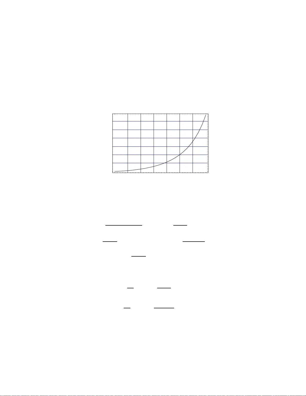
On Emergence of Dominating Cliques in Random Graphs Martin Neh ´ ez Department of Information T ec hn ologies, VSM School of Management, City Universit y of Seattle, P an´ onsk a cesta 17, 851 0 4 Bratisl av a, Slov ak Republic e-mail: mnehez@vsm.sk Daniel Olej´ ar Department of C omput er Science, FMPI, Comenius Universit y in Bratis lav a, Mlynsk´ a dolina, 842 4 8 Bratisl av a, Slov ak Republic Mic hal Demetrian Department of Mathematical and N u merical An alysis, FMPI, Co menius Universit y in Bra tislav a, Mlynsk´ a dolina M 105, 842 4 8 Bratisl av a, Slov ak Republic No v em b er 20, 2021 Abstract Emergence of dominating cliques in Erd¨ o s-R´ enyi random graph mod el G( n, p ) is in vestigated in this pap er. It is shown this p henomenon p os- sesses a phase transition. Namely , we hav e argued that, giv en a con- stant probabilit y p , an n -n od e random graph G from G( n, p ) and for r = c log 1 /p n with 1 ≤ c ≤ 2, it holds: (1) if p > 1 / 2 then an r -no de clique is dominating in G almost surely and, (2) if p ≤ (3 − √ 5) / 2 th en an r -no de clique i s not dominating in G almo st surely . The remaining range of probability p is discussed with more attention. A detailed stud y sho ws that this problem is answ ered b y examination of sub-logarithmic gro wth of r u p on n . Keywords: Rand om graphs, dominating cliques, phase transiti on. 1 1 In tro duc tion The phase transition pheno menon w as or iginally obs e rved as a physical effect. In dis crete mathematics, it was origina lly describ ed b y P . E rd¨ os a nd A. R´ enyi in [8]. The most frequently prop erty of gr aphs which have been studied with relation to the phase transitions in random gr aphs is the connectivity . The recent surveys o f known results concerning this area can b e find in Refs. [2] and [9], Chapter 5. Our pap er deals with a no ther int ere s ting gra ph problem that is the emerging of a dominating clique in a r andom gra ph. The theory o f dominating cliques in rando m graphs has se veral nontrivial applications in computer sc ie nce. The most sig nificant ones a re: (1) heuristics in satisfiability search [5] and (2) the construction of a space- e fficie nt interv a l ro uting scheme with a small additive stretch for almo st all and large-sca le distributed sy stems [13]. 1.1 Preliminaries and terminology Given a graph G = ( V , E ), a set S ⊆ V is s aid to be a dominating set of G if each no de v ∈ V is either in S or is adjac ent to a node in S . The domination numb er γ ( G ) is t he minimum cardinality o f a dominating set of G . A clique in G is a maximal set of mutually a djacent node s of G , i.e., it is a maximal complete subgra ph of G . The clique nu mb er , denoted cl ( G ), is the nu mber of no des of clique of G . If a subgraph S induced b y a dominating s e t is a clique in G then S is called a dominating clique in G . The mo del of rando m graphs is introduced in the following wa y . Let n b e a p ositive integer and let p ∈ I R, 0 ≤ p ≤ 1, b e a pr ob ability of an e dge . The (pr ob abilistic) mo del of r andom gr aphs G( n, p ) consists of a ll gra phs with n -no de set V = { 1 , . . . , n } such that ea ch graph has at mos t  n 2  edges b eing inserted independently with probability p . Conse quently , if G is a gr aph with no de set V and it has | E ( G ) | edges, then a pr obability measur e Pr defined o n G( n, p ) is given by: Pr[ G ] = p | E ( G ) | (1 − p ) ( n 2 ) −| E ( G ) | . This model is also called Er d¨ os-R ´ enyi r andom gra ph mo del [2, 9]. Let A b e any set of gr aphs from G( n, p ) with a pro p e rty Q . W e say that almost al l gr aphs ha ve the proper ty Q iff: Pr[ A ] → 1 as n → ∞ . The term ”a lmost surely” stands for ”with the probability a pproaching 1 as n → ∞ ” . 2 1.2 Previous work and our result Dominating sets and cliq ue s ar e basic structures in g raphs and they hav e b een inv estigated very int ensively . T o determine whether the domination num b er of a gra ph is at most r is an NP-complete problem [6]. The maximum-clique problem is one o f the first shown to b e NP-ha rd [11]. A well-kno wn result of B. Bollo b´ as, P . Erd¨ os et al. states that the clique num b er in random graphs G( n, p ) is b o unded by a very tight b ounds [2, 3, 10, 1 2, 15, 16]. Let b = 1 / p and let r 0 = lo g b n − 2 log b log b n + log b 2 + log b log b e , (1) r 1 = 2 log b n − 2 log b log b n + 2 log b e + 1 − 2 lo g b 2 . (2) J. G. Ka lbfleisch and D. W. Matula [10, 12] proved that a random gr aph from G( n, p ) do es not contain cliques of the order greater than ⌈ r 1 ⌉ and less or equal than ⌊ r 0 ⌋ almos t surely . (See a lso [3, 15, 16].) The domination num b er of a random graph hav e been studied by B. W ieland a nd A. P . Go db ole in [17]. The phase transition of domina ting clique problem in random g raphs was studied indep endently by M. Neh´ ez and D. Olej´ ar in [13, 14] and J. C. Culb e r son, Y. Gao, C. Anton in [5 ]. It was shown in [5] that the prop er t y of having a dominating c liq ue is monotone, it has a phase tr ansition a nd the corresp onding threshold pr obability is p ∗ = (3 − √ 5) / 2. The standa rd firs t and the second moment methods (base d on the Marko v’s and the Chebyshev’s inequa lities, resp ectively , see [1, 9]) were used to pro ve this result. Ho wev er, the preliminary result of M. Neh ´ ez and D. Olej´ ar [14] pointed out that to complete the behavior of r andom g raphs in all sp e c tra of p needs a more accurate analysis, namely in the cas e when (3 − √ 5) / 2 < p ≤ 1 / 2. The main r e sult of this pa p er is the refinement of the pr e vious results from [5, 13, 14]. Le t us formulate this as the following theor e m. Theorem 1 L et 0 < p < 1 b e fixe d and let I L x denote lo g 1 / (1 − p ) x . L et r b e or der of a clique such that ⌊ r 0 ⌋ ≤ r ≤ ⌈ r 1 ⌉ . L et δ ( n ) : I N → I N b e an arbitr ary slow ly incr e asing function such that δ ( n ) = o (log n ) and let G ∈ G( n, p ) b e a r andom gr aph. Then: 1. If p > 1 / 2 , t hen an r - no de clique is dominating in G almost su r ely; 2. If p ≤ (3 − √ 5) / 2 , then an r -no de clique is not dominating in G almost sur ely; 3. If (3 − √ 5) / 2 < p ≤ 1 / 2 , then an r -n o de clique: • is dominating in G almost sur ely, if r ≥ I L n + δ ( n ) , • is not dominating in G almost sur ely, if r ≤ I L n − δ ( n ) , • is dominating with a finite pr ob ability f ( p ) for a su itable function f : [0 , 1 ] → [0 , 1 ] , if r = I L n + O (1) . 3 T o prov e Theo r em 1 the first and the second moment metho d w ere used. The leading part of o ur analysis follows from a prop erty o f a function defined as a ratio of t wo ra ndo m v a r iables which count domina ting cliques and all cliques in ra ndom graphs, resp ectively . The critical v alues of p : (3 − √ 5) / 2 and 1 / 2, resp ectively , are obtained from the bo unds (1), (2) see [10, 12]. The rest of this pap er contains the pro of of the Theor em 1. Section 2 contains the preliminary results. An ex pe c ted num ber of dominating cliques in G( n, p ) is estimated here. The main result is prov ed in s e ction 3. Possible applications are discussed in section 4. 2 Preliminary results F or r > 1, let S be an r -no de s ubset of an n -no de graph G . Let A denote the even t that ” S is a dominating clique of G ∈ G( n, p )” . Let in r be the associa ted 0-1 (indica to r) r andom v ariable on G( n, p ) defined as follows: in r = 1 if G contains a dominating cliq ue S and i n r = 0, otherw is e. Let X r be a ra ndom v a riable that denotes the n umber of r - no de dominating cliques. More prec isely , X r = P in r where the summation range s ov er all sets S . The following lemma expresses the exp ectation of X r . Lemma 1 [13] The exp e ctation E ( X r ) of the r andom variable X r is given by: E ( X r ) =  n r  p ( r 2 ) (1 − p r − (1 − p ) r ) n − r . (3) W e use the following prop erties adopted from [15], pp. 501–5 02. Claim 1. L et 0 < p < 1 and k ≤ ( η − 1) ln n ln p , η < 0 starting with some p ositive inte ger n . Then: (1 − p k ) n = exp( − np k )  1 + O ( np 2 k )  = 1 − np k + O  np 2 k  . Claim 2. L et k = o ( √ n ) , then: n k = n ( n − 1 ) · · · ( n − k + 1) = n k  1 −  k 2  1 n + O  k 4 n 2  . The upper b ound o n r in G( n, p ) is stated in the following lemma. Lemma 2 L et b = 1 /p and r u = 2 log b n − 2 log b log b n + 2 log b e + 1 − 2 lo g b 2 . ( 4) A r andom gr aph fr om G( n, p ) do es not c ontain dominating cliques of the or der gr e ater than r u with pr ob ability appr o aching 1 as n → ∞ . 4 Remark 1 Note that the upp er b ounds r u and r 1 ar e the same. The ar gument for estimation of r 1 is t he same as in L emma 2. T o o bta in co nditions for an existence of dominating cliques in ra ndo m gra phs it is sufficien t to es timate the v a riance V ar ( X r ). W e can use the fact that the clique num ber in r andom graphs lyes down in a tight in terv al. W e use the bo unds (1) and (2) due to [1 0, 12]. The estimatio n of the v ariance V ar ( X r ) is stated in the following lemma. Lemma 3 L et p b e fixe d, 0 < p < 1 and ⌊ r 0 ⌋ ≤ r ≤ ⌈ r 1 ⌉ . L et β = min { 2 / 3 , − 2 log b (1 − p ) } . Then: V ar ( X r ) = E ( X r ) 2 · O  (log n ) 3 n β  . (5) The following claim e x presses the num be r o f the do minating cliques in ran- dom graphs. Lemma 4 L et p , r and β b e as b efor e, and X r =  n r  p ( r 2 ) (1 − p r − (1 − p ) r ) n − r ×  1 + O  (log n ) 3 n β / 2  . (6) The pr ob ability that a r andom gr aph fr om G( n, p ) c ont ains X r dominating cliques with r no des is 1 − O  (log n ) − 3  . 3 Pro of of Theorem 1 F or r > 1, let Y r be the random v ariable on G( n, p ) which denotes the num ber of r -no de cliques . According to [15], Y r =  n r  p ( r 2 ) (1 − p r ) n − r ×  1 + O  (log n ) 3 √ n  . (7) The ratio X r / Y r expresses the relative n umber of do minating cliques (with r no des) to all cliques (with r no des) in G( n, p ) and it attains a v alue in the int erv al [0, 1]. By analysis of the as ymptotic of X r / Y r as n tends ∞ w e obtain our main result. Let us examine the limit v a lue of the ratio X r / Y r : X r Y r =  1 − p r − (1 − p ) r 1 − p r  n − r × ×  1 + O  (log n ) 3 √ n  ×  1 + O  (log n ) 3 n β / 2  . (8) 5 The most impo rtant term of the expre ssion (8) is the first one, since the la st t wo terms tend to 1 as n → ∞ . Let us define α : [0 , 1] → I R b y: α ( p ) = − log 1 /p (1 − p ) . The plot of its graph is in fig. 1 and for the simplification, we will wr ite also α instead of α ( p ). Note that (1 − p ) r = p r α . (9) 0 0.1 0.2 0.3 0.4 0.5 0.6 0.7 p 0 0.5 1 1.5 2 2.5 3 Α H p L Figure 1: The graph of the function α ( p ) = − log 1 /p (1 − p ). According to Claim 1 and (9) w e hav e:  1 − p r − (1 − p ) r 1 − p r  n − r =  1 − p r α 1 − p r  n − r = = exp  − np r α 1 − p r  ·  1 + O  np 2 r α  ·  1 + O  (log n ) 2+ α n  = = exp  − np r α 1 − p r  ·  1 + O  np 2 r α  . Let us a nalyze the asymptotic b ehavior of the ratio X r / Y r as n tends to ∞ . According to the assumption n → ∞ , w e can write X r / Y r in the following t w o equiv a lent forms : X r Y r = ex p  − np r α 1 − p r  , or, applying (11), as: X r Y r = exp  − n (1 − p ) r 1 − p r  . Using b ounds (1) and (2), the admissible num ber of no des of a clique r depends on n as (w e consider the leading term only): r = ρ log b n, (10) 6 where 1 ≤ ρ ≤ 2. This results in: X r Y r = exp  − n 1 − ρα 1 − p r  , and one has three differen t cas e s: 1. 1 − ρα < 0 , ∀ ρ ∈ [1 , 2] ⇔ p > 1 2 , 2. 1 − ρα ≥ 0 , ∀ ρ ∈ [1 , 2] ⇔ p ≤ 3 − √ 5 2 , 3. 1 − ρα changes sig n as ρ v ar ie s in [1 , 2] ⇔ 3 − √ 5 2 < p ≤ 1 2 . The first case implies lim n →∞ X r Y r = 1 , that means the r − no de cliques is do minating in G almost s urely . The second case implies lim n →∞ X r Y r = 0 , and therefore a r − no de clique is not dominating in G almost surely . In the third case, there exists a v alue o f ρ (for eac h p ) in the in terv al [1 , 2]: ˆ ρ = 1 α ( p ) , for which we ha ve: r = ˆ ρ lo g b n = log 1 / (1 − p ) n and lim n →∞ X r Y r = exp ( − n (1 − p ) r ) = e − 1 . The ratio X r / Y r approaches 1 (0) for ρ > ˆ ρ ( ρ < ˆ ρ ). Due to corrections of or der less than Θ(log n ) to the equation (10) taken with ρ = ˆ ρ the v alue o f e − 1 to b e changed to another cons ta nt greater or equal than 0 and less o r equal tha n 1. The details ar e given her e . Let δ ( n ) : I N → I N b e an incr easing function s uch that δ ( n ) = o (log n ). If r = ˆ ρ log b n + δ ( n ), then X r / Y r approaches 1 as exp  − (1 − p ) δ ( n )  . If r = ˆ ρ log b n − δ ( n ), then X r / Y r approaches 0 as exp  − (1 − p ) − δ ( n )  . And finally , if r differs from ˆ ρ log b n by a constant λ , then the ratio X r / Y r asymptotically lo oks like exp( − (1 − p ) λ ). The pro of is complete. ♦ 7 0 20 40 60 80 n 0 0.2 0.4 0.6 0.8 X r  Y r Figure 2: The plot of the fractio n X r / Y r versus n for three different c hoices of ρ in the in termediate ca s e when 3 − √ 5 2 < p ≤ 1 2 . In all three cases p is set to b e 0 . 45 and ρ v aries (from the top to the botto m) a s: ρ = 1 . 9, ρ = 1 /α (0 . 45), and finally ρ = 1 . 05. 4 Discussion W e have cla imed the conditions for the existence of dominating cliques in E rd¨ os- R ´ enyi random graph mo del. Our result is the r efinement of the pre v ious ones from [5, 13, 14]. F or p ossible applications of this result w e address the tw o w or ks o f J. C. Culber son, Y. Gao , C. Anton [5] a nd M. Neh´ ez and D. Olej´ ar [13]. The pa p e r [5] deals w ith heuristics in satisfiability search. F o r the sec o nd applicatio n, describ ed in [13], we mention the cons tr uction of a space-efficient interv a l routing scheme with a small additive stre tch in almost all netw ork s mo delled by rando m graphs G( n, p ) where p > 1 / 2. An a pplica tion of this result ca n b e found in decentralized cont ent sharing s ystems based on the p eer-to-p ee r (shortly P2P ) paradigm such as F reenet whic h us es the idea of interv a l ro uting for retrie ving files from loca l datastores according to keys [4]. Ac kno wledgem en t. This work ha s b een s upp o r ted by Gr atex Resear ch, Bratislav a, by CU grant No. 40 3/20 07 and by the VEGA gran t No. 1/304 2/06. References [1] N. Alon, J . Sp encer: The pr ob abilistic met ho d (2nd e dition) , John Wiley & Sons, New Y or k, 2000. [2] B. Bollo b´ as: Ra ndom Gr aphs (2nd e dition) , Cambridge Studies in Adv anced Mathmatics 73, 2001. 8 [3] B. Bollo b´ as, P . Er d¨ os: Cliques in r andom gr aphs , Math. Pro c. Cam. Phil. So c. (1976), 80, pp. 419– 4 27. [4] L. Bononi: A Persp e ctive on P2P Par adigm and Servic es , Slide co urtesy of A. Montresor, URL: htt p://w ww.cs .unibo.it/people/faculty/bononi/ /AdI20 04/Ad I11.pdf [5] J. C. Culb er son, Y. Gao, C. Anton: Phase T r ansitions of D ominating Clique Pr oblem and Their Implic ations t o Heuristics in S atisfiability Se ar ch , In Pro c. 19th In t. Joint Conf. on Artificial In telligence, IJCAI 200 5, 7 8 –83. [6] M. R. Garey , D.S. Johnso n: Computers and Intr actability , F reeman, New Y or k, 1979. [7] J. L. Gross, J. Y ellen: H andb o ok of Gr aph The ory , CR C Press, 2003 . [8] P . Erd¨ os, A. R´ enyi: On the evolution of r andom gr aphs , P ubl. Math. Inst. Hungar. Acad. Sci., 5 (1960), pp. 17–61 . [9] S. J anson, T. Luczak , A. Rucinski: R andom Gr aphs , John Wiley & Sons , New Y or k, 2000. [10] J . G. Kalbfleisch: Complete sub gr aphs of r andom hyp er gr aphs and bip artite gr aphs , In P ro c. 3 rd Southea stern Co nf. of Combinatorics, Graph Theo r y and Computing, Florida At lantic Univ ersity , 1972 , pp. 297–3 04. [11] R. M. Karp: R e ducibili ty among c ombinatorial pr oblems , In Complexity of Computer Co mputation, (R. E. Miller and J. W. Thatcher, eds.), Plenum Press, 1972, 24, pp. 85–10 3. [12] D. W. Matula: The lar gest clique size in a r andom gr aph , T echnical rep ort CS 7608, Dept. of Comp. Sci. Southern Methodist University , Dallas, 1976. [13] M. Neh ´ ez, D. Ole j´ ar: An Impr ove d Interval Routing Scheme for A lmost Al l Networks Base d on Dominating Cliques , In Pro c. 16th Int. Symp o s ium on Algorithms and Computation, ISAAC 2005, Springer Berlin-Heidelb erg, LNCS 3827/ 2005 , 52 4 –532 . [14] M. Neh´ ez, D. Olej´ ar : On Dominating Cliques in R andom Gr aphs , Research Repo rt, KAM-Dimatia Series 200 5-750 , Charles Univ ers it y , Prag ue, 2005. [15] D. Olej´ ar, E . T oman: On the Or der and the Numb er of Cliques in a R andom Gr aph , Math. Slov a ca, 47(5), 1997, pp. 499–510 . [16] E . M. Palmer: Gr aphic al Evolution , John Wiley & So ns, Inc., New Y ork , 1985. [17] B. Wieland, A. P . Go db ole: On the Domination N umb er of a R andom Gr aph , Electronic Journal of Com binator ics, 8(1), #R37, 2001. 9 App endix Pro of of Lemma 2. The pro of follows from the Ma rko v’s inequalit y [9], p. 8: Pr[ X ≥ t ] ≤ E ( X ) t , t > 0 . Let us denote α = lo g 1 /p  1 1 − p  = − log b (1 − p ). Note that: (1 − p ) r = p r α . (11) Let r = (2 − ε ) lo g b n , where 0 ≤ ε < 1 . Accor ding to Claim 1 we hav e three cases: p > 1 / 2 , p = 1 / 2 and p < 1 / 2 . The first tw o of them ca n b e a na lyzed together, p erforming element ar y computations w e obtain: (1 − p r − (1 − p ) r ) n − r ≈ 1 − n ǫ − 1 → n →∞ 1 , if p ≥ 1 2 . In the case p < 1 / 2 the same kind of a lgebra shows th at (1 − p r − (1 − p ) r ) n − r ≈ exp h − n 1 − (2 − ǫ ) ln(1 − p ) ln( p ) i , if p < 1 2 . W e distinguish tw o different a symptotics in the pre v ious formula. F or given p < 1 / 2 they are separ ated b y the condition 1 − (2 − ˆ ǫ ) ln(1 − p ) ln( p ) = 0 . This is solved with resp ect to ˆ ǫ as: ˆ ǫ = 2 − ln( p ) ln(1 − p ) . Now we ha ve: • for ǫ > ˆ ǫ (1 − p r − (1 − p ) r ) n − r → 0 as n → ∞ , • for ǫ < ˆ ǫ (1 − p r − (1 − p ) r ) n − r → 1 as n → ∞ , With resp ect to upp er and lower bo und on size of a domina ting clique we req uire ǫ ra nges b etw een 0 a nd 1. This re quirement defines then tw o critica l v alues o f the probability p : • ˆ ǫ = 1 - in this case p = 1 2 , 10 • ˆ ǫ = 0 - in this case p = 3 − √ 5 2 . The Stirling’s formula (e.g. [16], p. 127) yields to:  n r  p ( r 2 ) ∼  nep ( r − 1) / 2 r  r . (12) Consequently ,  n r u  p ( r u 2 ) → 1 and  n r u + 1  p ( r u +1 2 ) ∼ log b n n → 0 The rest follows from the Markov’s inequality (4) f or t = 1. ♦ Pro of of Lemma 3. In order to prov e this lemma w e will estimate the v a riance of X r : V ar ( X r ) = E ( X 2 r ) − E 2 ( X r ) . (13) The expectatio n of X 2 r can be ex pressed in the following way: E ( X 2 r ) = r X j =0  n r  r j  n − r r − j  · p 2 ( r 2 ) − ( j 2 ) × × (1 − p r − (1 − p ) r ) 2 n − 4 r +2 j · Pr[ S 1 r , S 2 r ] . (14) The equation (14) follows from the next analys is. The no des o f the first dom- inating clique S 1 r can b e c hosen in  n r  wa ys. The dominating cliques S 1 r , S 2 r can (but need not to) ha ve j commo n nodes. These no des can be c hose n in  r j  wa ys. The remaining ( r − 1) no des of the second dominating clique S 2 r hav e to b e chosen from ( n − r ) no des of V ( G ) \ V ( S 1 r ). Now w e shall c ho os e edges: bo th dominating c liq ues ar e r -no de co mplete gr aphs and therefor e they co nt ain 2  r 2  edges. But S 1 r , S 2 r can hav e a nonempty in tersec tio n - a complete j -no de subgraph. Therefore  j 2  edges were coun ted twice. Bo th subgraphs S 1 r , S 2 r are dominating cliques a nd so all n − 2 r + j nodes of the set V ( G ) \ [ V ( S 1 r ) ∪ V ( S 2 r )] are ”g o o d” with resp ect to b oth S 1 r , S 2 r . The last ter m, Pr[ S 1 r , S 2 r ] denotes the probability that the no des of V ( S 1 r ) \ V ( S 2 r ) are go od with respe ct to S 2 r and the no des of V ( S 2 r ) \ V ( S 1 r ) are go o d with resp ect to S 1 r . It is s ufficie nt to estimate Pr[ S 1 r , S 2 r ] b y 1. T o prove that V a r ( X r ) is asymptotically less than E 2 ( X r ), we extract the expression E 2 ( X r ) in front of the sum stated by the equation (14). W e have: E ( X 2 r ) ≤ E 2 ( X r ) · r X j =0  n r  − 1  r j  n − r r − j  · p − ( j 2 ) · Q ( p, r, j ) , (15) 11 where Q ( p, r, j ) = (1 − p r − (1 − p ) r ) − 2 r +2 j . First w e estimate the expression Q ( p, r, j ). Let us denote α = − log b (1 − p ), as befo r e. Recall that (1 − p ) r = p r α . Let us also denote: ν = min { 1 , − log b (1 − p ) } . (16) Therefore, from ⌊ r 0 ⌋ ≤ r ≤ ⌈ r 1 ⌉ (cf. [15]), Claim 1 and (11), it follows: Q ( p, r, j ) < [1 − p r 0 − p αr 0 ] − 2 r ≤ ≤  1 − (log b n ) 2 2 n · log b e −  (log b n ) 2 2 n · log b e  α  − 4 log b n = = ex p  4 log b n ·  (log b n ) 2 2 n · log b e +  (log b n ) 2 2 n · log b e  α  × × 1 + O (log n ) 1+2 ν n 2 ν !! = = exp  2(log b n ) 3 n · log b e  · exp  4(log b n ) 2 α +1 (2 n · log b e ) α  ·  1 + O  (log n ) 1+2 ν n 2 ν  , where ν = min { 1 , α } . Since 2(log b n ) 3 n · lo g b e → 0 and 4(log b n ) 2 α +1 (2 n · log b e ) α → 0 as n → ∞ , the v alue of Q ( p, r , j ) is 1 + o (1) or, more precis ely: Q ( p, r, j ) = 1 + O  (log n ) 2 ν +1 n 2 ν  . (17) Now we can concent ra te our effort o n the estimation of the sum r X j =0  n r  − 1  r j  n − r r − j  · p − ( j 2 ) , (18) where: ⌊ r 0 ⌋ ≤ r ≤ ⌈ r 1 ⌉ . W e use a similar approach as D. Olej´ ar and E. T oman in [15], pp. 50 4–50 6 . This sum w as also estimated in Subsection 5.3. of [16] (pp. 77– 80), but w e need more accurate calculation here. First we in tro duce the following notation: S ( n, r , c, d ) = d X j = c  n r  − 1  r j  n − r r − j  · b ( j 2 ) . 12 Our s olution is based on the idea to divide the sum S ( n, r, a, b ) in to three parts by the following w ay: S ( n, r , 0 , r ) ≤ S ( n, r, 0 , 1) + S ( n, r, 2 , r 2 ) + S ( n, r , r 2 , r ) , (19) where: r 2 = (1 + λ ) log b n for 0 < λ < 1 . All these three parts will b e estimated separately . Using Claim 2, the first part is estimated as follows: S ( n, r , 0 , 1) =  n − r r  n r  − 1 + r ·  n − r r − 1  n r  − 1 = =  1 − r 2 n   1 + O  (log n ) 4 n 2  + r 2 n + O  (log n ) 3 n 2  = = 1 + O  (log n ) 4 n 2  . (20) T o estimate the second part, it is s ufficient to analyze the binomial co e fficie nts. (See also [16], pp. 79–80 .)  n r  − 1  r j  n − r r − j  = r ! n r · r j j ! · ( n − r ) r − j ( r − j )! = = r j · ( r − j )! ( r − j )! · r j j ! · ( n − r ) r − j n j · ( n − j ) r − j ≤ r j · r j j ! · n j ≤ r 2 j j ! · n j ∼ r 2 j j ! · n j W e use the Stirling’s formula in the follo wing form: j ! ∼  j e  j . Consequently ,  n r  − 1  r j  n − r r − j  · b ( j 2 ) ∼  r 2 · b j / 2 · e j · n · √ b  j . ( 21 ) The mem b ers of the sum S ( n, r, 2 , r 2 ) attain their asymptotic maximum for j = r 2 . More precisely , letting j = r 2 = (1 + λ ) log b n we ha ve: r 2 · b j / 2 · e j · n · √ b = O  log n n 1 / 2 − λ/ 2  . Thu s, S ( n, r , 2 , r 2 ) ≤  c 1 · log n n 1 / 2 − λ/ 2  2 +  c 1 · log n n 1 / 2 − λ/ 2  3 + . . . +  c 1 · log n n 1 / 2 − λ/ 2  r 2 13 for a suitable constant c 1 . It yields: S ( n, r , 2 , r 2 ) = O  (log n ) 2 n 1 − λ  . (22) T o estimate the s um S ( n, r , r 2 , r ) we extr a ct the term  n r  − 1 · b ( r 2 ) : S ( n, r , r 2 , r ) =  n r  − 1 · b ( r 2 ) · r X j = r 2  r r − j  n − r r − j  · p ( r 2 ) − ( j 2 ) . T o obtain the upper b ound on the right-hand side sum, we substitute ⌈ r 1 ⌉ for r in its upp er b order a nd ⌈ r 1 ⌉ + 1 for r in all the summands. The reasoning of such a substitution is the as sertion of Lemma 2 and Remark 1. W e hav e: S ( n, r , r 2 , r ) ≤  n r  − 1 · b ( r 2 ) · ⌈ r 1 ⌉ X j = r 2  ⌈ r 1 ⌉ + 1 ⌈ r 1 ⌉ + 1 − j  n − ⌈ r 1 ⌉ − 1 ⌈ r 1 ⌉ + 1 − j  · p ( ⌈ r 1 ⌉ +1 2 ) − ( j 2 ) . Let us put k = ⌈ r 1 ⌉ + 1 − j . Cons e quently , S ( n, r , r 2 , r ) ≤ (23) ≤  n r  − 1 · b ( r 2 ) · ⌈ r 1 ⌉− r 2 +1 X k =1  ⌈ r 1 ⌉ + 1 k  n − ⌈ r 1 ⌉ − 1 k  · p k [ ⌈ r 1 ⌉− ( k − 1) / 2] . Note that  ⌈ r 1 ⌉ + 1 k  n − ⌈ r 1 ⌉ − 1 k  · p k [ ⌈ r 1 ⌉− ( k − 1) / 2] ≤  ( ⌈ r 1 ⌉ + 1) · np ⌈ r 1 ⌉− ( k − 1) / 2  k , and ⌈ r 1 ⌉ − ( k − 1) / 2 ≥ ⌈ r 1 ⌉ / 2 + r 2 / 2 = = (3 / 2 + λ/ 2) log b n − log b log b n + O (1 ) . It yields: ( ⌈ r 1 ⌉ + 1) · np ⌈ r 1 ⌉− ( k − 1) / 2 = O  (log n ) 2 n 1 / 2+ λ/ 2  . (24) According to (23) and (24), S ( n, r , r 2 , r ) ≤  n r  − 1 · b ( r 2 ) · O  (log n ) 2 n 1 / 2+ λ/ 2  . The term  n r  − 1 · b ( r 2 ) can b e e stimated using the Stirling ’s formula. The esti- mation is the same as in the proo f of Lemma 2, see (12). Thus,  n r 1  − 1 b ( r 1 2 ) → 1 , 14  n r  − 1 b ( r 2 ) ∼ (log b n ) c n c → 1 , if r = ⌈ r 1 ⌉ − c , where c ≥ 1. Hence, S ( n, r , r 2 , r ) = O  (log n ) 2 n 1 / 2+ λ/ 2  . (25) Let us summarize our results: • Eq. (20) shows tha t S ( n, r, 0 , 1) is close to 1 uniformly with respect to λ . • Eq. (22) shows that the ”mid” term S ( n, r, 2 , r 2 ) of the sum-splitting (19 ) is clo se to zero how ever, non-uniformly in λ . As λ approaches 1 from the left (i.e. the no de num b er a pproaches its upper b ound) S ( n, r , 2 , r 2 ) decreases to zero slowly . • Eq. (25 ) shows that S ( n, r, r 2 , r ) is close to zer o uniformly in λ . (W e choose λ = 0 as the unif or m upper b ound.) Thu s, we ha ve: E ( X 2 r ) = E 2 ( X r ) ·  1 + O  (log n ) 2 n 2 / 3  · " 1 + O (log n ) 2 ν +1 n 2 ν !# = E 2 ( X r ) · " 1 + O (log n ) 3 n β !# , where ν = min { 1 , − log b (1 − p ) } and β = min { 2 / 3 , − 2 log b (1 − p ) } . Substituting into (13 ) we obtain the estimation of V ar ( X r ). ♦ Pro of of Lemma 4. It follows fr om the Cheb yshev’s inequality [9]: if V ar ( X ) exists, then: Pr[ | X − E ( X ) | ≥ t ] ≥ V ar ( X ) t 2 , t > 0 . Letting t = E ( X r ) · (log n ) 3 · n − β / 2 and using Lemma 3, we obtain the assertion of Lemma 4. ♦ 15