The Gaussian Many-Help-One Distributed Source Coding Problem

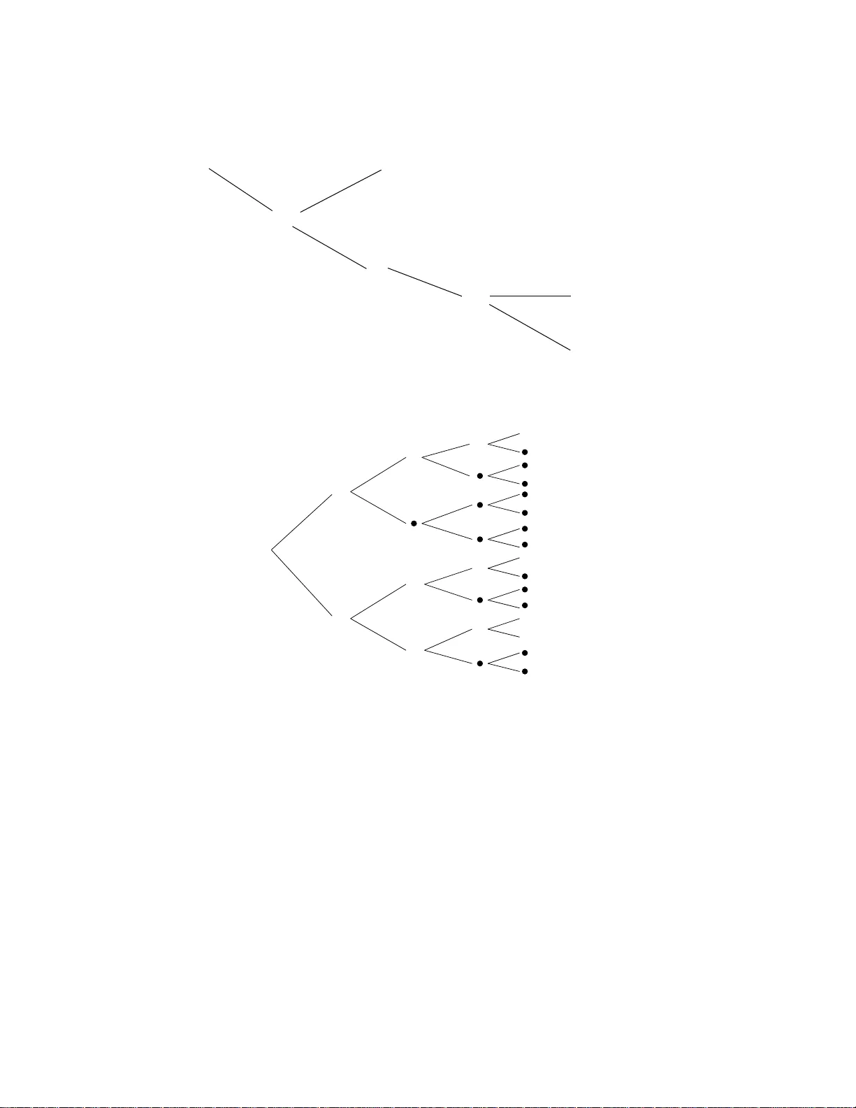
The Gaussian Man y-Help-One Distributed Source Co ding Problem Saurabha T a vil dar, Pramo d Viswanath, a nd Aaron B. W agner 19 January , 2008 Abstract Join tly Gaussian memoryless sources are ob s e rved at N distinct terminals. The goal is to efficient ly enco de the observ at ions in a distributed f a shion so as to enable reconstruction of an y one of the observ ati ons, say the fir st one, at the decod e r sub- ject to a quad r a tic fidelit y cr iterion. Our main result is a pr e cise c haracterizatio n of the rate-distortio n region when the co v ariance matrix of the sour c es satisfies a “tree- structure” condition. In this sit uation, a natural analog- digital separation sc heme optimally trades off the distributed quan tization rate tuples and the distortion in the reconstruction: eac h enco der consists of a p oint -to-p oin t Gaussian v ector quantiz er follo w ed b y a Slepian-W olf binning encod e r. W e also pr o vid e a partial con v erse that suggests that the tree structure condition is f undamen tal. 1 In tro ductio n The fo cus of this study is the problem of distributed source co ding of memoryless Gaussian sources with quadratic distortion constrain ts. The rate- distort ion region of this problem with t w o terminals has b een recen tly c haracterized [1 3]. Our fo cus, hence, is on the case when there are a t least 3 terminals. In this pap er, w e study a sp ecial case of this general problem: the so-called “many -help-one” situation depicted in Figure 1. The setup is the following: Encoder 1 Decoder R 1 x 1 R N x N Enco der N ˆ x 1 Figure 1: The many-help-one problem. 1 • Sour c es : Eac h of the N enco ders observ es a memoryless discrete-time source: enco der i observ es, ov er n discrete time instan ts, the memoryless source x n i . The observ ations across the enco ders are correlated, how ev er. Sp ecifically , the jo in t o bserv ations at time m ( x 1 ( m ) , . . . , x N ( m )) are j o in tly Gaussian. F urther, the joint observ at io ns are memoryless ov er time m . • Enc o ders : Eac h enc o der i maps the ve ctor of analog observ ations (o v er n time instan ts, sa y) into a v ector of bits (of length R i n , sa y) that is t hen comm unicated without loss to a single deco der ( o n a link with rate R i ). • De c o der : The decoder is only in terested in reconstructing one o f the sources, (sa y , x n 1 ). The fidelit y c riterion consid ered here is a quadratic one: the a v erage (o v er the statistics of the sources) l 2 distance b et w een the original source vec tor and the reconstructed v ector is required to b e no more than D n . • Pr oblem statement : The problem is to characterize t he minim um set of rates at whic h the enco ders can comm unicate with the decoder while still con v eying enough informa- tion to satisfy the quadratic distortion constrain t on the reconstruction. In this pap er, w e precisely c haracterize the rate-distortion region of a class of man y-help- one problems. A crucial step tow ards solving this problem in v olv es the introduction of a related distributed source co ding problem where the source has a “binary tree” structure; this is done in Section 2. W e show that the natural ana log-digital separation strat egy o f p oin t-to -p oint Gaussian v ector quan tization follow ed by a distributed Slepian- W olf binning sc heme is optimal for this problem (this is done in Sections 2.3 and 2.4). Next, w e sho w ho w this result can b e used to solv e v arious instances of the man y-help-one problem of in terest; this is done in Section 3. Finally , v arious ancillary a sp ects of the problem at hand are discusse d in Section 4: sp ecifically the w orst-case prop ert y of the Gaussian distribution with resp ect to the analog-digita l separation arc hitecture is demonstrated a nd a partial conv erse for the necessit y of the tree-structure condition is pro vided. 2 The Binary T ree St r u cture Problem In this section, w e tak e a short detour a w a y from the man y-help-one problem of in terest (c.f. Figure 1 ). Sp ecifically , w e in tro duce a related distributed source co ding problem that w e call the “binary tree s tructure problem”. W e s how that the natural ana lo g-digital separation arc hitecture is optimal in terms of the ra te-distortion tradeoff fo r this problem. The connec- tion b et w een t he or ig inal ma ny-help-one problem and this binary tree structure problem is made in the next section. The outline of this section is as follows: • we intro duce the source v aria bles a nd their statistical relationships first (Section 2.1); • next we specify precisely the binary tr ee structure problem (Section 2.2); 2 • we ev aluate the p erformance of the natural ana log-digital architec ture in terms of t he rate-distortion tradeoff f or the binary tree structure problem (Section 2.3); • under t he assumption that certain v ariables ha v e p ositiv e v ariance, w e deriv e a nov el outer bound to the rate-distortio n region—this inv olves a careful use of the en trop y- p ow er inequalit y (extracting critical ideas from [7, 9]) and is one of t he most importa n t tec hnical contributions of this pap er (Section 2.4); • aga in under the p ositive v ariance assumption, w e sho w t ha t the outer b ound to the rate-distortion region indeed matc hes the inner b o und deriv ed by ev aluat ing the natur a l analog-digita l separation architecture (Section 2.4); • using a contin uit y ar gumen t, we relax the p ositiv e v ariance assumption and sho w that the separation arc hitecture is optimal for a ll binary tree structure problems (Sec- tion 2.5); • finally , we sho w that Gaussian sources ar e the w orst case in the sense that a non- Gaussian source has a larger rate-distortion region than a Gaussian source with the same co v a riance matrix, so long as the Gaussian source satisfies the tree structure (Section 2.6). 2.1 Binary Gauss-Mark o v T rees Consider the Marko v binary t r ee structure of G aussian random v ariables depicted in Figure 2. F o r mally , the Gauss-Mark ov tree structure represe nts the f o llo wing Marko v c hain conditions: consider the no de denoted b y the random v ariable x ( k ) i . W e define the set of left de scendan ts, the set of right desc endan ts, and the t r ee o f x ( k ) i to b e L  x ( k ) i  =  x ( l ) j : l > k , 2 l ( i − 1) 2 k < j ≤ 2 l ( i − 0 . 5) 2 k  , R  x ( k ) i  =  x ( l ) j : l > k , 2 l ( i − 0 . 5) 2 k < j ≤ 2 l i 2 k  , T  x ( k ) i  = n x ( k ) i o ∪ R  x ( k ) i  ∪ L  x ( k ) i  , resp ectiv ely . W e define the set o f no des P  x ( k ) i  to b e: n x ( l ) j : ∀ j, l o \ T  x ( k ) i  . Then, b y definition, the Mark o v c hain condition giv en by F ig ure 2 says that conditioned on the random v ariable x ( k ) i , the sets of random v ar ia bles P  x ( k ) i  , L  x ( k ) i  , and R  x ( k ) i  are indep enden t; further, this is true fo r all pairs ( i, k ). 3 x ( L ) 2 L − 1 x (1) 1 x (2) 1 x (2) 2 x (3) 1 x (3) 2 x (3) 3 x (3) 4 x ( L − 1) 1 x ( L ) 1 x ( L ) 2 x ( L − 1) 2 L − 2 x ( L ) 2 L − 1 − 1 Figure 2: The binary t r ee structure. 2.1.1 A Specific C onst r uction No w consider the follo wing sp ecific construction of x ( k ) i s that satisfies the Mark o v c hain structure in Fig ure 2. Let m , k , and i denote the time index, the tree depth index, and t he no de within the tr ee depth index, r esp ective ly . Then define x ( k +1) 2 i − 1 ( m ) = α ( k +1) 2 i − 1 x ( k ) i ( m ) + n ( k +1) 2 i − 1 ( m ) , (1) x ( k +1) 2 i ( m ) = α ( k +1) 2 i x ( k ) i ( m ) + n ( k +1) 2 i ( m ) , (2) where the indices v ary as: m = 1 , . . . , n , (3) k = 1 , . . . , L − 1 (4) i = 1 , . . . , 2 k − 1 . (5) Here α ( k +1) 2 i − 1 and α ( k +1) 2 i are real n um b ers. The random v aria bles n n ( k ) i ( m ) , k = 2 , . . . , L, i = 1 , . . . , 2 k − 1 , m = 1 , . . . , n o (6) are independen t Gaussian random v ariables (with ze ro mean and v ariance σ 2 n ( k ) i for the index pair ( k , i ) and any m ). F urther, t hese random v a riables a r e a ll indep enden t of the ro ot 4 random v ariables n x (1) 1 ( m ) , m = 1 , . . . , n o . Finally let the ro ot random v ariables n x (1) 1 ( m ) , m = 1 , . . . , n o b e a collection of i.i.d. Ga ussian random v ariables with zero mean and v ar ia nce σ 2 x (1) 1 . F rom this construction, it readily follow s that the random v ariables satisfy the tree structure in Figure 2. F ormally: Claim 1 F or this c onstruction, the x ( k ) i satisfy the Markov chain c onditions in Figur e 2. 2.1.2 Necessit y of Construction Con v ersely , this is also the most general wa y of constructing jointly Gaussian random v ari- ables that satisfy the binary tree structure. W e state this formally b elo w: Claim 2 A ny zer o-me an, jointly Gaussian n x ( k ) i , k = 1 , . . . , L, i = 1 , . . . , 2 k − 1 o that sat- isfy the Markov tr e e structur e in Figur e 2 c an b e r epr e sente d using the ab ove c onstruction (c.f. Equations (1) and (2) ). Pro of : The s teps ar e routine: F or a fixed 1 ≤ k < L and 1 ≤ i ≤ 2 k − 1 , c onsider the Gaussian random v ariable x ( k +1) 2 i − 1 . Since it is join tly Ga ussian with all of t he v ariables in P ( x ( k +1) 2 i − 1 ), w e can write: x ( k +1) 2 i − 1 = E h x ( k +1) 2 i − 1 | P ( x ( k +1) 2 i − 1 ) i + n ( k +1) 2 i − 1 . (7) Here the random v ariable n ( k +1) 2 i − 1 is Gaussian and independen t of all the no des in P ( x ( k +1) 2 i − 1 ). F urther, the conditional expectatio n in Equation ( 7) is simply t he line ar conditional exp ec- tation that is particularly simple (this is due to the Mark o v chain conditions imp osed b y the tree structure): sp ecifically , conditioned on x ( k ) i the random v ariable of fo cus, x ( k +1) 2 i − 1 , is indep enden t of all the other v ariables in P ( x ( k +1) 2 i − 1 ). Th us we can write E h x ( k +1) 2 i − 1 | P ( x ( k +1) 2 i − 1 ) i = α ( k +1) 2 i − 1 x ( k ) i , (8) for some real num ber α ( k +1) 2 i − 1 . Substituting Equation (8) in Equation (7), w e hav e deriv ed Equation (1). The deriv a tion of Equation (2) is analogous. Since n ( k ) i is indep enden t o f P ( x ( k ) i ) for all i and k , the req uired independence conditions hold and t he conclus ion follow s. ✷ 2.2 Problem Statemen t Denote the ve ctor x (1) 1 ,n def =  x (1) 1 (1) , . . . , x (1) 1 ( n )  . (9) 5 Encoder 1 Encoder 2 Decoder R 2 L − 1 ˆ x (1) 1 x ( L ) 1 x ( L ) 2 x ( L ) 2 L − 1 Enco der 2 L − 1 R 1 R 2 Figure 3: The problem setup. Similar notation will b e used for other v ectors to be in tro duced later. Consider the follo wing distributed source co ding problem depicte d in F ig ure 3: There are 2 L − 1 distributed enco ders eac h ha ving access to a me moryless observ ation seq uence: enco der i obse rve s the memoryless random pro cess x ( L ) i,n . The goal of eac h enco der is to map the observ ation in to a discr ete set (enco der i maps its length- n observ ation into a discrete set C i ). The enco ded observ ation is then conv eye d to the cen tral decoder on ra t e-constrained links. The rate of comm unication from enco der i to the deco der is 1 n log | C i | . The deco der forms a n estimate ˆ x (1) 1 ,n of the r o ot of the bina r y tr ee, x (1) 1 ,n , based on the messages C 1 , . . . , C 2 L − 1 . The a v erage distortion of the reconstruction is 1 n n X m =1 E   x (1) 1 ( m ) − ˆ x (1) 1 ( m )  2  . The goal is to characterize the set of achie v able rates and distortions ( R 1 , · · · , R 2 L − 1 , d ), i.e., those suc h that there exists an enco der a nd deco der suc h that R i ≥ 1 n log | C i | for all i and d ≥ 1 n n X m =1 E   x (1) 1 ( m ) − ˆ x (1) 1 ( m )  2  . . W e denote the closure of this set b y RD ∗ . W e note that t w o sp ecial cases of this problem ha v e b een r esolve d in the literature: • L = 1 is the single-user Gaussian source co ding problem with quadratic distortion, • L = 2 is the Gaussian CEO problem solv ed in [7, 9]. 6 The recen t w ork in [8] studies a sp ecial case of the general tree structure depicted in Figure 2. 1 While a general outer b ound is deriv ed in [8] for that special case of the tree structure, it is sho wn to b e tigh t only fo r a certain range of the parameters in the problem (the distor t io n constrain t and the co v ar ia nce matrix of t he Gaussian sources). Our main result is t ha t a natural strategy of p oin t-to- p oint Gaussian v ector quan tization follo w ed b y Slepian-W olf binning is optimal fo r any L . In the next section w e formally presen t the natural a c hiev able strat egy and then state our main result. In the subsequen t section, w e prov e a nov el outer b ound a nd use it to establish the main result. 2.3 Analog-Digital Separation Strategy The natural ac hiev able analog -digital separation strategy is depicted in Fig ure 4: each en- co der first vector quantize s the o bserv ation as in p oin t-to- p oin t Gaussian rate distortio n theory , and then co des the quan tizer outputs using a Slepian-W olf binning sc heme. The rate VQ − 2 VQ − 1 Decoder Binning Scheme − 1 Binning Scheme − 2 Binning Scheme - 2 L − 1 x ( L ) 1 x ( L ) 2 x ( L ) 2 L − 1 V Q-2 L − 1 ˆ x (1) 1 Figure 4: The natural separation sc heme. tuples need ed b y this architecture to satisfy the distortion constraint can b e calculated b y the so-called Berger-T ung inner b o und [1]: let u def = ( u 1 , u 2 , · · · , u 2 L − 1 ) (10) denote a v ector of 2 L − 1 join tly Gaussian ra ndom v ariables. Consider the set U ( d ) of u suc h that • F or eac h i = 1 , . . . , 2 L − 1 , u i satisfies u i = α i x ( L ) i + w i , (11) where α 1 , . . . , α 2 L − 1 are constan ts and w 1 , . . . , w 2 L − 1 are indep enden t zero-mean Gaus- sian r a ndom v ariables that are als o independen t of the x ( k ) i s. It is con v enien t to ass ume that α i ∈ [0 , 1] and that w i has v ariance (1 − α 2 i ) σ 2 x ( L ) i , so that x ( L ) i and u i ha v e the same v a r ia nce. This assumption incurs no loss of generality . 1 As a n aside, we note that the material in [8] along with o ur own previous work [13] pr ovided the impetus to the pre sent work. 7 • u satisfies E   x (1) 1 − E [ x (1) 1 | u ]  2  ≤ d. (12) No w, consider A ⊆  1 , . . . , 2 L − 1  . (13) Denote the set { u i : i ∈ A} def = u A . (14) Similar notation will b e used for o t her v ectors in tro duced later. W e now hav e: Lemma 1 [Ber ger-T ung inn e r b ound [1]] The analo g-d i g ital sep ar ation ar chite ctu r e achieves c onvex hul l o f the r ate-distortion r e gion RD in def = h ( R 1 , · · · , R 2 L − 1 , d ) : ∃ u ∈ U ( d ) ∋ ∀A ⊆  1 , . . . , 2 L − 1  , X i ∈A R i ≥ I  x ( L ) A ; u A | u A c  i . (15) In p articular, RD ∗ c ontains co( RD in ) , wher e co( · ) de notes the closur e of the c onvex h ul l. The region RD in can b e explicitly computed for a giv en cov ariance matrix for the observ ed Gaussian sources. This computation is aided b y the following com binatorial structure of the set RD in . 2.3.1 Com binatorial Structure of RD in Consider a sp ecific u ∈ U ( d ) (this parameterizes a sp ecific c hoice of the analog-digita l sep a- ration arc hitecture) a nd the rate tuples ( R 1 , . . . , R 2 L − 1 ) that satisfy the conditions X i ∈A R i ≥ f ( A ) , ∀A ⊆  1 , . . . , 2 L − 1  (16) where f ( A ) def = I  x ( L ) A ; u A | u A c  . (17) Consider the follow ing prop erties of the set function f for all A 1 , A 2 ⊆  1 , . . . , 2 L − 1  . W e ha v e f ( φ ) def = 0. Lemma 2 f ( A 1 ) ≥ 0 , (18) f ( A 1 ∪ { t } ) ≥ f ( A 1 ) , ∀ t ∈  1 , . . . , 2 L − 1  , (19) f ( A 1 ∪ A 2 ) + f ( A 1 ∩ A 2 ) ≥ f ( A 1 ) + f ( A 2 ) . (20) 8 Pro of Equation (18) follo ws from the non-negativit y of mutual information. Equation (19) follo ws from t he c hain rule of mutual information: fo r t / ∈ A 1 , w e hav e f ( A 1 ∪ { t } ) = I  u A 1 ; x ( L ) t x ( L ) A 1 | u A c 1  + I  u t ; x ( L ) t x ( L ) A 1 | u ( A 1 ∪{ t } ) c  , ≥ I  u A 1 ; x ( L ) t x ( L ) A 1 | u A c 1  , = f ( A 1 ) . Finally , consider (20). Let B = { i : V ar( u i | x ( L ) i ) > 0 } . Supp ose i ∈ ( A 1 ∪ A 2 ) ∩ B c . If V ar( x ( L ) i | x ( L ) ( A 1 ∪A 2 ) c ) > 0 , then f ( A 1 ∪ A 2 ) = ∞ , so (20) trivially holds. If V ar( x ( L ) i | x ( L ) ( A 1 ∪A 2 ) c ) = 0, then V ar( x ( L ) i | x ( L ) A c 1 ) = V ar( x ( L ) i | x ( L ) A c 2 ) = V ar( x ( L ) i | x ( L ) A c 1 ∪A c 2 ) = 0 , so A 1 and A 2 can b e replaced with A 1 \{ i } and A 2 \{ i } , resp ectiv ely , without affecting the v a lidity of (20). By rep eating this pro cess a s man y times as necessary , we ma y assume that A 1 ∪ A 2 ⊂ B . This case requires the use of the Marko v prop erty satisfied b y u : in particular, we hav e b y construction u A 1 ↔ x ( L ) A 1 ↔ u A c 1 , meaning that these tree v ariables f o rm a Mark o v c hain in the sp ecified order. Th us w e can write h  u A 1 | x ( L ) A 1 , u A c 1  = X i ∈A 1 h  u i | x ( L ) i  . (21) No w w e r ewrite f ( A 1 ) as, using (21), f ( A 1 ) = h  u A 1 | u A c 1  − X i ∈A 1 h  u i | x ( L ) i  (22) = h ( u ) − h  u A c 1  − X i ∈A 1 h  u i | x ( L ) i  . (23) It follows fr o m (23) that we hav e sho wn (20) if h  u A c 1  + h  u A c 2  ≥ h  u ( A 1 ∪A 2 ) c  + h  u ( A 1 ∩A 2 ) c  , i.e., h  u A c 1 −A c 2 | u A c 1 ∩A c 2  ≥ h  u A c 1 −A c 2 | u A c 2  , whic h is true since conditioning cannot increase the differen tial entrop y . ✷ A polyhedron suc h as the one in (16) with the r ank function f satisfying the prop erties in Lemma 2 is called a c ontr a-p olymatr o id . A generic reference to the class of p olyhedrons called 9 matr oids is [15] and applications to information theory are in [11] where natural achiev a ble regions of the m ultiple access c hannel are sho wn to b e p olymatr oids a nd in [3, 14] where natural ac hiev able regions are sho wn to b e con trap olymatro ids. An imp ortant prop erty of con tra-p o lymatroids is summarized in Lemma 3.3 of [11]: the c haracterization of its v ertices. F o r π a p ermutation on the set  1 , . . . , 2 L − 1  , let b ( π ) π i def = f ( { π 1 , π 2 , . . . , π i } ) − f ( { π 1 , π 2 , . . . , π i − 1 } ) , i = 1 . . . 2 L − 1 , and b ( π ) =  b ( π ) π 1 , . . . , b ( π ) π 2 L − 1  . Then the 2 L − 1 ! p o ints  b ( π ) , π a p erm utation  , are the v er- tices of (a nd hence b elong to) t he con tra-p olymatroid (1 6). W e use this result to conclude that all of the constraints in (16) are tight for some rate tuple and there is a computationally simple w a y to find the v ertex that leads to a minimal linear functional of the ra t es [1 1]. 2.4 An ou ter b oun d for a sp ecial case W e first fo cus o n t he case in whic h σ 2 n ( k ) i > 0 for all i and k . W e a bbreviate this condition b y sa ying that “all of the noise v ariances a re p ositiv e.” T o deriv e our outer b ound, we need the follow ing definitions: • Fix 1 ≤ k ≤ L − 1 and 1 ≤ i ≤ 2 k − 1 and define the f unction f x ( k ) i ( r 1 , r 2 ) def = 1 2 log   1 + α ( k +1) 2 i − 1 σ 2 n ( k ) i σ 2 n ( k +1) 2 i − 1  1 − e − 2 r 1  + α ( k +1) 2 i σ 2 n ( k ) i σ 2 n ( k +1) 2 i  1 − e − 2 r 2    , r 1 , r 2 ≥ 0 . (24) • F or no de x ( k ) i , w e define the set of asso ciated obs e rvations to b e O  x ( k ) i  =  j : 2 L ( i − 1) 2 k < j ≤ 2 L i 2 k  . (25) • T o eac h no de in the binary tree structure of Figure 2 w e asso ciate a nonnegat ive n um b er, kno wn as noise-quantization r ate . Sp ecifically asso ciate r ( k ) i with the no de x ( k ) i . A ph ysical in terpretation fo r the nomenclature “noise quantization ra t e” will b e a v ailable during the pro of o f the outer b ound. • F or eac h no de x ( k ) i define the set r A , A c ( x ( k ) i ) to b e the set o f noise-quan tization rates (sa y , r ( l ) j ) of the v a r ia bles (sa y x ( l ) j ) in the tree of x ( k ) i whose ass o ciated o bserv ations are en tirely in A or A c and are suc h that none of the ancestors o f x ( l ) j ha v e this prop erty . F o r mally , r A , A c  x ( k ) i  = n r ( l ) j : x ( l ) j ∈ T  x ( k ) i  , O  x ( l ) j  ⊂ A or O  x ( l ) j  ⊂ A c 6 ∃ x ( b ) a ∈ T  x ( k ) i  with O  x ( b ) a  ⊂ A or O  x ( b ) a  ⊂ A c , and x ( l ) j ∈ R  x ( b ) a  ∪ L ( x ( b ) a ) o . 10 Lik ewise, we let r A ( x ( k ) i ) denote the set of noise-quantiz ation rates o f v ariables in the tree of x ( k ) i whose asso ciated observ ations ar e en tirely in A and are suc h t ha t no ne of the ancestors hav e this prop erty . F ormally , r A  x ( k ) i  = n r ( l ) j : x ( l ) j ∈ T  x ( k ) i  , O  x ( l ) j  ⊂ A 6 ∃ x ( b ) a ∈ T  x ( k ) i  with O  x ( b ) a  ⊂ A , and x ( l ) j ∈ R  x ( b ) a  ∪ L ( x ( b ) a ) o . (26) • Define the follo wing set of noise-quantiz ation rates  r ( k ) i , 1 ≤ k ≤ L, 1 ≤ i ≤ 2 k − 1  : F r ( d ) =    r ( k ) i ≥ 0 , r (1) 1 ≥ 1 2 log σ 2 x (1) 1 d , r ( k ) i ≤ f x ( k ) i  r ( k +1) 2 i − 1 , r ( k +1) 2 i     . (27) • W e ne xt implicitly defi ne a collec tion of functions of the noise-quan tization rates. Con- sider a set of noise-quan tization rates  r ( k ) i , 1 ≤ k ≤ L, 1 ≤ i ≤ 2 k − 1  in F r ( d ). Then for an y i and k , w e hav e r ( k ) i ≤ f x ( k ) i  r ( k +1) 2 i − 1 , r ( k +1) 2 i  . Since f x ( k ) i is increasing in b oth argumen ts, this implies r ( k ) i ≤ f x ( k ) i  r ( k +1) 2 i − 1 , f x ( k +1) 2 i  r ( k +2) 4 i − 1 , r ( k +2) 4 i  r ( k ) i ≤ f x ( k ) i  f x ( k +1) 2 i − 1  r ( k +2) 4 i − 3 , r ( k +2) 4 i − 2  , r ( k +1) 2 i  r ( k ) i ≤ f x ( k ) i  f x ( k +1) 2 i − 1  r ( k +2) 4 i − 3 , r ( k +2) 4 i − 2  , f x ( k +1) 2 i  r ( k +2) 4 i − 1 , r ( k +2) 4 i  . By repeating this substitution pro cess, w e ma y obtain an upper b ound on r ( k ) i in terms of the noise-quan tization rates in r A , A c  x ( k ) i  . W e implicitly define f A , A c x ( k ) i  r A , A c  x ( k ) i  (28) to b e this upp er b ound. (By con v en tion, if r A , A c ( x ( k ) i ) = { r ( k ) i } , then w e define this upp er b ound to b e r ( k ) i itself.) W e then let f A x ( k ) i  r A  x ( k ) i  11 denote the function of r A  x ( k ) i  obtained b y ev aluating the function in (28) with all of the noise quan tization rates in r A , A c  x ( k ) i  \ r A  x ( k ) i  set equal to zero. The significance of this function will b e a pparen t in the pro of of the outer b ound. • F or any set A ⊆  1 , 2 , . . . , 2 L − 1  , (29) w e define the anc estors set at level k to b e A ( k ) def = n i : O ( x ( k ) i ) ∩ A 6 = Φ o , (30) where Φ denotes the empt y set. Consider the following region, RD out , defined as RD out = n ( R 1 , · · · , R 2 L − 1 , d ) : ∃ n r ( k ) i o ∈ F r ( d ) ∋ ∀A ⊆  1 , . . . , 2 L − 1  X i ∈A R i ≥ L X k =1 X i ∈A ( k )  r ( k ) i − f A c x ( k ) i  r A c ( x ( k ) i )  o . (31) This constitutes an outer b ound to the rate-distortio n region of the binary tree structure problem: Lemma 3 F or the bi n ary tr e e structur e pr oblem in wh i c h al l of the noise varianc es ar e p ositive, RD ∗ ⊂ RD out . (32) Pro of : See App endix A. W e next sho w that the outer b ound just deriv ed matc hes the inner b ound deriv ed from the analog- digital separation arc hitecture (c.f. Lemma 1). Recall that w e use co( · ) to denote the closure of the conv ex h ull of a given set. Lemma 4 F or the bi n ary tr e e structur e pr oblem in wh i c h al l of the noise varianc es ar e p ositive, RD out = co ( RD in ) . (33) Pro of : See App endix B. 12 2.5 Main Result Using a con tin uit y argument, one can relax the a ssumption that a ll of the noise v ariables ha v e p ositive v ariance. This allo ws us to conclude our first main result of this paper: the optimalit y of the analog - digital separation arc hitecture in a c hieving the rate-distort ion region of the binary tree structure problem. Theorem 1 F or the bi n ary tr e e structur e pr oblem, the optimal r ate-distortion r e gion i s achieve d by the analo g-digital sep ar ation ar chite ctur e, RD ∗ = co ( RD in ) . Pro of See App endix C. ✷ 2.6 W orst-Case Prop ert y Up to this p o in t w e ha v e assumed tha t the source v ariables are join tly Ga ussian. In this section, we justify this a ssumption by sho wing that the rate-distortion region for other dis- tributions with t he same co v ar iance are only larg er. Let  x ( k ) i  b e a Gaussian source satisfying the tree structure a s b efore. Let  ˜ x (1) 1 , ˜ x ( L ) 1 , . . . , ˜ x ( L ) 2 L − 1  b e an alternate source with the same co v ariance of  x (1) 1 , x ( L ) 1 , . . . , x ( L ) 2 L − 1  . Note that the alternate source need not b e par t of a Mark o v tr ee. Let g RD ∗ denote the rate-distortion region of t he alternate source. The separation-based architecture yields an inner b ound on the rate-distortion region of the alternate source. Sp ecifically , let g RD in denote the region obtained b y replacing  x (1) 1 , x ( L ) 1 , . . . , x ( L ) 2 L − 1  with  ˜ x (1) 1 , ˜ x ( L ) 1 , . . . , ˜ x ( L ) 2 L − 1  in the discussion in Section 2.3. Then co  g RD in  ⊂ g RD ∗ . Theorem 2 A Gaussian sour c e satifying the binary tr e e structur e has the smal lest r a te- distortion r e gion for its c ovarianc e: RD ∗ ⊂ g RD ∗ . In fact, the sep ar ation-b ase d ar chite ctur e has the most diffi c ulty c ompr essing a Gaussia n sour c e in the sense that RD ∗ = co ( RD in ) ⊂ co  g RD in  ⊂ g RD ∗ . (34) Pro of See App endix D. ✷ 13 3 T re e Struc t ure and th e Man y-Help-One Prob l e m W e now turn to the main problem of inte rest: the man y-help-one distributed source co ding problem. As in t he tree structure problem, there is a natura l analog-digit a l separation arc hitecture that is a candidate solution. This is illustrated in Figure 5. VQ − 2 VQ − 1 Decoder Binning Scheme − 1 Binning Scheme − 2 Binning x N V Q- N ˆ x 1 Scheme - N x 2 x 1 Figure 5: The natural ana log-digital separation arc hitecture. 3.1 Main Result Our main result is a suffic ien t condition under whic h the a na log-digital separation arc hitec- ture is optimal. T o state it, w e first define a gener al Gauss-Mark o v tree: it is made up of join tly Gaussian random v a r iables and resp ects the Mark ov conditions implied b y the tree structure. The only extra feature compared to the binary Gauss-Mark o v tree (c.f. Figure 2) is that eac h no de can hav e an y n umber of descendan ts (not just tw o). Theorem 3 Consider the many-help-on e di s tribute d sour c e c o din g pr oblem il lustr ate d in Figur e 1. Supp ose the observations x 1 , . . . , x N c an b e emb e dde d in a gener al Gauss-Markov tr e e of size M ≥ N . Then the natur al an a lo g-digital sep ar ation ar chite ctur e (c.f. Figur e 5) achieves the entir e r ate-distortion r e gion . Pro of : The pro of is elemen tary and builds heavily on Theorem 1. W e o utline the steps b elo w: • A general G auss-Mark o v tree can b e recast as a (p ot en tially larger) binary G auss- Mark o v tree with the ro ot b eing identifie d with any specified no de in the original tree. T o see t his, w e only need to observ e that the Marko v c hain relations are t he same no matter whic h no de is iden tified as the ro ot. • Next, b y p oten tially increasing the height of the binary tree (to ˜ L ≥ L ) w e can ensure that the observ ations x 1 , . . . , x N are a subset of the 2 ˜ L − 1 lea v es of the binary Gauss- Mark o v tree. I f one o bserv ation of interest, say x i , is an in termediate no de o f the binary Gauss-Mark o v tree w e can effectiv ely mak e it a leaf b y adding descen dants that are iden tical (almost surely) to x i . 14 This allo ws us to con v ert the many-help-one problem in to a binary tree structure problem (with p ot entially more observ ations than we star t ed out with). The analo g-digital separation arc hitecture is optimal f or this problem (c.f. Theorem 1). By restricting the corresponding rate-distortion region to the instance when the rat es of the encoders corresp onding to the observ ations that w ere not pa rt of the original N are zero, w e still ha v e the optimality of the analog-digita l separation architecture. This latter rate-distortion regio n simply correspo nds to the man y-help-one problem studied in Fig ure 1. This completes the pro of. ✷ W e illustrate the t w o k ey steps outlined ab ov e with an example with N = 4. Supp ose that x 1 , . . . , x 4 can b e em b edded in the tree depic ted in Figure 6. This tree ha pp ens to b e binary , but unfortunately the ro ot is no t the source of interes t, x 1 . Figure 7 sho ws ho w to construct a new Gauss-Mark o v tree that still prese rve s the Mark o v conditions but has x 1 as its ro ot. Finally , a binary Gauss-Mark ov tree of heigh t 5 is constructed that has the original four observ ations as a subset of its 16 leaf no des; this is done in Figure 8 —here an y no de indicated b y a dot is simply identic ally equal (almost surely) to its paren t no de. Finally w e can set to zero the rates of all the encoders except those n um b ered 1, 9, 13 and 14. This allo ws us to capture the rate-distortion r egio n of the original thr ee-help-o ne problem. y 1 y 2 x 1 x 2 x 3 x 4 y 0 Figure 6: F our observ ations are em b edded in a (binary) Ga uss-Marko v tree. 3.2 W orst-Case Prop ert y As with our earlier result for the binary tree structure problem, the Gaussian assumption in Theorem 3 can be justified on the grounds that it is the w orst-case distribution. Sp ecifically , as in Section 2.6, let ˜ x 1 , . . . , ˜ x N denote a n alternate source with the same co v ariances a s x 1 , . . . , x N . Let g RD ∗ denote the rate-distortion region of the source, and let g RD in denote the inner b ound obtained by replacing the source v ariables in the discussion in Section 2.3 with the alternate source ˜ x 1 , . . . , ˜ x N . Theorem 4 A Gaussian so ur c e that c an b e emb e dde d in a Gauss-Markov tr e e ha s the smal l - est r ate-distortion r e gion for its c ovarianc e: RD ∗ ⊂ g RD ∗ . 15 x 2 y 1 y 0 y 2 x 3 x 4 x 1 Figure 7: The tree rewritten with x 1 as the ro ot. x 1 x 1 x 1 y 1 x 2 y 0 x 1 x 1 x 2 x 2 x 3 x 4 y 2 Figure 8: The man y-help-one problem rewritten as a binary tree structure problem. In fact, the sep ar ation-b ase d ar chite ctur e has the most diffi c ulty c ompr essing a Gaussia n sour c e in the sense that RD ∗ = co ( RD in ) ⊂ co  g RD in  ⊂ g RD ∗ . The pro o f of Theorem 2 applies verbatim here. 3.3 T ree Structure Condition and Computational V erification If N = 2, then x 1 and x 2 can alw a ys b e placed in the tr ivial Gauss-Mark o v tree consisting of these tw o v a riables; no embedding is needed in this case. W e note that N = 2 corre- sp onds to the “one-help-one” problem, whose rate-distortion region has been determined by Oohama [6 ]. With N ≥ 3, em bedding is not alw a ys possible. W e see a n e xample of this ne xt, where w e also see a simple test for when N linearly indep enden t v ariables can thems elv es b e 16 arranged in a tree, without adding additional v ariables. W e then deriv e a condition on the co v a riance matrix of x 1 , . . . , x N that is necessary for these v ariables to b e em b edded as the no des of a general Gauss-Marko v tree. Finally , w e sho w that this condition is also sufficien t when N = 3. 3.3.1 T rees Without Em b edding W e next demonstrate a simple test for when N linearly indep enden t, join tly G aussian random v a r ia bles can thems elv es b e arr a nged in a tree, without adding additional v ariables. Without loss of generalit y , we may assume that x 1 , . . . , x N eac h has unit v ariance (this c an b e ensured b y normalizing eac h observ at ion). W e shall write ρ ij = E [ x i x j ] . Supp ose that x 1 , . . . , x N are linearly indep enden t, a nd let K x denote their (in v ertible) co- v a r ia nce matrix. W e will use the follow ing fact from the literature ( Sp eed and Kiiv eri [10]): x 1 , . . . , x N are Mark ov with resp ect to a simple, undirected gra ph G if and only if for all i 6 = j suc h that ( i, j ) is not an edge in G , the ( i, j ) en try of K − 1 x is zero. No w let G denote the simple, undirected graph with x 1 , . . . , x N as the no des obtained by in terpreting K − 1 x − I as the adjacency matrix: there is an edge b et w een x i and x j if and only if the ( i, j ) elemen t o f K − 1 x − I is nonzero. It follo ws that x 1 , . . . , x N can b e arranged in a Gauss-Mark o v tree if and only if G is a tree, or more generally , a forest (i.e, a collection of unconnected trees). This fact can b e illustrated with the f o llo wing example. Supp ose that N = 3 and K x =   1 1 / 4 1 / 4 1 / 4 1 1 / 4 1 / 4 1 / 4 1   . (35) Then K − 1 x = 1 9   10 − 2 − 2 − 2 10 − 2 − 2 − 2 10   , whic h yields a f ully-connected graph. Hence x 1 , x 2 , and x 3 cannot b e arranged in a G a uss- Mark o v tr ee. Nev ertheless , it is p ossible that x 1 , x 2 , x 3 can be emb e dde d in a larger Gauss-Mark o v tree. Indeed, in this case it turns out that it is p ossible to em b ed the v a r ia bles in a t ree of size 4. W e o ffer the following sp ecific construction to demonstrate this fact. Let x 0 b e a standard Normal random v ariable and let x 1 = 1 2 · x 0 + z 1 x 2 = 1 2 · x 0 + z 2 x 3 = 1 2 · x 0 + z 3 17 where z 1 , z 2 , and z 3 are i.i.d. Gaussian with v ariance 3 / 4, and ar e independen t of x 0 . The co v a riance matrix for this quadruple of v ariables is K x =     1 1 / 2 1 / 2 1 / 2 1 / 2 1 1 / 4 1 / 4 1 / 2 1 / 4 1 1 / 4 1 / 2 1 / 4 1 / 4 1     . The in v erse of this matrix is K − 1 x = 2 3     3 − 1 − 1 − 1 − 1 2 0 0 − 1 0 2 0 − 1 0 0 2     . with the resulting G b eing the tree depicted in Fig. 9. x 1 x 0 x 3 x 2 Figure 9: T ree embedding for x 1 , x 2 , and x 3 . 3.3.2 Necessary Condition for T ree Em b edding Ev en allo wing additional v ariables in the Gauss-Mark o v tree, it can turn out that em bedding is imp ossible. T ow ards understanding the situation b etter, we deriv e a necessary condition for x 1 , . . . , x N to b e em b eddable. It turns out that this condition is also sufficien t when N = 3. Prop osition 1 L et N ≥ 3 . If x 1 , . . . , x N c an b e e m b e dde d in a Gauss-Markov tr e e, then | ρ ik | ≥ | ρ ij ρ j k | (36) and ρ ik ρ ij ρ j k ≥ 0 (37) for al l distinct i , j , and k . C onversely, if N = 3 and c onditions (36) an d (37) hold for al l distinct i j , an d k , then x 1 , . . . , x N c an b e e m b e dde d in a Gauss-Markov tr e e. Pro of See App endix E. ✷ 18 4 A P artial Con v erse W e hav e show n that if the source can b e em b edded in a G auss-Mark o v tree, then the separation-based sc heme achie v es the en tire rate-distortion r egion fo r the many-help-one problem. This raises t he question of whether the tree-em b eddability condition can b e re- laxed, or whether it is necessary in o rder for the separation-ba sed sc heme to achiev e the en tire rate-distortion region. W e next sho w that it is reasonable to conjecture that tr ee- em b eddabilit y , or a similar condition, is a necess ary and sufficien t condition for separation to ac hiev e the en tire rat e-distortion region. Our ar g umen t consists o f t w o parts. • First, we provide an ex ample t ha t show s that separation do es no t alwa ys ac hiev e the en tire rate- distort ion region for the many-help-one problem, whic h establishes that some added condition is required. • W e then establish a connection b et w een this coun terexample and the tree em b eddabil- it y condition. 4.1 Sub optimalit y of S eparation W e b egin b y sho wing that the separation-based sc heme does not alwa ys ac hiev e the en tire rate-distortion region for t he man y-help-one problem. Consider the special case of three sources ( N = 3), where x 1 and x 2 ha v e cov ariance matrix  σ 2 ρσ 2 ρσ 2 σ 2  0 < ρ < 1 . and whe re x 3 = x 1 − x 2 . W e shall assume that the goal is to reproduce x 3 at the deco der and that R 3 = 0, i.e., the help ers completely shoulder the communic ation burden. W e shall fo cus in particular on the a symptotic regime in whic h σ 2 is large and ρ is near one. Sp ecifically , let ρ = 1 − 1 2 σ 2 and consider the b eha vior of the rate-distortion regio n as σ 2 tends to infinit y . Note that the v a r ia nce o f x 3 do es not tend to infinit y , and in fa ct equals one fo r any p ositive v alue o f σ 2 , due to our ch oice of ρ . In this regime, the separation-based sc heme p erforms quite p o orly . Prop osition 2 L et 0 < d < 1 a n d let R ( σ 2 , d ) denote the minimum value of R 1 + R 2 such that ( R 1 , R 2 , 0 , d ) is in the r a te-d i s tortion r e gion for the sep ar ation-b ase d scheme. Then lim σ 2 →∞ R ( σ 2 , d ) = ∞ . Pro of Please see App endix F. ✷ W e now exhibit a sc heme whose sum rate is b ounded as σ 2 tends to infinity . This sc heme is simple in the sense that it op erates o n individual samples, not long blo c ks. Consider tw o lattices in R , Λ i = { k · 2 − n : k ∈ Z } Λ o = { k · 2 m : k ∈ Z } . 19 Let Q i ( x ) denote the lattice p oin t in Λ i that is closest t o x ; ties are brok en arbitrarily . Let x mo d Λ i = x − Q i ( x ) . Analogous definitions f or Λ o are also in effect. Let ˜ x 1 ( ℓ ) = Q i ( x 1 ( ℓ )) . F o r each time ℓ , the first enco der communic ates u 1 ( ℓ ) = ˜ x 1 ( ℓ ) mo d Λ o to the deco der. This requires sending n + m bits p er sample. The second deco der op erates analogously , yielding a sum rate o f 2( n + m ) bits p er sample. The deco der uses ˆ x 3 ( ℓ ) = [ u 1 ( ℓ ) − u 2 ( ℓ )] mod Λ o as its estimate f o r x 3 ( ℓ ). Prop osition 3 F or any d > 0 , if m and n a r e sufficiently lar ge, then E [( x 3 ( ℓ ) − ˆ x 3 ( ℓ )) 2 ] ≤ d al l ℓ and al l σ 2 . Pro of Please see App endix G. ✷ Since n and m need not tend to infinity a s σ 2 gro ws, t his simple sc heme b eats the separation-based approach by a n arbitrarily lar g e amoun t as σ 2 tends to infinity . The sc heme can b e improv ed by using higher- dimensional lattices for Λ i and Λ o . This has been explored b y Krithiv asan and Pradhan [5]. Conceptually , the difference b et w een the tw o sche mes can b e understo o d as fo llo ws. Consider the binary expansion of x 1 . The quan tity Q i ( x 1 ) mo d Λ o can b e computed from the sign of x 1 and the m bits to the left o f the binary p oint and the n + 1 bits to the righ t of the binary p oint. Thu s, Prop osition 3 sho ws that only these n + m + 2 bits are necess ary for the purp ose of repro ducing the difference x 1 − x 2 . In particular, it is not nec esssary to send the bits that a re m ore significan t than the bloc k of m to the left of the binary p oin t. As a result of using a standard v ector q uantize r, how ev er, the separation-based sc heme effectiv ely sends these most significan t bits. If t he v aria nces of x 1 and x 2 are lar ge, this is inefficien t. 20 4.2 On the Necessit y of the T ree Condition The previous section sho ws t ha t the separation-based archite cture do es no t achie v e the complete rate-distortion region w hen x 1 and x 2 are positiv ely correlated and x 3 = x 1 − x 2 , at least when the v ariances o f x 1 and x 2 are lar ge and their correlation co efficien t is near one. This is also true of the problem in which x 1 and x 2 are negativ ely cor r elated and x 3 = x 1 + x 2 . The defining feature o f these t w o examples is that if E [ x 3 | x 1 , x 2 ] = a 1 x 1 + a 2 x 2 , then a 1 · a 2 · E [ x 1 x 2 ] < 0 . (38) W e next show that f or N = 3 , if the sources cannot be embedded in a G auss-Mark o v tree, then this condition holds, except for a p ossible relab eling. Prop osition 4 F or N = 3 , if x 1 , x 2 , and x 3 c annot b e em b e dde d in a Gauss-Markov tr e e, then (38) holds for some r elab eling of x 1 , x 2 , and x 3 . Pro of Please see App endix H. ✷ A Pro o f of Lemma 3 Consider an y enco ding- deco ding pro cedure that ac hiev es the rate-distort io n tuple ( R 1 , R 2 , . . . , R 2 L − 1 , d ) for the binary tree structure problem o v er a blo ck of time of length n . Let the discrete set C i denote the output of enco der i (for i = 1 , . . . , 2 L − 1 ). W e hav e that R i ≥ 1 n log | C i | , i = 1 , . . . , 2 L − 1 (39) d ≥ 1 n n X m =1 V ar  x (1) 1 ( m ) | C  . (40) Here w e hav e denoted C def = { C 1 , . . . , C 2 L − 1 } , (41) the set of all the enco der o utputs. F urther, the distributed nature of enco ding imp oses natural Mark o v c hain conditions on the enco der outputs with resp ect to the observ ations. These Mark o v chain conditions are describ ed in Figure 10. Recall our earlier definition of the anc estors set A ( k ) (c.f. Equation (30)) A ( k ) def = n i : O ( x ( k ) i ) ∩ A 6 = Φ o , (42) where Φ is the null set. Now define x ( k ) A ,n def = n x ( k ) i,n : i ∈ A ( k ) o . (43) 21 C 1 x (1) 1 ,n x (2) 2 ,n x (2) 1 ,n x (3) 1 ,n x (3) 2 ,n x (3) 3 ,n x (3) 4 ,n x ( L − 1) 2 L − 2 ,n x ( L ) 2 L − 1 ,n x ( L − 1) 1 ,n x ( L ) 1 ,n x ( L ) 2 ,n x ( L ) 2 L − 1 − 1 ,n C 2 L − 1 − 1 C 2 L − 1 C 2 Figure 10: The tree structure with the enco der outputs ov er a blo ck of length n . Our outer b ound will consider arbitrary subsets A of  1 , . . . , 2 L − 1  . Denote the set C A def = { C i : i ∈ A} . (44) The sum of any subset A of the enco der rates satisfies n X i ∈A R i = X i ∈A log | C i | ≥ X i ∈A H ( C i ) ≥ H ( C A ) ≥ H ( C A | C A c ) = I  x ( L ) A ,n ; C A | C A c  ( a ) = I  x (1) A ,n , · · · x ( L − 1) A ,n , x ( L ) A ,n ; C A | C A c  (45) ( b ) = L X k =1 I  x ( k ) A ,n ; C A | x ( k − 1) A ,n , C A c  (46) ( c ) = L X k =1  I  x ( k ) A ,n ; C | x ( k − 1) A ,n  − I  x ( k ) A ,n ; C A c | x ( k − 1) A ,n  . (47) Here each of the steps ( a ), ( b ), and ( c ) follo w from the Mark o v c hain conditions describ ed in Fig ure 10. W e use the c hain r ule to expand each of the mutual information terms in the 22 lo w er b ound of Equation ( 4 7): I  x ( k ) A ,n ; C | x ( k − 1) A ,n  = X i ∈A ( k ) I  x ( k ) i,n ; C | x ( k − 1) A ,n , x ( k ) j,n , j < i, j ∈ A ( k )  (48) = X i ∈A ( k ) I  x ( k ) i,n ; C | x ( k − 1) ⌊ i +1 2 ⌋ ,n  , (49) and I  x ( k ) A ,n ; C A c | x ( k − 1) A ,n  = X i ∈A ( k ) I  x ( k ) i,n ; C A c | x ( k − 1) A ,n , x ( k ) j,n , j < i, j ∈ A ( k )  (50) = X i ∈A ( k ) I  x ( k ) i,n ; C A c | x ( k − 1) ⌊ i +1 2 ⌋ ,n  (51) Here b oth Equations (49) and (51) follow from the Mark o v chain conditions described in Figure 10. D enote b y r ( k ) i def = 1 n I  x ( k ) i,n ; C | x ( k − 1) ⌊ i +1 2 ⌋ ,n  , (52) the term inside the summation in Equation (4 9). Then r (1) 1 is the num ber of bits per sample that the enco ders send abo ut the ro ot o f the tree and r ( k ) i for k > 1 can b e in terpreted as the num ber of bits p er sample that the enco ders use to represen t the no ise in tro duced a t no de x ( k ) i . W e will upp er b ound the terms inside the summation in Equation (51) in terms of these quan tities. T o do this, w e start with a cen tral preliminary lemma. A.1 A Preliminary Lemma Consider four memoryless join tly Gaussian random pro cesses w ( m ) , x ( m ) , y ( m ) , z ( m ) , m = 1 , . . . , n . They are iden tically join tly distributed in the (time) index m . A t any given time index m , their jo in t distribution satisfies the Mark ov c hain conditions implied in Figure 11. Then w e can write, for all m = 1 , . . . , n , x w y z Figure 11: The Marko v c hain conditio ns. x ( m ) = α xw w ( m ) + n 0 ( m ) , y ( m ) = α y x x ( m ) + n 1 ( m ) , z ( m ) = α z x x ( m ) + n 2 ( m ) , 23 for some real α xw , α y x , α z x . Here n 0 ( m ) , n 1 ( m ) , n 2 ( m ) , m = 1 . . . , n , are i.i.d. in time and indep enden t of each other and indep enden t of the pro cess w ( m ) , m = 1 , . . . , n . F urther, the random v a riables n 0 ( m ) , n 1 ( m ) , n 2 ( m ) , w ( m ) at an y time index n are N (0 , σ 2 n 0 ) , N (0 , σ 2 n 1 ) , N (0 , σ 2 n 2 ), and N (0 , σ 2 w ) resp ective ly . W rite t he v ectors w n = [ w (1) , . . . , w ( n )] (53) x n = [ x (1) , . . . , x ( n )] (54 ) y n = [ y (1 ) , . . . , y ( n )] ( 5 5) z n = [ z (1) , . . . , z ( n )] . (56) Consider t w o random v ariables C 1 , C 2 that satisfy t he following tw o Mark o v chain conditions: ( w n , x n , z n , C 2 ) ↔ y n ↔ C 1 , (57) ( w n , x n , y n , C 1 ) ↔ z n ↔ C 2 , (58) Our first inequalit y concerns this Mark o v c hain condition. W e in ten tionally use notation similar to that intro duced in Section 2.4 . Lemma 5 Define r 1 def = 1 n I ( y n ; C 1 | x n ) , r 2 def = 1 n I ( z n ; C 2 | x n ) , f x ( r 1 , r 2 ) def = 1 2 log  1 + α 2 y x σ 2 n 0 σ 2 n 1  1 − e − 2 r 1  + α 2 z x σ 2 n 0 σ 2 n 2  1 − e − 2 r 2   . Then 1 n I ( x n ; C 1 , C 2 | w n ) ≤ f x ( r 1 , r 2 ) , (59) 1 n I ( x n ; C 1 | w n ) ≤ f x ( r 1 , 0) , (60 ) 1 n I ( x n ; C 2 | w n ) ≤ f x (0 , r 2 ) . (61) Pro of : This lemma is a conditional ve rsion (conditioned on w n ) of Lemma 3 in [7]. Th e pro of follow s “mutatis mutandis” that of Lemma 3 in [7]; the only extra fact nee ded is that conditioned o n any realization of w n , ( x n , y n , z n ) are join tly Gaussian with their original v a r ia nces and ( x n , y n , z n , C 1 , C 2 ) satisfies the Mark o v condition C 1 ↔ y n ↔ x n ↔ z n ↔ C 2 . Sp ecifically , supp ose first that α y x and α z x are nonzero. F or any realization of w n , sa y ˜ w n , Oohama [7, Lemma 3 ] has sho wn that 1 n I ( x n ; C 1 , C 2 | w n = ˜ w n ) ≤ f x ( r 1 , r 2 ) . 24 By av eraging the left-hand side o v er ˜ w n , w e obta in (59). The pro ofs o f (60) and (61) are similar. If bot h α y x and α z x are zero, then the result is tr ivial. If, sa y , only α y x is zero, then I ( x n ; C 1 , C 2 | w n ) = I ( x n ; C 2 | w n ) and (59) follows from (61). ✷ A.1.1 Sufficien t Conditions for E qualit y It is useful to o bserv e the conditions for equalit y in ( 5 9), (60) and (61): supp ose C k = [ u k (1) , . . . , u k ( n )] , k = 1 , 2 . (62) Here u 1 ( m ) = α 1 y ( m ) + v 1 ( m ) , m = 1 , · · · , n, u 2 ( m ) = α 2 z ( m ) + v 2 ( m ) , m = 1 , · · · , n, where v 1 ( m ) and v 2 ( m ) are Ga ussian and indep endent of e ach other and of w n , x n , y n , z n and are i.i.d. in t he time index m . Then it is verifie d directly that with this c hoice of C 1 , C 2 (c.f. Equation (62)) the inequalities in Equations (59 ), ( 6 0) and (61 ) are all sim ultaneously met with equality (this v erification is also done in [7 , 9]). This fact will b e us ed later to sho w that the ac hiev a ble region of the separation-based inner b ound coincides with the outer b ound. A.1.2 An Impor tan t Instance Of sp ecific in terest to us will b e the following asso ciation of the random v ariables in Figure 11 to the binary tree structure in Figure 2: fix 1 ≤ k ≤ L − 1 and 1 ≤ i ≤ 2 k − 1 . Then let x = x ( k ) i (63) y = x ( k +1) 2 i − 1 (64) z = x ( k +1) 2 i (65) w = x ( k − 1) ⌊ i +1 2 ⌋ . (66) With this asso ciation, denote the function cor r esp o nding to f x in Equation (59) by f x ( k ) i : f x ( k ) i ( r 1 , r 2 ) def = 1 2 log   1 + α ( k +1) 2 i − 1 σ 2 n ( k ) i σ 2 n ( k +1) 2 i − 1  1 − e − 2 r 1  + α ( k +1) 2 i σ 2 n ( k ) i σ 2 n ( k +1) 2 i  1 − e − 2 r 2    , r 1 , r 2 ≥ 0 . (67) Indeed, this is the same notation as that introduced in Section 2.4 (c.f. Equation (24)). A.2 An Iteration Lemma As an immediate application of the preliminary lemma derived in the previous section, consider an y subset A ⊆  1 , . . . , 2 L − 1  . Fix 1 ≤ k ≤ L − 1 and 1 ≤ i ≤ 2 k − 1 . F or simplic ity of notation, let us supp ose that x (0) 1 is a zero random v ariable. 25 Lemma 6 1 n I  x ( k ) i,n ; C A | x ( k − 1) ⌊ i +1 2 ⌋ ,n  ≤ f x ( k ) i  1 n I  x ( k +1) 2 i − 1 ,n ; C A | x ( k ) i,n  , 1 n I  x ( k +1) 2 i,n ; C A | x ( k ) i,n   . (68) Pro of : F or any no de x ( k ) i , recall the set of asso ciated obs e rvations defined as (c.f. Equa- tion (25)) O  x ( k ) i  =  j : 2 L ( i − 1) 2 k < j ≤ 2 L i 2 k  . With this definition, w e observ e that O  x ( k ) i  = O  x ( k +1) 2 i − 1  ∪ O  x ( k +1) 2 i  , I  x ( k ) i,n ; C A | x ( k − 1) ⌊ i +1 2 ⌋ ,n  = I  x ( k ) i,n ; C A∩O “ x ( k ) i ” | x ( k − 1) ⌊ i +1 2 ⌋ ,n  . Then w e only need to in v ok e Lemma 5 with the follo wing random v ariables: w n = x ( k − 1) ⌊ i +1 2 ⌋ ,n , x n = x ( k ) i,n , y n = x ( k +1) 2 i − 1 ,n , z n = x ( k +1) 2 i,n , C 1 = C A∩O “ x ( k +1) 2 i − 1 ” , C 2 = C A∩O “ x ( k +1) 2 i ” . This completes the pro of. ✷ Observ e that the parameters inside the function f x ( k ) i ( · , · ) are themselv es of t he t yp e of the term in the left hand side of Equation (68). Then, w e can r ep eatedly apply Lemma 6. As a n example, we ha v e for k ≤ L − 2 and 1 ≤ i ≤ 2 k − 1 , the tw o para meters of f x ( k ) i in Equation (68) are upp er b ounded by 1 n I  x ( k +1) 2 i − 1 ,n ; C A | x ( k ) i,n  ≤ f x ( k +1) 2 i − 1  1 n I  x ( k +2) 4 i − 3 ,n ; C A | x ( k +1) 2 i − 1 ,n  , 1 n I  x ( k +2) 4 i − 2 ,n ; C A | x ( k +1) 2 i − 1 ,n   . (69) 1 n I  x ( k +1) 2 i,n ; C A | x ( k ) i,n  ≤ f x ( k +1) 2 i  1 n I  x ( k +2) 4 i − 1 ,n ; C A | x ( k +1) 2 i,n  , 1 n I  x ( k +2) 4 i,n ; C A | x ( k +1) 2 i,n   . (70) No w the function f x ( k ) i ( · , · ) is monotonically increasing in b ot h of its parameters (this is true for eac h 1 ≤ k ≤ L − 1 and 1 ≤ i ≤ 2 k − 1 ). So, we can com bine Equations (68), (7 0) and (69) to get 1 n I ( x ( k ) i,n ; C A | x ( k − 1) ⌊ i +1 2 ⌋ ,n ) ≤ f x ( k ) i  f x ( k +1) 2 i − 1  1 n I  x ( k +2) 4 i − 3 ,n ; C A | x ( k +1) 2 i − 1 ,n  , 1 n I  x ( k +2) 4 i − 2 ,n ; C A | x ( k +1) 2 i − 1 ,n   , f x ( k +1) 2 i  1 n I  x ( k +2) 4 i − 1 ,n ; C A | x ( k +1) 2 i,n  , 1 n I  x ( k +2) 4 i,n ; C A | x ( k +1) 2 i,n   . (71 ) 26 The stage is no w set to recursiv ely apply L emma 6. Contin uing this pro cess until the b oundary conditions are met, w e arr ive at 1 n I  x ( k ) i,n ; C A | x ( k − 1) ⌊ i +1 2 ⌋ ,n  ≤ f A x ( k ) i  r A  x ( k ) i  . (72) Here the set r A  x ( k ) i  is defined as in Equation (26): r A  x ( k ) i  = n r ( l ) j : x ( l ) j ∈ T  x ( k ) i  , O ( x ( l ) j ) ⊂ A , 6 ∃ x ( b ) a ∈ T  x ( k ) i  with O  x ( b ) a  ⊂ A , and x ( l ) j ∈ R  x ( b ) a  ∪ L ( x ( b ) a ) o . (73) The function f A x ( k ) i ( · ) w as also defined in Section 2.4. A.3 Putting Them T ogether W e are now ready to complete the pro of of Lemma 3. First, w e substitute Equation (72) in Equation (51) to get I  x ( k ) A ,n ; C A c | x ( k − 1) A ,n  ≤ X i ∈A ( k ) f A c x ( k ) i  r A c  x ( k ) i  . (74) Com bining Equation (74) with Equations (49) and (52), w e can rewrite the inequalit y in Equation (47) as X i ∈A R i ≥ L X k =1 X i ∈A ( k )  r ( k ) i − f A c x ( k ) i  r A c ( x ( k ) i )  . (75) The quan tities r ( k ) i satisfy other natural inequalities as w ell: • Supp o sing that A equals the en tire set  1 , 2 , . . . , 2 L − 1  and substituting in Lemma 6 w e ha v e r ( k ) i ≤ f ( k +1) x i  r ( k +1) 2 i − 1 , r ( k +1) 2 i  . (76) 27 • By direct calculatio n w e also ha v e r (1) 1 = 1 n I  x (1) 1 ,n ; C  (77) = 1 n h  x (1) 1 ,n  − 1 n h  x (1) 1 ,n | C  (78) ≥ 1 2 log  2 π eσ 2 x (1) 1  − 1 n h  x (1) 1 ,n − E h x (1) 1 ,n | C i (79) ≥ 1 2 log  σ 2 x (1) 1  − 1 2 n log det  Co v a r  x (1) 1 ,n − E h x (1) 1 ,n | C i (80) ≥ 1 2 log  σ 2 x (1) 1  − 1 2 log  1 n T race  Co v a r  x (1) 1 ,n − E h x (1) 1 ,n | C i  (81) = 1 2 log  σ 2 x (1) 1  − 1 2 log 1 n n X m =1 V ar  x (1) 1 ( m ) | C  ! (82) ≥ 1 2 log σ 2 x (1) 1 d . (83) where: – Equation (79) follo ws from the fact that conditioning only reduces the differen tial en trop y; – Equation (80 ) is the usual b ound on the differential en trop y of a vec tor by the determinan t of its co v ariance matrix; – Equation (81 ) follows fr om the Hada mard inequalit y on the determinan t of a p ositiv e definite matrix in terms of its trace; – Equation (83) follo ws from the fact that the enco der outputs describ e the original ro ot no de of the tree with sufficien tly small quadratic fidelit y (c.f. Eq uation (4 0)). Based on Equations ( 7 6) and (83) w e see that the set of r ( k ) i indeed b elong to the set F r ( d ) defined in Equation (27). Com bining this fact with the k ey inequalit y in Equation ( 7 5), w e ha v e completed the pro of of the outer b ound in Lemma 3 . ✷ B Pro of o f Lemma 4 Since w e kno w that co( RD in ) ⊂ RD out , (84) it s uffices to pro v e that for an y d and an y c omp o nen t wise nonnegativ e v ector ( α 1 , . . . , α 2 L − 1 ), inf R :( R ,d ) ∈RD out 2 L − 1 X i =1 α i R i ≥ inf R :( R ,d ) ∈RD in 2 L − 1 X i =1 α i R i . 28 W e will assume that α 1 ≤ α 2 ≤ · · · ≤ α 2 L − 1 . The pro of for the other orderings is similar. W e will a lso use the con v en tion α 0 = 0. No w for any R 1 , . . . , R 2 L − 1 , 2 L − 1 X i =1 α i R i = α 1 2 L − 1 X i =1 R i + ( α 2 − α 1 ) 2 L − 1 X i =2 R i + · · · + ( α 2 L − 1 − α 2 L − 1 − 1 ) R 2 L − 1 , = 2 L − 1 X j =1 ( α j − α j − 1 ) 2 L − 1 X i = j R i Th us inf R :( R ,d ) ∈RD out 2 L − 1 X i =1 α i R i = inf R :( R ,d ) ∈RD out 2 L − 1 X j =1 ( α j − α j − 1 ) 2 L − 1 X i =1 R i . Let ǫ > 0 . Then there exists s ∈ F r ( d ) and R ∗ suc h that 2 L − 1 X j =1 ( α j − α j − 1 ) 2 L − 1 X i =1 R ∗ i ≤ inf R :( R ,d ) ∈RD out 2 L − 1 X j =1 ( α j − α j − 1 ) 2 L − 1 X i =1 R i + ǫ and X i ∈A R ∗ i ≥ L X k =1 X i ∈A ( k )  s ( k ) i − f A c x ( k ) i ( s A c ( x ( k ) i ))  for all A . Let A j = { j, . . . , 2 L − 1 } ∩ { i : s ( L ) i > 0 } . Then 2 L − 1 X j =1 ( α j − α j − 1 ) 2 L − 1 X i =1 R ∗ i ≥ 2 L − 1 X j =1 ( α j − α j − 1 ) X i ∈A j R ∗ i ≥ 2 L − 1 X j =1 ( α j − α j − 1 ) L X k =1 X i ∈A ( k ) j ( s ( k ) i − f A c j x ( k ) i ( s A c ( x ( k ) i ))) ≥ inf 2 L − 1 X j =1 ( α j − α j − 1 ) L X k =1 X i ∈A ( k ) j ( r ( k ) i − f A c j x ( k ) i ( r A c ( x ( k ) i ))) , 29 where the infim um is ov er all r in F r ( d ) suc h that r ( L ) i = 0 if and only if s ( L ) i = 0. Then there exists ˜ s ∈ F r ( d ) suc h that ˜ s ( L ) i = 0 if and only if s ( L ) i = 0 and 2 L − 1 X j =1 ( α j − α j − 1 ) L X k =1 X i ∈A ( k ) j ( ˜ s ( k ) i − f A c j x ( k ) i ( ˜ s A c ( x ( k ) i ))) ≤ inf 2 L − 1 X j =1 ( α j − α j − 1 ) L X k =1 X i ∈A ( k ) j ( r ( k ) i − f A c j x ( k ) i ( r A c j ( x ( k ) i ))) + ǫ (85) and the ˜ s minimize L X k =1 2 k − 1 X i =1 ˜ s ( k ) i . (86) No w since the ˜ s ( k ) i are in F r ( d ), w e hav e ˜ s (1) 1 ≥ 1 2 log σ 2 x (1) 1 d (87) ˜ s ( k ) i ≤ f x ( k ) i ( s ( k +1) 2 i − 1 , s ( k +1) 2 i ) . (88) W e will show that bo th of these inequalities m ust a ctually b e equalities . Since the left-hand side of (85) is monotonically decreasing in s (1) 1 and the s ( k ) i minimize (86), it follo ws that the s (1) 1 inequalit y mu st b e tight. Next supp ose that ˜ s ( n ) m < f x ( n ) m ( ˜ s ( n +1) 2 m − 1 , ˜ s ( n +1) 2 m ) (89) for some non-leaf node x ( n ) m . W e will show that this is inc ompatible with the assumption that the ˜ s ( k ) i minimize (86). Without loss of generalit y , w e may assume that none of the c hildren of x ( n ) m ha v e a strict inequalit y in (8 8). In o rder for (89) to hold, ˜ s ( L ) j m ust b e p ositiv e for at least one leaf v ariable x ( L ) j under x ( n ) m . Consider the leaf v ariable x ( L ) ˆ m under x ( n ) m with the largest index ˆ m suc h that ˜ s ( L ) ˆ m is p o sitiv e: ˆ m = arg max  2 L ( m − 1) 2 n < j ≤ 2 L m 2 n : ˜ s ( L ) j > 0  . Then consider the descendan t of x ( n ) m , x ( n +1) ˜ m , that leads to the leaf v a r ia ble x ( L ) ˆ m . Note that w e mus t hav e ˜ s ( n +1) ˜ m > 0. Supp ose that w e decrease ˜ s ( n +1) ˜ m b y a sligh t amoun t suc h tha t (8 9) still holds. F ix a j in { 1 , . . . , 2 L − 1 } and consider the sum L X k =1 X i ∈A ( k ) j  ˜ s ( k ) i − f A c j x ( k ) i  ˜ s A c j ( x ( k ) i )   , (90) 30 and recall that A j = { j, . . . , 2 L − 1 } ∩ { i : ˜ s L i > 0 } . No w if j > ˆ m , then a ll of the observ ations under x ( n ) m are in A c j , whic h implies that the sum in (90) do es not dep end on ˜ s ( n +1) ˜ m . On the other hand, if j ≤ ˆ m , then no t all of the observ ations under ˜ s ( n +1) ˜ m are in A c j , and so ˜ s ( n +1) ˜ m / ∈ ˜ s A c j  x ( k ) i  for all x ( k ) i . It fo llows that t he ob jectiv e in (85) is not increased while the sum in (86) is reduced by decreasing ˜ s ( n +1) ˜ m , w hic h is a contradiction. Th us (89) cannot hold at an y non-leaf no des in the tr ee. W e hav e th us show n tha t equalit y mus t hold in (87) and (88). W e ar e no w in a p o sition to sho w that 2 L − 1 X j =1 ( α j − α j − 1 ) L X k =1 X i ∈A ( k ) j ( ˜ s ( k ) i − f A c j x ( k ) i ( ˜ s A c j ( x ( k ) i ))) ≥ inf R :( R ,d ) ∈RD in ( d ) 2 L − 1 X i =1 α i R i . Sp ecifically , choose the auxiliary random v ariables u in the Berger-T ung inner b ound suc h that I ( x ( L ) i ; u i | x ( L − 1) ⌊ i +1 2 ⌋ ) = ˜ s ( L ) i for eac h o bserv ation i . W e will first show by induction that I ( x ( k ) i ; u | x ( k − 1) ⌊ ( i +1) / 2 ⌋ ) = ˜ s ( k ) i (91) for all v ariables x ( k ) i in the tr ee. This is true of the leaf v ariables x ( L ) i , i = 1 , . . . , 2 L − 1 b y h yp othesis. Next consider a v ariable x ( k ) i and supp ose the condition holds fo r x ( k +1) 2 i − 1 and x ( k +1) 2 i . By the o bserv ation in App endix A.1.1 , I ( x ( k ) i ; u | x ( k − 1) ⌊ ( i +1) / 2 ⌋ ) = f x ( k ) i ( I ( x ( k +1) 2 i − 1 ; u | x ( k ) i ) , I ( x ( k +1) 2 i ; u | x ( k ) i )) = f x ( k ) i ( ˜ s ( k +1) 2 i − 1 , ˜ s ( k +1) 2 i ) = ˜ s ( k ) i . This establishes (91). Then E [( x (1) 1 − E [ x (1) 1 | u ]) 2 ] = σ 2 x (1) 1 exp( − 2 ˜ s (1) 1 ) = d . Th us u is in U ( d ). If we let ˜ R i = I ( x ( L ) i ; u i | u 1 , . . . , u i − 1 ) , 31 then ( ˜ R , d ) is in RD in . Since u i is conditionally indep enden t of u and all of the source v a r ia bles giv en x ( L ) i , it follow s that ˜ s ( L ) i = 0 if and only if u i is indep endent of all of the other v a r ia bles. W e will sho w that 2 L − 1 X i = j ˜ R i = I ( x ( L ) j , . . . , x ( L ) 2 L − 1 ; u j , . . . , u 2 L − 1 | u 1 , . . . , u j − 1 ) b y induction. F or j = 2 L − 1 , this condition holds b y t he definition of ˜ R j . Next supp ose that the condition holds for j . Then b y the tree structure, 2 L − 1 X i = j − 1 ˜ R i = I ( x ( L ) j − 1 ; u j − 1 | u 1 , . . . , u j − 2 ) + I ( x ( L ) j , . . . , x ( L ) 2 L − 1 ; u j , . . . , u 2 L − 1 | u 1 , . . . , u j − 1 ) = I ( x ( L ) j − 1 , . . . , x ( L ) 2 L − 1 ; u j − 1 | u 1 , . . . , u j − 2 ) + I ( x ( L ) j − 1 , . . . , x ( L ) 2 L − 1 ; u j , . . . , u 2 L − 1 | u 1 , . . . , u j − 1 ) = I ( x ( L ) j − 1 , . . . , x ( L ) 2 L − 1 ; u j − 1 , . . . , u 2 L − 1 | u 1 , . . . , u j − 2 ) . Th us inf R :( R ,d ) ∈RD in ( d ) 2 L − 1 X i =1 α i R i ≤ 2 L − 1 X i =1 α i ˜ R i ≤ 2 L − 1 X j =1 ( α j − α j − 1 ) I ( x ( L ) j , . . . , x ( L ) 2 L − 1 ; u j , . . . , u 2 L − 1 | u 1 , . . . , u j − 1 ) = 2 L − 1 X j =1 ( α j − α j − 1 ) I ( x ( L ) A j ; u A j | u A c j ) . By mimic king (45) through (51), one can sho w that I ( x ( L ) A j ; u A j | u A c j ) = L X k =1 X i ∈A ( k ) j ( ˜ s ( k ) i − I ( x ( k ) i ; u A c j | x ( k − 1) ⌊ ( i +1) / 2 ⌋ )) . But b y Lemma 6 and the observ atio n in App endix A.1.1, I ( x ( k ) i ; u A c j | x ( k − 1) ⌊ ( i +1) / 2 ⌋ ) = f A c j x ( k ) i ( ˜ s A c j ( x ( k ) i )) . It follows tha t inf R :( R ,d ) ∈RD in 2 L − 1 X i =1 α i R i ≤ inf R :( R ,d ) ∈RD out 2 L − 1 X i =1 α i R i + 2 ǫ. Since ǫ w as arbit r a ry , the pro of is complete. 32 C Pro of o f Theo rem 1 W e m ust sho w that RD ∗ ⊆ co( RD in ). Since b o th sets are conv ex, it suffices to sho w that for an y comp onent wise nonnegative v ector ( β 1 , . . . , β 2 L − 1 , β ) inf ( R ,d ) ∈RD ∗ 2 L − 1 X i =1 β i R i + β d ≥ inf ( R ,d ) ∈ co( RD in ) 2 L − 1 X i =1 β i R i + β d (92) = inf ( R ,d ) ∈RD in 2 L − 1 X i =1 β i R i + β d . W e shall assume t hat β 1 ≤ β 2 ≤ · · · ≤ β 2 L − 1 ; the other cases are similar. Let us temp orar ily use RD ∗ ( K x ) to de note the ra t e-distortion regio n for the binary tree structure problem when the source v aria bles ha v e co v aria nce matrix K x and similarly for RD in ( K x ). If K x is suc h that all of the noise v ariances are p ositive , then (92) f ollo ws from Lemma 3. If some of the noise v ariances are zero, then let K ( n ) x b e a sequence of source co v ariance matrices con v erging t o K x suc h that for each n , K ( n ) x corresp onds to a source satisfying the binary tree structure f or whic h all of the noise v ariances are p o sitive. Then RD ∗ ( K ( n ) x ) = co( RD in ( K ( n ) x )) for eac h n , so inf ( R ,d ) ∈RD ∗ ( K ( n ) x ) 2 L − 1 X i =1 β i R i + β d = inf ( R ,d ) ∈RD in ( K ( n ) x ) 2 L − 1 X i =1 β i R i + β d . W e will first sho w that lim inf n →∞ inf ( R ,d ) ∈RD in ( K ( n ) x ) 2 L − 1 X i =1 β i R i + β d ≥ inf ( R ,d ) ∈RD in ( K x ) 2 L − 1 X i =1 β i R i + β d . (93) F o r each n , there exists a set of auxiliary random v ariables u ( n ) suc h t hat [11, Lemma 3.3] inf ( R ,d ) ∈RD in ( K ( n ) x ) 2 L − 1 X i =1 β i R i + β d = 2 L − 1 X i =1 β i I ( u ( n ) i ; x ( L,n ) i | x ( L,n ) 1 , . . . , x ( L,n ) i − 1 ) + β E   x (1 ,n ) 1 − E [ x (1 ,n ) 1 | u ( n ) ]  2  . (94) Here x ( L,n ) i denotes the i th v ariable at depth L of the tree corresp onding to co v aria nce matrix K ( n ) x . No w the auxiliary random v ariables u ( n ) can b e parametrized by a compact set, so consider a subse quence of K ( n ) x along whic h u ( n ) con v erges in distribution t o a limit u and 33 the righ t-hand side of (94) con v erges to the lim inf . Then lim inf n →∞ inf ( R ,d ) ∈RD in ( K ( n ) x ) 2 L − 1 X i =1 β i R i + β d = 2 L − 1 X i =1 β i I ( u i ; x ( L ) i | x ( L ) 1 , . . . , x ( L ) i − 1 ) + β E   ( x (1) 1 − E [ x (1) 1 | u ]  2  ≥ inf ( R ,d ) ∈RD in ( K x ) 2 L − 1 X i =1 β i R i + β d . This establishes (93). On the other hand, Chen and W agner [2] ha v e shown that the rate- distortion region is inner-semicon tin uous: lim sup n →∞ inf ( R ,d ) ∈RD ∗ ( K ( n ) x ) 2 L − 1 X i =1 β i R i + β d ≤ inf ( R ,d ) ∈RD ∗ ( K x ) 2 L − 1 X i =1 β i R i + β d . T ogether with (93), this establishes (92) and hence Theorem 1. D Pro of o f Theor e m 2 It suffices to sho w (34). If ( R , d ) is in RD in , then there exist auxiliary random v ariables u in U ( d ) suc h that d ≥ E   x (1) 1 − E [ x (1) 1 | u ]  2  and X i ∈A R i ≥ I  x ( L ) A ; u A | u A c  for all A . No w for eac h i , u i = α i x ( L ) i + w i , where w i is G a ussian and indep enden t of x ( L ) i . Let ˜ u i b e a quan tized v ersion of ˜ x ( L ) i using the same test channel ˜ u i = α i ˜ x ( L ) i + w i . Let MMSE  x (1) 1 | u  denote t he mean-square error of the minim um mean-square error (MMSE) estimate of x (1) 1 giv en u . Lik ewise, let LLSE  x (1) 1 | u  denote the mean-square error 34 of the linear least-square error (LLSE) estimate of x (1) 1 giv en u . Then E   ˜ x (1) 1 − E [ ˜ x (1) 1 | ˜ u ]  2  = MM SE ( ˜ x (1) 1 | ˜ u ) ≤ LLSE( ˜ x (1) 1 | ˜ u ) = LLSE( x (1) 1 | u ) = MM SE ( x (1) 1 | u ) ≤ d. Also, for any A , X i ∈ A R i ≥ I ( x ( L ) A ; u A | u A c ) = h ( u A | u A c ) − h ( u A | u A c , x ( L ) A ) = h ( u A | u A c ) − h ( u A | x ( L ) A ) ≥ h ( ˜ u A | ˜ u A c ) − h ( u A | x ( L ) A ) = h ( ˜ u A | ˜ u A c ) − h ( ˜ u A | ˜ x ( L ) A ) = h ( ˜ u A | ˜ u A c ) − h ( ˜ u A | ˜ u A c , ˜ x ( L ) A ) = I ( ˜ x ( L ) A ; ˜ u A | ˜ u A c ) where in the inequality w e hav e used the fact that the G aussian distribution maximizes en trop y f or a fixed co v ariance. It follows t hat ( R , d ) is in g RD in . E Pro o f of Prop os i tion 1 Supp ose that x 1 , . . . , x N can b e embedded in a Gauss-Mark ov tree a nd fix distinct indices i , j , and k . Without lo ss of generality , we ma y assume that all v aria bles in the tree ha v e mean zero and v ariance one. Consider tw o paths (i.e., t w o sequences of v ariables), one fro m x i to x j and one from x i to x k . Eviden tly b oth paths contain x i ; let x denote the last v ariable in the first pat h that is con tained in the second. This is t he p oint at whic h the t w o paths split, as sho wn in Fig. 12. Note that it is p ossible for x to equal x i , x j , or x k . No w since x is a lo ng the path from x i to x j , it follo ws from the tree condition that x i ↔ x ↔ x j . Lik ewise x i ↔ x ↔ x k . Since all of the v ar ia bles are standard Normals, this implies [16, (5.13)] ρ ij = E [ x i x ] E [ xx j ] (95) ρ ik = E [ x i x ] E [ xx k ] . (96) Next consider the paths from x j to x i and from x j to x k , and let ˜ x denote the last v ar ia ble in the first path that is con tained in the second. Then b oth x and ˜ x lie along the pat h from 35 x i x k · · · x . . . · · · x j Figure 12: x is the p oin t a t which the t w o paths split. x j to x i . If x 6 = ˜ x , then the path fr om x to x k to ˜ x to x would form a lo o p, whic h is imp o ssible since the graph is a tree. Th us ˜ x must equal x . Th us x j ↔ x ↔ x k and ρ j k = E [ x j x ] E [ xx k ] . Com bining this equation with (95) and (96 ) yields conditions (36 ) and (37). No w suppose that N = 3 and c onditions (36) and (37) hold. If ρ ij is nonzero for all i 6 = j , then 0 < ρ ij ρ ik ρ j k ≤ 1 for all distinct i , j , and k . This implies that x 1 , x 2 , and x 3 , can b e written x 1 = r ρ 12 ρ 13 ρ 23 · sgn( ρ 23 ) · x 0 + z 1 x 2 = r ρ 12 ρ 23 ρ 13 · sgn( ρ 13 ) · x 0 + z 2 x 3 = r ρ 13 ρ 23 ρ 12 · sgn( ρ 12 ) · x 0 + z 3 , where sgn( · ) is the signum function sgn( ρ ) =      1 if ρ > 0 0 if ρ = 0 − 1 if ρ < 0 , and where x 0 , z 1 , z 2 , z 3 are indep enden t Ga ussian random v ariables. Here x is a standard Normal and the v ariances of t he z s ar e c hosen to suc h that the x s hav e unit v ariance. It is readily v erified that this construction yields the correct correlation co efficien ts among the x s. It is then clear that x and the x s can b e arra nged in the Gauss-Marko v tree sho wn in Figure 9. If, say , ρ 12 = 0, then by condition (36), either ρ 13 = 0 or ρ 23 = 0. Supp ose that ρ 13 = 0. Then x 1 is uncorrelated, and hence independen t, of x 2 and x 3 . It follo ws that the x s can b e 36 written x 1 = z 1 x 2 = p | ρ 23 | · x 0 + z 2 x 3 = p | ρ 23 | · sgn( ρ 23 ) · x 0 + z 3 , so that the x 0 and the x s can again be arranged in the Gauss-Mark o v tree sho wn in F ig ure 9 . F Pro of o f Prop o sition 2 Since w e are a ssuming that R 3 = 0, the problem effectiv ely reduces to a tw o - enco der setup. By Lemma 1 and (20 ) , the minim um R 1 + R 2 equals inf I ( x ; u ) sub ject to u 1 ↔ x 1 ↔ x 2 ↔ u 2 ( x , u ) jointly G aussian E [( x 3 − E [ x 3 | u ]) 2 ] ≤ d . Without loss of generality , w e ma y assume that u 1 = x 1 + z 1 u 2 = x 2 + z 2 where the z v ariables are Gaussian and indep enden t of eac h other and x . Let z 1 ha v e v ariance ασ 2 and z 2 ha v e v ariance β σ 2 . Via straightforw ard calculations one can show that I ( x ; u ) = 1 2 log  (1 − ρ 2 ) α − 1 β − 1 + α − 1 + β − 1 + 1  (97) and E [( x 3 − E [ x 3 | u ]) 2 ] = 1 − 1 σ 2 2(1 + ρ ) + α + β 4(1 + α )(1 + β ) − 4 ρ 2 . No w 2(1 + ρ ) + α + β 4(1 + α )(1 + β ) − 4 ρ 2 ≤ 4 + α + β 4 α + 4 β + 4 αβ ≤ 1 + α + β α + β + α β ≤ 1 αβ + 2 . It follo ws that as σ 2 tends to infinity , in order to con tin ue to meet the distortion constrain t, w e require that αβ tend to zero. But this implies that I ( x ; u ) tend to infinit y , by (97). 37 G Pro o f of Prop os i tion 3 Since the av erage distortion is the same for all ℓ , let us assum e that ℓ = 1 and write x 3 in place of x 3 (1) and lik ewise for the other v ariables. Then b y the triangle inequalit y p E [( x 3 − ˆ x 3 ) 2 ] ≤ p E [( x 3 − ( ˜ x 1 − ˜ x 2 )) 2 ] + p E [(( ˜ x 1 − ˜ x 2 ) − ˆ x 3 ) 2 ] . No w | x 1 − ˜ x 1 | ≤ 2 − ( n +1) and lik ewise fo r | x 2 − ˜ x 2 | . Th us E [( x 3 − ( ˜ x 1 − ˜ x 2 )) 2 ] ≤ 2 − 2 n . Define the ev en t A = {| ˜ x 1 − ˜ x 2 | < 2 m − 1 } . No w on A , ˆ x 3 = u 1 − u 2 mo d Λ o = ˜ x 1 − ˜ x 2 mo d Λ o = ˜ x 1 − ˜ x 2 , so E [( ˜ x 1 − ˜ x 2 − ˆ x 3 ) 2 ] = E [( ˜ x 1 − ˜ x 2 − ˆ x 3 ) 2 1 A c ] ≤ p E [( ˜ x 1 − ˜ x 2 − ˆ x 3 ) 4 ] P ( A c ) . But | ˜ x 1 − ˜ x 2 − ˆ x 3 | ≤ | x 1 − x 2 | + | ˜ x 1 − x 1 | + | x 2 − ˜ x 2 | + | ˆ x 3 | ≤ | x 1 − x 2 | + 2 − n + 2 m − 1 ≤ | x 1 − x 2 | + 2 m . Since x 1 − x 2 is a standard Normal random v ariable, E [( x 1 − x 2 ) 4 ] = 3, and Mink ow ski’s inequalit y implies E [( ˜ x 1 − ˜ x 2 − ˆ x 3 ) 4 ] ≤ 3 + 2 m . It only rem ains to b ound P ( A c ). Using a w ell-kno wn upper bound on the tail of t he Gaussian distribution P ( A c ) ≤ 2 exp( − 2 2 m − 3 ) . Com bining these v ario us b ounds give s E [( x 3 − ˆ x 3 ) 2 ] ≤ ( 2 − n + (2(3 + 2 m ) exp( − 2 2 m − 3 )) 1 / 2 ) 2 Prop osition 3 fo llows. 38 H Pro of of Pro p o sition 4 Recall w e ma y assume that all of the v ariables ha v e unit v ariance. By Prop osition 1, if x 1 , x 2 , and x 3 cannot b e em b edded in a Gauss-Marko v tree, then either ρ 12 ρ 13 ρ 23 < 0 (98) or | ρ ij | < | ρ ik ρ k j | (99) for some distinct i , j , and k . Supp ose first t hat (98) holds. Then w e m ust ha v e | ρ ij | < 1 f or all i 6 = j . No w E [ x 1 | x 2 , x 3 ] = ρ 12 − ρ 13 ρ 23 1 − ρ 2 23 · x 2 + ρ 13 − ρ 12 ρ 23 1 − ρ 2 23 · x 3 def = a 2 x 2 + a 3 x 3 . Then a 2 · a 3 · ρ 23 = 1 (1 − ρ 2 23 ) 2 ρ 23 ρ 13 ρ 12 ( ρ 2 12 − ρ 12 ρ 13 ρ 23 )( ρ 2 13 − ρ 12 ρ 13 ρ 23 ) , (100) whic h is negative b y (98). This establishes the desired conclusion in this case. W e will therefore assume throughout the remainder of the pro of that ρ 12 ρ 13 ρ 23 ≥ 0. Supp ose that (99) holds, sa y , for i = 1, j = 2, a nd k = 3. Then w e m ust hav e | ρ 12 | < 1 and ρ 13 · ρ 23 6 = 0. F urthermore, if | ρ 23 | = 1, then | ρ 12 | = | ρ 13 | , whic h w ould con tradict (99). Th us w e ma y assume that | ρ 23 | < 1 . First supp ose that ρ 12 = 0. Then a 2 · a 3 · ρ 23 = − ρ 2 13 ρ 2 23 (1 − ρ 2 23 ) 2 , whic h is negative . W e will therefore fo cus on the case in whic h ρ 12 ρ 13 ρ 23 > 0. Next observ e that since w e are assuming that (99) holds f or i = 1, j = 2, and k = 3, t he opp osite inequalit y m ust hold strictly in the other tw o cases | ρ 13 | > | ρ 12 ρ 23 | | ρ 23 | > | ρ 12 ρ 13 | . This can b e seen b y con tradiction: if, e.g., | ρ 13 | ≤ | ρ 12 ρ 23 | , then com bining this fact with (99) yields | ρ 12 | < | ρ 13 ρ 23 | ≤ | ρ 12 || ρ 23 | 2 whic h is eviden tly false. F rom (100) and the three a ssumed conditions, ρ 12 ρ 13 ρ 23 > 0, | ρ 12 | < | ρ 13 ρ 23 | , and | ρ 13 | > | ρ 12 ρ 23 | , it follows t hat a 2 · a 3 · ρ 23 is negativ e, a s desired. 39 References [1] T. Berger, Multiterminal Sour c e Co ding , series: The Information Theory Approac h to Comm unications, V ol. 229, CISM courses and lectures, Springer-V erlag, 1978 . [2] J. Chen a nd A. B. W a gner, “Inner Semicon tin uity o f Gaussian Rate-D istor t io n Regions with Applications,” preprin t. [3] J. Chen, X. Z ha ng, T. Berger, S. B. Wick er, “An upp er b ound on the sum-rate distortion function and its corresp onding rate allo catio n sc hemes for the CEO problem,” IEEE T r ansactions on Information The ory , v. 22, No. 6, Aug., 20 0 4, pp. 977–987. [4] S. Hanly and D. Tse, “ Multi-Access F ading Channels: P art I I: Delay-Limited Capac- ities”, IEEE T r ansactions on Information The ory , v. 44, No. 7 , No v., 1998, pp. 2816 - 2831. [5] D. Krithiv asan and S. S. Pradhan, “La t t ices for D istributed Source Co ding: Jointly Gaussian Sources and Reconstruction of a Linear F unction,” . [6] Y. Oohama, “Gaussian Multiterminal Source Co ding,” IEEE T r ansactions on I nforma- tion T h e ory , V ol. 43(6), pp. 19 1 2-1923, No v., 19 9 7. [7] Y. Oohama, “Rate-Distortion Theory for Gaussian Multiterminal Source Coding Sys- tems with Sev eral Side Informatio ns at the Deco der”, I EEE T r ansactions on Informa- tion T h e ory , V ol. 51(7), pp. 25 7 7-2593, July 2005. [8] Y. Ooha ma, “Ga ussian Multiterminal Source Co ding with Sev eral Side Informations at the Deco der”, IEEE Symp osium on I nformation The ory , 2006. [9] V. Prabhak aran, D. Tse and K. R amc handran, “Rate Region of the Quadratic Gaussian CEO Problem”, IEEE Symp osium on In f o rmation The ory , 20 04. [10] T. P . Speed and H. T. Kiiv eri, “Gaussian Marko v Distributions Ov er Finite Graphs,” A nnals of Statistics , V ol. 14(1), pp. 138 -150, Mar., 1986 . [11] D . Tse and S. Hanly , “Multi-Access F ading Channels: P art I: P olymatroid Structure, Optimal Resource Allo cation a nd Throughput Capacities”, IEEE T r ansactions on In- formation The ory , V ol. 44(7) , Nov. 1998, pp. 2796- 2815. [12] S.- Y. T ung, “ Multiterminal Source Co ding” , Ph.D. dissertation, Cornell Unive rsity , 1978. [13] A. B. W agner, S. T a vildar and P . Visw anath, “Rate Region of the Qua dra tic Gaussian Tw o-T erminal Sour ce-Co ding Problem”, submitted to IEEE T r ansactions on Informa- tion T h e ory , accepted. [14] H. W ang and P . Viswanath, “V ector G aussian Multiple Description for Individual and Cen tral Receiv ers”, I EEE T r ansactions o n Information The ory , V ol. 5 3 (6), pp. 2133- 2153, June 2007. 40 [15] D . J. A. W elsh, Matr oid the ory , Academic Press, London, 1976. [16] E. W ong and B. Ha jek Sto chastic Pr o c esses in Engine ering Systems , Springer-V erlag, New Y ork, 1 985. 41