Random projection trees for vector quantization

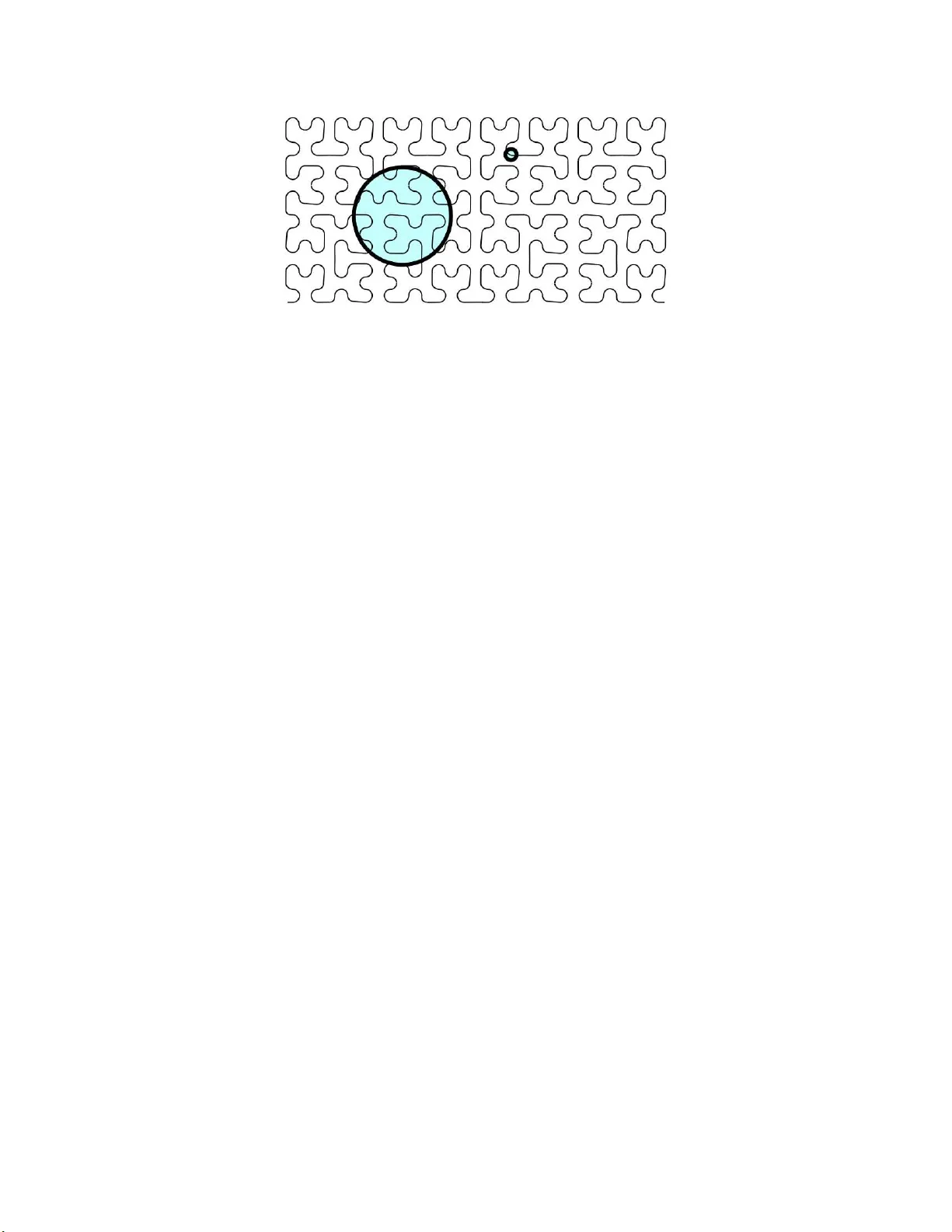
Random projection trees for v ector quantization Sanjoy Dasgupta and Y oav F reund ∗ October 25, 2018 Abstract A simple and computationally efficient scheme for tree-structured vector quantization is presented. Unlike pre- vious methods, it s quantization error depends only on the intrinsic dimension of the data distribu tion, rather than t he apparent dimension of the space in which the data happe n t o lie. 1 Introd uction For a distrib ution P on R D , the k th quan tization err or is commo nly defined as inf µ 1 ,...,µ k ∈ R D E  min 1 ≤ j ≤ k k X − µ j k 2  , where k · k denotes Euclidean norm and the expectation is over X drawn at random from P . It is known [15] that this infimum is re alized, thou gh perhap s not uniqu ely , by some set of p oints µ 1 , . . . , µ k , called a k - optimal set of centers . The r esulting q uantization error has been sho wn to be rou ghly k − 2 /D under a variety o f different assump tions o n P [8]. This is discouraging when D is high. For instance, if D = 1000 , it means that to merely halve the error, you need 2 500 times as many co dewords! In sho rt, vector quantization is susceptible to the same curse of d imensionality that has been the bane of other nonpa rametric statistical method s. A recen t po siti ve development in statistics and machin e learning has been the r ealization tha t a lot of data that superficially lie in a high-d imensional space R D , actu ally have lo w intrinsic dim ension, in the sense of lying close to a manifold of d imension d ≪ D . W e will g iv e several exam ples of this below . Ther e has th us been a huge interest in algo rithms that learn this manifold fro m data, with the intention th at futu re d ata can then be transformed into this low-dimensional s pace, in which the usual nonp arametric (and other) methods will work well [18, 16, 2]. In this pap er , we are interested in techniqu es tha t au tomatically ada pt to intrin sic low dimen sional stru cture withou t having to explicitly le arn this stru cture. W e describ e a tree- structured vector quantizer w hose quantiza tion error is k − 1 /O ( d ) ; that is to say , its error rate depends only on the low intrinsic dimension rather tha n the high appare nt dimension. The q uantizer is based on a hierarchica l decompo sition o f R D : first the entire space is split into two pieces, then each of these pieces is further split in two, and so on, until a partition of k cells is re ached. Each co dew ord is the mean of the distribution restricted to one of these cells. T ree-structured vector qu antizers abo und; the power of o ur appr oach comes fro m th e pa rticular splitting m ethod. T o di vide a r egion S into tw o, we pick a rando m d irection from the surface of th e unit sphere in R D , and split S at the median of its pr ojection onto this dir ection (Figure 1). W e c all the resulting spatial p artition a rando m pr o jection tr ee or RP tr ee . At first glan ce, it m ight seem th at a b etter way to sp lit a region is to find th e 2-o ptimal set of cen ters for it. Howe ver , as we explain below , this is an NP- hard optimization pro blem, and is ther efore un likely to be compu tationally tractable. Although there are sev eral algorithms that attemp t to solve this pro blem, such as Lloyd ’ s method [12, 11], they are not in general able to find the optimal solution. In fact, they are often far from optimal. ∗ Both authors are with the Departmen t of Computer Science and Engineering , Uni ver sity of Califo rnia, San Diego. Email: dasgupta,yfreu nd@cs.ucsd.edu . 1 Figure 1: Spatial partitionin g of R 2 induced by an RP tree with three levels. The dots ar e da ta po ints; each circle represents the mean of the vectors in one cell. For our random projection trees, we show tha t if the data h av e intrin sic dimen sion d (in a sense we m ake pre cise below), then each split p ares off about a 1 /d fractio n of the quantization error . Thus, after log k levels of sp litting, there are k cells and the quantizatio n error is of the form (1 − 1 /d ) log k = k − 1 /O ( d ) . There is no dependen ce at all on the extrinsic dimensionality D . 2 Detailed over view 2.1 Low-dimensional manif olds The increasing ubiquity of massive, high-d imensional data sets has fo cused the attention of the statistics and mach ine learning commu nities on the curse of dimension ality . A large part of this effort is based on exploiting the observation that many hig h-dimen sional da ta sets have low intrinsic dimension . This is a loo sely d efined notion, which is typically used to mean that the data lie near a smooth low-dimensional m anifold. For instan ce, suppose th at you wish to create realistic an imations by c ollecting human motion data an d then fitting models to it. A common meth od f or collecting motion data is to ha ve a person wear a skin-tight suit with h igh co ntrast referenc e p oints printed on it. V ideo cameras ar e used to tra ck the 3D trajectories of the ref erence points as the person is walking or run ning. In order to ensure good coverage, a typical suit has a bout N = 100 referen ce points. The position an d p osture of the body at a particular point of time is represented by a (3 N ) -dimension al vector . Howe ver , despite this seem ing h igh dimensionality , th e num ber o f degrees of freedom is small, cor respond ing to the dozen -or-so joint angles in the b ody . Th e positions o f the refe rence poin ts a re more or less deterministic fun ctions of these joint angles. Interestingly , in this examp le the intrin sic dimen sion b ecomes even smaller if we double th e dimen sion of th e embedd ing space by including for each sensor its relati ve velo city vecto r . In this space of dimension 6 N the measured points will lie very close to the one dimension al manif old d escribing the combina tions of locations and speeds th at the limbs go throug h during walking or running. T o take another example, a speech signal is comm only rep resented by a high -dimension al time series: the signal is broken into overlapping windows, and a variety of filters are applied within each window . Even richer representations can be obtained b y using m ore filters, or by concatenating vector s co rrespon ding to con secutiv e wind ows. Throu gh all this, the intrinsic dimensio nality remains small, because the system can be described by a few physical parameters describing the configu ration o f the speaker’ s vocal apparatus. In machine learn ing and statistics, almost all th e work on exploiting intrinsic low dimensionality consists of algo- rithms fo r learn ing the stru cture o f these manifolds; or more precisely , for learning e mbeddin gs of these manifo lds into low-dimensional Eu clidean space. Our contribution is a simple and compact data structure that automatically exploits the low intr insic dimen sionality of da ta o n a lo cal lev el without h aving to explicitly learn the glob al manifold stru cture. 2 Figure 2: Hilbert’ s space filling cu rve. Large n eighbor hoods loo k 2 -dimensiona l, smaller neighbor hoods loo k 1 - dimensiona l, and e ven smaller neig hborh oods would con sist mostly of m easuremen t noise and would there fore again be 2 -dimen sional. 2.2 Defining intrinsic dimensionality Low-dimensional manifold s are ou r insp iration and sour ce of intuition , but when it co mes to pr ecisely de fining intrin sic dimension for data analysis, th e d ifferential geometr y concep t of manifold is not entirely suitable. First o f a ll, an y data set lies o n a on e-dimen sional manifold, as evidenced by th e constru ction of sp ace-filling curves. Therefo re, some bound on curvature is implicitly needed. Second, and m ore impo rtant, it is unreason able to expect data to lie e xactly on a low-dimensional man ifold. At a certain small resolution , m easuremen t er ror and noise make a ny data set full- dimensiona l. The most we can ho pe is that the data d istribution is concentrated n ear a low-dimensional manifold of bound ed curv ature (Figure 2). W e ad dress these v arious con cerns with a statisti cally-motivated notio n of dimension: we say tha t a set S has local covariance d imension ( d, ǫ, r ) if neighborh oods of radius r have (1 − ǫ ) fraction of the ir v ariance con centrated in a d -dimension al su bspace. T o make this p recise, start by letting σ 2 1 , σ 2 2 , . . . , σ 2 D denote the eigen values of the covariance matrix; these are the variances in each of the eigenvector directio ns. Definition 1 Set S ⊂ R D has local covarianc e dimension ( d, ǫ, r ) if its res triction to any ball o f radius r has covari- ance matrix whose lar gest d eigenvalues satisfy σ 2 1 + · · · + σ 2 d ≥ (1 − ǫ ) · ( σ 2 1 + · · · + σ 2 D ) . 2.3 Random pr ojection trees Our new data stru cture, the ran dom projectio n tree, is built by rec ursiv e binary splits. The co re tree-building algo- rithm is called M A K E T R E E , which ta kes as input a d ata set S ⊂ R D , an d rep eatedly calls a splitting subr outine C H O O S E R U L E . procedure M A K E T R E E ( S ) if | S | < M inS iz e t hen retur n ( Leaf ) Rul e ← C H O O S E R U L E ( S ) Lef tT ree ← M A K E T R E E ( { x ∈ S : R ul e ( x ) = tr ue } ) Rig htT r ee ← M A K E T R E E ( { x ∈ S : R ul e ( x ) = f alse } ) return ([ Rul e, L ef tT r ee, R ig htT r ee ]) The RP tree has tw o types o f split. T ypically , a direction is chosen u niform ly at ran dom fr om surface of the unit sphere and the cell is split at its median , by a hyperplane orthog onal to this directio n. Occasio nally , a different ty pe of split is used, in which a cell is split into two pieces based on distance from the mean. 3 procedure C H O O S E R U L E ( S ) if ∆ 2 ( S ) ≤ c · ∆ 2 A ( S ) then  choose a random unit direction v Rul e ( x ) := x · v ≤ median ( { z · v : z ∈ S } ) else  Rul e ( x ) := k x − mean ( S ) k ≤ med ian ( {k z − m ean ( S ) k : z ∈ S } ) return ( Rul e ) In the code, c is a constant, ∆( S ) is th e diameter o f S (the distance between the two furthest points in the set), and ∆ A ( S ) is the a verag e diameter , that is, the a verage distance between points of S : ∆ 2 A ( S ) = 1 | S | 2 X x,y ∈ S k x − y k 2 . 2.4 Main r esult Suppose an RP tr ee is built f rom a data set S ⊂ R D , not n ecessarily finite. If the tree h as k levels, then it pa rtitions the space into 2 k cells. W e define the r adius of a cell C ⊂ R D to be the sma llest r > 0 su ch that S ∩ C ⊂ B ( x, r ) fo r some x ∈ C . Recall that an RP tree has two dif ferent types of split; let’ s call them splits by distance and splits by pr ojection . Theorem 2 The r e are consta nts 0 < c 1 , c 2 , c 3 < 1 with the fo llowing p r o perty . Su ppose an RP tree is b uilt using data set S ⊂ R D . Consider any cell C of radius r , such th at S ∩ C h as local covariance dimension ( d, ǫ, r ) , where ǫ < c 1 . Pick a point x ∈ S ∩ C at random, and let C ′ be the cell that contains it at the next level do wn. • I f C is split by distance, E [∆( S ∩ C ′ )] ≤ c 2 ∆( S ∩ C ) . • I f C is split by pr ojection, then E  ∆ 2 A ( S ∩ C ′ )  ≤ (1 − ( c 3 /d )) ∆ 2 A ( S ∩ C ) . In both cases, the expectation is over th e randomization in splitting C and the choice of x ∈ S ∩ C . 2.5 The hardness of finding optimal centers Giv en a data set, the optim ization pro blem of finding a k -o ptimal set of cen ters is called the k - means pro blem. Here is the formal definition. k - M E A N S C L U S T E R I N G Input: Set of points x 1 , . . . , x n ∈ R D ; integer k . Output: A p artition of th e points into clu sters C 1 , . . . , C k , along with a center µ j for each cluster , so as to minimize k X j =1 X i ∈ C j k x i − µ j k 2 . The typical method of appr oaching this task is to apply Lloyd’ s algorithm [12, 11], and usually this algorithm is itself called k -mea ns. The distinction between th e two is particularly imp ortant to make because Lloyd’ s algorith m is a heuristic th at often return s a suboptimal solution to the k - means p roblem. Indeed , its solution is often very far from optimal. What’ s worse, th is su boptimality is not just a problem with Lloyd’ s algorithm, but an in herent d ifficulty in the optimization task. k - M E A N S C L U S T E R I N G is an NP-h ard op timization prob lem, which means that it is very unlikely that th ere exists an efficient algorith m for it. T o expla in this a bit more clearly , we delve b riefly in to the theory of computatio nal complexity . The run ning time of an a lgorithm is typically measured as a f unction of its inp ut/outpu t size. In the case of k - means, for in stance, it would be given as a function of n , k , and D . An efficient algorithm is one whose r unning time 4 scales p olynomially with the pr oblem size. For instanc e, ther e are algorithms for sorting n numbers which take time propo rtional to n log n ; th ese qualify as ef ficient because n log n is bounde d above by a p olynom ial in n . For s ome optimization problems, the best algorithms we kno w t ake time e xponential in problem s ize. The famous trav eling salesman problem (given distanc es b etween n cities, plan a circular ro ute th rough them so that each city is visited o nce and the overall tour length is minim ized) is on e of these. There are various algorithms for it that take time propor tional to 2 n (or worse): this m eans each additional city causes the ru nning time to be doubled ! Even small graphs are therefore hard to solve. This disturbing lack of an efficient algorithm is not limited to just a few patholog ical optim ization tasks. Rather , it is an ep idemic across the en tire spectru m of compu tational tasks, one that a fflicts thousands of the pro blems we mo st urgently want to solve. Amazingly , it has been shown that the fates of these diverse problems (called NP-comple te problem s) ar e linked: eith er all of th em admit ef ficient algorithms, or none of t hem do! The mathematical community strongly believes th e latter to be the case, althou gh it is has n ot been proved. Resolving this question is o ne of th e se ven “grand challenges” of the ne w millenium identified by the Clay Institute. In Appendix II, we show th e following. Theorem 3 k - M E A N S C L U S T E R I N G is an NP-hard optimization p r o blem, even if k is r estricted to 2. Thus we cannot expect to be able to find a k -optim al set of c enters; the best we can hope is to find some set of centers that achieves ro ughly the optimal quantization error . 2.6 Related work Quantizatio n The litera ture on vector q uantization is substantial; see the wond erful survey o f Gray and Neuho ff [9] f or a com- prehen si ve overview . In th e most b asic setu p, there is som e distrib ution P over R D from which r andom vecto rs ar e generated and o bserved, an d the go al is to pick a fin ite codebook C ⊂ R D and an e ncoding function α : R D → C such that x ≈ α ( x ) for typical vectors x . Th e quantization error is usually m easured by squ ared lo ss, E k X − α ( X ) k 2 . An obvious ch oice is to let α ( x ) be the nearest n eighbor of x in C . Howe ver , the num ber o f codewords is of ten so enormo us that this nearest n eighbor computation cann ot be performed in real time. A more ef ficient s cheme is to have the codewords ar ranged in a tree [4]. The asymptotic behavior of qu antization error , assuming optimal quantizers and u nder various con ditions on P , has be en studied in gr eat detail. A n ice overview is p resented in the re cent mon ograph of Gr af and L uschgy [8]. The rates obtained fo r k -o ptimal quantizers are generally of the form k − 2 /D . There is also work on the spec ial case of data that lie exactly on a manifold, and who se d istribution is within some constant factor of unif orm; in suc h cases, rates of th e f orm k − 2 /d are obtained, wher e d is the dimension of th e m anifold. Our setting is considerab ly more general than this: we do not assum e op timal qu antization ( which is NP-hard), we ha ve a b road no tion of intrinsic dim ension that allows po ints to merely be clo se to a manifold rath er than on it, and we make no other assumptions abou t the distribution P . Compressed s ensing The field of c ompressed sen sing h as grown out of the surprising re alization that hig h-dimen sional sparse data can be accurately reconstructed from ju st a f ew rand om p rojection s [ 3, 5]. The central p remise of this research ar ea is that the original data thus nev er e ven n eeds to be collected: all one ever sees are the rand om projections. RP trees are similar in spirit an d entirely compatible with this v iewpoint. Th eorem 2 holds even if th e rando m projection s are f orced to be the same across ea ch en tire level of the tree. For a tree of depth k , this m eans o nly k random projec tions are ever needed, and th ese can be comp uted beforehan d (the split-by-d istance can be reworked to operate in the projected space rather than the high-d imensional s pace). The data are not accessed in any other w ay . 5 3 An RP tree ad apts to intrinsic dimension An RP tr ee has tw o varieties of split. If a cell C has mu ch larger diam eter th an average-diame ter (a verage interpoin t distance), then it is split accordin g to the distances of points from the mean. Otherwise, a random projectio n is used. The first type of split is particularly easy to analyze. 3.1 Splitting by distance fr om the mean This o ption is inv oked when the po ints in the cu rrent cell, c all them S , satisfy ∆ 2 ( S ) > c ∆ 2 A ( S ) ; recall that ∆( S ) is the diameter of S while ∆ 2 A ( S ) is the average interpoint distance. Lemma 4 Sup pose that ∆ 2 ( S ) > c ∆ 2 A ( S ) . Let S 1 denote the po ints in S whose d istance to mean ( S ) is less than or equal to th e median d istance, and let S 2 be the r ema ining p oints. Then the expected squar ed diameter after th e split is | S 1 | | S | ∆ 2 ( S 1 ) + | S 2 | | S | ∆ 2 ( S 2 ) ≤  1 2 + 2 c  ∆ 2 ( S ) . The proof of this lemma is deferred to the Appendix, as are most of the other proofs in this paper . 3.2 Splitting by proje ction: pr oof outline Suppose th e cur rent cell c ontains a set of po ints S ⊂ R D for which ∆ 2 ( S ) ≤ c ∆ 2 A ( S ) . W e will show that a split by projection has a constant probab ility of red ucing the a verage squ ared diameter ∆ 2 A ( S ) by Ω(∆ 2 A ( S ) /d ) . Our proo f has three parts: I. Supp ose S is split into S 1 and S 2 , with mea ns µ 1 and µ 2 . T hen the r eduction in average diam eter can be expressed in a remarka bly s imple form, as a multiple of k µ 1 − µ 2 k 2 . II. Next, we gi ve a lower b ound o n the distance between th e p r o jected m eans, ( e µ 1 − e µ 2 ) 2 . W e show that the distribution of the projected points is subgaussian with variance O (∆ 2 A ( S ) /D ) . Th is well-behavedness i mplies that ( e µ 1 − e µ 2 ) 2 = Ω(∆ 2 A ( S ) /D ) . III. W e finish by showing that, approximately , k µ 1 − µ 2 k 2 ≥ ( D /d )( e µ 1 − e µ 2 ) 2 . This is because µ 1 − µ 2 lies close to the subspace sp anned by th e top d e igenv ectors of the covariance matrix of S ; and with high prob ability , every vector in this subspace shrinks by O ( p d/D ) when projected on a random line. W e now tac kle these three parts of the proof in order . 3.3 Quantifying the red uction in av erage diameter The a verage squar ed d iameter ∆ 2 A ( S ) has certain reformulatio ns that make it convenient to work with. These prop- erties are con sequences of the following two observations, th e first of which the read er ma y recognize as a standard “bias-variance” decomposition of statis tics. Lemma 5 Let X , Y be in depend ent and identically distributed random variables in R n , an d let z ∈ R n be any fixed vector . (a) E  k X − z k 2  = E  k X − E X k 2  + k z − E X k 2 . (b) E  k X − Y k 2  = 2 E  k X − E X k 2  . Pr oof. Part (a) is immed iate when b oth sides are exp anded. For (b), we use p art ( a) to assert that fo r any fixed y , we have E  k X − y k 2  = E  k X − E X k 2  + k y − E X k 2 . W e th en take expectation over Y = y . This can be u sed to show that th e av eraged squar ed diamete r , ∆ 2 A ( S ) , is twice th e average squared d istance of p oints in S from their mean. 6 Corollary 6 The average squar ed diameter of a set S can also be written as: ∆ 2 A ( S ) = 2 | S | X x ∈ S k x − m ean ( S ) k 2 . Pr oof. ∆ 2 A ( S ) is simply E  k X − Y k 2  , when X , Y are i.i.d. draws from the uniform distrib ution over S . At each successi ve level of the tree, the current cell is split into tw o, either by a random projection or according to distance from the mean. Sup pose th e po ints in the curr ent cell ar e S , and that they are split into sets S 1 and S 2 . It is obvious that the expected diameter is nonincr easing: ∆( S ) ≥ | S 1 | | S | ∆( S 1 ) + | S 2 | | S | ∆( S 2 ) . This is also true of the expected av erage diameter . In fact, we can prec isely characterize how mu ch it decreases on account of the split. Lemma 7 Sup pose s et S is partitione d (in any manner) i nto S 1 and S 2 . Then ∆ 2 A ( S ) −  | S 1 | | S | ∆ 2 A ( S 1 ) + | S 2 | | S | ∆ 2 A ( S 2 )  = 2 | S 1 | · | S 2 | | S | 2 k mean ( S 1 ) − me an ( S 2 ) k 2 . This completes part I of the proof outline. 3.4 Pr operties of random pr ojections Our quantization scheme d epends heavily up on c ertain regularity pro perties o f random p rojection s. W e now re vie w these properties, which are critical for parts II and III of our proof. The most o bvious way to pick a random pr ojection from R D to R is to choose a p rojection dire ction u unifo rmly at rando m from the surface of the unit sphere S D − 1 , and to send x 7→ u · x . Another comm on optio n is to select the projectio n vector fro m a mu ltiv ariate Gaussian distribution, u ∼ N (0 , (1 / D ) I D ) . This g i ves almost the same distribution as befo re, and is sligh tly easier to work with in terms of the algorithm and analysis. W e will therefore use this type of projection, bearing in mind th at all proof s carr y over to the other v ariety as well, with slight changes in constants. The key p roperty of a ran dom pr ojection f rom R D to R is that it approximately pr eserves the lengths o f vectors, modulo a scaling factor of √ D . This is summarized in the lemma below . Lemma 8 F ix any x ∈ R D . Pick a r andom vector U ∼ N (0 , (1 /D ) I D ) . Then for any α, β > 0 : (a) P h | U · x | ≤ α · k x k √ D i ≤ q 2 π α (b) P h | U · x | ≥ β · k x k √ D i ≤ 2 β e − β 2 / 2 Lemma 8 app lies to any individual vector . Thus it also app lies, in expectation, to a vector chosen at ran dom from a set S ⊂ R D . Applying Marko v’ s inequality , we can then conclud e that when S is projected o nto a rand om d irection, most of the projected points will be close together, in a cen tral in terval of size O (∆( S ) / √ D ) . Lemma 9 Sup pose S ⊂ R D lies within so me ball B ( x 0 , ∆) . Pick an y 0 < δ, ǫ ≤ 1 su ch that δǫ ≤ 1 /e 2 . Let ν be any measur e on S . Then with p r o bability > 1 − δ over the choice of rando m pr oje ction U onto R , a ll but an ǫ fraction of U · S (me asur ed accor ding to ν ) lies within distance q 2 ln 1 δǫ · ∆ √ D of U · x 0 . 7 As a corollary , the median of the projected poin ts must also lie within this central interval. Corollary 10 Under the hy potheses of Lemma 9, for an y 0 < δ < 2 /e 2 , the following ho lds with pr obability at lea st 1 − δ over the choice of pr ojection: | median ( U · S ) − U · x 0 | ≤ ∆ √ D · r 2 ln 2 δ . Pr oof. Let ν b e the uniform distrib ution over S and use ǫ = 1 / 2 . Finally , we examine wh at hap pens when the set S is a d -dim ensional subsp ace o f R D . Lem ma 8 tells us that th e projection of a ny specific vector x ∈ S is unlikely to have length too mu ch greater than k x k / √ D , with hig h prob ability . A slightly weaker bo und can be shown to hold for all of S simultan eously; the proof tec hnique has appeared b efore in se veral contexts, including [14, 1]. Lemma 11 Ther e e xists a co nstant κ 1 with the fo llowing p r o perty . F ix a ny δ > 0 and a ny d -dimensional su bspace H ⊂ R D . Pic k a random pr oje ction U ∼ N (0 , (1 /D ) I D ) . Then with pr obability at least 1 − δ over the c hoice of U , sup x ∈ H | x · U | 2 k x k 2 ≤ κ 1 · d + ln 1 /δ D . Pr oof. It is enou gh to show that the inequa lity ho lds fo r S = H ∩ (surface of the unit sphere in R D ). Let N b e any (1 / 2 ) -cover of th is set; it is po ssible to achie ve | N | ≤ 10 d [13]. Apply Lemma 8, along with a union b ound , to conclud e th at with probab ility a t least 1 − δ ov er th e choice of projection U , sup x ∈ N | x · U | 2 ≤ 2 · ln | N | + ln 1 /δ D . Now , define C b y C = sup x ∈ S  | x · U | 2 · D ln | N | + ln 1 /δ  . W e’ll com plete th e pr oof by showing C ≤ 8 . T o th is end , pick the x ∗ ∈ S for which th e sup remum is realized (note S is compact) , a nd choose y ∈ N whose distance to x ∗ is at most 1 / 2 . Then, | x ∗ · U | ≤ | y · U | + | ( x ∗ − y ) · U | ≤ r ln | N | + ln 1 /δ D  √ 2 + 1 2 √ C  From the definition of x ∗ , it follows that √ C ≤ √ 2 + √ C / 2 a nd thus C ≤ 8 . 3.5 Pr operties of the project ed data Projection from R D into R 1 shrinks the average squared d iameter of a data set by roug hly D . T o see this, we start with the fact that when a data set with covariance A is projected onto a vector U , the pro jected data have variance U T AU . W e now show that for rando m U , such quad ratic forms are concentrated about their expected values. Lemma 12 Supp ose A is an n × n positive semidefinite matrix, and U ∼ N (0 , (1 /n ) I n ) . Then for any α, β > 0 : (a) P [ U T AU < α · E [ U T AU ]] ≤ e − ((1 / 2) − α ) / 2 , and (b) P [ U T AU > β · E [ U T AU ]] ≤ e − ( β − 2) / 4 . 8 Lemma 13 Pick U ∼ N (0 , (1 /D ) I D ) . Then for an y S ⊂ R D , with pr obability at least 1 / 10 , the pr ojectio n of S onto U ha s average squa r ed diameter ∆ 2 A ( S · U ) ≥ ∆ 2 A ( S ) 4 D . Pr oof. By Coro llary 6, ∆ 2 A ( S · U ) = 2 | S | X x ∈ S (( x − m ean ( S )) · U ) 2 = 2 U T cov ( S ) U. where cov ( S ) is the covariance o f data set S . Th is quadratic term has expectation ( over choice of U ) E [2 U T cov ( S ) U ] = 2 X i,j E [ U i U j ] cov ( S ) ij = 2 D X i cov ( S ) ii = ∆ 2 A ( S ) D . Lemma 12(a) then bound s the proba bility that it is much smaller than its expected v alue. Next, we examine the ov erall d istribution o f the projected points. When S ⊂ R D has diameter ∆ , its p rojection into the line c an have diameter upto ∆ , but as we saw in L emma 9, most of it will lie within a central inter val of size O (∆ / √ D ) . What can be said about points that fall outside this interval? Lemma 14 Supp ose S ⊂ B (0 , ∆) ⊂ R D . Pic k any δ > 0 and c hoose U ∼ N (0 , (1 /D ) I D ) . Then with pr obability at least 1 − δ over the choice o f U , the pr ojection S · U = { x · U : x ∈ S } satisfies the following pr operty for all po sitive inte gers k . The fraction of points outside the interval  − k ∆ √ D , + k ∆ √ D  is at most 2 k δ · e − k 2 / 2 . Pr oof. This fo llows by apply ing Lemm a 9 f or each p ositiv e integer k (with co rrespon ding failure pro bability δ / 2 k ), and then taking a union bound . 3.6 Distance between the pr ojected means W e are dealing with the case when ∆ 2 ( S ) ≤ c · ∆ 2 A ( S ) , t hat is, the diam eter of set S is at most a constant factor time s the av erage interp oint d istance. If S is projected onto a ran dom dir ection, th e pro jected p oints will ha ve variance abo ut ∆ 2 A ( S ) /D , by Lemma 13; and b y Lemma 14, it isn’t to o far from the truth to think o f these points as ha ving rough ly a Gaussian distribution. Thu s, if the pro jected points are split into two gr oups at the mean , we would expec t the means of these two groups t o be separated b y a distance of about ∆ A ( S ) / √ D . Indeed, this is th e case. Th e same holds if we split at the median, which isn’t all that dif ferent from the mean for close-to-Gaussian distrib utions. Lemma 15 Ther e is a co nstant κ 2 for whic h the following hold s. P ick any 0 < δ < 1 / 1 6 c . P ick U ∼ N (0 , (1 / D ) I D ) and split S into two pieces: S 1 = { x ∈ S : x · U < s } and S 2 = { x ∈ S : x · U ≥ s } , wher e s is eith er mean ( S · U ) or med ian ( S · U ) . Write p = | S 1 | / | S | , a nd let e µ 1 and e µ 2 denote th e mean s of S 1 · U and S 2 · U , respectively . Then with pr obability at least 1 / 10 − δ , ( e µ 2 − e µ 1 ) 2 ≥ κ 2 · 1 ( p (1 − p )) 2 · ∆ 2 A ( S ) D · 1 c log (1 /δ ) . 9 Pr oof. Let the rand om variable e X d enote a uniform -rando m draw fro m the projected points S · U . W ith out loss of generality m ean ( S ) = 0 , so that E e X = 0 and thus p e µ 1 + (1 − p ) e µ 2 = 0 . Rearranging, w e g et e µ 1 = − (1 − p )( e µ 2 − e µ 1 ) and e µ 2 = p ( e µ 2 − e µ 1 ) . W e alread y kn ow from Lemma 13 (and Corollary 6) that with pro bability at least 1 / 10 , the variance of the projected points is significant: var ( e X ) ≥ ∆ 2 A ( S ) / 8 D . W e’ll show this implies a similar lower bound on ( e µ 2 − e µ 1 ) 2 . Using 1 ( · ) to denote 0 − 1 indicator v ariables, var ( e X ) ≤ E [( e X − s ) 2 ] ≤ E [2 t | e X − s | + ( | e X − s | − t ) 2 · 1 ( | e X − s | ≥ t )] for any t > 0 . This is a convenient form ulation since the linear term gi ves u s e µ 2 − e µ 1 : E [2 t | e X − s | ] = 2 t ( p ( s − e µ 1 ) + (1 − p )( e µ 2 − s )) = 4 t · p (1 − p ) · ( e µ 2 − e µ 1 ) + 2 ts (2 p − 1) . The last term vanishes since the split is either at the mea n of the projected poin ts, in w hich case s = 0 , or a t the median, in which case p = 1 / 2 . Next, we’ ll choose t = t o ∆( S ) √ D · r log 1 δ for some suitable co nstant t o , so t hat the quadratic term in var ( e X ) can be boun ded using Lemma 14 and Cor ollary 10: with probability at least 1 − δ , E [( | e X | − t ) 2 · 1 ( | e X | ≥ t )] ≤ δ · ∆ 2 ( S ) D (this is a simple integration). Putting the pieces together , we have ∆ 2 A ( S ) 8 D ≤ var ( e X ) ≤ 4 t · p (1 − p ) · ( e µ 2 − e µ 1 ) + δ · ∆ 2 ( S ) D . The result now follo ws immediately by algebraic manipu lation, using the relation ∆ 2 ( S ) ≤ c ∆ 2 A ( S ) . 3.7 Distance between the high-dimensional means Split S into two piec es as in the setting of Lemm a 15, and let µ 1 and µ 2 denote the m eans of S 1 and S 2 , respectively . W e a lready have a lower bound on the distanc e b etween the pr ojected mean s, e µ 2 − e µ 1 ; we will now sh ow that k µ 2 − µ 1 k is larger than this by a factor o f about p D /d . Th e m ain technical dif ficulty here is the dep endence b etween the µ i and the projection U . I ncidentally , this is the on ly part of the entire argument that exploits intrinsic dimensionality . Lemma 16 Ther e exists a co nstant κ 3 with the following pr operty . Suppo se set S ⊂ R D is such tha t the top d eigen values of cov ( S ) accou nt for mor e than 1 − ǫ of its trace. Pick a random vector U ∼ N (0 , (1 /D ) I D ) , an d split S in to two p ieces, S 1 and S 2 , in any fashion ( which ma y depend u pon U ) . Let p = | S 1 | / | S | . Let µ 1 and µ 2 be the means of S 1 and S 2 , and let e µ 1 and e µ 2 be the means of S 1 · U and S 2 · U . Then, for any δ > 0 , with pr obability at least 1 − δ over the choice of U , k µ 2 − µ 1 k 2 ≥ κ 3 D d + ln 1 / δ  ( e µ 2 − e µ 1 ) 2 − 4 p (1 − p ) ǫ ∆ 2 A ( S ) δ D  . Pr oof. Assume witho ut loss of g enerality that S has zero mean. Let H denote the sub space spanned by the top d e igenv ectors of the covariance matrix o f S , and let H ⊥ be its orthog onal subspace. Write any point x ∈ R D as x H + x ⊥ , where each compon ent is s een as a vector in R D that lies in the respective subsp ace. Pick the random vector U ; with probability ≥ 1 − δ it satisfies the following two prop erties. 10 Property 1: For some constant κ ′ > 0 , fo r e very x ∈ R D | x H · U | 2 ≤ k x H k 2 · κ ′ · d + ln 1 /δ D ≤ k x k 2 · κ ′ · d + ln 1 / δ D . This holds (with probab ility 1 − δ / 2 ) by Lemma 11. Property 2: Letting X d enote a uniform-r andom d raw from S , we ha ve E X [( X ⊥ · U ) 2 ] ≤ 2 δ · E U E X [( X ⊥ · U ) 2 ] = 2 δ · E X E U [( X ⊥ · U ) 2 ] = 2 δ D · E X [ k X ⊥ k 2 ] ≤ ǫ ∆ 2 A ( S ) δ D . The first step is Markov’ s in equality , and holds with p robability 1 − δ / 2 . The last inequality comes fr om the local covariance con dition. So assume the two properties hold. Writing µ 2 − µ 1 as ( µ 2 H − µ 1 H ) + ( µ 2 ⊥ − µ 1 ⊥ ) , ( e µ 2 − e µ 1 ) 2 = (( µ 2 H − µ 1 H ) · U + ( µ 2 ⊥ − µ 1 ⊥ ) · U ) 2 ≤ 2(( µ 2 H − µ 1 H ) · U ) 2 + 2(( µ 2 ⊥ − µ 1 ⊥ ) · U ) 2 . The first term can be boun ded by Pr operty 1: (( µ 2 H − µ 1 H ) · U ) 2 ≤ k µ 2 − µ 1 k 2 · κ ′ · d + ln 1 / δ D . For the second term, let E X denote expectation o ver X chosen unifo rmly a t random from S . Then (( µ 2 ⊥ − µ 1 ⊥ ) · U ) 2 ≤ 2( µ 2 ⊥ · U ) 2 + 2( µ 1 ⊥ · U ) 2 = 2( E X [ X ⊥ · U | X ∈ S 2 ]) 2 + 2( E X [ X ⊥ · U | X ∈ S 1 ]) 2 ≤ 2 E X [( X ⊥ · U ) 2 | X ∈ S 2 ] + 2 E X [( X ⊥ · U ) 2 | X ∈ S 1 ] ≤ 2 1 − p · E X [( X ⊥ · U ) 2 ] + 2 p · E X [( X ⊥ · U ) 2 ] = 2 p (1 − p ) E X [( X ⊥ · U ) 2 ] ≤ 2 p (1 − p ) · ǫ ∆ 2 A ( S ) δ D . by Property 2. The lemma follows by putting the v arious pieces t ogether . W e can now finish off the proof of Theorem 2. Theorem 17 F ix any ǫ ≤ O (1 /c ) . Suppo se set S ⊂ R D has t he pr operty that the top d eigenvalues of cov ( S ) acco unt for mor e than 1 − ǫ of its trace. Pick a random vector U ∼ N (0 , (1 /D ) I D ) and split S into two parts, S 1 = { x ∈ S : x · U < s } and S 2 = { x ∈ S : x · U ≥ s } , wher e s is either mean ( S · U ) or median ( S · U ) . Th en with p r o bability Ω(1 ) , the expected average diameter shrinks by Ω(∆ 2 A ( S ) /cd ) . Pr oof. By Lem ma 7, the reduction in e xpected av erage diameter is ∆ 2 A ( S ) −  | S 1 | | S | ∆ 2 A ( S 1 ) + | S 2 | | S | ∆ 2 A ( S 2 )  = 2 | S 1 | · | S 2 | | S | 2 k mean ( S 1 ) − me an ( S 2 ) k 2 , or 2 p (1 − p ) k µ 1 − µ 2 k 2 in the language of Lemmas 15 and 16. The rest follows fr om those two lemmas. 11 Acknowledgements Dasgupta acknowledges the suppo rt of the National Science Foundation under grants IIS-034764 6 and IIS-0 71354 0. Refer ences [1] R. Baraniuk, M. Da venport, R. DeV ore, and M. W akin. A simple proof of the restricted isometry property f or random matrices. Constructive App r oximation , 2008. [2] M. Belkin an d P . Niyogi. L aplacian eig enmaps fo r d imensionality redu ction and data representatio n. Neural Computation , 15(6):1 373– 1396, 2 003. [3] E. Cande s and T . T ao. Near op timal signal rec overy f rom rando m projections: univ ersal encoding strategies? IEEE T ransactions on Informatio n Theory , 52(1 2):5406 –5425, 2 006. [4] P .A. Cho u, T . Loo kabaug h, and R.M. Gray . Optim al pru ning with applications to tr ee-structured sou rce c oding and modeling. I EEE T ransactions on Information Theory , 35(2):2 99–31 5, 1 989. [5] D. Donoho . Com pressed sensing. IEE E T ransactions on Information Theory , 52(4):12 89–13 06, 20 06. [6] P . Dr ineas, A. Frieze, R. Kannan, S. V empala, and V . V inay . Clustering large g raphs via the singular value decomp osition. Machine Learning , 56:9–3 3, 2004. [7] R. Durrett. P r o bability: Theory and Examples . Du xbury , s econd edition , 1995. [8] S. Graf and H. Luschgy . F ou ndation s of qu antization for pr oba bility distrib utions . Spring er , 2 000. [9] R.M. Gray and D.L. Neuho ff. Quan tization. IEEE T r ansactions on Informatio n Theo ry , 4 4(6):2 325–2 383, 1998. [10] J.B. Krusk al and M. W ish. Multidimensional Scaling . Sag e Univ ersity Paper series on Quantitative App lication in the Social Sciences, 07-01 1. 1 978. [11] S.P . Lloyd. Least sq uares quantization in pcm. IEEE T ransactions on Information Theo ry , 2 8(2):1 29–13 7, 198 2. [12] J.B. MacQueen. Some methods for classification a nd analysis of multi variate ob servations. In Pr oceedings o f F ifth Berkeley Sympo sium on Mathematical S tatistics a nd Pr obability , volume 1, pages 28 1–297 . Univ ersity of California Press, 1967. [13] J. Matou sek. Lectur es on Discr e te Geometry . Sp ringer, 200 2. [14] V .D. Milman. A ne w pro of o f th e th eorem of a. dvoretsky on sections of con ve x bod ies. Functional An alysis a nd its Application s , 5 (4):28 –37, 1971. [15] D. Pollard. Quantizatio n an d th e m ethod o f k -m eans. IEEE T ransactions o n In formation Theo ry , 28:199–20 5, 1982. [16] S.T . Roweis an d L.K. Saul. Nonlinear dimen sionality re duction by lo cally linear embedd ing. Science , (290) :2323– 2326, 2000. [17] I.J. Schoenberg. Metric spaces and positive definite functions. T ransaction s of the American Mathematical Society , 44:522 –553, 1 938. [18] J. T enen baum, V . de Silva, and J. La ngford . A glo bal geom etric framework for no nlinear dimensionality red uc- tion. S cience , 290(55 00):23 19–2323, 2 000. 12 4 A ppen dix I: Proofs of main theorem 4.1 Pr oof of Lemma 8 Since U has a Ga ussian distrib ution, and any lin ear combination o f independ ent Gau ssians is a Gaussian, it follows that the pro jection U · x is also Gau ssian. Its mea n and variance are ea sily seen to be zero and k x k 2 /D , r espectively . Therefo re, writing Z = √ D k x k ( U · x ) we hav e that Z ∼ N (0 , 1) . The bound s stated in the lemma n ow follow from pro perties o f the stan dard normal. I n particular, N (0 , 1) is roughly flat in the range [ − 1 , 1] and then drops o ff ra pidly; the two cases in th e lemma statem ent correspo nd to these two regimes. The highest den sity ach iev ed by the standard nor mal is 1 / √ 2 π . Thus the p robab ility m ass i t assigns to the interval [ − α, α ] is at most 2 α/ √ 2 π ; this takes care of (a). For (b), we use a standard tail bound for the normal, P ( | Z | ≥ β ) ≤ (2 /β ) e − β 2 / 2 ; see, for instance, page 7 of [7]. 4.2 Pr oof of Lemma 9 Set c = p 2 ln 1 / ( δ ǫ ) ≥ 2 . Fix any po int x , and ran domly choo se a projection U . Le t e x = U · x (and likewise, let e S = U · S ). What is the chance that e x lands far from e x 0 ? Define the bad e vent to be F x = 1 ( | e x − e x 0 | ≥ c ∆ / √ D ) . By Lemma 8(b), we have E U [ F x ] ≤ P U  | e x − e x 0 | ≥ c · k x − x 0 k √ D  ≤ 2 c e − c 2 / 2 ≤ δǫ . Since this h olds for any x ∈ S , it also ho lds in expectation over x drawn fr om ν . W e are interested in boun ding the probab ility (over the cho ice o f U ) th at mo re th an an ǫ fraction o f ν falls far fr om e x 0 . Using Markov’ s inequality and then Fubini’ s t heorem , we have P U [ E µ [ F x ] ≥ ǫ ] ≤ E U [ E µ [ F x ]] ǫ = E µ [ E U [ F x ]] ǫ ≤ δ , as claimed. 4.3 Pr oof of Lemma 4 Let random variable X be distributed u niform ly over S . T hen P  k X − E X k 2 ≥ median ( k X − E X k 2 )  ≥ 1 2 by definition of median, so E  k X − E X k 2  ≥ med ian ( k X − E X k 2 ) / 2 . It follows from Corollary 6 that median ( k X − E X k 2 ) ≤ 2 E  k X − E X k 2  = ∆ 2 A ( S ) . Set S 1 has squared d iameter ∆ 2 ( S 1 ) ≤ (2 median ( k X − E X k )) 2 ≤ 4∆ 2 A ( S ) . Mea nwhile, S 2 has squared diameter at most ∆ 2 ( S ) . Therefore, | S 1 | | S | ∆ 2 ( S 1 ) + | S 2 | | S | ∆ 2 ( S 2 ) ≤ 1 2 · 4∆ 2 A ( S ) + 1 2 ∆ 2 ( S ) and the lemma follows by using ∆ 2 ( S ) > c ∆ 2 A ( S ) . 13 4.4 Pr oof of Lemma 12 This follows b y examining the moment-ge nerating f unction of U T AU . Since the d istribution of U is spher ically symmetric, we can work in th e eige nbasis o f A and assume without loss of g enerality th at A = diag ( a 1 , . . . , a n ) , where a 1 , . . . , a n are the eigen values. Mo reover , for convenience we take P a i = 1 . Let U 1 , . . . , U n denote the ind ividual coordinates of U . W e ca n rewrite them as U i = Z i / √ n , wh ere Z 1 , . . . , Z n are i.i.d. standard normal rando m variables. Thus U T AU = X i a i U 2 i = 1 n X i a i Z 2 i . This tells us immediately that E [ U T AU ] = 1 /n . W e use Chern off ’ s b oundin g meth od for both parts. For ( a), for any t > 0 , P  U T AU < α · E [ U T AU ]  = P " X i a i Z 2 i < α # = P h e − t P i a i Z 2 i > e − tα i ≤ E h e − t P i a i Z 2 i i e − tα = e tα Y i E h e − ta i Z 2 i i = e tα Y i  1 1 + 2 ta i  1 / 2 and the rest follows by using t = 1 / 2 along with the in equality 1 / (1 + x ) ≤ e − x/ 2 for 0 < x ≤ 1 . Similarly for (b ), for 0 < t < 1 / 2 , P  U T AU > β · E [ U T AU ]  = P " X i a i Z 2 i > β # = P h e t P i a i Z 2 i > e tβ i ≤ E h e t P i a i Z 2 i i e tβ = e − tβ Y i E h e ta i Z 2 i i = e − tβ Y i  1 1 − 2 ta i  1 / 2 and it is adequa te to cho ose t = 1 / 4 and in v oke the inequality 1 / (1 − x ) ≤ e 2 x for 0 < x ≤ 1 / 2 . 4.5 Pr oof of Lemma 7 Let µ, µ 1 , µ 2 denote the means of S , S 1 , and S 2 . Using Corollary 6 and Lemma 5(a), we have ∆ 2 A ( S ) − | S 1 | | S | ∆ 2 A ( S 1 ) − | S 2 | | S | ∆ 2 A ( S 2 ) = 2 | S | X S k x − µ k 2 − | S 1 | | S | · 2 | S 1 | X S 1 k x − µ 1 k 2 − | S 2 | | S | · 2 | S 2 | X S 2 k x − µ 2 k 2 = 2 | S | ( X S 1  k x − µ k 2 − k x − µ 1 k 2  + X S 2  k x − µ k 2 − k x − µ 2 k 2  ) = 2 | S 1 | | S | k µ 1 − µ k 2 + 2 | S 2 | | S | k µ 2 − µ k 2 . Writing µ as a weighted a verage of µ 1 and µ 2 then completes the proof. 14 5 A ppen dix II: Hardness of k -m eans clustering k - M E A N S C L U S T E R I N G Input: Set of points x 1 , . . . , x n ∈ R d ; integer k . Output: A p artition of th e points into clu sters C 1 , . . . , C k , along with a center µ j for each cluster , so as to minimize k X j =1 X i ∈ C j k x i − µ j k 2 . (Here k · k is Euclidean distan ce.) It can b e ch ecked that in any op timal solu tion, µ j is th e mean of the po ints in C j . Thus the { µ j } c an be removed en tirely from the formulation of the problem. From Lemma 5(b), X i ∈ C j k x i − µ j k 2 = 1 2 | C j | X i,i ′ ∈ C j k x i − x i ′ k 2 . Therefo re, t he k -means cost functio n can equiv alently be re written as k X j =1 1 2 | C j | X i,i ′ ∈ C j k x i − x i ′ k 2 . W e co nsider the specific case when k is fixed to 2. Theorem 18 2 -means clustering is an NP-har d optimization pr ob lem. This was recently asserted in [6], but the proof was fla wed. W e establish ha rdness b y a sequence o f red uctions. Ou r starting point is a standard restriction of 3 S AT that is well known to be NP-comp lete. 3 S A T Input: A Boolean formu la in 3CNF , where each clause h as exactly three literals and each v ariable appear s at least twice. Output: true if formula is satis fiable, false if not. By a standard r eduction from 3 S AT , we show that a special case of N OT - A L L - E Q U A L 3 S A T is also hard. For com- pleteness, the details are laid out in the next section. N A E S A T * Input: A Boolean f ormula φ ( x 1 , . . . , x n ) in 3CNF , such that (i) every clause contains exactly thr ee literals, and (ii) each pair of variables x i , x j appears together in at most two clauses, once as either { x i , x j } or { x i , x j } , and once as either { x i , x j } or { x i , x j } . Output: true if th ere exists an a ssignment in which e ach clause co ntains exactly one o r two satisfied literals; false o therwise. Finally , we get to a gener alization of 2 - M E A N S . G E N E R A L I Z E D 2 - M E A N S Input: An n × n matr ix of interpoint distances D ij . Output: A partition of the points into two clusters C 1 and C 2 , so as to minimize 2 X j =1 1 2 | C j | X i,i ′ ∈ C j D ii ′ . 15 W e reduc e N A E S A T * to G E N E R A L I Z E D 2 - M E A N S . For any input φ to N A E S A T * , we s how h ow to ef ficiently produ ce a distanc e matr ix D ( φ ) and a threshold c ( φ ) such th at φ satisfies N A E S A T * if and o nly if D ( φ ) ad mits a gen eralized 2-means clustering of cost ≤ c ( φ ) . Thus G E N E R A L I Z E D 2 - M E A N S C L U S T E R I N G is hard. T o g et back to 2 - M E A N S (an d thus establish Theo rem 18), we prove that the distance matrix D ( φ ) can in fact be realized by sq uared Euclidean distances. This existential fact is also con structive, because in such cases, the embedding ca n be obtained in cubic time by classical multidimensional scaling [10]. 5.1 Hardness of N A E S A T * Giv en an input φ ( x 1 , . . . , x n ) to 3 S AT , we first construct an intermediate formula φ ′ that is satisfiable if and only if φ is, and ad ditionally has exactly three occurre nces of each variable: one in a clause o f size three, and two in clau ses of size two. This φ ′ is then used to produ ce a n input φ ′′ to N A E S AT * . 1. Construc ting φ ′ . Suppose variable x i appears k ≥ 2 tim es in φ . Crea te k variables x i 1 , . . . , x ik for use in φ ′ : use the same clauses, but rep lace each occurrence of x i by one of the x ij . T o enfo rce agreement between the different copies x ij , add k a dditional clauses ( x i 1 ∨ x i 2 ) , ( x i 2 ∨ x i 3 ) , . . . , ( x ik , x i 1 ) . Th ese co rrespon d to the implications x 1 ⇒ x 2 , x 2 ⇒ x 3 , . . . , x k ⇒ x 1 . By design, φ is satis fiable if and only if φ ′ is satisfiable. 2. Construc ting φ ′′ . Now we constru ct an input φ ′′ for N A E S AT * . Suppose φ ′ has m clauses with three literals and m ′ clauses with two literals. Crea te 2 m + m ′ + 1 new variables: s 1 , . . . , s m and f 1 , . . . , f m + m ′ and f . If the j th three-literal c lause in φ ′ is ( α ∨ β ∨ γ ) , rep lace it with two clauses in φ ′′ : ( α ∨ β ∨ s j ) and ( s j ∨ γ ∨ f j ) . If the j th tw o-literal clause in φ ′ is ( α ∨ β ) , replace it with ( α ∨ β ∨ f m + j ) in φ ′′ . Finally , ad d m + m ′ clauses that enforce agreement among the f i : ( f 1 ∨ f 2 ∨ f ) , ( f 2 ∨ f 3 ∨ f ) , . . . , ( f m + m ′ ∨ f 1 ∨ f ) . All clauses in φ ′′ have exactly thre e literals. Moreover , the o nly pairs o f variables that o ccur togeth er (in clau ses) more than once are { f i , f } pairs. Each such pair occur s twice, as { f i , f } and { f i , f } . Lemma 19 φ ′ is satisfiable if and only if φ ′′ is not-all-eq ual satisfia ble. Pr oof. First sup pose that φ ′ is satisfiable. Use t he same settings of th e variables f or φ ′′ . Set f = f 1 = · · · = f m + m ′ = false . For the j th three-literal clause ( α ∨ β ∨ γ ) o f φ ′ , if α = β = fal se th en set s j to true , otherwise set s j to false . The resulting assignment satisfies exactly one or two literals of each clause in φ ′′ . Con versely , suppose φ ′′ is not- all-equal satisfi able. W ithout loss of gen erality , the satisfying assignm ent has f set to false (o therwise flip all assignments). The clau ses of the form ( f i ∨ f i +1 ∨ f ) then enforce agreement amo ng all the f i variables. W e can assume they are all fa lse (other wise, once aga in, flip all a ssignments). This mea ns the two-literal clauses o f φ ′ must be satisfied. Finally , consider any three-literal clau se ( α ∨ β ∨ γ ) of φ ′ . This was rep laced by ( α ∨ β ∨ s j ) and ( s j ∨ γ ∨ f j ) in φ ′′ . Since f j is false , it f ollows that one of th e literals α, β , γ mu st be satisfied. Thus φ ′ is satisfied. 5.2 Hardness of G E N E R A L I Z E D 2 - M E A N S Giv en an instan ce φ ( x 1 , . . . , x n ) of N A E S A T * , we co nstruct a 2 n × 2 n distance matrix D = D ( φ ) wher e the (imp licit) 2 n points co rrespon d to literals. En tries of this matrix will be ind exed as D α,β , fo r α, β ∈ { x 1 , . . . , x n , x 1 , . . . , x n } . Another bit of notation: we write α ∼ β to mean that either α and β occur togeth er in a clause o r α and β o ccur together in a clau se. For in stance, the clau se ( x ∨ y ∨ z ) allows o ne to assert x ∼ y but n ot x ∼ y . The in put restrictions on N A E S AT * ensure that e very relatio nship α ∼ β is genera ted by a uniq ue clau se; it is not possible to have two different clauses that both contain either { α, β } or { α, β } . 16 Define D α,β =        0 if α = β 1 + ∆ if α = β 1 + δ if α ∼ β 1 otherwise Here 0 < δ < ∆ < 1 ar e constants such that 4 δ m < ∆ ≤ 1 − 2 δ n , where m is the nu mber of clauses of φ . On e valid setting is δ = 1 / (5 m + 2 n ) and ∆ = 5 δ m . Lemma 20 If φ is a satisfia ble in stance of N A E S A T * , then D ( φ ) a dmits a generalized 2-mean s clustering of cost c ( φ ) = n − 1 + 2 δ m/n , wher e m is th e number of clauses of φ . Pr oof. The obviou s clu stering is to m ake one cluster (say C 1 ) consist of the positive literals in the satisfy ing not- all-equal assignmen t and the other clu ster ( C 2 ) the n egati ve literals. Each cluster ha s n points, and the distance between any two d istinct points α, β within a cluster is either 1 or, if α ∼ β , 1 + δ . Each clause o f φ h as at least one literal in C 1 and at least one literal in C 2 , since it is a n ot-all-equ al assignment. Hence it contributes exactly one ∼ pair to C 1 and one ∼ pair to C 2 . T he figure below sho ws an e xample with a clause ( x ∨ y ∨ z ) and assi gnmen t x = t rue , y = z = false . C 1 C 2 z x x y z y Thus the clustering cost is 1 2 n X i,i ′ ∈ C 1 D ii ′ + 1 2 n X i,i ′ ∈ C 2 D ii ′ = 2 · 1 n  n 2  + mδ  = n − 1 + 2 δ m n . Lemma 21 Let C 1 , C 2 be any 2-clu stering of D ( φ ) . If C 1 contains both a v ariable an d its negation, then the cost of this clustering is at least n − 1 + ∆ / (2 n ) > c ( φ ) . Pr oof. Supp ose C 1 has n ′ points while C 2 has 2 n − n ′ points. Since all d istances are a t least 1 , and since C 1 contains a pair of points at distance 1 + ∆ , the total clustering cost is at least 1 n ′  n ′ 2  + ∆  + 1 2 n − n ′  2 n − n ′ 2  = n − 1 + ∆ n ′ ≥ n − 1 + ∆ 2 n . Since ∆ > 4 δ m , this is always more than c ( φ ) . 17 Lemma 22 If D ( φ ) admits a 2-clustering of cost ≤ c ( φ ) , then φ is a satisfiable instance of N A E S A T * . Pr oof. Let C 1 , C 2 be a 2-clustering of cost ≤ c ( φ ) . By the previous lemma, neither C 1 nor C 2 contain both a variable and its negation. Thus | C 1 | = | C 2 | = n . The cost of the clustering can be written as 2 n    n 2  + δ X clauses  1 if clause split between C 1 , C 2 3 otherwise    Since th e cost is ≤ c ( φ ) , it f ollows that all clau ses ar e split b etween C 1 and C 2 , that is, every clause has at least o ne literal in C 1 and one literal in C 2 . T herefor e, the assignm ent that sets all of C 1 to tru e and all of C 2 to fal se is a valid N A E S A T * a ssignment for φ . 5.3 Embeddability of D ( φ ) W e now show that D ( φ ) can be embe dded into l 2 2 , in the sense that there exist points x α ∈ R 2 n such that D α,β = k x α − x β k 2 for all α, β . W e rely upon the following classical result [17]. Theorem 23 (Schoenberg) Let H denote the matrix I − (1 / N ) 11 T . An N × N symmetric ma trix D can b e embedded into l 2 2 if and only if − H D H is positive semidefinite. The following c orollary is immediate. Corollary 24 An N × N symmetric matrix D ca n be embedded into l 2 2 if and only if u T D u ≤ 0 for a ll u ∈ R N with u · 1 = 0 . Pr oof. Since th e range of the map v 7→ H v is precisely { u ∈ R N : u · 1 = 0 } , we hav e − H D H is positive sem idefinite ⇔ v T H D H v ≤ 0 fo r all v ∈ R N ⇔ u T D u ≤ 0 fo r all u ∈ R N with u · 1 = 0 . Lemma 25 D ( φ ) can be embedded into l 2 2 . Pr oof. I f φ is a f ormula with variables x 1 , . . . , x n , then D = D ( φ ) is a 2 n × 2 n matrix wh ose first n rows/column s correspo nd to x 1 , . . . , x n and remaining rows/columns co rrespon d to x 1 , . . . , x n . The entry for literals ( α, β ) is D αβ = 1 − 1 ( α = β ) + ∆ · 1 ( α = β ) + δ · 1 ( α ∼ β ) , where 1 ( · ) denotes the indicator function. Now , pick any u ∈ R 2 n with u · 1 = 0 . Let u + denote the first n coordinates of u an d u − the last n coordinates. u T D u = X α,β D αβ u α u β = X α,β u α u β  1 − 1 ( α = β ) + ∆ · 1 ( α = β ) + δ · 1 ( α ∼ β )  = X α,β u α u β − X α u 2 α + ∆ X α u α u α + δ X α,β u α u β 1 ( α ∼ β ) ≤ X α u α ! 2 − k u k 2 + 2∆( u + · u − ) + δ X α,β | u α || u β | ≤ −k u k 2 + ∆( k u + k 2 + k u − k 2 ) + δ X α | u α | ! 2 ≤ − (1 − ∆) k u k 2 + 2 δ k u k 2 n where the last step uses the Cauchy-Schwarz inequality . Since 2 δ n ≤ 1 − ∆ , this qu antity is alw ays ≤ 0 . 18