Complexity Analysis of Reed-Solomon Decoding over GF(2^m) Without Using Syndromes

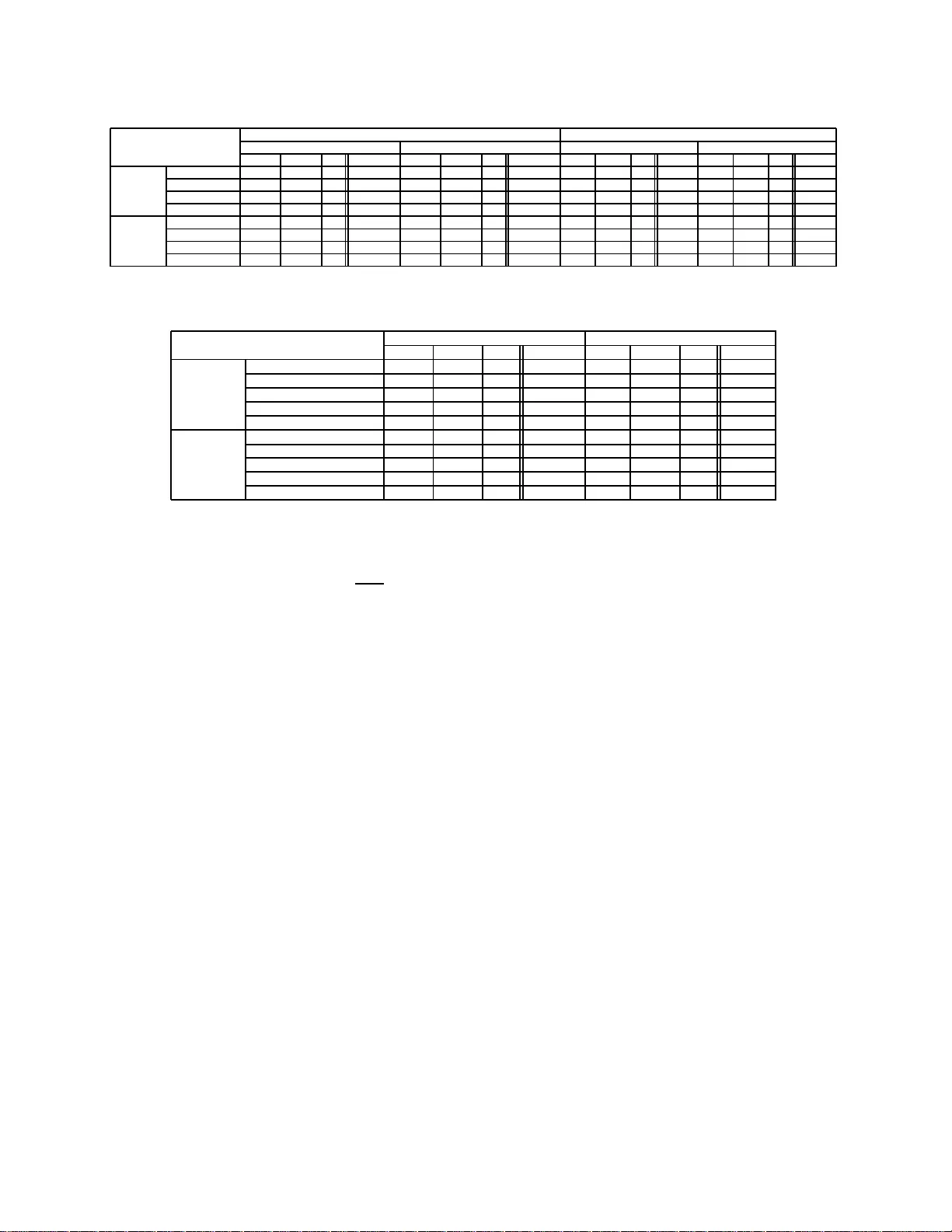
1 Comple xity Analysis of Reed–Solomon Decoding o v er GF(2 m ) W ithout Using Syndromes Ning Chen and Zh iyuan Y an Department of Electrical a nd Computer Enginee ring Lehigh Univ ersity , Bethlehem, Penn sylvania 18015, USA E-mail: { nic6, yan } @lehigh. edu Abstract — There has been renewed interest in decodin g Reed– Solomon (RS) codes without usin g syndromes rece ntly . In th is paper , we inv estigate the complexity of syndromeless decoding, and compare it to that of syndrome-base d d ecoding. Aiming to p ro vide guidelines to practical applications, our complexity analysis fo cuses on RS codes ov er characteristic-2 fields, for which some multiplicative FFT techniques ar e not applicable. Due to moderate block lengths of RS codes in p ractice, our analysis is complete, without big O notation. In addition to fast implementation usin g additive FFT techn iques, we also consider direct implementation, wh ich i s still rele vant for RS codes with moderate lengths. F or high rate RS co des, when compared to syndrome-based decoding algorithms, not only syndro meless decoding algorithms require more field operations regardless of implementation, but also decoder architectures based on th eir direct impl ementation s hav e higher hardwar e costs and lower throughput. W e also derive tighter b ounds on the complexities of fast polynomial multipli cations based on Cantor’s approach and the fast extended Eu cl i dean algo rithm. Index T erms — Reed–Solomon codes, Decoding, Complexity theory , Galois fields, Discrete Fourier transforms, Polynomials I . I N T RO D U C T I O N Reed–Solomo n (RS) codes are among the most widely used error contr ol codes, with applications in space co mmun ica- tions, wireless co mmunica tions, and c onsumer electronics [1 ]. As such, efficient deco ding of RS codes is of great interest. The majority of the application s of RS codes use syndrom e- based decodin g algorithm s such as the Berlekamp –Massey algorithm (BMA) [2 ] or the extended Eu clidean algor ithm (EEA) [3]. Altern ativ e hard decision deco ding m ethods fo r RS codes with out using syndro mes were consider ed in [4]– [6]. As pointed out in [7 ], [8], the se algorithms belong to the class of frequency-d omain algorithm s and are related to the W elch–Berlekamp algorithm [9]. In contrast to synd rome- based decod ing algorithms, th ese algor ithms do not compute syndrom es a nd av oid the Chie n search a nd Forney’ s formula . Clearly , this difference leads to the question whether these al- gorithms offer lower complexity than syn drome- based decod- ing, especially w hen fast F ourier transform (FFT) tech niques are applied [6]. Asymptotic complexity of syndrom eless deco ding was an- alyzed in [6] , and in [7] it was co ncluded that synd romeless decodin g h as the same asymptotic complexity O ( n log 2 n ) 1 The material in this paper was presente d in part at the IEEE W orkshop on Signal Processi ng Systems, Shanghai, China , Oct ober 2007. 1 Note that all the logarith ms in this paper are to base two . as syndro me-based decoding [10]. Howe ver , existing asymp- totic comp lexity analysis is limited in sev eral aspects. For example, for RS co des over Fermat fields GF(2 2 r + 1) and other prim e fields [5], [6], efficient mu ltiplicativ e FFT technique s lea d to an asymptotic com plexity of O ( n log 2 n ) . Howe ver , such FFT techniques do no t apply to ch aracteristic- 2 fields, and hen ce this c omplexity is no t a pplicable to RS codes over cha racteristic-2 fields. For RS codes ov er arb itrary fields, the asymptotic complexity of syndromeless decoding based on multiplicative FFT technique s was sh own to be O ( n log 2 n log log n ) [6 ]. Althoug h they are applica ble to RS codes over characteristic-2 fields, the co mplexity has large coefficients and multiplicativ e FFT tec hniques are less effi - cient th an fast implementatio n based o n a dditive FFT f or RS codes with m oderate block leng ths [6], [11], [1 2]. As such, asymptotic co mplexity analysis p rovides little h elp to practical applications. In this p aper, we an alyze the co mplexity of syndro meless decodin g and co mpare it to th at of syndro me-based decodin g. Aiming to provide guidelines to system de signers, we f ocus on th e deco ding comp lexity o f RS codes ov er GF(2 m ) . Since RS codes in p ractice hav e m oderate lengths, our complex- ity an alysis provid es not only the co efficients f or the most significant terms, but also the following terms. Due to their moderate leng ths, our compar ison is ba sed on two types of implementatio ns o f syn dromeless decod ing and syndro me- based decodin g: direc t implemen tation and fast implem en- tation based on FFT techniqu es. D irect implemen tations are often efficient when decodin g RS cod es with moderate leng ths and have wid espread applicatio ns; thus, we co nsider both computatio nal com plexities, in terms of field operations, and hardware costs and throughpu ts. For fast im plementation s, we consider their computation al complexities on ly an d their hard- ware imp lementation s are beyond the sco pe of th is paper . W e use additive FFT techniques based on Can tor’ s appr oach [13] since this approach achieves small coefficients [6 ], [11] and hence is more suitable for moderate lengths. In con trast to some previous work s [ 12], [14], wh ich co unt field m ultiplica- tions an d additio ns togethe r , we differentiate the multiplicative and add itiv e complexities in o ur analysis. The main contributions of the pape rs are: • W e derived a tighter bou nd on th e complexities of fast polyno mial multiplication based on Cantor’ s app roach; • W e also obtained a tig hter boun d on the complexity o f the fast extended Euclidean algorithm (FEEA) for general 2 partial gre atest common d ivisor (GCD) computatio n; • W e evaluated the com plexities o f syndr omeless d ecod- ing based on different imp lementation approaches and compare them w ith their c ounterp arts of syndrome-ba sed decodin g; Both errors-only and errors-and -erasures de- coding are considered. • W e compare the hardware costs and thro ughpu ts of direct implementatio ns for syndro meless deco ders with th ose for syn drome- based d ecoders. The rest o f the pap er is organized as follows. T o make this paper self-contain ed, in Section I I we briefly revie w FFT algorithm s over finite fields, fas t algor ithms for poly nomial multiplication and division over GF(2 m ) , the FEEA, and syndrom eless de coding algorithms. Sectio n III presents both computatio nal complexity and decoder a rchitectures o f d irect implementatio ns of syndromeless decoding, and compare them with their coun terparts fo r syndrom e-based deco ding a lgo- rithms. Section IV compares the co mputation al complexity of fast implemen tations of syndr omeless decoding with that of syndrom e-based deco ding. In Section V, case studies on two RS codes a re provided and error s-and-era sures decoding is discussed. The conclusions are g iv en in Section VI. I I . B AC K G R O U N D A. F ast F ourier T ransform Over F inite F ields For a ny n ( n | q − 1 ) distinct elements a 0 , a 1 , . . . , a n − 1 ∈ GF( q ) , th e transform from f = ( f 0 , f 1 , . . . , f n − 1 ) T to F ,  f ( a 0 ) , f ( a 1 ) , . . . , f ( a n − 1 )  T , whe re f ( x ) = P n − 1 i =0 f i x i ∈ GF( q )[ x ] , is called a discrete Fourier transform (DFT), de- noted by F = DFT( f ) . Accordingly , f is called the inverse DFT of F , deno ted by f = IDFT( F ) . Asymp totically fast Fourier transform (FFT) algorithm over GF (2 m ) was proposed in [1 5]. Redu ced-com plexity cycloto mic FFT ( CFFT) was shown to be ef ficient for moderate lengths in [ 16]. B. P olyn omial Multiplication Over GF(2 m ) B y Cantor’s Ap- pr o ach A fast polynom ial multiplication algorith m using ad ditive FFT was prop osed by Cantor [1 3] for GF( q q m ) , wh ere q is prime, and it was generalized to GF( q m ) in [11] . Instead of ev aluating and interpo lating over the multiplicative subgrou ps as in multiplicative FFT te chnique s, Cantor’ s ap proach uses additive subg roups. Can tor’ s appr oach relies on two alg o- rithms: multipoint e valuation (MPE) [11, Algorithm 3 .1] and multipoint interp olation (MPI) [1 1, Algor ithm 3.2]. Suppose th e degree of the p roduct of two po lynomials over GF(2 m ) is less than h ( h ≤ 2 m ), th e product can be obtained as follows: First, the two operand polyn omials are ev aluated using the MPE algorithm; The ev aluation results are then m ultiplied point-wise; Fin ally the p roduc t polyno mial is obtained by the MPI alg orithm to interpolate the point- wise m ultiplication results. The polyno mial multiplication requires at m ost 3 2 h log 2 h + 15 2 h log h + 8 h mu ltiplications over GF(2 m ) and 3 2 h log 2 h + 29 2 h log h + 4 h + 9 additions over GF(2 m ) [11]. For simplicity , hencefor th in this paper, all arithmetic operations are ov er GF(2 m ) unless specified otherwise. C. P olyno mial Division By Newton Iteration Suppose a, b ∈ GF( q )[ x ] are two polynomials of degrees d 0 + d 1 and d 1 ( d 0 , d 1 ≥ 0) , respectively . T o find the q uotient polyno mial q an d the remain der po lynomia l r satisfying a = q b + r wh ere deg r < d 1 , a fast polyno mial division algo - rithm is a vailable [12] . Suppose rev h ( a ) , x h a ( 1 x ) , the fast algorithm first com putes the inv erse of rev d 1 ( b ) mo d x d 0 +1 by Newton iteration. Then the rev erse quotient is gi ven by q ∗ = rev d 0 + d 1 ( a )rev d 1 ( b ) − 1 mo d x d 0 +1 . Finally , the actual quotient and remainde r are given b y q = rev d 0 ( q ∗ ) an d r = a − q b . Thus, the com plexity of polyno mial di vision with remain der of a polynomial a of degree d 0 + d 1 by a monic poly nomial b of degree d 1 is at mo st 4 M ( d 0 ) + M ( d 1 ) + O ( d 1 ) multip lica- tions/addition s when d 1 ≥ d 0 [12, Th eorem 9.6] , where M ( h ) stands for th e numbers of mu ltiplications/additio ns required to multiply two po lynom ials of degree less th an h . D. F ast Extended Eu clidean Algorithm Let r 0 and r 1 be two monic polyno mials with deg r 0 > deg r 1 and we assume s 0 = t 1 = 1 , s 1 = t 0 = 0 . Step i ( i = 1 , 2 , · · · , l ) of the EEA computes ρ i +1 r i +1 = r i − 1 − q i r i , ρ i +1 s i +1 = s i − 1 − q i s i , and ρ i +1 t i +1 = t i − 1 − q i t i so that th e sequence r i are mon ic polynomials with strictly d ecreasing degrees. If the GCD of r 0 and r 1 is desired, the EEA terminates whe n r l +1 = 0 . For 1 ≤ i ≤ l , R i , Q i · · · Q 1 R 0 , where Q i =  0 1 1 ρ i +1 − q i ρ i +1  and R 0 =  1 0 0 1  . T hen it can be easily verified th at R i =  s i t i s i +1 t i +1  for 0 ≤ i ≤ l . In RS decodin g, the E EA stops when the degree of r i falls below a cer tain thr eshold for the first time, and we refer to this as partial GCD. The FEEA in [12], [17] costs no mor e than  22 M ( h ) + O ( h )  log h multiplications/ad ditions wh en n 0 ≤ 2 h [1 4]. E. Syndr ome-ba sed an d Syn dr o meless Decoding Over a finite field GF( q ) , suppose a 0 , a 1 , . . . , a n − 1 are n ( n ≤ q ) distinct elements and g 0 ( x ) , Q n − 1 i =0 ( x − a i ) . Let us consider an RS code over GF( q ) with length n , dimension k , a nd minim um Hamming distance d = n − k + 1 . A message polyno mial m ( x ) of degree less than k is en coded to a codeword ( c 0 , c 1 , · · · , c n − 1 ) with c i = m ( a i ) , and the received vector is gi ven by r = ( r 0 , r 1 , · · · , r n − 1 ) . The syndr ome-b ased hard decision decoding consists of the following steps: syndro me computation , ke y equatio n solver , the Chien search, and Forney’ s formula. Further details are omitted, and interested readers are referred to [1], [2], [18]. W e also conside r the follo wing tw o syndr omeless algorithms: Algorithm 1: [4 ], [5] , [6, Alg orithm 1] 1.1 Interpolation : Construct a poly nomial g 1 ( x ) with deg g 1 ( x ) < n such that g 1 ( a i ) = r i for i = 0 , 1 , . . . , n − 1 . 1.2 Partial GCD: Apply the EEA to g 0 ( x ) and g 1 ( x ) , an d find g ( x ) and v ( x ) that maximize deg g ( x ) while satis fy- ing v ( x ) g 1 ( x ) ≡ g ( x ) mo d g 0 ( x ) and deg g ( x ) < n + k 2 . 3 1.3 Message Recovery: If v ( x ) | g ( x ) , th e message poly- nomial is recovered by m ( x ) = g ( x ) v ( x ) , otherwise outp ut “decodin g failure. ” Algorithm 2: [6, Algo rithm 1a] 2.1 Interpolation : Construct a poly nomial g 1 ( x ) with deg g 1 ( x ) < n such that g 1 ( a i ) = r i for i = 0 , 1 , . . . , n − 1 . 2.2 Partial GCD: Find s 0 ( x ) and s 1 ( x ) satisfying g 0 ( x ) = x n − d +1 s 0 ( x )+ r 0 ( x ) an d g 1 ( x ) = x n − d +1 s 1 ( x )+ r 1 ( x ) , where deg r 0 ( x ) ≤ n − d and deg r 1 ( x ) ≤ n − d . Apply th e EEA to s 0 ( x ) and s 1 ( x ) , and stop when th e remainder g ( x ) ha s d egree less than d − 1 2 . Thus, we h av e v ( x ) s 1 ( x ) + u ( x ) s 0 ( x ) = g ( x ) . 2.3 Message Recovery: I f v ( x ) ∤ g 0 ( x ) , output “decoding failure”; otherwise, fir st co mpute q ( x ) , g 0 ( x ) v ( x ) , an d then obtain m ′ ( x ) = g 1 ( x ) + q ( x ) u ( x ) . If deg m ′ ( x ) < k , output m ′ ( x ) ; otherwise output “deco ding failure. ” Compared with Algo rithm 1, th e pa rtial GCD step of Al- gorithm 2 is simpler but its message recovery step is mo re complex [6]. I I I . D I R E C T I M P L E M E N TA T I O N O F S Y N D R O M E L E S S D E C O D I N G A. Complexity Analysis W e analyze the com plexity o f direct impleme ntation o f Algorithms 1 an d 2. For simplicity , we assume n − k is ev en and hen ce d − 1 = 2 t . First, g 1 ( x ) in Steps 1.1 and 2.1 is giv en by IDFT( r ) . Direct implemen tation of Steps 1.1 and 2.1 follows Ho rner’ s rule, and re quires n ( n − 1) m ultiplications an d n ( n − 1) additions [19 ]. Steps 1.2 and 2.2 both use the EEA. The Sugiyama tower (ST) [3], [20] is well known as an efficient dire ct imp lementa- tion of the EEA. F or Algorithm 1, the ST is initialized by g 1 ( x ) and g 0 ( x ) , whose degrees are at m ost n . Sin ce the nu mber of iterations is 2 t , Step 1 .2 requ ires 4 t ( n + 2) m ultiplications and 2 t ( n + 1 ) additions. For Algorithm 2, th e ST is initialized by s 0 ( x ) and s 1 ( x ) , whose degree s are at most 2 t and the iteration nu mber is a t most 2 t . Step 1.3 r equires one polyn omial di vision, which can be implemented b y u sing k iterations of cross multiplications in the ST . Since v ( x ) is ac tually th e error locato r p olynom ial [6], deg v ( x ) ≤ t . Hen ce, this requires k ( k + 2 t + 2 ) multiplication s and k ( t + 2 ) additions. Ho wev er, the result of th e polynom ial division is scaled by a n onzero constant. That is, cross multi- plications lead to ¯ m ( x ) = am ( x ) . T o remove the scaling factor a , we can first co mpute 1 a = lc( g ( x )) lc( ¯ m ( x ))lc( v ( x )) , where lc( f ) denotes the leading coefficient of a poly nomial f , and then obtain m ( x ) = 1 a ¯ m ( x ) . Th is process req uires one inversion and k + 2 multiplications. Step 2.3 in volves o ne poly nomial division, on e poly nomial multiplication, an d one poly nomial addition , and their c om- plexities depend on the d egrees of v ( x ) a nd u ( x ) , deno ted as d v and d u , respectively . In the polynomial di vision, let the result of the ST be ¯ q ( x ) = aq ( x ) . The scaling factor is r e- covered by 1 a = 1 lc( ¯ q ( x ))l c( v ( x )) . Thus it requires one inv ersion, ( n − d v + 1)( n + d v + 3) + n − d v + 2 multiplication s, an d ( n − d v + 1)( d v + 2) additions to obtain q ( x ) . Th e polyn omial multiplication needs ( n − d v + 1)( d u + 1 ) multip lications and ( n − d v + 1)( d u + 1) − ( n − d v + d u + 1) additions, and the polyn omial a ddition n eeds n addition s since g 1 ( x ) has degree at most n − 1 . The total complexity o f Step 2.3 includes ( n − d v + 1)( n + d v + d u + 5) + 1 multiplications, ( n − d v + 1 )( d v + d u + 2 ) + n − d u additions, a nd on e inversion. Consider the worst case for multiplicativ e co mplexity , where d v should be as small as possible. But d v > d u , so the highest multiplicative comp lexity is ( n − d u )( n + 2 d u + 6) + 1 , which maximizes when d u = n − 6 4 . And we know d u < d v ≤ t . Let R denote the code rate. So for RS c odes with R > 1 2 , the m aximum co mplexity is n 2 + nt − 2 t 2 + 5 n − 2 t + 5 multiplications, 2 nt − 2 t 2 + 2 n + 2 addition s, and one in version. For codes with R ≤ 1 2 , the maximum complexity is 9 8 n 2 + 9 2 n + 11 2 multiplications, 3 8 n 2 + 3 2 n + 3 2 additions, a nd one in version. T able I lists the comp lexity o f direct implemen tation of Algorithms 1 an d 2, in terms of oper ations in GF(2 m ) . Th e complexity of syndro me-based decodin g is given in T able II. The numbers for syndrome computation, the Chien search, and Forney’ s formula are from [21]. W e assume the EEA is used for the key equ ation solver since it was shown to b e equivalent to the BMA [22 ]. The ST is u sed to im plement th e E EA. Note that the overall complexity of syndrome-b ased d ecoding can be reduced b y sha ring computations b etween the Chie n search and F orney’ s formula. Howev er, th is is not taken into account in T able II. B. Complexity Comparison For any ap plication with fixed parameters n and k , the compariso n between the algorithms is straig htforward u sing the complexities in T ables I and II. Below we tr y to determine which algorithm is more suitable for a given code rate. The co mparison b etween different algorithm s is co mplicated by three different typ es of field op erations. Howe ver , th e complexity is domin ated by the number of multiplications: in hardware impleme ntation, both multiplication and inversion over GF(2 m ) req uires an area-time complexity of O ( m 2 ) [2 3], whereas an ad dition require s an area-time co mplexity of O ( m ) ; the com plexity due to in version s is negligible since the require d numb er of in versions is mu ch smaller than those of m ultiplications; the numbers of mu ltiplications and additions are both O ( n 2 ) . Th us, we focus on the num ber of multiplications for simplicity . Since t = 1 − R 2 n an d k = Rn , th e mu ltiplicativ e complexi- ties of Alg orithms 1 and 2 are (3 − R ) n 2 + (3 − R ) n + 2 and 1 2 (3 R 2 − 7 R + 8) n 2 + (7 − 3 R ) n + 5 , respectively , wh ile the complexity of syn drome- based decoding is 5 R 2 − 13 R +8 2 n 2 + (2 − 3 R ) n . It is ea sy to verify that in all these complexities, the quadratic an d linear coe fficients are of the same order of magnitud e; he nce, we consider only the quadratic ter ms. Con- sidering only th e quadr atic ter ms, Algorith m 1 is less efficient than synd rome-b ased d ecoding whe n R > 1 5 . If the Chien search and Forney’ s formula share compu tations, this thresho ld will be even lower . Compar ing th e highest terms, Algor ithm 2 is less efficient than the syndrome-b ased algor ithm regardless 4 T ABLE I D I R E C T I M P L E M E N TA T I O N C O M P L E X I T I E S O F S Y N D R O M E L E S S D E C O D I N G A L G O R I T H M S Multipl ications Addition s In ver sions Interpol ation n ( n − 1) n ( n − 1) 0 Parti al GCD Algorith m 1 4 t ( n + 2) 2 t ( n + 1) 0 Algorith m 2 4 t (2 t + 2) 2 t (2 t + 1) 0 Message Recov ery Algorith m 1 ( k + 2)( k + 1) + 2 kt k ( t + 2) 1 Algorith m 2 n 2 + nt − 2 t 2 + 5 n − 2 t + 5 2 nt − 2 t 2 + 2 n + 2 1 T otal Algorith m 1 2 n 2 + 2 nt + 2 n + 2 t + 2 n 2 + 3 nt − 2 t 2 + n − 2 t 1 Algorith m 2 2 n 2 + nt + 6 t 2 + 4 n + 6 t + 5 n 2 + 2 nt + 2 t 2 + n + 2 t + 2 1 T ABLE II D I R E C T I M P L E M E N TA T I O N C O M P L E X I T Y O F S Y N D R O M E - B A S E D D E C O D I N G Multipl ications Addition s In versions Syndrome Computation 2 t ( n − 1) 2 t ( n − 1) 0 Ke y Equatio n Solv er 4 t (2 t + 2) 2 t (2 t + 1) 0 Chien Searc h n ( t − 1) nt 0 Forne y’ s Formula 2 t 2 t (2 t − 1) t T otal 3 nt + 10 t 2 − n + 6 t 3 nt + 6 t 2 − t t of R . It is easy to verify that the most significan t term of the difference be tween Algorithms 1 and 2 is (1 − R )(3 R − 2) 2 n 2 . So when imp lemented directly , Algorith m 1 is less effi cient than Algorithm 2 when R > 2 3 . Thus, Algorithm 1 is mo re suitable for codes with very low r ate, wh ile syn drom e-based decod ing is the most efficient for high rate codes. C. Har dwar e Costs, Latency , and Thr oug hput W e hav e compared the computational comp lexities of syn- dromeless decoding algo rithms with those of syndrome-b ased algorithm s. Now we compare th ese two types of decoding algorithm s fr om a hardware persp ectiv e: we will com pare the hardware co sts, laten cy , and throug hput of decoder architec- tures based on d irect implem entations of th ese algorith ms. Since ou r go al is to com pare synd rome-b ased algor ithms with syndrom eless algorithms, we select our architectures so that the com parison is o n a level field . Thu s, among various decoder architectures a vailable for syn drome -based deco ders in the literature, we consider the hyp ersystolic ar chitecture in [20]. Not only is it an efficient architectur e for syndrome- based decod ers, some of its functio nal units can be easily adapted to implement syndro meless decoder s. Thus, decod er architecture s for bo th types of decod ing algorith ms have the same structu re with som e functio nal u nits the same; this allow us to focus on the difference between the two types of algorithms. For th e same reason , we do not try to optimize the har dware costs, latency , or thro ughpu t using circuit le vel technique s since such tech niques will benefit the architectures for bo th types of deco ding algorithms in a similar fashion a nd hence d oes not affect the comparison. The hyper systolic architecture [20] contains three functio nal units: the power sums tower ( PST) com puting the syndrom es, the ST solv ing the key equatio n, and the corr ection tower (CT) perfor ming the Chien searc h and Forney’ s form ula. The PST consists of 2 t systolic cells, each of which comprises of o ne multiplier, one adder, fi ve registers, an d o ne m ultiplexer . The ST has δ + 1 ( δ is the maximal degree of the input polynomials) systolic cells, each of which con tains one multiplier, one adder, five registers, and se ven multiplexers. The latency of the ST is 6 γ clo ck cycles [2 0], where γ is the nu mber of iterations. For the syndro me-based decode r ar chitecture, δ and γ are b oth 2 t . The CT co nsists of 3 t + 1 evaluation cells, two delay cells, alo ng with two joiner cells, wh ich also perfor m in versions. Each e valuation cell needs one mu ltiplier , one ad der, four registers, and o ne multip lexer . Each d elay cell needs one register . The tw o joiner cells altoge ther ne ed two m ultipliers, one inverter , and four registers. T ab le III summarizes the hard ware co sts of the d ecoder architec ture f or syndrom e-based dec oders described above. For each functional unit, we also list th e latency (in clock cycles), as well as the number of clock cycles it needs to p rocess one received word, which is proportion al to the in verse of the through put. In theory , th e computatio nal complexities o f steps of RS decoding depend on th e received word, and the total co mplexity is obtained by first computing the sum of com plexities for all the steps and then considering the worst case scenario (cf. Section III-A). In contrast, th e hardware co sts, laten cy , a nd throug hput of e very f unctiona l unit are dominate d by the worst case scenario; the number s in T able III all correspon d to the worst case scenar io. The c ritical pa th delay ( CPD) is th e same, T mult + T add + T mux , for the PST , ST , and CT . In additio n to the registers required by the PST , ST , a nd CT , the to tal numb er of registers in T a ble III also acco unt for the registers needed by the delay line called Main Street [2 0]. Both the PST and the ST can be ad apted to implement decoder architectur es fo r syndrom eless dec oding algorithm s. Similar to syndrome comp utation, interpolatio n in syn drome- less d ecoders can be implemente d by Horn er’ s ru le, and thus the PST can be easily adapted to implement this step. For the architectu res based on syn dromele ss de coding, the PST contains n cells, and the h ardware costs of each cell rem ain the same. The p artial GCD is im plemented by the ST . Th e ST can implement the polynom ial division in me ssage recovery as well. In Step 1.3, th e maximum polynom ial degree of th e polyno mial division is k + t and th e iteration n umber is at most k . As mentio ned in Section III-A, the degree of q ( x ) in Step 2.3 r anges from 1 to t . In the po lynom ial division g 0 ( x ) v ( x ) , the maxim um polyno mial degree is n an d the iter ation nu mber 5 T ABLE III D E C O D E R A R C H I T E C T U R E B A S E D O N S Y N D RO M E - B A S E D D E C O D I N G ( C P D I S T mult + T add + T mux ) Multipl iers Adders In verte rs Re gisters Muxes Latenc y Throughput − 1 Syndrome Computation 2 t 2 t 0 10 t 2 t n + 6 t 6 t Ke y Equatio n Solver 2 t + 1 2 t + 1 0 10 t + 5 14 t + 7 12 t 12 t Correct ion 3 t + 3 3 t + 1 1 12 t + 10 3 t + 1 3 t 3 t T otal 7 t + 4 7 t + 2 1 n + 53 t + 15 19 t + 8 n + 21 t 12 t is at most n − 1 . Gi ven the maximum polynom ial degree and iteration numb er , the har dware co sts and latency for the ST can be determined as for the syndr ome-b ased arch itecture. The o ther ope rations of syn drome less d ecoders do not have correspo nding functional units av ailable in the hypersy stolic architecture , an d we c hoose to implement them in a straightfor- ward w ay . In the polynom ial m ultiplication q ( x ) u ( x ) , u ( x ) has degree at most t − 1 and the prod uct h as degree at most n − 1 . Thus it c an be done by n multiply-a nd-accu mulate circu its, n registers in t cycles (see, e.g ., [24]). The polynom ial add ition in Step 2.3 can be done in one clock cycle with n ad ders and n registers. T o remove the scaling factor , Step 1.3 is implemented in four cycles with at most one inv erter, k + 2 multipliers, and k + 3 registers; Step 2.3 is implemented in th ree cycles with at most one in verter , n + 1 multipliers, and n + 2 registers. W e summarize the hardware costs, latency , an d throughp ut of the decod er a rchitectures based on Algo rithms 1 and 2 in T able IV. Now we compar e the hardware costs of the three deco der architecture s based on T ables III an d I V. Th e hard ware costs are measur ed by the number s of v arious basic circ uit elements. All three decoder ar chitectures need on ly one inv erter . T he syndrom e-based deco der architectur e req uires fewer multi- plexers than the decoder architecture based on Algo rithm 1, regardless of th e rate, and fewer multiplier s, adders, and reg- isters when R > 1 2 . The syndrome-b ased decoder arc hitecture requires fewer r egisters than the decod er architecture based on Algo rithm 2 when R > 21 43 , an d f ewer multipliers, adder s, and multiplexers regard less of the rate. Th us for high rate codes, the syndrome-b ased dec oder has lower hardware costs than syndro meless decod ers. The decoder ar chitecture based on Alg orithm 1 requires fewer mu ltipliers and adders than that based on Algorithm 2, regardless of the rate, but more registers and mu ltiplexers when R > 9 17 . In these algorithm s, each step starts with the results of the previous step. Due to this d ata dependency , the ir correspo nding function al units have to operate in a pip elined fashion. Thus the deco ding laten cy is simply the sum o f the latency of all the functio nal u nits. The decoder architecture based on Algorithm 2 h as the lo ngest latency , regard less of the rate. T he syndrom e-based decoder architecture has shorter latency than the d ecoder architectur e based on Alg orithm 1 when R > 1 7 . All thr ee decoder s hav e the same CPD, so the thro ughp ut is determ ined b y the numb er o f clock cycles. Since the function al un its in each decoder architecture are pipelined, the th rough put of each decoder architecture is determined by the f unctional unit that requires the largest number of cycles. Regardless of the rate, the decoder based on Algorithm 2 has the lowest throughpu t. When R > 1 2 , the syndr ome-based decoder architecture has higher throughp ut than the decode r architecture based on Algo rithm 1. When the rate is lo wer, they have the same thr oughp ut. Hence fo r hig h rate RS cod es, the syndro me-based de- coder architec ture requires less h ardware and ach iev es higher throug hput and shorter latency than those based on synd rome- less decod ing algorith ms. I V . F A S T I M P L E M E N TA T I O N O F S Y N D RO M E L E S S D E C O D I N G In this section, we impleme nt the thr ee steps of Algo- rithms 1 and 2—interpolatio n, partial GCD, an d message recovery—by fast algor ithms d escribed in Section II and eval- uate their com plexities. Since b oth the p olynom ial division by Newton iter ation and th e FEEA depend on efficient polynomial multiplication, the decoding comp lexity relies on the com - plexity o f polyn omial multip lication. Thus, in a ddition to field multiplications and additions, the co mplexities in this section are also expressed in terms of polyno mial multiplications. A. P olyn omial Multiplication W e first derive a tighter b ound on the c omplexity of the fast polyno mial multiplication based on Cantor’ s a pproac h. Let the degree o f the product of tw o polyn omials be less than n . The poly nomial mu ltiplication can be done by two FFTs and o ne inv erse FFT if length- n FFT is a vailable ov er GF(2 m ) , which re quires n | 2 m − 1 . If n ∤ 2 m − 1 , on e option is to pad the p olynom ials to length n ′ ( n ′ > n ) with n ′ | 2 m − 1 . Compared with fast po lynomial multip lication based on multiplica ti ve FFT , Cantor’ s approach uses add itiv e FFT and d oes not requ ire n | 2 m − 1 , so it is more ef fi- cient than FFT multiplication with padding for mo st degrees. For n = 2 m − 1 , their complexities are similar . Alth ough asymptotically worse than Sch ¨ onhag e’ s algor ithm [1 2], which has O ( n log n log log n ) c omplexity , Cantor’ s appr oach h as small imp licit constants and hence it is mo re suitable f or practical implementatio n of RS codes [6], [11]. Gao claime d an imp rovement on Cantor’ s app roach in [6], but we do n ot pursue this due to lack of details. A tighter bound on the complexity of Cantor’ s approach is gi ven in Theor em 1. Here we make the same assumption as in [11] that the a uxiliary poly nomials s i and the v alues s i ( β j ) are pre computed . The complexity of pre-comp utation was given in [11]. Theor em 1: By Can tor’ s approach, two poly nomials a, b ∈ GF(2 m )[ x ] wh ose pro duct has degree less than h ( 1 ≤ h ≤ 2 m ) can be multiplied usin g less than 3 2 h log 2 h + 7 2 h log h − 2 h + log h + 2 multiplications, 3 2 h log 2 h + 21 2 h log h − 13 h + log h + 1 5 add itions, and 2 h in versions over GF( 2 m ) . 6 T ABLE IV D E C O D E R A R C H I T E C T U R E S B A S E D O N S Y N D R O M E L E S S D E C O D I N G ( C P D I S T mult + T add + T mux ) Multipliers Adders In verters Re gisters Muxes Latency Throughput − 1 Interpolation n n 0 5 n n 4 n 3 n Partial GCD Alg. 1 n + 1 n + 1 0 5 n + 5 7 n + 7 12 t 12 t Alg. 2 2 t + 1 2 t + 1 0 10 t + 5 14 t + 7 12 t 12 t Message Alg. 1 2 k + t + 3 k + t + 1 1 6 k + 5 t + 8 7 k + 7 t + 7 6 k + 4 6 k Recov ery Alg. 2 3 n + 2 3 n + 1 1 7 n + 7 7 n + 7 6 n + t − 2 6 n T otal Alg. 1 2 n + 2 k + t + 4 2 n + k + t + 2 1 10 n + 6 k + 5 t + 13 8 n + 7 k + 7 t + 14 4 n + 6 k + 12 t + 4 6 k Alg. 2 4 n + 2 t + 3 4 n + 2 t + 2 1 12 n + 10 t + 12 8 n + 14 t + 14 10 n + 13 t − 2 6 n Pr oo f: Th ere exists 0 ≤ p ≤ m satisfying 2 p − 1 < h ≤ 2 p . Since both the MPE and MPI algorith ms are recu rsiv e, we denote the numb ers of additions of the MPE and MPI algorithm s for in put i ( 0 ≤ i ≤ p ) as S E ( i ) and S I ( i ) , respectively . Clearly S E (0) = S I (0) = 0 . Following the approa ch in [11] , it can be shown that for 1 ≤ i ≤ p , S E ( i ) ≤ i ( i + 3)2 i − 2 + ( p − 3)(2 i − 1) + i, ( 1) S I ( i ) ≤ i ( i + 5)2 i − 2 + ( p − 3)(2 i − 1) + i. ( 2) Let M E ( h ) and A E ( h ) denote the numbers of mu ltipli- cations an d a dditions, r espectiv ely , that the M PE algo rithm requires fo r p olynom ials of degree less than h . When i = p in the MPE alg orithm, f ( x ) has d egree less th an h ≤ 2 p , while s p − 1 is of d egree 2 p − 1 and has a t most p n on- zero coefficients. Thus g ( x ) has d egree less than h − 2 p − 1 . Therefo re th e numbers of m ultiplications and additions for the polyno mial division in [11, Step 2 of Algorithm 3.1] are both p ( h − 2 p − 1 ) , while r 1 ( x ) = r 0 ( x ) + s i − 1 ( β i ) g ( x ) needs at most h − 2 p − 1 multiplications and the same nu mber o f additions. Substituting th e bo und on M E (2 p − 1 ) in [1 1], we obtain M E ( h ) ≤ 2 M E (2 p − 1 ) + p ( h − 2 p − 1 ) + h − 2 p − 1 , and th us M E ( h ) is at most 1 4 p 2 2 p − 1 4 p 2 p − 2 p + ( p + 1) h . Similarly , substituting the bound o n S E ( p − 1) in E q. (1), we obtain A E ( h ) ≤ 2 S E ( p − 1) + p ( h − 2 p − 1 ) + h − 2 p − 1 , an d hence A E ( h ) is at mo st 1 4 p 2 2 p + 3 4 p 2 p − 4 · 2 p + ( p + 1 ) h + 4 . Let M I ( h ) and A I ( h ) denote the numbers of multiplications and additions, r espectively , the MPI algo rithm re quires when the interpolated polyno mial has d egree less than h . When i = p in the MPI algo rithm, f ( x ) has degree less than h ≤ 2 p . It implies that r 0 ( x ) + r 1 ( x ) has degree less than h − 2 p − 1 . Thus it r equires at m ost h − 2 p − 1 additions to obtain r 0 ( x ) + r 1 ( x ) and h − 2 p − 1 multiplications for s i − 1 ( β i ) − 1  r 0 ( x ) + r 1 ( x )  . The num bers of multiplicatio ns and additions for the polyno mial mu ltiplication in [11, Step 3 of Algor ithm 3.2] to obtain f ( x ) are b oth p ( h − 2 p − 1 ) . Ad ding r 0 ( x ) also need s 2 p − 1 additions. Substituting the bound on M I (2 p − 1 ) in [11], we hav e M I ( h ) ≤ 2 M I (2 p − 1 ) + p ( h − 2 p − 1 ) + h − 2 p − 1 , and hence M I ( h ) is at mo st 1 4 p 2 2 p − 1 4 p 2 p − 2 p + ( p + 1 ) h . Similarly , substituting the bound on S I ( p − 1 ) in Eq . (2), we have A I ( h ) ≤ 2 S I ( p − 1) + p ( h − 2 p − 1 ) + h + 1 , an d hence A E ( h ) is at most 1 4 p 2 2 p + 5 4 p 2 p − 4 · 2 p + ( p + 1 ) h + 5 . The interpolatio n step also n eeds 2 p in versions. Let M ( h 1 , h 2 ) be the co mplexity of multiplicatio n of two polyno mials of degrees less than h 1 and h 2 . Using Cantor’ s approa ch, M ( h 1 , h 2 ) inclu des M E ( h 1 )+ M E ( h 2 )+ M I ( h )+ 2 p multiplications, A E ( h 1 ) + A E ( h 2 ) + A I ( h ) additions, and 2 p in versions, when h = h 1 + h 2 − 1 . Finally , we replace 2 p by 2 h as in [11]. Compared with th e re sults in [1 1], our r esults have the same highest degree term b ut smaller terms for lower degrees. By T heorem 1, we can easily compu te M ( h 1 ) , M ( h 1 , h 1 ) . A by-p rodu ct of th e above proof is the bounds for the MPE and MPI algo rithms. W e also observe som e prop erties for the comp lexity of fast p olyno mial multiplica tion that hold for not only Cantor ’ s appro ach but also other appr oaches. These p roperties will be used in o ur complexity analysis next. Since all fast polynomial multiplication alg orithms ha ve higher-than-line ar complexities, 2 M ( h ) ≤ M (2 h ) . Also no te that M ( h +1) is no more than M ( h ) plus 2 h multiplications and 2 h additions [12, Exercise 8.34]. Since the complexity b ound is determin ed only by the degree of the pro duct polyno mial, we assume M ( h 1 , h 2 ) ≤ M ( ⌈ h 1 + h 2 2 ⌉ ) . W e note that th e complexities of Sch ¨ onhage ’ s algorithm as well as Sch ¨ onhage and Strassen’ s algorithm, both based on multiplicati ve FFT , are also determine d b y the degree o f the produ ct p olynom ial [1 2]. B. P olyn omial Division Similar to [12, Exercise 9.6], in charac teristic-2 fields, the complexity of Newton iteration is at most X 0 ≤ j ≤ r − 1  M ( ⌈ ( d 0 + 1)2 − j ⌉ ) + M ( ⌈ ( d 0 + 1)2 − j − 1 ⌉ )  , where r = ⌈ log( d 0 + 1) ⌉ . Since ⌈ ( d 0 + 1)2 − j ⌉ ≤ ⌊ ( d 0 + 1)2 − j ⌋ + 1 and M ( h + 1) is n o more than M ( h ) , plus 2 h multiplications and 2 h add itions [12, Exercise 8 .34], it requires at most P 1 ≤ j ≤ r  M ( ⌊ ( d 0 + 1)2 − j ⌋ ) + M ( ⌊ ( d 0 + 1)2 − j − 1 ⌋ )  , plus P 0 ≤ j ≤ r − 1 (2 ⌊ ( d 0 + 1)2 − j ⌋ + 2 ⌊ ( d 0 + 1)2 − j − 1 ⌋ ) multi- plications and th e same number of addition s. Since 2 M ( h ) ≤ M (2 h ) , Newton iteration costs at mo st P 0 ≤ j ≤ r − 1  3 2 M ( ⌊ ( d 0 + 1)2 − j ⌋ )  ≤ 3 M ( d 0 + 1 ) , 6( d 0 + 1 ) multip lications, a nd 6( d 0 + 1) additions. The second step to compute the quo tient needs M ( d 0 + 1) and the last step to c ompute the remainder needs M ( d 1 + 1 , d 0 + 1) and d 1 + 1 additions. By M ( d 1 + 1 , d 0 + 1) ≤ M ( ⌈ d 0 + d 1 2 ⌉ + 1 ) , the total cost is at most 4 M ( d 0 ) + M ( ⌈ d 0 + d 1 2 ⌉ ) , 15 d 0 + d 1 + 7 multiplication s, and 11 d 0 + 2 d 1 + 8 addition s. Note that this b ound do es not require d 1 ≥ d 0 as in [12]. C. P artial GCD The partial GCD step can be implem ented in thr ee ap - proach es: the ST , the classical EEA with fast p olynom ial multiplication and Newton iter ation, and the FEEA with fast polyno mial multiplicatio n an d Ne wton iteration. The ST is essentially the classical EEA. The comp lexity of the c lassical EEA is asymptotically worse than that of the FEE A. Since th e 7 FEEA is more su itable for long codes, we will u se the FEEA in o ur complexity analysis o f fast im plementation s. In order to derive a tig hter bound on the complexity of the FEEA, we first present a modified FEEA in Alg orithm 3. Let η ( h ) , max { j : P j i =1 deg q i ≤ h } , which is the num ber of steps o f th e E EA satisfyin g deg r 0 − deg r η ( h ) ≤ h < deg r 0 − deg r η ( h )+1 . For f ( x ) = f n x n + · · · + f 1 x + f 0 with f n 6 = 0 , the truncated polynom ial f ( x ) ↾ h , f n x h + · · · + f n − h +1 x + f n − h where f i = 0 for i < 0 . Note that f ( x ) ↾ h = 0 if h < 0 . Algorithm 3: Modified F ast Exte nded Euclidean Algorith m Input : two monic polyn omials r 0 and r 1 , with deg r 0 = n 0 > n 1 = deg r 1 , as well as integer h (0 < h ≤ n 0 ) Output : l = η ( h ) , ρ l +1 , R l , r l , an d ˜ r l +1 3.1 If r 1 = 0 or h < n 0 − n 1 , then return 0 , 1 ,  1 0 0 1  , r 0 , and r 1 . 3.2 h 1 = ⌊ h 2 ⌋ , r ∗ 0 = r 0 ↾ 2 h 1 , r ∗ 1 = r 1 ↾  2 h 1 − ( n 0 − n 1 )  . 3.3 ( j − 1 , ρ ∗ j , R ∗ j − 1 , r ∗ j − 1 , ˜ r ∗ j ) = FEEA( r ∗ 0 , r ∗ 1 , h 1 ) . 3.4  r j − 1 ˜ r j  = R ∗ j − 1  r 0 − r ∗ 0 x n 0 − 2 h 1 r 1 − r ∗ 1 x n 0 − 2 h 1  +  r ∗ j − 1 x n 0 − 2 h 1 ˜ r ∗ j x n 0 − 2 h 1  , R j − 1 =  1 0 0 1 lc( ˜ r j )  R ∗ j − 1 , ρ j = ρ ∗ j lc( ˜ r j ) , r j = ˜ r j lc( ˜ r j ) , n j = deg r j . 3.5 If r j = 0 or h < n 0 − n j , th en retu rn j − 1 , ρ j , R j − 1 , r j − 1 , and ˜ r j . 3.6 Perform polyn omial division with remain der as r j − 1 = q j r j + ˜ r j +1 , ρ j +1 = lc( ˜ r j +1 ) , r j +1 = ˜ r j +1 ρ j +1 , n j +1 = deg r j +1 , R j =  0 1 1 ρ j +1 − q j ρ j +1  R j − 1 . 3.7 h 2 = h − ( n 0 − n j ) , r ∗ j = r j ↾ 2 h 2 , r ∗ j +1 = r j +1 ↾  2 h 2 − ( n j − n j +1 )  . 3.8 ( l − j, ρ ∗ l +1 , S ∗ , r ∗ l − j , ˜ r ∗ l − j +1 ) = FEEA( r ∗ j , r ∗ j +1 , h 2 ) . 3.9  r l ˜ r l +1  = S ∗  r j − r ∗ j x n j − 2 h 2 r j +1 − r ∗ j +1 x n j − 2 h 2  +  r ∗ l − j x n j − 2 h 2 ˜ r ∗ l − j +1 x n j − 2 h 2  , S =  1 0 0 1 lc( ˜ r l +1 )  S ∗ , ρ l +1 = ρ ∗ l +1 lc( ˜ r l +1 ) . 3.10 Retur n l , ρ l +1 , S R j , r l , ˜ r l +1 . It is easy to verify that Alg orithm 3 is equivalent to the FE EA in [12], [17 ]. The difference between Algo rithm 3 and the FEEA in [12], [1 7] lies in Steps 3.4, 3.5, 3.8, an d 3.10: in Steps 3.5 an d 3.10, two additio nal polynomia ls ar e retur ned, and th ey are u sed in the u pdates of Steps 3.4 an d 3.8 to r educe complexity . The modification in Step 3.4 was suggested in [14] and the modification in Step 3.9 follows the same idea. In [ 12], [ 14], the complexity bou nds of the FEEA ar e established assumin g n 0 ≤ 2 h . Thus we first establish a bound of the FEEA for the case n 0 ≤ 2 h below in Th eorem 2, using the bounds we develop in Sections IV -A and IV -B. Th e proof is similar to those in [12], [14 ] and hence omitted; interested readers sho uld have no difficulty filling in the details. Theor em 2: Let T ( n 0 , h ) denote the complexity o f the FEEA. When n 0 ≤ 2 h , T ( n 0 , h ) is at most 17 M ( h ) log h plus (48 h + 2 ) log h multiplicatio ns, (51 h + 2) lo g h additions, and 3 h in versions. Fur thermor e, if the degree sequence is normal, T (2 h, h ) is at most 10 M ( h ) log h , ( 55 2 h + 6) log h multiplications, and ( 69 2 h + 3) log h additions. Compared with th e complexity bound s in [1 2], [14] , ou r bound not only is tigh ter , b ut also specifies all terms of the complexity and avoid the big O n otation. The saving over [14] is due to lower co mplexities of Steps 3.6, 3.9, and 3.10 as explained above. The sa ving for the normal c ase over [12] is due to lo wer complexity of Step 3.9. Applying the FEEA to g 0 ( x ) and g 1 ( x ) to find v ( x ) and g ( x ) in Algo rithm 1, we have n 0 = n a nd h ≤ t since deg v ( x ) ≤ t . For RS cod es, we always ha ve n > 2 t . Thus, the condition n 0 ≤ 2 h for th e complexity bound in [12], [14] is not v alid. It w as pointed out in [6], [12] that s 0 ( x ) an d s 1 ( x ) as defined in Algorithm 2 can be used instead of g 0 ( x ) and g 1 ( x ) , which is the d ifference between Alg orithms 1 and 2. Altho ugh such a tr ansform allows us to use the r esults in [12], [ 14], it introdu ces extra cost f or message recovery [6]. T o co mpare the co mplexities o f Algo rithms 1 and 2, we establish a mo re general bou nd in The orem 3. Theor em 3: Th e complexity of FEEA is no mo re than 34 M ( ⌊ h 2 ⌋ ) log ⌊ h 2 ⌋ + M ( ⌊ n 0 2 ⌋ )+ 4 M ( ⌈ n 0 2 − h 4 ⌉ )+ 2 M ( ⌊ n 0 − h 2 ⌋ )+ 4 M ( h ) + 2 M ( ⌊ 3 4 h ⌋ ) + 4 M ( ⌊ h 2 ⌋ ) , (48 h + 4) log ⌊ h 2 ⌋ + 9 n 0 + 2 2 h multiplications, (5 1 h + 4) log ⌊ h 2 ⌋ + 11 n 0 + 17 h + 2 addition s, and 3 h in version s. The p roof is also omitted for brevity . The main dif feren ce between this case and Theorem 2 lies in the top level call of the FEEA. T he total complexity is obtained by adding 2 T ( h, ⌊ h 2 ⌋ ) and the top-le vel cost. It can be verified that, when n 0 ≤ 2 h , Th eorem 3 presents a tighter bou nd than Theo rem 2 since saving on the top level is accou nted for . Note that th e com plexity bounds in Th eo- rems 2 and 3 assum e that the FEEA solves s l +1 r 0 + t l +1 r 1 = ˜ r l +1 for b oth t l +1 and s l +1 . If s l +1 is not necessary , th e complexity bounds in Theo rems 2 and 3 are further redu ced by 2 M ( ⌊ h 2 ⌋ ) , 3 h + 1 multiplications, and 4 h + 1 additions. D. Complexity Comparison Using the results in Sections IV -A, IV - B, and IV -C, we first analy ze an d th en comp are th e comp lexities of Algo- rithms 1 and 2 as w ell a s syn drom e-based decoding un der fast implemen tations. In Steps 1.1 and 2.1, g 1 ( x ) can be obtained by an inv erse FFT when n | 2 m − 1 or by the MPI algo rithm. In the latter case, the complexity is gi ven in Section IV -A. By Theorem 3, the comp lexity of Step 1.2 is T ( n, t ) min us the complexity to comp ute s l +1 . The comp lexity o f Step 2.2 is T (2 t, t ) . The complexity of Step 1.3 is giv en by the b ound in Section IV -B. Similarly , the comp lexity of Step 2.3 is read ily obtained by using the bounds of po lynomial division and multip lication. All the steps o f syndrome -based de coding can be imple- mented using fast algorith ms. Both syndr ome com putation and the Chien searc h can be do ne by n -poin t e valuations. Forney’ s formu la can be d one by two t -point e valuations plus t in versions and t multiplications. T o use the MPE a lgorithm, we choose to e valuate on all n p oints. By Theorem 3, the complexity of the key equation solver is T (2 t, t ) m inus the complexity to com pute s l +1 . Note that to sim plify the expressions, the com plexities are expressed in terms of three kinds of o perations: polyn omial multiplications, field multiplications, an d field additions. Of course, with our bo unds o n th e co mplexity of po lynomia l multiplication in Th eorem 1, the complexities o f the decoding 8 algorithm s ca n be expressed in terms of field multiplication s and add itions. Giv en the code parameters, the compar ison among these algorithm s is quite straightf orward with the ab ove expressions. As in Section III-B, we attemp t to compare the co mplexities using on ly R . Su ch a com parison is o f cour se not accu rate, but it shed s light o n the comparative complexity of these d ecoding algorithm s without getting entangled in the details. T o this end, we make four a ssumptions. First, we assume the co mplexity bound s on th e decoding algorithms as approximate decoding complexities. Second, we use the co mplexity bound in Th eo- rem 1 as approximate polynom ial m ultiplication complexities. Third, sinc e the numb ers of multiplication s and add itions are of the same degree, we only comp are the numb ers of multiplications. Fourth, we focu s on the difference of the second h ighest degree terms since the h ighest degree terms are the same for a ll three algorithm s. This is because the par tial GCD steps of Algo rithms 1 and 2, as well as the key equation solver in syndrome-b ased decoding differ on ly in th e top lev el of the recur sion of FEEA. Hence Algorith ms 1 and 2 as well as the key equ ation solver in synd rome-b ased decoding ha ve the same highest degree term. W e first compare the co mplexities of Algorithm s 1 and 2. Using Theorem 1, the dif feren ce between the second highest degree terms is given by 3 4 (25 R − 13 ) n log 2 n , so Alg orithm 1 is less efficient than Algorithm 2 when R > 0 . 52 . Similarly , the complexity difference b etween syndrom e-based d ecoding and Algo rithm 1 is given b y 3 4 (1 − 31 R ) n lo g 2 n . Th us syndrom e-based deco ding is m ore efficient than Algorith m 1 when R > 0 . 032 . Comparing synd rome- based decoding an d Algorithm 2, the c omplexity difference is roughly − 9 2 (2 + R ) n lo g 2 n . Hence synd rome-b ased decodin g is more e fficient than Algo rithm 2 regardless o f the r ate. W e remark that the conclusion of the above comparison is similar to th ose obtain ed in Section III-B except the th resholds are d ifferent. Based o n fast implemen tations, Algorithm 1 is m ore efficient than Algo rithm 2 f or low rate cod es, and the syndr ome-ba sed decoding is m ore efficient than Algo- rithms 1 and 2 in virtually all cases. V . C A S E S T U DY A N D D I S C U S S I O N S A. Case Stu dy W e examine th e complexities of Algorithms 1 a nd 2 as well as sy ndrom e-based decod ing fo r the (255 , 223) CCSDS RS code [25] and a (511 , 447) RS code which have roug hly the same ra te R = 0 . 87 . Again, both dire ct and fast implementa- tions are in vestigated. Due to the m oderate leng ths, in some cases d irect implem entation leads to lower complexity , and hence in such cases, the complexity of dire ct implemen tation is used for both . T able s V and VI list the total decodin g c omplexity of Algorithms 1 and 2 as well a s synd rome-b ased decodin g, respectively . In th e fast imp lementation s, cyclotomic FFT [1 6] is used for interpolation , syndrome computation, and the Chien search. The classical EE A with fast po lynomial multiplica - tion and di vision is used in fast implementation s since it is more efficient than the FEEA fo r these lengths. W e assume normal degree sequence , which repr esents the worst case scenario [ 12]. The message recovery steps use long d ivision in fast implemen tation since it is more ef ficient th an Ne wton iteration fo r these lengths. W e use Ho rner’ s rule for F orn ey’ s formu la in both d irect and f ast im plementation s. W e note that for ea ch decoding step, T ables V and VI no t only provide the nu mbers of finite field m ultiplications, addi- tions, and inversions, but also list the overall complexities to facilitate compa risons. The overall complexities are com puted based on the assumptions that multiplication and in version ar e of equal complexity , and that a s in [15] , on e multiplication is equiv alent to 2 m additions. The latter assump tion is justified by both hardware an d so ftware imple mentation of finite field operation s. In hardware implemen tation, a mu ltiplier over GF(2 m ) generated b y trinomials re quires m 2 − 1 XOR and m 2 AND gates [26 ], while an adder requ ires m XOR gates. Assuming that XOR and AND gates have the same complexity , the complexity of a multiplier is 2 m times that o f an adder over GF(2 m ) . In so ftware implementation, the co mplexity can be measured b y the number o f word-level op erations [27]. Using the shift and add method as in [27], a multiplication requires m − 1 shift an d m XOR word -level opera tions, respectively while an addition needs only one XOR word - lev el o peration. Hen ceforth in software im plementation s the complexity of a multiplica tion over GF(2 m ) is also roughly 2 m times a s that of an addition. Thus the total co mplexity of each decod ing step in T ab les V and VI is ob tained by N = 2 m ( N mult + N inv ) + N add , which is in terms o f field additions. Comparison s between direct an d fast implem entations for each algorithm show that fast implementations co nsiderably reduce the co mplexities of b oth syndro meless and syndr ome- based decodin g, as sho wn in T ables V an d VI. The comp arison between these tables show that for these two high-rate codes, both direct and fas t implementatio ns o f syndromeless decoding are not as efficient as th eir counterp arts of syndro me-based decodin g. Th is observation is co nsistent with our con clusions in Sections III-B and IV -D. For these two codes, hard ware costs and throu ghput of decoder architectures based on direct imp lementation s of syndrom e-based and synd romeless decodin g can be easily obtained by su bstituting the parameters in T ables III and IV; thus for these two cod es, the conc lusions in Section III-C apply . B. Err ors-and- Erasur es Decoding The comp lexity analysis of RS deco ding in Sec- tions III and IV h as assumed erro rs-only d ecoding . W e extend our complexity analysis to errors-and-erasu res decoding belo w . Syndro me-based err ors-and -erasures deco ding has been well studied, and w e adopt the a pproach in [18]. In this ap proach , first erasure locator polyn omial and modified syndrom e poly- nomial are com puted. After the er ror locator p olyno mial is found by the key equation solver , the errata locator p olynom ial is comp uted an d the error and erasur e v alues are co mputed by Forney’ s formula. Th is approach is used in b oth dire ct and fast implementatio n. 9 T ABLE V C O M P L E X I T Y O F S Y N D R O M E L E S S D E C O D I N G ( n, k ) Direct Implementation Fast Implementation Algorithm 1 Algorithm 2 Algorithm 1 Algorithm 2 Mult. Add. Inv . Overall Mult. Add . In v . Ove rall Mult. Add. In v . Overall Mult. Add. In v . Overall (255 , 223) Interpolation 64770 64770 0 1101090 64770 6477 0 0 11101090 586 6900 0 16276 586 6900 0 16276 Partial GCD 16448 8192 0 271360 2 176 1056 0 35872 82 24 8176 16 140016 1392 1328 16 23856 Msg Recov ery 57536 4014 1 92 4606 69841 8160 1 1125632 3791 3568 1 64240 8160 7665 1 138241 T otal 13 8754 76976 1 2297056 136787 73986 1 2262594 12601 18644 17 220532 10138 15893 17 178373 (511 , 447) Interpolation 260610 260610 0 4951590 260610 260 610 0 4951590 1014 23424 0 41676 1014 2342 4 0 41676 Partial GCD 65664 32768 0 1214720 8448 4160 0 156 224 32832 32736 32 624288 5344 5216 32 101984 Msg Recov ery 229760 15198 1 4150896 277921 31680 1 5034276 14751 143 04 1 279840 31680 30 689 1 600947 T otal 55 6034 308576 1 10317206 546 979 296450 1 1014209 0 48597 70464 33 945804 3803 8 59329 33 744607 T ABLE VI C O M P L E X I T Y O F S Y N D R O M E - B A S E D D E C O D I N G ( n, k ) Direct Implementa tion Fast Implementati on Mult. Add. In v . Overall Mult. Add. In v . Overa ll (255, 223) Syndrome Computat ion 8128 8128 0 138176 1 49 4012 0 6396 Ke y Equatio n Solver 2176 1056 0 35 872 1088 1040 16 18704 Chien Searc h 3825 4080 0 65280 586 6900 0 16276 Forne y’ s F ormula 512 496 16 8944 512 496 16 8944 T otal 14641 13760 16 248272 2335 12448 32 50320 (511 , 447) Syndrome Computat ion 32640 32640 0 620160 345 16952 0 23162 Ke y Equatio n Solver 8448 4160 0 156224 4224 4128 32 80736 Chien Searc h 15841 16352 0 301490 1014 23424 0 41676 Forne y’ s F ormula 2048 2016 32 39456 2048 2016 32 39456 T otal 58977 55168 32 1117330 7631 46520 64 185030 Syndro meless er rors-and -erasures decodin g can be c arried out in two approache s. Let u s denote the number of erasure s as ν ( 0 ≤ ν ≤ 2 t ), a nd up to f = ⌊ 2 t − ν 2 ⌋ err ors can be c orrected given ν erasures. As p ointed out in [5], [6], the first appr oach is to ignore the ν erased co ordin ates, thereby transf orming the pro blem into erro rs-only decodin g of an ( n − ν, k ) shor tened RS code. This appro ach is more suitable for direct im plementation . The second approac h is similar to synd rome- based e rrors-an d-erasur es deco ding de - scribed above, which u ses the erasure locator polyno mial [5 ]. In th e second ap proach , only the p artial GCD step is affected, while th e same fast im plementatio n techniques d escribed in Section IV can be used in the other steps. Th us, the second approa ch is more suitable for fast imp lementation . W e readily e xtend our comp lexity analysis fo r err ors-only decodin g in Sections III and IV to errors-an d-erasur es d ecod- ing. Our co nclusions for erro rs-and- erasures deco ding are the same as those for errors-on ly decoding : Algo rithm 1 is the most ef ficient on ly for very low rate codes; synd rome-b ased decodin g is the most efficient algor ithm for high rate c odes. For brevity , we omit th e details an d interested read ers will have no difficulty filling in the details. V I . C O N C L U S I O N W e analyze the co mputation al comp lexities of two syn- dromeless decodin g algor ithms f or RS codes using both direct implementatio n and fast imp lementation, and compare them with their co unterpar ts of sy ndrom e-based d ecoding . W ith either dire ct or fast implemen tation, syndro meless algorithms are more ef ficient than the syndrome-b ased algo rithms only for RS codes with very low r ate. When implemente d in hardware, syndrom e-based d ecoders also have lower co mplexity and higher throug hput. Since RS code s in practice are usua lly high-r ate codes, syndro meless decod ing algorithm s are no t suitable for th ese codes. Our case study also shows that fast imp lementation s can significan tly r educe the d ecoding complexity . Errors-an d-erasur es decoding is also investigated although the details are om itted for bre vity . A C K N O W L E D G M E N T This work was fin anced by a grant fr om the Com monwealth of Pennsylvania, Depar tment o f Community and E conom ic Dev elopm ent, throug h the Pennsylvania Infr astructure T ech- nology Alliance (PIT A). The authors ar e grateful to Dr . J ¨ urgen Gerhard for valuable discussions. The au thors would also like to thank the re view- ers for th eir co nstructive comments, which have resulted in significant imp rovements in the manu script. R E F E R E N C E S [1] S. B. Wi cker and V . K. Bharga va , Eds., R eed–Solo mon Codes and Their Applicat ions . Ne w Y ork, NY : IEE E Press, 1994. [2] E. R. Berlekamp, Algebr aic Coding Theory . Ne w Y ork, NY : McGraw- Hill, 1968. [3] Y . S ugiyama, M. Kasahara, S. Hiraw awa , and T . Namekawa, “ A m ethod for s olving ke y equat ion for decoding Goppa codes, ” Inf. Contr . , vol. 27, pp. 87–99, 1975. [4] A. Shiozaki, “Decoding of redunda nt residue polynomial codes usin g Euclid’ s algorithm, ” IEEE T rans. Inf . Theory , vo l. 34, no. 5, pp. 1351– 1354, Sep. 1988. [5] A. Shiozaki, T . Truong, K. Cheung, and I. Reed, “Fast transfo rm decodin g of nonsystematic Reed–Solomon codes, ” IEE Proc.-Comp ut. Digit. T ech. , vol. 137, no. 2, pp. 139–143, Mar . 1990. [6] S. Gao, “ A ne w algorithm for decod ing Reed–Solomon codes, ” in Communic ations, Informati on and Net work Security , V . K. Bhar gav a, H. V . Poor , V . T arokh, and S. Y oon, Eds. Norwell, MA: Kluwer , 2003, pp. 55–68. [Online]. A vailab le: http:/ /www . math.clemson.edu/ faculty/Gao/papers/RS.pdf [7] S. V . Fedorenko, “ A simple a lgorithm for deco ding Reed–Solomon codes and its relation to the W elch–Be rlekamp algori thm, ” IEEE T rans. Inf . Theory , vo l. 51, no. 3, pp. 1196–1198 , Mar . 2005 . 10 [8] ——, “Correction to “A simple algori thm for decodi ng Re ed–Solomon codes and its relation to the W elch–Be rlekamp algorithm”, ” IE EE T rans. Inf. Theory , vol. 52, no. 3, pp. 1278–1278, Mar . 2006. [9] L. W elch and E. R. Berlekamp, “Error corre ction for algebrai c block codes, ” U.S. Patent 4 633 470, Sep., 1983. [10] J. J ustesen, “On the comple xity of deco ding Reed–Solomon codes, ” IEEE Tr ans. Inf . Theory , vol. 22, no. 2, pp. 237–238, Mar . 1976. [11] J. von zur Gathen and J. Gerhard, “ Arithmet ic and fac torizati on of polynomial s ov er F 2 , ” Uni versity of Paderborn, Germany , T ech. Rep . tr-rsfb-96-018, 1996. [Onl ine]. A vail able: http:/ /www- math.uni- paderborn.de/ ∼ aggathe n/Publica tions/gatger96a.ps [12] ——, Modern Computer Algeb ra , 2nd ed. Cambridge, UK: Cambridge Uni versit y Press, 2003. [13] D. G. Cantor , “On arithmet ical algorith ms ov er finite fields, ” J. Combin. Theory Ser . A , vol. 50, no. 2, pp. 285–300, Mar . 1989. [14] S. Khoda dad, “Fast rational funct ion reco nstruction, ” Master’ s the sis, Simon Fraser Univ ersity , Canada, 2005. [15] Y . W ang and X. Z hu, “ A fast algorit hm for the Fourier transform ove r finite fields and its VLSI implementati on, ” IE EE J. Sel. Areas Commun. , vol. 6, no. 3, pp. 572–577, Apr . 1988. [16] N. Chen and Z. Y an, “Reduced -complexi ty c yclotomic FFT and its applic ation in Reed–Solomon decoding, ” in P r oc. IEEE W orkshop Signal Pr ocessing Syst. (SiPS’07) , Oct. 2007, arXiv :0710.1879 v2 [cs.IT]. [Online ]. A v ailable : http: //arxi v .org/abs/071 0.1879 [17] S. Khodada d an d M. Monagan, “Fast rati onal func tion reconstructi on, ” in Pr oc. Int. Symp. Symbol ic Algebrai c Comput. (ISSAC’ 06) . New Y ork, NY : A CM Press, 2006, pp. 184–190. [18] T . K. Moon, Error Corr ection Coding : Mathematical Methods and Algorithms . Hobok en, NJ: John Wile y & Sons, 2005. [19] J. J. Komo and L . L. Joiner , “ Adaptiv e Reed–So lomon decoding using Gao’ s algor ithm, ” in Pr oc. Mil. Commun. Conf. (MILCOM’02) , vol. 2, Oct. 2002, pp. 1340–1343. [20] E. Berl ekamp, G. Seroussi, and P . T ong, “ A hypersystol ic Reed–Solomon decode r , ” in R eed–Solo mon Codes and Their Applications , S. B. W icker and V . K. Bharga v a, Eds. Ne w Y ork, NY : IEEE Press, 1994, pp. 205– 241. [21] D. Mande lbaum, “On decoding of Reed–Solomon codes, ” IEEE T rans. Inf. Theory , vol. 17, no. 6, pp. 707–712, Nov . 1971. [22] A. E. Heydt mann and J. M. Jensen, “On the equiv alence of the Berleka mp–Massey and the Euclidea n algorithms for decoding, ” IEEE T rans. Inf. Theory , vol. 46, no. 7, pp. 2614–2624, Nov . 2000. [23] Z. Y an and D. Sarwate , “Ne w systolic architec tures for in version and di vision in GF(2 m ) , ” IEEE T rans. Comput. , vol . 52, no. 11, pp. 1514– 1519, Nov . 2003. [24] T . Park, “Design of the (248 , 216) Reed–Sol omon decoder with erasure correct ion for blu-ray disc, ” IEEE T rans. Consum. Electr on. , vol. 51, no. 3, pp. 872–878, Aug. 2005. [25] T elemetry Channel Coding , CCSDS Std. 101.0-B-6, Oct. 2002. [26] B. Sunar and C ¸ . K. Koc ¸ , “Mastrovi to multipl ier for all trinomials, ” IEEE T rans. Comput. , vol . 48, no. 5, pp. 522–527, May 1999. [27] A. Mah boob and N. Ikram, “Lookup tab le based multipl ication technique for GF(2 m ) with cryptographic s ignifica nce, ” IEE Pro c.-Commun. , vol. 152, no. 6, pp. 965–974, Dec. 2005.