Time Varying Undirected Graphs

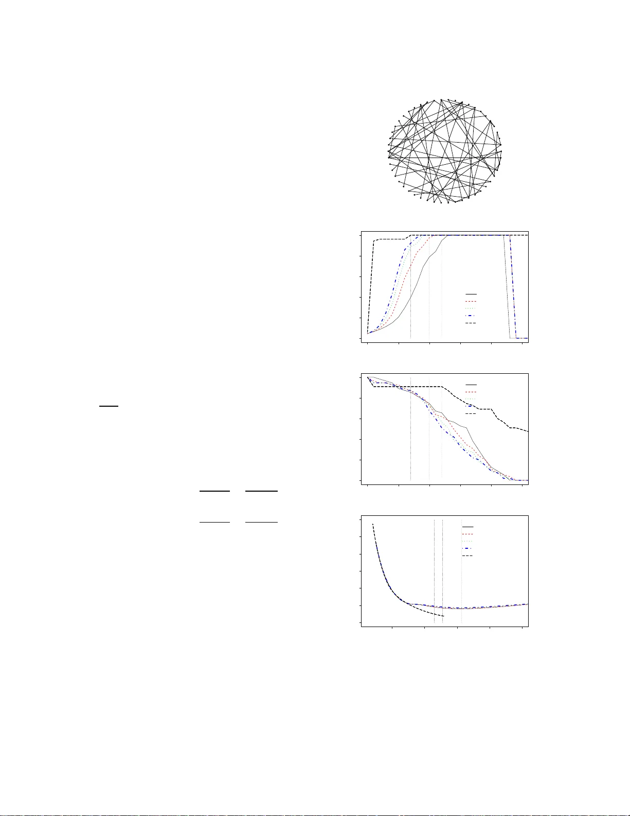
Time V arying Undir ected Graphs Shuheng Zhou, John Lafferty and Larry W asserman ∗ Carnegie Mellon Uni versity { szhou, lafferty } @c s.cmu.edu, larry@stat.cmu.edu Abstract Undirected graphs are often used to describe high dimensiona l distrib ution s. Under spar- sity condition s, the graph can be estimated us- ing ℓ 1 penalization methods. Howe ver , cur- rent method s assume that the data are inde- penden t and identically distributed. If the dis- tribution, and hence the graph, ev olves over time then the data ar e no t longer identically distributed. I n this paper, we sho w how to es- timate the sequen ce of graphs for non-iden tically distributed data, where the distribution e volves over time. 1 Intr oduction Let Z = ( Z 1 , . . . , Z p ) T be a r andom vector with dis- tribution P . The d istribution can be re presented b y an undirected graph G = ( V , F ) . Th e vertex set V h as one vertex for each component of the vector Z . The edge set F con sists of pairs ( j, k ) that ar e join ed by an edge. If Z j is indep endent o f Z k giv en the o ther variables, then ( j, k ) is not in F . When Z is Gau ssian, missing edge s correspo nd to ze roes in the inverse cov arian ce matrix Σ − 1 . Suppose we hav e indepen dent, iden tically dis- tributed data D = ( Z 1 , . . . , Z t , . . . , Z n ) from P . When p is sm all, the grap h m ay be estimated fro m D by test- ing which partial co rrelations are not significantly d iffer - ent f rom zer o [DP04]. When p is large, estimating G is much more dif ficult. Howe ver , if the graph is sparse an d the data are Gaussian, the n several methods can su ccess- fully estimate G ; see [MB06, BGd0 8, FHT07, LF07, BL08, RBLZ07]. All these me thods assume th at the g raphica l stru c- ture is stable over time. But it is e asy to ima gine cases where such stability would fail. For example, Z t could ∗ This research was supported in part by NSF grant CCF - 062587 9. SZ thanks Alan Frieze and Giova nni Leoni for helpful discussions on sparsity and smoothness of functions. W e thank J. Friedman, T . Hastie and R. Tibshirani for mak- ing GLASSO publicly av ailable, an d anon ymous re vie wers for their constructi ve comments. represent a large vector of stock prices at time t . The condition al indep endence structure between stocks could easily change over time. Ano ther examp le is ge ne ex- pression lev els. As a cell m oves thro ugh its m etabolic cycle, the cond itional indepen dence relations between proteins could change. In this pap er we dev elop a nonpar ametric meth od for estimating time varying graphical structur e for m ul- ti variate Gaussian distributions using ℓ 1 regularization method. W e show th at, as lon g as the covariances change smoothly o ver time, we can esti mate the cov ariance ma- trix well (in pr edictive risk) even when p is large. W e make the following theo retical contributions: ( i) non- parametric pred icti ve r isk consistency and rate o f con- vergence o f the cov arian ce m atrices, (ii) consistency and rate of co n vergence in Fro benius n orm of th e inv erse covariance matrix, (iii) large deviation results for co - variance matrices for no n-identica lly distributed obser- vations, and (iv) con ditions that g uarantee smoo thness of th e c ovariances. In addition , we provide simulation evidence tha t we can recover graph ical stru cture. W e believe these are the first such results o n time varying undirected graphs. 2 The Model and Method Let Z t ∼ N (0 , Σ( t )) be indepe ndent. It will be useful to in dex time as t = 0 , 1 /n, 2 /n, . . . , 1 and thus the data are D n = ( Z t : t = 0 , 1 /n, . . . , 1) . Associated with each each Z t is its u ndirected graph G ( t ) . Under the assumption that the la w L ( Z t ) of Z t changes smoothly , we e stimate th e graph sequen ce G (1) , G (2) , . . . , . The graph G ( t ) is d etermined by the zeroes of Σ( t ) − 1 . This method ca n be used to in vestigate a simp le time series model of the form: W 0 ∼ N (0 , Σ(0 )) , an d W t = W t − 1 + Z t , where Z t ∼ N (0 , Σ( t )) . Ultimately , we are interested in the genera l tim e series model where the Z t ’ s ar e dependen t and the gr aphs change over tim e. For simplicity , ho wever , we assume inde pen- dence but allow the g raphs to ch ange. Indeed, it is the changin g graph , ra ther th an th e depend ence, tha t is the biggest hurd le to deal with. In the iid case, re cent work [BGd 08, FHT07] has considered ℓ 1 -penalized maxim um likelihoo d estima tors over the entire set of positive definite matrices, b Σ n = arg min Σ ≻ 0  tr(Σ − 1 b S n ) + log | Σ | + λ | Σ − 1 | 1  (1) where b S n is the sample covariance matrix . In the n on-iid case our approac h is to estimate Σ( t ) at time t by b Σ n ( t ) = ar g min Σ ≻ 0  tr(Σ − 1 b S n ( t )) + log | Σ | + λ | Σ − 1 | 1  where b S n ( t ) = P s w st Z s Z T s P s w st (2) is a weigh ted covariance matrix, with weigh ts w st = K  | s − t | h n  giv en b y a symmetric nonn egati ve fun ction kernel over tim e; in oth er words, b S n ( t ) is ju st the ker- nel estimator of the covariance at time t . An a ttraction of this appro ach is that it can use existing so ftware f or covariance e stimation in the iid setting. 2.1 Notatio n W e use the following notation througho ut the rest of the paper . For any ma trix W = ( w ij ) , let | W | den ote the determinan t of W , tr( W ) the trace of W . Let ϕ max ( W ) and ϕ min ( W ) be the largest and smallest eigenv alues, respectively . W e write W ց = diag ( W ) for a diagon al matrix with th e same d iagonal as W , and W ♦ = W − W ց . The m atrix Frob enius norm is given by k W k F = q P i P j w 2 ij . The oper ator norm k W k 2 2 is given by ϕ max ( W W T ) . W e write | · | 1 for the ℓ 1 norm of a m a- trix vectoriz ed, i.e. , for a matrix | W | 1 = k vec W k 1 = P i P j | w ij | , an d write k W k 0 for the n umber of no n- zero entries in the matrix. W e use Θ( t ) = Σ − 1 ( t ) . 3 Risk Consistency In th is section we define the loss and risk. Consider es- timates b Σ n ( t ) an d b G n ( t ) = ( V , b F n ) . The first risk func- tion is U ( G ( t ) , b G n ( t )) = E L ( G ( t ) , b G n ( t )) (3) where L ( G ( t ) , b G n ( t )) =    F ( t ) ∆ b F n ( t )    , th at is, the size of the symmetric dif feren ce between two edge sets. W e s ay that b G n ( t ) is sparsistent if U ( G ( t ) , b G n ( t )) P → 0 as n → ∞ . The second risk is defined as follows. Let Z ∼ N (0 , Σ 0 ) and let Σ be a positive d efinite matrix. Let R (Σ) = tr(Σ − 1 Σ 0 ) + log | Σ | . (4) Note that, up to an additive co nstant, R (Σ) = − 2 E 0 (log f Σ ( Z )) , where f Σ is the density for N (0 , Σ) . W e say that b G n ( t ) is persistent [GR04] with respe ct to a class of positive definite matrices S n if R ( b Σ n ) − min Σ ∈S n R (Σ) P → 0 . In the iid case, ℓ 1 regularization yields a per sistent esti- mator, as we now show . The maximum likelihood estimate minimizes b R n (Σ) = tr(Σ − 1 b S n ) + log | Σ | , where b S n is the sample covariance matrix . Minimizing b R n (Σ) without constrain ts g iv es b Σ n = b S n . W e would like to minimize b R n (Σ) subject to k Σ − 1 k 0 ≤ L. This would give th e “ best” sparse gra ph G , but it is n ot a conv ex op timization problem. Hence we estima te b Σ n by solving a conv ex relaxation problem as written in (1) instead. Algorithms fo r carr ying out this op timization are giv en by [BGd08, FHT07]. Given L n , ∀ n , let S n = { Σ : Σ ≻ 0 ,   Σ − 1   1 ≤ L n } . (5) W e define the oracle estimator and write (1) as (7) Σ ∗ ( n ) = arg min Σ ∈S n R (Σ) , (6) b Σ n = arg min Σ ∈ S n b R n (Σ) . (7) Note that o ne can choo se to on ly pe nalize o ff-diagonal elements o f Σ − 1 as in [RBLZ07], if desired . W e have the following result, who se p roof app ears in Section 3.2. Theorem 1 Suppo se that p n ≤ n ξ for some ξ ≥ 0 and L n = o  n log p n  1 / 2 for (5). Th en for the seq uence of empirical estimators as define d in (7) and Σ ∗ ( n ) , ∀ n as in (6) , R ( b Σ n ) − R (Σ ∗ ( n )) P → 0 . 3.1 Risk Consistency for the Non-identical Case In th e non-iid case we estimate Σ( t ) at time t ∈ [0 , 1] . Giv en Σ( t ) , let b R n (Σ( t )) = tr(Σ( t ) − 1 b S n ( t )) + lo g | Σ( t ) | . For a given ℓ 1 bound L n , we defin e b Σ n ( t ) as the m ini- mizer of b R n (Σ) subject to Σ ∈ S n , b Σ n ( t ) = arg min Σ ∈S n  tr(Σ − 1 b S n ( t )) + log | Σ |  (8) where b S n ( t ) is gi ven in (2), with K ( · ) a symmetric non- negativ e function with compact support: A 1 The kernel fun ction K has a boun ded sup port [ − 1 , 1 ] . Lemma 2 Let Σ( t ) = [ σ j k ( t )] . Suppo se the fo llowing condition s hold: 1. Th er e exist s C 0 > 0 , C such tha t max j,k sup t | σ ′ j k ( t ) | ≤ C 0 and max j,k sup t | σ ′′ j k ( t ) | ≤ C . 2. p n ≤ n ξ for some ξ ≥ 0 . 3. h n ≍ n − 1 / 3 . Then max j,k | b S n ( t, j, k ) − Σ( t, j, k ) | = O P  √ log n n 1 / 3  for all t > 0 . Proof: By the trian gle inequality , | b S n ( t, j, k ) − Σ( t, j, k ) | ≤ | b S n ( t, j, k ) − E b S n ( t, j, k ) | + | E b S n ( t, j, k ) − Σ( t, j, k ) | . In Lemma 14 we show that max j,k sup t | E b S n ( t, j, k ) − Σ( t, j, k ) | = O ( C 0 h n ) . In Lemma 15, we show that P  | b S n ( t, j, k ) − E b S n ( t, j, k )) | > ǫ  ≤ ex p  − c 1 h n nǫ 2  for some c 1 > 0 . Hence, P  max j,k | b S n ( t, j, k ) − E b S n ( t, j, k ) | > ǫ  ≤ exp  − nh n ( C ǫ 2 − 2 ξ log n / ( nh n ))  and (9) max j,k | b S n ( t, j, k ) − E b S n ( t, j, k ) | = O P  q log n nh n  . Hence the result holds for h n ≍ n − 1 / 3 .  W ith the u se of Lemma 2, the proof of the following follows the s ame lines as th at of Theorem 1. Theorem 3 Suppo se all conditions i n Lemma 2 and the following hold: L n = o  n 1 / 3 / p log n  . (10) Then, ∀ t > 0 , for the sequence of estimators as in (8), R ( b Σ n ( t )) − R (Σ ∗ ( t )) P → 0 . Remark 4 If a local linear smooth er is substituted for a kernel smoother , the rate ca n be impr oved fr om n 1 / 3 to n 2 / 5 as the bias will be boun ded as O ( h 2 ) in (3.1) . Remark 5 Su ppose th at ∀ i, j , if θ ij 6 = 0 , we have θ ij = Ω(1) . Then Condition (10) allows that | Θ | 1 = L n ; hence if p = n ξ and ξ < 1 / 3 , we ha ve tha t k Θ k 0 = Ω( p ) . Hen ce the fa mily of graphs th at we can guaran- tee persistency for , althoug h sparse, is likely to include connected graphs, fo r example, when Ω( p ) ed ges wer e formed randomly among p no des. The smo othness con dition in Lemma 2 is expressed in terms of the elements of Σ( t ) = [ σ ij ( t )] . It might be more na tural to impose smoothn ess o n Θ( t ) = Σ( t ) − 1 instead. In fact, smoo thness of Θ t implies smoo thness of Σ t as th e next result shows. L et us first sp ecify two assumptions. W e u se σ 2 i ( x ) as a shorth and for σ ii ( x ) . Definition 6 F or a fun ction u : [0 , 1 ] → R , let k u k ∞ = sup x ∈ [0 , 1] | u ( x ) | . A 2 There exists some constant S 0 < ∞ su ch that max i =1 ...,p sup t ∈ [0 , 1] | σ i ( t ) | ≤ S 0 < ∞ , h ence (11) max i =1 ...,p k σ i k ∞ ≤ S 0 . (12) A 3 Let θ ij ( t ) , ∀ i, j, be twice d iffer en tiable fun ctions such that θ ′ ij ( t ) < ∞ and θ ′′ ij ( t ) < ∞ , ∀ t ∈ [0 , 1] . In add i- tion, ther e exist constants S 1 , S 2 < ∞ such that sup t ∈ [0 , 1] p X k =1 p X ℓ =1 p X i =1 p X j =1 | θ ′ ki ( t ) θ ′ ℓj ( t ) | ≤ S 1 (13) sup t ∈ [0 , 1] p X k =1 p X ℓ =1 | θ ′′ kℓ ( t ) | ≤ S 2 , (14) wher e the first inequality guarantees that sup t ∈ [0 , 1] P p k =1 P p ℓ =1 | θ ′ kℓ ( t ) | < √ S 1 < ∞ . Lemma 7 Den ote the elements of Θ( t ) = Σ( t ) − 1 by θ j k ( t ) . Under A 2 a nd A 3, th e smoothn ess condition in Lemma 2 holds. The p roof is in Section 6 . In Sectio n 7, we show some preliminar y results on achieving u pper bounds on quan- tities that appear in Cond ition 1 of Lemma 2 throu gh the spar sity level of the in verse covariance matrix, i.e., k Θ t k 0 , ∀ t ∈ [0 , 1] . 3.2 Proof of Th eorem 1 Note that ∀ n , sup Σ ∈S n | R (Σ) − b R n (Σ) | ≤ X j,k | Σ − 1 j k | | b S n ( j, k ) − Σ 0 ( j, k ) | ≤ δ n   Σ − 1   1 , where it follows from [RBLZ07] that δ n = max j,k | b S n ( j, k ) − Σ 0 ( j, k ) | = O P ( p log p/n ) . Hence, m inimizing over S n with L n = o  n log p n  1 / 2 , sup Σ ∈S n | R (Σ) − b R n (Σ) | = o P (1) . By the definitions of Σ ∗ ( n ) ∈ S n and b Σ n ∈ S n , we im mediately have R (Σ ∗ ( n )) ≤ R ( b Σ n ) and b R n ( b Σ n ) ≤ b R n (Σ ∗ ( n )) ; thus 0 ≤ R ( b Σ n ) − R (Σ ∗ ( n )) = R ( b Σ n ) − b R n ( b Σ n ) + b R n ( b Σ n ) − R (Σ ∗ ( n )) ≤ R ( b Σ n ) − b R n ( b Σ n ) + b R n (Σ ∗ ( n )) − R (Σ ∗ ( n )) Using the triangle inequality and b Σ n , Σ ∗ ( n ) ∈ S n , | R ( b Σ n ) − R (Σ ∗ ( n )) | ≤ | R ( b Σ n ) − b R n ( b Σ n ) + b R n (Σ ∗ ( n )) − R (Σ ∗ ( n )) | ≤ | R ( b Σ n ) − b R n ( b Σ n ) | + | b R n (Σ ∗ ( n )) − R (Σ ∗ ( n )) | ≤ 2 sup Σ ∈S n | R (Σ) − b R n (Σ) | . Thu s ∀ ǫ > 0 , the event n    R ( b Σ n ) − R (Σ ∗ ( n ))    > ǫ o is con tained in the event n sup Σ ∈S n | R (Σ) − b R n (Σ) | > ǫ/ 2 o . Thu s, for L n = o (( n/ log n ) 1 / 2 ) , and ∀ ǫ > 0 , as n → ∞ , P     R ( b Σ n ) − R (Σ ∗ ( n ))    > ǫ  ≤ P  sup Σ ∈S n | R (Σ) − b R n (Σ) | > ǫ/ 2  → 0 .  4 Fr obenius No rm Consistency In this section, we sh ow an explicit conver gen ce r ate in the Frobenius nor m for estima ting Θ( t ) , ∀ t , wh ere p, | F | gr ow with n , so lon g as th e covariances chan ge smoothly over t . No te that c ertain smoothn ess assump- tions on a m atrix W would guarantee th e correspondin g smoothne ss con ditions on its in verse W − 1 , so lo ng as W is non-sin gular, as we show in Section 6. W e fir st write our time-varying estimator b Θ n ( t ) for Σ − 1 ( t ) at time t ∈ [0 , 1 ] as the m inimizer of the ℓ 1 regularized negativ e smoothed log- likelihood over the entire set of positive d efinite matrices, b Θ n ( t ) = ar g min Θ ≻ 0  tr(Θ b S n ( t )) − log | Θ | + λ n | Θ | 1  (15) where λ n is a non -negative r egularization p arameter, and b S n ( t ) is the smoothed sample cov arian ce m atrix using a kernel function as defined in (2). Now fix a poin t of interest t 0 . In the following, we use Σ 0 = ( σ ij ( t 0 )) to denote the true covariance matrix at this time. Let Θ 0 = Σ − 1 0 be its in verse matrix. Define the set S = { ( i, j ) : θ ij ( t 0 ) 6 = 0 , i 6 = j } . Then | S | = s . Note that | S | is twice the n umber of edg es in the gr aph G ( t 0 ) . W e make the following assum ptions. A 4 Let p + s = o  n (2 / 3) / lo g n  and ϕ min (Σ 0 ) ≥ k > 0 , h ence ϕ max (Θ 0 ) ≤ 1 /k . F or som e sufficiently large constant M , let ϕ min (Θ 0 ) = Ω  2 M q ( p + s ) log n n 2 / 3  . The proof draws upon techniqu es from [RBLZ07 ], with modification s necessary to handle the fact that we pe- nalize | Θ | 1 rather than | Θ ♦ | 1 as in their case. Theorem 8 Let b Θ n ( t ) be the minimizer define d by (15) . Suppo se all cond itions in Lemma 2 and A 4 hold. If λ n ≍ r log n n 2 / 3 , then k b Θ n ( t ) − Θ 0 k F = O P 2 M r ( p + s ) log n n 2 / 3 ! . ( 16) Proof: Let 0 be a matrix with all entries being zero. Let Q (Θ) = tr(Θ b S n ( t 0 )) − log | Θ | + λ | Θ | − tr(Θ 0 b S n ( t 0 )) + log | Θ 0 | − λ | Θ 0 | 1 = tr  (Θ − Θ 0 )( b S n ( t ) − Σ 0 )  − (log | Θ | − log | Θ 0 | ) + tr ((Θ − Θ 0 )Σ 0 ) + λ ( | Θ | 1 − | Θ 0 | 1 ) . (17) b Θ minimizes Q (Θ) , or equi valently b ∆ n = b Θ − Θ 0 min- imizes G (∆) ≡ Q (Θ 0 + ∆) . Hence G (0 ) = 0 an d G ( b Θ n ) ≤ G (0) = 0 by defin ition. Define f or some constant C 1 , δ n = C 1 q log n n 2 / 3 . Now , let λ n = C 1 ε r log n n 2 / 3 = δ n ε for some 0 < ε < 1 . (18) Consider now the set T n = { ∆ : ∆ = B − Θ 0 , B , Θ 0 ≻ 0 , k ∆ k F = M r n } , where r n = r ( p + s ) lo g n n 2 / 3 ≍ δ n √ p + s → 0 . (19) Claim 9 Un der A 4, for all ∆ ∈ T n such that k ∆ k F = o (1) as in (19) , Θ 0 + v ∆ ≻ 0 , ∀ v ∈ I ⊃ [0 , 1] . Proof: It is sufficient to sh ow that Θ 0 + (1 + ε )∆ ≻ 0 and Θ 0 − ε ∆ ≻ 0 fo r some 1 > ε > 0 . Indeed, ϕ min (Θ 0 + (1 + ε )∆) ≥ ϕ min (Θ 0 ) − (1 + ε ) k ∆ k 2 > 0 for ε < 1 , given that ϕ min (Θ 0 ) = Ω(2 M r n ) and k ∆ k 2 ≤ k ∆ k F = M r n . Similarly , ϕ min (Θ 0 − ε ∆) ≥ ϕ min (Θ 0 ) − ε k ∆ k 2 > 0 for ε < 1 .  Thus we have th at lo g det(Θ 0 + v ∆) is infinitely differentiable on the o pen interval I ⊃ [0 , 1] of v . This allows us to use th e T aylor’ s for mula with integra l re- mainder to obtain the following lemma: Lemma 10 W ith pr oba bility 1 − 1 /n c for some c ≥ 2 , G (∆) > 0 for all ∆ ∈ T n . Proof: Let u s use A as a shorthand for vec ∆ T  Z 1 0 (1 − v )(Θ 0 + v ∆) − 1 ⊗ (Θ 0 + v ∆) − 1 dv  vec∆ , where ⊗ is the Kr onecker prod uct ( if W = ( w ij ) m × n , P = ( b kℓ ) p × q , then W ⊗ P = ( w ij P ) mp × nq ), and vec ∆ ∈ R p 2 is ∆ p × p vectorized. Now , the T a ylor ex- pansion giv es log | Θ 0 + ∆ | − lo g | Θ 0 | = d dv log | Θ 0 + v ∆ || v =0 ∆ + R 1 0 (1 − v ) d 2 dv 2 log det(Θ 0 + v ∆) dv = tr(Σ 0 ∆) + A, where by symmetry , tr (Σ 0 ∆) = tr(Θ − Θ 0 )Σ 0 . Hence G (∆) = (20) A + tr  ∆( b S n − Σ 0 )  + λ n ( | Θ 0 + ∆ | 1 − | Θ 0 | 1 ) . For an index set S and a matrix W = [ w ij ] , write W S ≡ ( w ij I (( i, j ) ∈ S )) , where I ( · ) is an indicato r fu nction. Recall S = { ( i, j ) : Θ 0 ij 6 = 0 , i 6 = j } and let S c = { ( i, j ) : Θ 0 ij = 0 , i 6 = j } . Hence Θ = Θ ց + Θ ♦ S + Θ ♦ S c , ∀ Θ in our no tation. Note that we have Θ ♦ 0 S c = 0 , | Θ ♦ 0 + ∆ ♦ | 1 = | Θ ♦ 0 S + ∆ ♦ S | 1 + | ∆ ♦ S c | 1 , | Θ ♦ 0 | 1 = | Θ ♦ 0 S | 1 , hence | Θ ♦ 0 + ∆ ♦ | 1 − | Θ ♦ 0 | 1 ≥   ∆ ♦ S c   1 −   ∆ ♦ S   1 , | Θ ց 0 + ∆ ց | 1 − | Θ ց 0 | 1 ≥ −| ∆ ց | 1 , where the last two steps follow from the trian gle in- equality . Th erefore | Θ 0 + ∆ | 1 − | Θ 0 | 1 = | Θ ♦ 0 + ∆ ♦ | 1 − | Θ ♦ 0 | 1 + | Θ ց 0 + ∆ ց | 1 − | Θ ց 0 | 1 ≥   ∆ ♦ S c   1 −   ∆ ♦ S   1 − | ∆ ց | 1 . (21) Now , from Lemma 2, max j,k | b S n ( t, j, k ) − σ ( t, j, k ) | = O P  √ log n n 1 / 3  = O P ( δ n ) . By ( 9), with proba bility 1 − 1 n 2    tr  ∆( b S n − Σ 0 )     ≤ δ n | ∆ | 1 , hence by (21) tr  ∆( b S n − Σ 0 )  + λ n ( | Θ 0 + ∆ | 1 − | Θ 0 | 1 ) ≥ − δ n | ∆ ց | 1 − δ n   ∆ ♦ S c   1 − δ n   ∆ ♦ S   1 − λ n | ∆ ց | 1 + λ n   ∆ ♦ S c   1 − λ n   ∆ ♦ S   1 ≥ − ( δ n + λ n )  | ∆ ց | 1 +   ∆ ♦ S   1  + ( λ n − δ n )   ∆ ♦ S c   1 ≥ − ( δ n + λ n )  | ∆ ց | 1 +   ∆ ♦ S   1  , wh ere (22) ( δ n + λ n )  | ∆ ց | 1 +   ∆ ♦ S   1  ≤ ( δ n + λ n )  √ p k ∆ ց k F + √ s k ∆ ♦ S k F  ≤ ( δ n + λ n )  √ p k ∆ ց k F + √ s k ∆ ♦ k F  ≤ ( δ n + λ n ) max { √ p, √ s }  k ∆ ց k F + k ∆ ♦ k F  ≤ ( δ n + λ n ) max { √ p, √ s } √ 2 k ∆ k F ≤ δ n 1 + ε ε √ p + s √ 2 k ∆ k F . (23) Combining (2 0), (22), and ( 23), we have with prob abil- ity 1 − 1 n c , for all ∆ ∈ T n , G (∆) ≥ A − ( δ n + λ n )  | ∆ ց | 1 +   ∆ ♦ S   1  ≥ k 2 2 + τ k ∆ k 2 F − δ n 1 + ε ε √ p + s √ 2 k ∆ k F = k ∆ k 2 F k 2 2 + τ − δ n √ 2(1 + ε ) ε k ∆ k F √ p + s ! = k ∆ k 2 F k 2 2 + τ − δ n √ 2(1 + ε ) εM r n √ p + s ! > 0 for M sufficiently large, wh ere the b ound on A co mes from Lemma 11 by [RBLZ07].  Lemma 11 ( [RBLZ07]) F or some τ = o (1) , und er A 4, vec ∆ T  R 1 0 (1 − v )(Θ 0 + v ∆) − 1 ⊗ (Θ 0 + v ∆) − 1 dv  vec ∆ ≥ k ∆ k 2 F k 2 2+ τ , for all ∆ ∈ T n . W e next show the follo wing claim. Claim 12 If G (∆) > 0 , ∀ ∆ ∈ T n , then G (∆) > 0 fo r all ∆ in V n = { ∆ : ∆ = D − Θ 0 , D ≻ 0 , k ∆ k F > M r n , for r n as in (19) } . Hence if G (∆) > 0 , ∀ ∆ ∈ T n , then G (∆) > 0 for all ∆ ∈ T n ∪ V n . Proof: Now by con tradiction , supp ose G (∆ ′ ) ≤ 0 f or some ∆ ′ ∈ V n . Let ∆ 0 = M r n k ∆ ′ k F ∆ ′ . Thus ∆ 0 = θ 0 + (1 − θ )∆ ′ , where 0 < 1 − θ = M r n k ∆ ′ k F < 1 b y definition of ∆ 0 . Hence ∆ 0 ∈ T n giv en th at Θ 0 + ∆ 0 ≻ 0 by Claim 1 3. Hence by conve xity of G (∆) , we h av e that G (∆ 0 ) ≤ θ G (0 ) + (1 − θ ) G (∆ ′ ) ≤ 0 , con tradicting that G (∆ 0 ) > 0 for ∆ 0 ∈ T n .  By Claim 12 an d th e fact that G ( b ∆ n ) ≤ G (0) = 0 , we have the following: If G (∆) > 0 , ∀ ∆ ∈ T n , then b ∆ n 6∈ ( T n ∪ V n ) , that is, k b ∆ n k F < M r n , g iv en that b ∆ n = b Θ n − Θ 0 , where b Θ n , Θ 0 ≻ 0 . Therefo re P  k b ∆ n k F ≥ M r n  = 1 − P  k b ∆ n k F < M r n  ≤ 1 − P ( G (∆) > 0 , ∀ ∆ ∈ T n ) = P ( G (∆) ≤ 0 for some ∆ ∈ T n ) < 1 n c . W e thu s establish that k b ∆ n k F ≤ O P ( M r n ) .  Claim 13 Let B be a p × p matrix. If B ≻ 0 and B + D ≻ 0 , then B + v D ≻ 0 for all v ∈ [0 , 1] . Proof: W e on ly need to check for v ∈ (0 , 1 ) , where 1 − v > 0 ; ∀ x ∈ R p , by B ≻ 0 and B + D ≻ 0 , x T B x > 0 and x T ( B + D ) x > 0 ; h ence x T D x > − x T B x . Th us x T ( B + v D ) x = x T B x + v x T D x > (1 − v ) x T B x > 0 .  5 Large Deviation Ine qualities Before we go on, we explain the notation that w e fol- low throug hout this sectio n. W e switch notatio n fro m t to x a nd f orm a regression problem for non -iid d ata. Giv en an interval of [0 , 1] , the p oint of interest is x 0 = 1 . W e for m a design matrix by samp ling a set of n p - dimensiona l Gaussian random vectors Z t at t = 0 , 1 /n, 2 /n, . . . , 1 , where Z t ∼ N (0 , Σ t ) are indep endently distributed. In this sectio n, we in dex the rando m vectors Z with k = 0 , 1 , . . . , n such that Z k = Z t for k = nt , with cor respond ing covariance m atrix deno ted by Σ k . Hence Z k = ( Z k 1 , . . . , Z kp ) T ∼ N (0 , Σ k ) , ∀ k . (24) These are indepen dent but no t iden tically distributed. W e will need to gen eralize the u sual inequ alities. In Section A, v ia a boxcar k ern el function , we use moment generating function s to show that for b Σ = 1 n P n k =1 Z k Z T k , P n ( | b Σ ij − Σ ij ( x 0 ) | > ǫ ) < e − cnǫ 2 (25) where P n = P 1 × · · · × P n denotes th e p roduc t measure. W e loo k across n time-varying Gaussian vectors, and rough ly , we compar e b Σ ij with Σ ij ( x 0 ) , where Σ( x 0 ) = Σ n is the covariance m atrix in the end of th e win dow for t 0 = n . Furtherm ore, we derive inequalities in Sec- tion 5.1 for a genera l k ern el function. 5.1 Bounds For K ernel Smoothing In this section, we derive large deviation ineq ualities for the covariance matrix b ased on kern el regression estima- tions. Recall t ha t we assume th at the symmetric no nneg- ativ e kern el func tion K has a b ound ed support [ − 1 , 1 ] in A 1. This kernel has the property that: 2 Z 0 − 1 v K ( v ) dv ≤ 2 Z 0 − 1 K ( v ) dv = 1 (2 6) 2 Z 0 − 1 v 2 K ( v ) dv ≤ 1 . (27) In orde r to estimate t 0 , instead of taking an average of sample variances/covariances over the last n samples, we use the weighting scheme such th at data close to t 0 receives larger weights than those that are far away . Let Σ( x ) = ( σ ij ( x )) . Let us define x 0 = t 0 n = 1 , and ∀ i = 1 , . . . , n , x i = t 0 − i n and ℓ i ( x 0 ) = 2 nh K  x i − x 0 h  ≈ K  x i − x 0 h  P n i =1 K  x i − x 0 h  (28) where th e ap prox imation is due to rep lacing the sum with the Riemann integral: n X i =1 ℓ i ( x 0 ) = n X i =1 2 nh K  x i − x 0 h  ≈ 2 Z 0 − 1 K ( v ) dv = 1 , due to the fact that K ( v ) has compact suppor t in [ − 1 , 1] and h ≤ 1 . L et Σ k = ( σ ij ( x k )) , ∀ k = 1 , . . . , n, where σ ij ( x k ) = c ov ( Z ki , Z kj ) = ρ ij ( x k ) σ i ( x k ) σ j ( x k ) an d ρ ij ( x k ) is the correlatio n coefficient between Z i and Z j at time x k . Recall tha t w e h ave indepen dent ( Z ki Z kj ) for all k = 1 , . . . , n such th at E ( Z ki Z kj ) = σ ij ( x k ) . Let Φ 1 ( i, j ) = 1 n n X k =1 2 h K  x k − x 0 h  σ ij ( x k ) , hence E n X k =1 ℓ k ( x 0 ) Z ki Z kj = n X k =1 ℓ k ( x 0 ) σ ij ( x k ) = Φ 1 ( i, j ) . W e thu s decompose and bound for point of interest x 0      n X k =1 ℓ k ( x 0 ) Z ki Z kj − σ ij ( x 0 )      ≤      E n X k =1 ℓ k ( x 0 ) Z ki Z kj − σ ij ( x 0 )      +      n X k =1 ℓ k ( x 0 ) Z ki Z kj − E n X k =1 ℓ k ( x 0 ) Z ki Z kj      (29) =      n X k =1 ℓ k ( x 0 ) Z ki Z kj − Φ 1 ( i, j )      + | Φ 1 ( i, j ) − σ ij ( x 0 ) | . Before we start our analysis on large deviations, we first look at the bias term. Lemma 14 Su ppose ther e exis ts C > 0 such that max i,j sup t | σ ′′ ( t, i, j ) | ≤ C. Then ∀ t ∈ [0 , 1 ] , max i,j | E b S n ( t, i, j ) − σ ij ( t ) | = O ( h ) . Proof: W .l.o .g, let t = t 0 , h ence E b S n ( t, i, j ) = Φ 1 ( i, j ) . W e use th e Riemann integral to approximate the s um , Φ 1 ( i, j ) = 1 n n X k =1 2 h K  x k − x 0 h  σ ij ( x k ) ≈ Z x 0 x n 2 h K  u − x 0 h  σ ij ( u ) du = 2 Z 0 − 1 /h K ( v ) σ ij ( x 0 + hv ) dv . W e n ow use T aylo r’ s Formu la to rep lace σ ij ( x 0 + hv ) and obtain 2 R 0 − 1 /h K ( v ) σ ij ( x 0 + hv ) dv = 2 R 0 − 1 K ( v )  σ ij ( x 0 ) + hv σ ′ ij ( x 0 ) + σ ′′ ij ( y ( v ))( hv ) 2 2  dv = σ ij ( x 0 ) + 2 R 0 − 1 K ( v )  hv σ ′ ij ( x 0 ) + C ( hv ) 2 2  dv , where 2 Z 0 − 1 K ( v )  hv σ ′ ij ( x 0 ) + C ( hv ) 2 2  dv = 2 hσ ′ ij ( x 0 ) Z 0 − 1 v K ( v ) dv + C h 2 2 Z 0 − 1 v 2 K ( v ) dv ≤ hσ ′ ij ( x 0 ) + C h 2 4 , where y ( v ) − x 0 < hv . Thus Φ 1 ( i, j ) − σ ij ( x 0 ) = O ( h ) .  W e now move on to the large deviation boun d fo r all entries of the smoothed empirical covariance m atrix. Lemma 15 F or ǫ < C 1 ( σ 2 i ( x 0 ) σ 2 j ( x 0 )+ σ 2 ij ( x 0 ) ) max k =1 ,...,n “ 2 K “ x k − x 0 h ” σ i ( x k ) σ j ( x k ) ” , wher e C 1 is defined in Claim 18, for some C > 0 , P  | b S n ( t, i, j ) − E b S n ( t, i, j ) | > ǫ  ≤ exp  − C nhǫ 2  . Proof: Let u s define A k = Z ki Z kj − σ ij ( x k ) . P  | b S n ( t, i, j ) − E b S n ( t, i, j ) | > ǫ  = P n X k =1 ℓ k ( x 0 ) Z ki Z kj − n X k =1 ℓ k ( x 0 ) σ ij ( x k ) > ǫ ! For e very t > 0 , we h av e by Markov’ s inequality P n X k =1 nℓ k ( x 0 ) A k > nǫ ! = P  e t P n k =1 2 h K ( x i − x 0 h ) A k > e ntǫ  ≤ E e t P n k =1 2 h K ( x i − x 0 h ) A k e ntǫ . (30) Before we continu e, fo r a g iv en t , let us first define the following qu antities, where i, j ar e omitted from Φ 1 ( i, j ) • a k = 2 t h K  x k − x 0 h  ( σ i ( x k ) σ j ( x k ) + σ ij ( x k )) • b k = 2 t h K  x k − x 0 h  ( σ i ( x k ) σ j ( x k ) − σ ij ( x k )) thu s • Φ 1 = 1 n P n k =1 a k − b k 2 t , Φ 2 = 1 n P n k =1 a 2 k + b 2 k 4 t 2 • Φ 3 = 1 n P n k =1 a 3 k − b 3 k 6 t 3 , Φ 4 = 1 n P n k =1 a 4 k + b 4 k 8 t 4 • M = max k =1 ,...,n  2 h K  x k − x 0 h  σ i ( x k ) σ j ( x k )  W e now establish some convenient comparison s; see Sec- tion B.1 and B.2 for their proof s. Claim 16 Φ 3 Φ 2 ≤ 4 M 3 and Φ 4 Φ 2 ≤ 2 M 2 , wher e b oth equal- ities ar e established at ρ ij ( x k ) = 1 , ∀ k . Lemma 17 F or b k ≤ a k ≤ 1 2 , ∀ k , 1 2 P n k =1 ln 1 (1 − a k )(1+ b k ) ≤ nt Φ 1 + nt 2 Φ 2 + nt 3 Φ 3 + 9 5 nt 4 Φ 4 . T o show the f ollowing, we first replace the sum with a Riemann integral, and then use T aylor’ s Formula to ap- proxim ate σ i ( x k ) , σ j ( x k ) , an d σ ij ( x k ) , ∀ k = 1 , . . . , n with σ i , σ j σ ij and th eir first deriv atives at x 0 respec- ti vely , plus some r emainder ter ms; see Sectio n B.3 fo r details. Claim 18 F or h = n − ǫ for some 1 > ǫ > 0 , ther e e xists some constant C 1 > 0 such that Φ 2 ( i, j ) = C 1 ( σ 2 i ( x 0 ) σ 2 j ( x 0 ) + σ 2 ij ( x 0 )) h . Lemma19 comp utes the mom ent generating functio n for 2 h K  x k − x 0 h  Z ki · Z kj . The proo f p roceeds exactly as that o f Lemma 21 after substituting t with 2 t h K  x k − x 0 h  ev ery where. Lemma 19 Let 2 t h K  x k − x 0 h  (1+ ρ ij ( x k )) σ i ( x k ) σ j ( x k ) < 1 , ∀ k . F or b k ≤ a k < 1 . E e 2 t h K “ x k − x 0 h ” Z ki Z kj = ( (1 − a k )(1 + b k )) − 1 / 2 . Remark 20 Th us when we set t = ǫ 4Φ 2 , the bo und on ǫ implies that b k ≤ a k ≤ 1 / 2 , ∀ k : a k = t (1 + ρ ij ( x k )) σ i ( x k ) σ j ( x k ) ≤ 2 tσ i ( x k ) σ j ( x k ) = ǫσ i ( x k ) σ j ( x k ) 2Φ 2 ≤ 1 2 . W e ca n now finish showing the la rge deviation bo und for max i,j | b S i,j − E S i,j | . Given that A 1 , . . . , A n are indepen dent, we have E e t P n k =1 2 h K “ x k − x 0 h ” A k = n Y k =1 E e 2 t h K ( x 1 − x 0 h ) A k = n Y k =1 exp  − 2 t h K  x k − x 0 h  σ ij ( x k )  · n Y k =1 E e 2 t h K “ x k − x 0 h ” Z ki Z kj (31) By (30), (31), Lemma 19, for t ≤ ǫ 4Φ 2 , P n X k =1 2 h K  x k − x 0 h  A k > nǫ ! ≤ E e t P n k =1 2 h K “ x k − x 0 h ” A k e − ntǫ = e − ntǫ · Q n k =1 e − 2 t h K “ x k − x 0 h ” σ ij ( x k ) · E e 2 t h K “ x k − x 0 h ” Z ki Z kj = e − ntǫ − nt Φ 1 ( i,j )+ 1 2 P n k =1 ln 1 (1 − a k )(1+ b k ) ≤ exp  − ntǫ + nt 2 Φ 2 + nt 3 Φ 3 + 9 5 nt 4 Φ 4  , where the last step is due to Remark 20 and Lemm a 17. Now let us consider taking t that minimize s exp  − ntǫ + nt 2 Φ 2 + nt 3 Φ 3 + 9 5 nt 4 Φ 4  ; Let t = ǫ 4Φ 2 : d dt  − ntǫ + nt 2 Φ 2 + nt 3 Φ 3 + 9 5 nt 4 Φ 4  ≤ − ǫ 40 ; Now giv en that ǫ 2 Φ 2 < 1 M , Claim 16 and 18: P n X k =1 2 h K  x k − x 0 h  A k > nǫ ! ≤ exp  − ntǫ + nt 2 Φ 2 + nt 3 Φ 3 + 9 5 nt 4 Φ 4  ≤ exp  − nǫ 2 4Φ 2 + nǫ 2 16Φ 2 + nǫ 2 64Φ 2 ǫ Φ 3 Φ 2 2 + 9 5 nǫ 2 256Φ 2 ǫ 2 Φ 4 Φ 3 2  ≤ exp  − 3 nǫ 2 20Φ 2  ≤ exp − 3 nhǫ 2 20 C 1 ( σ 2 i ( x 0 ) σ 2 j ( x 0 ) + σ 2 ij ( x 0 )) ! . Finally , let’ s check the requirem ent on ǫ ≤ Φ 2 M , ǫ ≤  C 1 (1 + ρ 2 ij ( x 0 )) σ 2 i ( x 0 ) σ 2 j ( x 0 )  /h max k =1 ,...,n  2 h K  x k − x 0 h  σ i ( x k ) σ j ( x k )  =  C 1 (1 + ρ 2 ij ( x 0 )) σ 2 i ( x 0 ) σ 2 j ( x 0 )  max k =1 ,...,n  2 K  x k − x 0 h  σ i ( x k ) σ j ( x k )  .  For completeness, we compute the moment gener at- ing function for Z k,i Z k,j . Lemma 21 Let t (1 + ρ ij ( x k )) σ i ( x k ) σ j ( x k ) < 1 , ∀ k , so that b k ≤ a k < 1 , omitting x k everywher e, E e tZ k,i Z k,j =  1 (1 − t ( σ i σ j + σ ij )(1 + t ( σ i σ j − σ ij ))  1 / 2 . Proof: W .l.o. g., let i = 1 and j = 2 . E  e tZ 1 Z 2  = E  E  e tZ 2 Z 1 | Z 2  = E exp  tρ 12 σ 1 σ 2 + t 2 σ 2 1 (1 − ρ 2 12 ) 2  Z 2 2  =  1 − 2  tρ 12 σ 1 σ 2 + t 2 σ 2 1 (1 − ρ 2 12 ) 2  σ 2 2  − 1 / 2 =  1 1 − (2 tρ 12 σ 1 σ 2 + t 2 σ 2 1 σ 2 2 (1 − ρ 2 12 ))  1 / 2 =  1 (1 − t (1 + ρ 12 ) σ 1 σ 2 )(1 + t (1 − ρ 12 ) σ 1 σ 2 )  1 / 2 where 2 tρ 12 σ 1 σ 2 + t 2 σ 2 1 σ 2 2 (1 − ρ 2 12 ) < 1 . This requires that t < 1 (1+ ρ 12 ) σ 1 σ 2 which is equi valent to 2 tρ 12 σ 1 σ 2 + t 2 σ 2 1 σ 2 2 (1 − ρ 2 12 ) − 1 < 0 . One ca n check that if we require t (1 + ρ 12 ) σ 1 σ 2 ≤ 1 , which im plies th at tσ 1 σ 2 ≤ 1 − tρ 12 σ 1 σ 2 and hence t 2 σ 2 1 σ 2 2 ≤ (1 − tρ 12 σ 1 σ 2 ) 2 , the lemma holds.  6 Smoothness and Sparsity of Σ t via Σ − 1 t In this section we show that if we assume Θ( x ) = ( θ ij ( x )) are smoo th an d twice d ifferentiable functio ns of x ∈ [0 , 1 ] , i.e., θ ′ ij ( x ) < ∞ and θ ′′ ij ( x ) < ∞ for x ∈ [0 , 1] , ∀ i, j , and satisfy A 3, th en the smoothn ess con ditions of Lemma 2 are satisfied. Th e f ollowing is a stan dard r esult in matrix analysis. Lemma 22 Let Θ( t ) ∈ R p × p has entries that a r e dif- fer entiable functions of t ∈ [0 , 1] . Assuming that Θ ( t ) is always non-singu lar , then d dt [Σ( t )] = − Σ( t ) d dt [Θ( t )]Σ( t ) . Lemma 23 Su ppose Θ( t ) ∈ R p × p has entries th at each ar e twice differ e ntiable fun ctions of t . Assumin g tha t Θ( t ) is always non-sing ular , then d 2 dt 2 [Σ( t )] = Σ( t ) D ( t )Σ( t ) , where D ( t ) = 2 d dt [Θ( t )]Σ( t ) d dt [Θ( t )] − d 2 dt 2 [Θ( t )] . Proof: The existence o f the second order de riv ativ es for entries of Σ( t ) is due to the fact that Σ( t ) and d dt [Θ( t )] are both differentiable ∀ t ∈ [0 , 1] ; indeed by Lemma 22, d 2 dt 2 [Σ( t )] = d dt  − Σ( t ) d dt [Θ( t )]Σ( t )  = − d dt [Σ( t )] d dt [Θ( t )]Σ( t ) − Σ( t ) d dt  d dt [Θ( t )]Σ( t )  = − d dt [Σ( t )] d dt [Θ( t )]Σ( t ) − Σ( t ) d 2 dt 2 [Θ( t )]Σ( t ) − Σ( t ) d dt [Θ( t )] d dt [Σ( t )] = Σ( t )  2 d dt [Θ( t )]Σ( t ) d dt [Θ( t )] − d 2 dt 2 [Θ( t )]  Σ( t ) , hence the lemma holds by the definition of D ( t ) .  Let Σ( x ) = ( σ ij ( x )) , ∀ x ∈ [0 , 1] . Let Σ ( x ) = (Σ 1 ( x ) , Σ 2 ( x ) , . . . , Σ p ( x )) , where Σ i ( x ) ∈ R p denotes a column vector . By Lemma 23, σ ′ ij ( x ) = − Σ T i ( x )Θ ′ ( x )Σ j ( x ) , (32) σ ′′ ij ( x ) = Σ T i ( x ) D ( x )Σ j ( x ) , (33) where Θ ′ ( x ) =  θ ′ ij ( x )  , ∀ x ∈ [0 , 1 ] . Lemma 24 Given A 2 an d A 3, ∀ x ∈ [0 , 1 ] , | σ ′ ij ( x ) | ≤ S 2 0 p S 1 < ∞ . Proof: | σ ′ ij ( x ) | = | Σ T i ( x )Θ ′ ( x )Σ j ( x ) | ≤ max i =1 ...,p | σ 2 i ( x ) | p X k =1 p X ℓ =1 | θ ′ kℓ ( x ) | ≤ S 2 0 p S 1 .  W e d enote the elements of Θ( x ) by θ j k ( x ) . Let θ ′ ℓ represent a column vector of Θ ′ . Theorem 25 Given A 2 and A 3, ∀ i, j , ∀ x ∈ [0 , 1] , sup x ∈ [0 , 1]   σ ′′ ij ( x )   < 2 S 3 0 S 1 + S 2 0 S 2 < ∞ . Proof: By (3 3) and the triangle inequality ,   σ ′′ ij ( x )   =   Σ T i ( x ) D ( x )Σ j ( x )   ≤ max i =1 ...,p   σ 2 i ( x )   p X k =1 p X ℓ =1 | D kℓ ( x ) | ≤ S 2 0 p X k =1 p X ℓ =1 2 | θ ′ T k ( x )Σ( x ) θ ′ ℓ ( x ) | + | θ ′′ kℓ ( x ) | = 2 S 3 0 S 1 + S 2 0 S 2 , where by A 3, P p k =1 P p ℓ =1 | θ ′′ kℓ ( x ) | ≤ S 2 , and p X k =1 p X ℓ =1   θ ′ T k ( x )Σ( x ) θ ′ ℓ ( x )   = p X k =1 p X ℓ =1 p X i =1 p X j =1   θ ′ ki ( x ) θ ′ ℓj ( x ) σ ij ( x )   ≤ max i =1 ...,p | σ i ( x ) | p X k =1 p X ℓ =1 p X i =1 p X j =1   θ ′ ki ( x ) θ ′ ℓj ( x )   ≤ S 0 S 1 .  7 Some Implications of a V ery Sparse Θ W e use L 1 to deno te Lebesgu e measure on R . Th e aim of this section is to prove some b ound s that corre spond to A 3, but only for L 1 a.e. x ∈ [0 , 1] , based on a sing le sparsity assum ption on Θ as in A 5. W e let E ⊂ [0 , 1] represent the “bad” set with L 1 ( E ) = 0 . and L 1 a.e. x ∈ [0 , 1 ] r efer to points in the set [0 , 1] \ E such that L 1 ([0 , 1 ] \ E ) = 1 . When k Θ( x ) k 0 ≤ s + p for all x ∈ [0 , 1] , we im mediately obtain T heorem 26, whose proof ap pears in Section 7. 1. W e lik e to poin t out that al- though we apply Theor em 26 to Θ and de duce smooth- ness o f Σ , we co uld a pply it the other way aro und. In particular, it might be interesting to apply it to the cor- relation coefficient matrix ( ρ ij ) , wher e the diagon al en- tries remain inv ariant. W e use Θ ′ ( x ) and Θ ′′ ( x ) to de- note ( θ ′ ij ( x )) and ( θ ′′ ij ( x )) respectively ∀ x . A 5 Assume that k Θ( x ) k 0 ≤ s + p ∀ x ∈ [0 , 1 ] . A 6 ∃ S 4 , S 5 < ∞ such that S 4 = max ij   θ ′ ij   2 ∞ and S 5 = max ij   θ ′′ ij   ∞ . (34) W e state a the orem, the proo f of which is in Section 7.1 and a corollary . Theorem 26 Under A 5, we have k Θ ′′ ( x ) k 0 ≤ k Θ ′ ( x ) k 0 ≤ k Θ( x ) k 0 ≤ s + p for L 1 a.e. x ∈ [0 , 1] . Corollary 27 Given A 2 and A 5, for L 1 a.e. x ∈ [0 , 1] | σ ′ ij ( x ) | ≤ S 2 0 p S 4 ( s + p ) < ∞ . (35) Proof: By pr oof of Lemma 24, | σ ′ ij ( x ) | ≤ max i =1 ...,p k σ 2 i k ∞ P p k =1 P p ℓ =1 | θ ′ kℓ ( x ) | . Hence by Th eorem 26, f or L 1 a.e. x ∈ [0 , 1 ] , | σ ′ ij ( x ) | ≤ max i =1 ...,p k σ 2 i k ∞ P p k =1 P p ℓ =1 | θ ′ kℓ ( x ) | ≤ S 2 0 max k,ℓ k θ ′ kℓ k ∞ k Θ ′ ( x ) k 0 ≤ S 2 0 √ S 4 ( s + p ) .  Lemma 28 Und er A 5 and 6, for L 1 a.e. x ∈ [0 , 1] , p X k =1 p X ℓ =1 p X i =1 p X j =1   θ ′ ki ( x ) θ ′ ℓj ( x )   ≤ ( s + p ) 2 max ij   θ ′ ij   2 ∞ p X k =1 p X ℓ =1 θ ′′ kℓ ≤ ( s + p ) max ij   θ ′′ ij   ∞ , hence ess sup x ∈ [0 , 1] σ ′′ ij ( x ) ≤ 2 S 3 0 ( s + p ) 2 S 4 + S 2 0 ( s + p ) S 5 . Proof: By the trian gle inequality , for L 1 a.e. x ∈ [0 , 1] ,   σ ′′ ij ( x )   =   Σ T i D Σ j   =      p X k =1 p X ℓ =1 σ ik ( x ) σ j ℓ ( x ) D kℓ ( x )      ≤ max i =1 ...,p   σ 2 i   ∞ p X k =1 p X ℓ =1 | D kℓ ( x ) | ≤ 2 S 2 0 p X k =1 p X ℓ =1 | θ ′ T k Σ θ ′ ℓ | + S 2 0 p X k =1 p X ℓ =1 | θ ′′ kℓ | = 2 S 3 0 ( s + p ) 2 S 4 + S 2 0 ( s + p ) S 5 , where for L 1 a.e. x ∈ [0 , 1] , p X k =1 p X ℓ =1   θ ′ T k Σ θ ′ ℓ   ≤ p X k =1 p X ℓ =1 p X i =1 p X j =1   θ ′ ki θ ′ ℓj σ ij   ≤ max i =1 ...,p k σ i k ∞ p X k =1 p X ℓ =1 p X i =1 p X j =1   θ ′ ki θ ′ ℓj   ≤ S 0 ( s + p ) 2 S 4 and P p k =1 P p ℓ =1 | θ ′′ kℓ | ≤ ( s + p ) S 5 . The first ineq ual- ity is due to the follo wing observation: at most ( s + p ) 2 elements in th e sum of P k P i P ℓ P j    θ ′ ki ( x ) θ ′ ℓj ( x )    for L 1 a.e. x ∈ [0 , 1] , that is, except for E , are non- zero, due to the f act that for x ∈ [0 , 1] \ N , k Θ ′ ( x ) k 0 ≤ k Θ( x ) k 0 ≤ s + p as in The orem 26. The second in- equality is obtained similar ly using the fact tha t f or L 1 a.e. x ∈ [0 , 1] , k Θ ′′ ( x ) k 0 ≤ k Θ( x ) k 0 ≤ s + p .  Remark 29 F or the bad set E ⊂ [0 , 1] with L 1 ( E ) = 0 , σ ′ ij ( x ) is well defin ed a s sh own in Lemma 22, but it can on ly be loosely b ounde d by O ( p 2 ) , as k Θ ′ ( x ) k 0 = O ( p 2 ) , instead of s + p , fo r x ∈ E ; similarly , σ ′′ ij ( x ) can only be loosely boun ded by O ( p 4 ) . By Lemma 28, using the Le besgue integral, we can derive th e following corollary . Corollary 30 Under A 2, A 5, and A 6, Z 1 0  σ ′′ ij ( x )  2 dx ≤ 2 S 3 0 S 4 s + p 2 + S 2 0 S 5 ( s + p ) < ∞ . 7.1 Proof of Th eorem 26. Let k Θ( x ) k 0 ≤ s + p fo r all x ∈ [0 , 1] . Lemma 31 Let a func tion u : [0 , 1] → R . Suppo se u has a derivative o n F (fi nite or no t) with L 1 ( u ( F )) = 0 . Then u ′ ( x ) = 0 for L 1 a.e. x ∈ F . T ake F = { x ∈ [0 , 1] : θ ij ( x ) = 0 } an d u = θ ij . For L 1 a.e. x ∈ F , that is, except for a set N ij of L 1 ( N ij ) = 0 , θ ′ ij ( x ) = 0 . Let N = S ij N ij . By Lemma 31, Lemma 32 If x ∈ [0 , 1] \ N , wher e L 1 ( N ) = 0 , if θ ij ( x ) = 0 , then θ ′ ij ( x ) = 0 for all i, j . Let v ij = θ ′ ij . T ake F = { x ∈ [0 , 1] : v ij ( x ) = 0 } . For L 1 a.e. x ∈ F , that is, except for a set N 1 ij with L ( N 1 ij ) = 0 , v ′ ij ( x ) = 0 . Let N 1 = S ij N 1 ij . By Lemma 31, Lemma 33 If x ∈ [0 , 1] \ N 1 , wher e L 1 ( N 1 ) = 0 , if θ ′ ij ( x ) = 0 , then θ ′′ ij ( x ) = 0 , ∀ i, j . Thus this allows t o con clude that Lemma 34 If x ∈ [0 , 1] \ N ∪ N 1 , wher e L 1 ( N ∪ N 1 ) = 0 , if θ ij ( x ) = 0 , then θ ′ ij ( x ) = 0 and θ ′′ ij ( x ) = 0 , ∀ i, j . Thus for all x ∈ [0 , 1] \ N ∪ N 1 , k Θ ′′ ( x ) k 0 ≤ k Θ ′ ( x ) k 0 ≤ k Θ( x ) k 0 ≤ ( s + p ) .  8 Examples In th is section, we d emonstrate th e effecti veness of the method in a simu lation. Starting at time t = t 0 , the original graph is as sh own at the top of Figure 1. The graph ev olves acco rding to a typ e of E rd ˝ os-R ´ e nyi r an- dom g raph model. I nitially we s et Θ = 0 . 25 I p × p , wh ere p = 50 . Then, we randomly select 5 0 edges a nd up - date Θ as fo llows: for each new edg e ( i , j ) , a weight a > 0 is chosen uniform ly at rando m from [0 . 1 , 0 . 3] ; we subtr act a fr om θ ij and θ j i , and increase θ ii , θ j j by a . This keeps Σ positive definite. When we later delete an existing edg e from the graph , we reverse the above proced ure with its weight. W eights a re assigned to the initial 50 edges, and then we chan ge the graph structure periodically as f ollows: Every 2 00 discrete time steps, fi ve existing ed ges are de leted, an d fiv e new edges are added. H owe ver , for e ach of the fi ve new ed ges, a target weight is cho sen, and the weigh t on the edg e is g radu- ally changed over the ensuing 200 time steps in or der ensure smoothn ess. Similarly , for each of the fi ve edges to be d eleted, the weig ht gr adually d ecays to zero over the en suing 200 tim e steps. Thus, almost always, there are 55 edges in the grap h and 10 ed ges hav e weights tha t are varying smoothly . 8.1 Regularizat ion Paths W e increase the samp le size from n = 2 00 , to 400 , 600 , and 800 an d use a Gaussian kernel with bandwidth h = 5 . 848 n 1 / 3 . W e use the following me trics to ev aluate model consistency risk for ( 3 ) an d predictiv e risk ( 4 ) in Figure 1 as the ℓ 1 regularization parameter ρ increases. • Let b F n denote edges in estimated b Θ n ( t 0 ) an d F denote edges in Θ( t 0 ) . Let us define precision = 1 − b F n \ F b F n = b F n ∩ F b F n , recall = 1 − F \ b F n F = b F n ∩ F F . Figure 1 shows how they change with ρ . • Pred ictiv e risks in ( 4 ) are plotted for both th e or- acle estimato r ( 6 ) an d empir ical estimato rs ( 7 ) for each n . They ar e ind exed with the ℓ 1 norm o f var- ious estimato rs vectorized; h ence | · | 1 for b Σ n ( t 0 ) and Σ ∗ ( t 0 ) ar e the same along a vertical line. Note that | Σ ∗ ( t 0 ) | 1 ≤ | Σ( t 0 ) | 1 , ∀ ρ ≥ 0 ; for ev ery esti- mator e Σ (th e oracle or emp irical), | e Σ | 1 decreases as ρ increases, as shown in Figure 1 for | b Σ 200 ( t 0 ) | 1 . Figure 2 shows a sub sequence of estimated grap hs as ρ increases f or sam ple size n = 200 . T he o riginal gr aph at t 0 is shown in Figure 1 . 8.2 Chasing the Changes Finally , we show how quick ly the smoothed estimato r using GLASSO [FHT07] can inclu de the e dges that are Original Graph 0.0 0.1 0.2 0.3 0.4 0.5 0 20 40 60 80 100 Precision ρ rate % n = 200 n = 400 n = 600 n = 800 Oracle 0.0 0.1 0.2 0.3 0.4 0.5 0 20 40 60 80 100 Recall ρ rate % n = 200 n = 400 n = 600 n = 800 Oracle 20 40 60 80 100 90 100 110 120 130 140 150 Risk | Σ ~ | 1 predictive risk n = 200 n = 400 n = 600 n = 800 Oracle n=200 ρ =0.24 n=200 ρ =0.2 n=200 ρ =0.14 Figure 1: Plots from top to b ottom show that a s th e pe- nalization parameter ρ increases, precision goes up, and then down as n o ed ges are predicted in the e nd. Recall goes down as the estimated graphs ar e missing more and more edges. The oracle Σ ∗ perfor ms the best, given the same value for | b Σ n ( t 0 ) | 1 = | Σ ∗ | 1 , ∀ n . Edges 0.35 0.487 5 0.52 0.527 5 0.612 5 0.02 0.082 5 0.127 5 0.21 0.595 Figure 3: There are 400 d iscrete steps in [0 , 1] such that th e edge set F ( t ) remain s unchange d befor e or after t = 0 . 5 . This sequenc e of plots shows the times at which eac h of the n ew edges added at t = 0 app ears in the estimated g raph (top row), and the tim es at which each of the old edges being rep laced is r emoved from the estimated gr aph (b ottom row), where the weight decreases from a p ositiv e value in [0 . 1 , 0 . 3] to zer o during the time interval [0 , 0 . 5 ] . Solid and dashed lines denote new and old edges respectively . being add ed in the beginning of inter val [0 , 1 ] , and g et rid of edges bein g re placed, whose weigh ts start to d e- crease at x = 0 and become 0 at x = 0 . 5 in Figure 3 . 9 Conclusions and Extensions W e have sho wn that if the cov ariance changes smoothly over time, then m inimizing an ℓ 1 -penalized kernel risk function leads to good estimates of the c ovariance ma - trix. T his, in turn , allo ws estimatio n of time varying graphica l structu re. Th e method is e asy to ap ply and is feasible in high dimension s. W e ar e curr ently ad dressing sev eral extension s to this work. First, with stronger conditions we expect that we can establish sparsistency , that is, we recover the edges with pr obability approach ing on e. Second , we can relax th e smoo thness assumption u sing non parametr ic changep oint metho ds [GH02] which allow for ju mps. Third, we used a very simple tim e series mo del; exten- sions to more general time series mo dels are certainly feasible. Refer ences [BGd08] O. Banerjee, L. E. Ghaoui, a nd A. d’Asprem ont. Model selection throug h sparse max imum likelihood estimation . Journal of Machine Learning Re sear ch , 9:485– 516, March 2008 . [BL08] P .J. Bickel and E. Levina. Covariance reg- ularization by thresh olding. The An nals of Statistics , 2008. T o appe ar . [DP04] M. Drton and M .D. Perlma n. Model se- lection fo r gau ssian concen tration graphs. Biometrika , 91(3):5 91–60 2, 2004 . [FHT07] J. Friedman , T . Hastie, and R. Tibshirani. Sparse inverse c ovariance estima tion with the graphical lasso. Biostat , 2007. [GH02] G. Gr ´ ego ire and Z. Hamroun i. Change po int estimation by local linear smooth ing. J . Multivariate Anal. , 83:56– 83, 2002 . [GR04] E. Greenshtein an d Y . Ritov . Persistency in high dimensiona l linea r pr edictor-selection and the v irtue of over-parametrizatio n. Jour - nal of Bernoulli , 10:971– 988, 2004. [LF07] Clif fo rd Lam and Jianqing Fan. Spar- sistency and rates of conver gen ce in large covariance matrices estimation , 2007 . arXiv:0711.393 3v1. [MB06] N. Meinshausen and P . Buh lmann. Hig h dimensiona l grap hs and variable selec tion with th e lasso. The An nals of Statistics , 34(3) :1436– 1462 , 2 006. [RBLZ07] A.J. Rothman, P . J. Bickel, E . Levina, and J. Zhu. Spar se permutation in variant covari- ance estimation , 20 07. T e chnical repo rt 467, Dept. of Statistics, Univ . of Michigan . A Large Deviation In equalities for Boxcar Ker nel Function In this section , we prove the following lemma, wh ich implies the i.i.d case as in the corollary . Lemma 35 Using a boxcar kernel th at weighs unifo rmly over n samples Z k ∼ N (0 , Σ( k )) , k = 1 , . . . , n , th at ar e indepe ndently but not identica lly d istrib uted , we ha ve for ǫ small enoug h, for some c 2 > 0 , P  | b S n ( t, i, j ) − E b S n ( t, i, j ) | > ǫ  ≤ exp  − c 2 nǫ 2  . Corollary 36 F or the i.i.d. case, for some c 3 > 0 , P  | b S n ( i, j ) − E b S n ( i, j ) | > ǫ  ≤ exp  − c 3 nǫ 2  . Lemma 3 5 is implied by L emma 37 f or diagonal entries, and Lemma 38 for non-diag onal entries. G ( p, b F n ) G ( p, b F n \ F ) G ( p, F \ b F n ) Figure 2: n = 200 an d h = 1 with ρ = 0 . 14 , 0 . 2 , 0 . 24 indexing e ach row . Th e three co lumns show sets of edges in b F n , extra edges, an d missing edges with respect to the true gr aph G ( p, F ) . This arr ay of plots show that ℓ 1 regularization is effectiv e in selecting the subset of edges in the true mod el Θ( t 0 ) , even when the samples before t 0 were from graphs that e volved o ver time. A.1 Inequalities for S quared Sum of Independent Normals with Changing V ariances Throu ghout this sectio n, we use σ 2 i as a shor thand f or σ ii as befo re. He nce σ 2 i ( x k ) = V ar ( Z k,i ) = σ ii ( x k ) , ∀ k = 1 , . . . , n . Igno ring the b ias te rm as in (29), we wish to show that each of the diagon al entries of b Σ ii is clo se to σ 2 i ( x 0 ) , ∀ i = 1 , . . . , p . For a b oxcar kern el that we ighs unifor mly over n samples, we mean strictly ℓ k ( x 0 ) = 1 n , ∀ k = 1 , . . . , n, and h = 1 fo r (28) in this con text. W e omit th e men tion of i or t in all symb ols from here on. The fo llowing lemma m ight be of its in depend ent interest; hence we inclu de it her e. W e omit the p roof due to its similarity to that of Lemma 15. Lemma 37 W e let z 1 , . . . , z n r epr esent a sequ ence of indepen dent Gaussian r and om variables such that z k ∼ N (0 , σ 2 ( x k )) . Let σ 2 = 1 n P n k =1 σ 2 ( x k ) . Using a boxcar kernel that weig hs uniformly over n sa mples, ∀ ǫ < cσ 2 , for some c ≥ 2 , we have P      1 n n X k =1 z 2 k − σ 2      > ǫ ! ≤ ex p  − (3 c − 5) nǫ 2 3 c 2 σ 2 σ 2 max  , wher e σ 2 max = max k =1 ,..., n { σ 2 ( x k ) } . A.2 Inequalities for I ndependent Sum of Products of Correlated Normals The proof of Lemma 38 follows that of Lemma 15. Lemma 38 Let Ψ 2 = 1 n P n k =1 ( σ 2 i ( x k ) σ 2 j ( x k )+ σ 2 ij ( x k )) 2 and c 4 = 3 20Ψ 2 . Using a boxca r ker ne l that weighs u ni- formly over n samples, for ǫ ≤ Ψ 2 max k ( σ i ( x k ) σ j ( x k )) , P  | b S n ( t, i, j ) − E b S n ( t, i, j ) | > ǫ  ≤ exp  − c 4 nǫ 2  . B Proofs f or Lar ge Deviation Ineq ualities B.1 Proof of Claim 16 W e show one ineq uality; the oth er one is b ounde d sim- ilarly . ∀ k , we compar e the k th elements Φ 2 ,k , Φ 4 ,k that appear in the sum for Φ 2 and Φ 4 respectively: Φ 4 ,k Φ 2 ,k = ( a 4 k + b 4 k )4 t 2 ( a 2 k + b 2 k )4 t 4 =  2 h K  x k − x 0 h  σ i ( x k ) σ j ( x k )  2 · 2  (1 + ρ ij ( x k )) 4 + (1 − ρ ij ( x k )) 4  8(1 + ρ 2 ij ( x k )) ≤ max k  2 h K  x k − x 0 h  σ i ( x k ) σ j ( x k )  2 · max 0 ≤ ρ ≤ 1 (1 + ρ ) 4 + (1 − ρ ) 4 4(1 + ρ 2 ) = 2 M 2 .  B.2 Proof of Lemm a 17 W e first use th e T aylo r e xp ansions to obtain: ln (1 − a k ) = − a k − a 2 k 2 − a 3 k 3 − a 4 k 4 − ∞ X l =5 ( a k ) l l , where, ∞ X l =5 ( a k ) l l ≤ 1 5 ∞ X l =5 ( a k ) 5 = a 5 k 5(1 − a k ) ≤ 2 a 5 k 5 ≤ a 4 k 5 for a k < 1 / 2 ; Similarly , ln (1 + b k ) = ∞ X n =1 ( − 1) l − 1 ( b k ) l l , wher e ∞ X l =4 ( − 1) l ( b k ) l l > 0 and ∞ X l =5 ( − 1) n ( b k ) l l < 0 . Hence for b k ≤ a k ≤ 1 2 , ∀ k , 1 2 n X k =1 ln 1 (1 − a k )(1 + b k ) ≤ n X k =1 a k − b k 2 + a 2 k + b 2 k 4 + a 3 k − b 3 k 6 + 9 5 a 4 k + b 4 k 8 = nt Φ 1 + nt 2 Φ 2 + nt 3 Φ 3 + 9 5 nt 4 Φ 4 .  B.3 Proof of Claim 18 W e replace the sum with the Riemann integral, and then use T aylo r’ s Formula to rep lace σ i ( x k ) , σ j ( x k ) , an d σ ij ( x k ) , Φ 2 ( i, j ) = 1 n n X k =1 2 h 2 K 2  x k − x 0 h   σ 2 i ( x k ) σ 2 j ( x k ) + σ 2 ij ( x k )  ≈ Z x 0 x n 2 h 2 K 2  u − x 0 h   σ 2 i ( u ) σ 2 j ( u ) + σ 2 ij ( u )  du = 2 h Z 0 − 1 h K 2 ( v )  σ 2 i ( x 0 + hv ) σ 2 j ( x 0 + hv ) + σ 2 ij ( x 0 + hv )  dv = 2 h Z 0 − 1 K 2 ( v )  σ i ( x 0 ) + hv σ ′ i ( x 0 ) + σ ′′ i ( y 1 )( hv ) 2 2  2 σ j ( x 0 ) + hv σ ′ j ( x 0 ) + σ ′′ j ( y 2 )( hv ) 2 2 ! 2 + σ ij ( x 0 ) + hv σ ′ ij ( x 0 ) + σ ′′ ij ( y 3 )( hv ) 2 2 ! 2 dv = 2 h Z 0 − 1 K 2 ( v )  (1 + ρ 2 ij ( x 0 )) σ 2 i ( x 0 ) σ 2 k ( x 0 )  dv + C 2 Z 0 − 1 v K 2 ( v ) dv + O ( h ) = C 1 (1 + ρ 2 ij ( x 0 )) σ 2 i ( x 0 ) σ 2 j ( x 0 ) h where y 0 , y 1 , y 2 ≤ hv + x 0 and C 1 , C 2 are some con- stants chosen so that all equalities hold. 