Causal inference using the algorithmic Markov condition

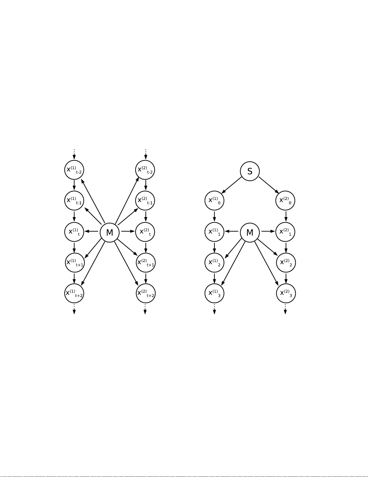
Causal inference using the algorithmic Mark o v condition Dominik Janzing and Bernhard Sc h¨ olk opf ∗ Max Planck Institute for Biolo gical Cyb ernetics, Spema nnstr. 38, 72076 T¨ ubingen, German y April 23, 2008 Abstract Inferring the causal structure that links n observ ables is usually ba sed up on detecting sta tistica l depe ndence s and choosing simple graphs that make the joint mea sure Marko via n. Here we arg ue why c a usal inference is also p ossible when only single obser v ations ar e pr esent. W e develop a theory how to generate causa l gra phs explaining s imila rities b etw een single o b- jects. T o this end, we r eplace the notio n of co nditional stochastic indep endence in the causal Marko v co ndition with the v anishing of conditional algorithmic mutual infor mation and descr ib e the corres po nding causa l inference r ules. W e ex plain w hy a c o nsistent reformulation o f causal inference in terms of a lgorithmic complex- it y implies a new inference principle that takes into account a lso the complexity of conditional probability densities, making it p oss ible to select among Marko v equiv alent ca usal graphs. This insight provides a theore tica l foundation o f a heuristic principle pr op osed in earlie r work. W e a lso discuss how to replace K olmogor ov complexit y with de cidabl e complexity criteria . This can b e seen as an algo rithmic ana log of replacing the empir ic a lly undecidable ques tion of statistical independenc e with practical indep endence tests that are bas e d o n implicit or explicit assumptions on the underlying distribution. ∗ email: { dominik. janzing,bernhard.s cho elkopf } @tuebingen.mpg.de 1 Con ten ts 1 In tro duction to causal inference from statistical data 2 1.1 Causal Markov condition . . . . . . . . . . . . . . . . . . . . . . . . . . . . . . . . . 2 1.2 Seeking for new statistical inference r ules . . . . . . . . . . . . . . . . . . . . . . . . 6 2 Inferring causal relatio ns among individual ob jects 8 2.1 Algorithmic mutual informatio n . . . . . . . . . . . . . . . . . . . . . . . . . . . . . . 9 2.2 Marko v condition for algor ithmic dep endences among individua l ob jects . . . . . . . 13 2.3 Relative causality . . . . . . . . . . . . . . . . . . . . . . . . . . . . . . . . . . . . . . 19 3 No vel statistical inference rules from the algori thmic Mark ov conditi o n 20 3.1 Algorithmic indep endence o f Markov kernels . . . . . . . . . . . . . . . . . . . . . . . 2 0 3.2 Resolving statistical ensembles into individual o bserv ations . . . . . . . . . . . . . . 26 3.3 Conditional density estimatio n on subsa mples . . . . . . . . . . . . . . . . . . . . . . 30 3.4 Plausible Markov kernels in time ser ies . . . . . . . . . . . . . . . . . . . . . . . . . . 34 4 Decidable mo diﬁcations of the inference rule 36 4.1 Causal inference using symmetr y co nstraints . . . . . . . . . . . . . . . . . . . . . . 3 6 4.2 Resource-b o unded complexity . . . . . . . . . . . . . . . . . . . . . . . . . . . . . . . 42 5 Conclusions 44 1 In tro d u ction to causal inference from statistical data Causal inference from statistical data has attra c ted increa sing in terest in the past decade. In contrast to traditional s tatistics where statistical dep endences are only taken to prove that some kind o f r e la tion b e t ween r andom v aria bles exis ts , ca usal inference metho ds in ma chine learning are explicitly designed to generate hypotheses on ca usal dir ections a utomatically based up on statistical independenc e tests [1, 2]. The cr ucial ass umption connecting statistics with ca us ality is the ca us al Marko v co ndition explained b elow after we have introduced some notatio ns a nd terminology . W e denote rando m v ariables by capita ls and their v alues by the corres p o nding lowercase letters. Let X 1 , . . . , X n be random v a r iables and G b e a directed acy clic graph (D AG) representing the causal structure where an a rrow from no de X i to no de X j indicates a direct c ausal eﬀect. Here the term dir e ct is understo o d with resp ect to the chosen set of v ariables in the sens e that the information ﬂow betw e e n the tw o v ariables cons ide r ed is not pe rformed v ia using o ne or mor e of the other v ar iables as intermediate no des. W e will next brieﬂy rephra se the p ostulates that are required in the statistical theor y of inferr ed ca usation [2, 1]. 1.1 Causal Mark ov condition When we consider the causal structure that links n r andom v aria bles V := { X 1 , . . . , X n } we will implicitly a s sume that V is causa lly s uﬃcient in the sense that all common ca uses o f tw o v ariable s in V are also in V . Then a causal hypothesis G is only acceptable a s po tential causal structure if the joint distribution P of X 1 , . . . , X n satisﬁes the Markov condition with r esp ect to G . There are several fo rmulations of the Markov condition that a r e known to c oincide under some technical condition (see Lemma 1). W e will ﬁrst in tr o duce the following version which is so metimes r eferred to a s the p ar ental o r the lo c al Markov condition [3]. 2 T o this end, we introduce the following notations. P A j is the set of par ents of X j and N D j the set of non-descendants o f X j except its e lf. If S, T , R a r e sets of rando m v aria bles, S ⊥ ⊥ T | R mea ns S is statistically indep endent of T , given R . P ostulate 1 (statisti cal causal Mark o v conditi on, l o cal) If a dir e cte d acyclic gr aph G formalizes the c ausal struct ur e among the r andom variables X 1 , . . . , X n . Then X j ⊥ ⊥ N D j | P A j , for al l j = 1 , . . . , n . W e ca ll this p os tulate the statistic al ca usal Markov condition b ecause we will later introduce a n algorithmic v ers io n. The fact that conditional ir relev ance not only o ccur s in the context of st atistic al depe ndence s has b een emphasized in the literatur e (e.g. [4, 1]) in the context o f describing abstra ct prop erties (like semi-gra phoid axio ms) o f the relation · ⊥ ⊥ · |· . W e will therefor e s tate the ca usal Marko v co ndition also in a n a bstract form that do es not r efer to any sp eciﬁc notion of conditional informational irrelev ance: P ostulate 2 (abstract causal Mark o v condition, lo cal) Given al l the dir e ct c auses of an observable O , it s n on-eﬀe cts pr ovide no additional information on O . Here, observ ables denote something in the real world that can be observed a nd the observ ation of which ca n b e forma lized in terms of a mathematica l la nguage. In this paper , observ ables will either b e random v aria bles (formalizing statistical quan tities) or they will b e strings (forma liz- ing the description o f ob jects). Accor dingly , infor mation will be statistic al o r algorithmic mutual information, resp ectively . The imp or tance of the ca usal Markov condition lies in the fact that it links causal terms like “direct causes” and “ non-eﬀects” to informational relev ance of o bs erv ables. The lo cal Marko v condition is ra ther intuit ive be c ause it echoes the fact that the infor mation ﬂows from direc t ca uses to their eﬀect and every depe ndence b etw ee n a no de and its non-descendants inv olves the direct causes. How ever, the indep endences postula ted b y the lo ca l Marko v condition imply a dditio nal independenc e s . It is there fore har d to decide whether an indep endence must hold for a Mar ko vian distribution or not, solely on the basis of the lo c al formulation. In co nt r ast, the globa l Marko v condition makes the complete set of indep endences o bvious. T o sta te it we ﬁrst hav e to in tr o duce the following g raph-theor etical conc e pt. Deﬁnition 1 (d-separation) A p ath p in a DAG is said to b e d-sep ar ate d (or blo cke d) by a set of no des Z if and only if 1. p c ontains a chain i → m → j or fork i ← m → j such that t he m idd le no de m is in Z , or 2. p c ontains an inverte d fork (or c ol lider) i → m ← j such t hat the midd le no de m is not in Z and su ch t hat no desc endant of m is in Z . A set Z is said to d-sep ar ate X fr om Y if and only if Z blo cks every (p ossibly undir e cte d) p ath fr om a n o de in X to a no de in Y . The following Lemma shows that d- separatio n is the cor rect conditio n for deciding whether an independenc e is implied by the lo cal Markov co nditio n [4], Theor em 3 .27. Lemma 1 (equiv alen t Mark o v condition s ) L et P ( X 1 , . . . , X n ) have a density P ( x 1 , . . . , x n ) with r esp e ct to a pr o duct me asu re. Then the fol lowing thr e e statement s ar e e quivalent: 3 I. Re cursiv e form: P admits the factoriza t ion P ( x 1 , . . . , x n ) = n Y j =1 P ( x j | pa j ) , (1) wher e P ( . | pa j ) is shorthand for the c onditiona l pr ob ability density, given the values of al l p ar ents of X j . II. Lo cal (or paren tal) Mark o v conditio n: for every no de X j we have X j ⊥ ⊥ N D j | P A j , i.e., it is c onditional ly indep endent of its non-desc endants (exc ept itself ), given its p ar ents. II I. Global Mark o v conditi on: S ⊥ ⊥ T | R for al l thr e e sets S , T , R of no des for which S and T ar e d-sep ar ate d by R . Mor e over, the lo c al and the glob al Markov c ondition ar e e quivalent even if P do es not have a density with r esp e ct to a pr o duct me asur e. The co nditional densities P ( x j | pa j ) ar e also called the Markov kernels relative to the hypothet- ical causal graph G . It is imp orta nt to note that every choice o f Ma rko v kernels deﬁne a Ma rko via n density P , i.e., the Ma rko v kernels deﬁne exactly the s et of fr e e para meters remaining after the causal s tructure has b een sp eciﬁed. T o select gr aphs among all those that r ender P Markovian, we also need an a dditional po stulate: P ostulate 3 (causal faithfulness ) Among al l gr aphs G for which P is Markovian, pr efer t he ones for which al l the observe d c onditional indep endenc es in t he joint me asur e P ( X 1 , . . . , X n ) ar e imp ose d by the Markov c onditio n . The idea is that the set of obser ved independences is t ypical for the caus al structure under consideratio n rather than be ing the result o f sp eciﬁc choices o f the Markov kernels. This b ecomes even more in tuitive when we res trict o ur atten tio n to rando m v ariables with ﬁnite v alue set and observe that the v alues P ( x j | pa j ) then deﬁne a natural parameteriza tio n of the set of Markovian distributions in a ﬁnite dimensiona l s pace. The non-faithful distributions form a submanifold of low er dimension, i.e., a set of Leb esgue mea s ure zero [5]. They therefore a lmost surely don’t o ccur if w e a ssume that “ nature cho oses” the Ma rko v kernels for the diﬀerent no des indep endently according to some density on the para meter spac e . The ab ov e “zer o Leb esg ue mea sure a rgument” is close to the s pirit o f Bayesian approaches [6], where priors o n the set of Mar ko v kernels are sp eciﬁed for every p o ssible hypothetica l causal DA G and causal infer ence is p er formed by maximizing pos terior probabilities for h yp othetical D AGs, given the obse rved data. This pro ce dur e leads to a n implicit preference o f faithful structures in the inﬁnite sa mpling limit given some natura l conditions for the pr io rs on the parameter space . The assumption tha t “ nature choo s es Markov kernels indep endently”, which is also part o f the Bay esia n approach, will turn o ut to b e c losely related to the alg o rithmic Markov condition p o stulated in this pap er. W e now discuss the justiﬁcation of the statistical causal Mar ko v condition b ecause we w ill la ter justify the algorithmic Markov condition in a similar way . T o this end, we introduce functional mo dels [1]: 4 P ostulate 4 (functional mo de l of causalit y) If a dir e cte d acyclic gr aph G formalizes the c ausal r elation b etwe en the r andom variables X 1 , . . . , X N then every X j c an b e written as a deterministic fu n ction of P A j and a noise variable N j , X j = f j ( P A j , N j ) , wher e al l N j ar e jointly indep endent. Then we hav e [1 ], Theorem 1.4.1: Lemma 2 (Mark o v condition in functional mo dels) Every joint distribution P ( X 1 , . . . , X n ) gener ate d ac c or ding to the fu n ctional mo del in Postulate 4 satisﬁes the lo c al and the glob al Markov c ondition r elative to G . W e rephra se the pro of in [1] b eca use our pro o f for the algorithmic version will re ly o n the sa me idea. Pro of of Lemma 2: extend G to a gra ph ˜ G with no des X 1 , . . . , X n , N 1 , . . . , N n that additionally contains an arrow from each N j to X j . The given joint distributio n of nois e v ar iables induces a joint distribution ˜ P ( X 1 , . . . , X n , N 1 , . . . , N n ) , that satisﬁes the lo cal Markov condition with r esp ect to ˜ G : ﬁrs t, every X j is completely determined by its parents mak ing the condition trivial. Second, every N j is parentless and thus w e have to chec k that it is (unconditiona lly ) indep e nden t of its non- descendants. The latter ar e deterministic functions of { N 1 , . . . , N n } \ { N j } . Hence the indep endence follows fro m the joint indep endence of all N i . By Lemma 1, ˜ P is also glo bally Markovian w.r .t. ˜ G . Then we obse r ve that N D j and X j are d-separa ted in ˜ G (where the par ent s and non-desce ndants ar e deﬁned with res p ec t to G ). Hence P satisﬁes the lo cal Markov condition w.r.t. G and hence als o the global Ma rko v condition.  F unctional mo dels formalize the idea that the outcome of an exper iment is completely deter - mined by the v alues o f all relev ant para meters where the only uncertaint y stems from the fact that some of these par ameters are hidden. Even tho ugh this kind of determinism is in contrast with the commonly a ccepted interpretation of q uantum mechanics [7], we still consider functional mo dels a s a helpful fra mework for dis c ussing causality in real life since q uantum mechanical laws refer mainly to pheno mena in micro-physics. Causal inference using the Markov condition and the faithfulness assumption has b een imple- men ted as causal lear ning algorithms [2]. The following fundamental limitations of these metho ds deserve our further attention: 1. Markov e qu ivalenc e: There are only few cases where the inference rules provide unique c a usal graphs. Often o ne ends up with a larg e cla ss of Markov equiv alent graphs, i.e., g raphs that ent a il the same set o f indep endences. F or this r e a son, additional inference rules are desirable. 2. Dep endenc e on i.i.d. sampli n g: the whole setting of causal inference r elies on the a bility to sample rep eatedly and indep endently from the same joint distr ibutio n P ( X 1 , . . . , X n ). As op- po sed to this assumption, ca us al inference in real life als o deals with pro bability distributions that c ha nge in time a nd often o ne infers causal relations among single observ ations without referring to statistics at all. The idea of this pap er is to develop a theory of probability-free ca usal inference that helps to construct causa l hypotheses based on similarities of single o b jects. Her e, similarities will b e deﬁned 5 by compar ing the length o f the sho rtest descr iption o f single o b jects to the length of their s hortest joint description. Despite the analogy to ca usal infere nce from statistical da ta (which is due to known ana logies b etw een statistica l and a lgorithmic informa tion theory) our theory also implies new st atistic al inference rules. In other words, our approach to addr ess weakness 2 a lso yields new metho ds to address 1. The pap er is structured as follows. In the remaining part of this Section, i.e., Subsection 1.2, we describ e recent appr oaches from the litera ture to caus al inferenc e from statistica l da ta that addres s problem 1 ab ov e. In Sec tion 2 we develop the general theory on inferring ca usal relations among individual ob jects ba s ed on algo rithmic information. This fra mework app ears , at ﬁrst s ight, as a straightforward adaption of the statistica l framework (using well-known corr esp ondences b etw een statistical and algor ithmic infor mation theory). How ever, Section 3 describ es that this implies novel causal inference rules for statistic al inference becaus e non-stat ist ic al algorithmic dep endences can even o ccur in da ta that were obtained from s tatistical sampling. In Section 4 we describ e how to replace causa l inference rules ba s ed on the uncomputable algorithmic information with decida ble criteria that are still motiv ated by the uncomputable idealiza tion. The table in ﬁg. 1 summarizes the analogie s b etw ee n the theory of statistica l a nd the theo ry of algorithmic causal infer ence de s crib ed in this pa pe r . The diﬀerence s , howev er, which a re the main sub ject of Sections 3 to 4, can har dly b e repres ented in the table. 1.2 Seeking for new statistical inference rules In [8] and [9] we hav e prop osed causa l inference rules that are bas ed on the idea that the factoriza tion of P (caus e , eﬀect) into P (eﬀect | cause) and P (cause) typically leads to simpler terms than the “artiﬁcial” factor ization in to P (eﬀect) P (cause | eﬀect). The gener alization o f this pr inciple rea ds : Among all graphs G that r ender P Marko vian pre fer the one for which the decomp osition in eq. (1) yields the simplest Marko v kernels. W e hav e calle d this v ague idea the “pr inc iple of plausible Marko v kernels”. Before we desc rib e several optio ns to deﬁne simplicit y we describ e a simple exa mple to illustrate the idea. Assume we have observed that a binary v a riable X (with v alues x = − 1 , 1) and a contin uous v aria ble Y (with v alues in R ) ar e distributed according to a mixtur e of tw o Gaussia ns (see ﬁg. 2 ). Since this will simplify the further discussion let us as s ume that the tw o comp onents are equally w e ig hted, i.e., P ( x, y ) = 1 2 1 σ √ 2 π e − ( y − µ − xλ ) 2 2 σ 2 , where λ determines the shift of the mean ca used by switching b etw ee n x = 1 and x = − 1 . The margina l P ( Y ) is given by P ( y ) = 1 2 1 σ √ 2 π  e − ( y − µ + λ ) 2 2 σ 2 + e − ( y − µ − λ ) 2 2 σ 2  . (2) One will pre fer the causal structure X → Y compare d to Y → X b ecause the former ex plains in a natural wa y why P ( Y ) is bimo dal: the eﬀect of X on Y is simply to s hift the Ga us sian distribution by 2 λ . In the latter mo del the bimo dality of P ( Y ) remains unexplained. T o prefer one causal mo del to another o ne b e c ause the co rresp onding conditio na ls are simpler se e ms to b e a natural a pplication of Oc c a m’s Ra zor. How ever, Section 3 will show that such an inference rule als o follows from the theory developed in the presen t pap er when simplicity is meant in the sense of low Ko lmogorov complexity . In the remaining pa r t o f this section we will sketc h so me a pproaches to implement the “principle of plausible Markov kernels” in pra ctical applications. In [8] we have deﬁned a family o f “plaus ible Marko v kernels” by conditiona ls P ( X j | P A j ) that are seco nd orde r exp onential mo dels , i.e., log P ( x j | pa j ) is a p olyno mial of order t wo in the v ariables 6 statistical algorithmic observ ables random v ariables sequences of strings (v ertices of a D A G) observ ations i.i.d. sampled data strings conditional indep endence X ⊥ ⊥ Y | Z x ⊥ ⊥ y | z .. m .. m I ( X ; Y | Z ) = 0 I ( x : y | z ) + = 0 I. recursion form u la P ( x 1 , . . . , x n ) K ( x 1 , . . . , x n ) = = Q j p ( x j | pa j ) P j K ( x j | pa ∗ j ) I I. lo cal Mark ov condition X j ⊥ ⊥ N D j | P A j x j ⊥ ⊥ nd j | pa ∗ j I I I . global Mark ov d-separation d-separation condition ⇒ ⇒ statistica l indep endence algorithmic indep endence equiv alence of I -I I I Theorem 3.27 Theorem 3 in [4] functional mo dels Section 1.4 P ostulate 6 in [1] functional mo dels Theorem 1.4.1 Theorem 4 imply Mark o v condition in [1] decidable dep en d ence assumptions on Section 4 criteria joint distrib ution Figure 1: Analogie s b etw een statistica l a nd algor ithmic causal inference 7 Figure 2: Observed joint distributio n o f X and Y consisting o f tw o Gaussians of equal width shifted a gainst each other . { X j } ∪ { P A j } up to so me a dditive partition function (for normalizatio n) that dep ends only on the v ariables P A j . F or every hypo thetical causal graph, one thus o btains a family of “plausible joint distributions P ( X 1 , . . . , X n )” tha t are pro ducts of the plausible Markov kernels. Then we pr efer the ca usal dir e ction for whic h the plaus ible joint distributions pr ovide the b est ﬁt for the giv en observ ations. In [9] we have pro po sed the following principle for causal inference: Given a joint distribution of the r andom v ariables X 1 , . . . , X n , prefer a causal structure for which n X j =1 C ( P ( X j | P A j )) (3) is minimal, where C is some complexity meas ure on conditional probability dens ities. There is also another rece nt prop osa l for new inference rule s that refer s to a rela ted simplicity assumption, thoug h for mally quite diﬀerent from the o nes ab ove. The a uthors o f [10] observe that there are joint distributions of X 1 , . . . , X n that can b e explained by a linea r mo del with a dditive non-Gaussian noise for one causal directio n but req uire non-linear causa l inﬂuence for the other causal dir e c tions. F or real da ta they prefer the causal g raph for which the obs e rv ations are clo ser to the linear mo del. T o justify the belief that c o nditionals that corresp ond to the true causal direc tion tend to b e simpler than non-causal conditiona ls (which is co mmo n to a ll the approaches ab ove) is one of the main g oals of this pap er. 2 Inferring causal relations among individual ob jects It ha s b een emphasized [1 ] that the application o f c ausal inference principles often be neﬁts fro m the non-determinism of ca usal r e lations b etw een the observed random v ariables. In co nt r ast, h uman learning in r e a l-life often is ab o ut quite deterministic relations. Apart from that, the most impor tant diﬀerence b etw een human causal lea rning and the inference r ules in [2 , 1] is that the former is also ab out causal relations among single ob jects and do es not necessar ily requir e s ampling. Assume, for instance, that the co mpa rison of tw o texts s how similarities (see e.g. [11]) such that the author of the text that app ear ed la ter is blamed to hav e copied it from the other one o r bo th are blamed to hav e co pied from a third one. The statement that the texts are similar could b e based o n a statistical analys is of the o ccurrences of certain words o r letter sequences. How ever, s uch kind of 8 simple statistical tests c an fail in b oth dir ections: In Subsection 2.2 (b efore Theor em 3) we will discuss an example s howing that they ca n erroneo us ly infer ca usal relations even thoug h they do not ex ist. This is b ecause pa rts that ar e common t wo b oth ob jects, e.g., the t wo texts, are only suitable to prov e a causal link if they are not “to o straig htf o rward” to co me up with. On the other hand, ca usal rela tions can gener ate similarities b etw een texts for whic h e very eﬃcient statistical analysis is b elieved to fa il. W e will describe an idea from cryptogr aphy to show this. A crypto system is ca lled ROR-CCA-secure (Real or Random under Chosen Ciphertext A ttacks) if there is no eﬃcient metho d to decide whether a text is random or the encr ypted version of some known text without knowing the key [12 ]. Giv en that there a re ROR-CCA-secure schemes (whic h is unknown but b elieved by crypto grapher s ) we hav e a causa l relation leading to s imila rities that are not detected by any kind of simple counting sta tis tics . How ever, o nce a n attack er has found the key (ma y b e by exhaustive s earch), he recog niz e s similar ities b etw een the encr ypted text and the plain text and infers a c a usal relation. This alrea dy sugges ts tw o things: (1) detecting similarities inv olves se ar ching ov er po tential rules how pro p e rties of o ne ob ject can b e alg orithmically derived from the structure of the o ther . (2) It is likely that inferr ing causal relatio ns ther efore relies on c omputational ly infe asible decisions (if computable at all) on whether tw o ob jects hav e informa tion in common or not. 2.1 Algorithmic mutual information W e will now describ e how the informatio n one ob ject provides a b o ut the other ca n b e measured in terms of K olmogor ov complexity . W e start with some notation and terminology . Below, strings will alwa ys b e bina ry string s since every description given in terms of a diﬀer ent a lphab et can be co nverted into a binar y w ord. The set of binary strings of a rbitrar y length will be denoted by { 0 , 1 } ∗ . Recall that the Kolmo gorov complexity K ( s ) of a string s ∈ { 0 , 1 } ∗ is deﬁned as the length of the shortest pro g ram that gener ates s using a previously deﬁned universal T uring machine [13, 14, 15, 16, 17, 1 8, 19]. The conditional Ko lmogorov complexity K ( t | s ) [18] of a string t given another s tring s is the le ng th o f the shortest prog ram that ca n gener a te t from s . In or der to keep our notation simple we use K ( x, y ) to refer to the co mplex it y of the conca tenation of x, y . W e will mos tly have e q uations that are v a lid o nly up to additive constant terms in the sense that the diﬀerence b etw een b oth s ides do es not dep end o n the strings inv o lved in the eq ua tion (but it may dep end on the T uring ma chines they r efer to). T o indicate such constants w e denote the corres p o nding equa lity by + = and lik ewis e for inequalities. In this context it is impo r tant to note that the n umber n o f no des of the causa l gra ph is consider e d to b e a cons ta nt . Mor eov er, for every string s we deﬁne s ∗ as its shor test description. If the la tter is not unique, we consider the ﬁrst one in an le xicogra phic or der. It is necessary to distinguish b etw een K ( ·| s ) a nd K ( ·| s ∗ ). This is bec ause there is a trivial alg orithmic metho d to g enerate s from s ∗ (just apply the T uring machine to s ∗ ), but there is no algo r ithm of length O (1) that computes the shor test description s ∗ from a general input s . One can show [1 9] that s ∗ ≡ ( s, K ( s )). Here, the equiv alence symbol ≡ means that b oth sides can b e obtained from ea ch other by O (1) pr ogra ms . The following equatio n for the joint algor ithmic information of tw o strings x, y will b e useful [20]: K ( x, y ) + = K ( x ) + K ( y | x ∗ ) = K ( x ) + K ( y | x, K ( x )) . (4) The conditional version rea ds [2 0]: K ( x, y | z ) + = K ( x | z ) + K ( y | x, K ( x | z ) , z ) (5) The most imp ortant notion in this pap er will b e the algor ithmic mutual info rmation measuring the amount of algor ithmic information that tw o ob jects have in common. F ollowing [21] we deﬁne: 9 Deﬁnition 2 (algorithmic m utual information) L et x, y b e two s t rings. Then the algorithmic mutual information of x, y is I ( x : y ) := K ( y ) − K ( y | x ∗ ) . The mutual information is the n umber of bits that can b e sav ed in the descr iption of y when the sho rtest description o f x is alr eady known. The fact that one us e s x ∗ instead of x ens ures that it coincides with the symmetric expres s ion [21]: Lemma 3 (symmetric version of algorithmic mutual information) F or two strings x, y we have I ( x : y ) + = K ( x ) + K ( y ) − K ( x, y ) . In the following sections, non-v anishing m utual information will b e ta ken as a n indicator for causal relations, but mor e deta ile d information on the causa l str uc tur e will be inferred fro m c on- ditional m utual informatio n. This is in contrast to appr oaches from the liter ature to measure similarity versus diﬀer ences of single ob jects that w e br ieﬂy review now. T o meas ure diﬀerences betw e e n sing le ob jects, e.g. pictures [22, 2 3], one deﬁnes the information distanc e E ( x, y ) b etw een the tw o co rresp onding str ings as the length of the shortest progr a m that computes x from y and y from x . It can b e shown [22] that E ( x, y ) log = max { K ( x | y ) , K ( y | x ) } , where log = means e quality up to a lo g arithmic term. How ever, whether E ( x, y ) is s mall or larg e is not an appropriate condition for the exis tence and the strength of a causal link. Complex ob jects can ha ve muc h information in commo n even though their distance is larg e. In order to obtain a measure that rela tes the amo un t of infor mation that is disjoint for the t wo s tr ings to the amount they share, Li et al. [23] and Bennett et al. [1 1] use the “ normalized distance measure” d s ( x, y ) := K ( x | y ∗ ) − K ( y | x ∗ ) K ( x, y ) + = 1 − I ( x : y ) K ( x, y ) , or d ( x, y ) = max { K ( x | y ) , K ( y | x ) } max { K ( x ) , K ( y ) } . The intuitiv e meaning of d s ( x, y ) is o bvious fr o m its dire c t r e lation to mut ua l infor mation, and 1 − d ( x, y ) measures the fraction of the infor mation of the more complex str ing that is sha red with the other one. Bennett et al. [11] pr op ose to c o nstruct evolutionary histor ies of chain letters using such kinds o f information distance measures . How ever, like in statistica l causal inference, inferring adjacencies on the basis of strongest dep endences is only p os sible for simple causal structur es like trees. In the g eneral case, non-a djacent no des can share more information than adjac e nt ones when information is propaga ted via more tha n one path. Instead of constructing causal neighborho o d relations by compa ring information distances we will therefor e use conditional mutual infor mation. In order to deﬁne its algor ithmic version, we ﬁr st obser ve that Deﬁnition 2 can b e rewritten int o the les s c o ncise form I ( x : y ) + = K ( y ) − K ( y | x, K ( x )) . This fo r mula generaliz e s more natura lly to the co nditional analog [20]: Deﬁnition 3 (conditional alg orithmic mutual informatio n information) L et x, y , z b e thr e e s t rings. Then the c onditional m utual algorithmic information of x, y , given z is I ( x : y | z ) := K ( y | z ) − K ( y | x, K ( x | z ) , z ) . 10 As shown in [2 0] (Remark I I.3), the conditional m utua l infor mation a lso is symmetric up to a constant term: Lemma 4 (symmetric alg o rithmic conditi onal mutual information) F or thr e e st rings x, y , z one has: I ( x : y | z ) + = K ( x | z ) + K ( y | z ) − K ( x, y | z ) . Deﬁnition 4 (algorithmic conditional indep endence) Given t hr e e strings x, y , z , we c al l x c onditional ly indep endent of y , given z (denote d by x ⊥ ⊥ y | z ) if I ( x : y | z ) ≈ 0 . In wor ds: Given z , t he additional know le dge of y do es not al low us a str onger c ompr ession of x . This r emains t r u e if we ar e given the Kolmo gor ov c omplexity of y , given z . The theory dev elo p ed b e low will describ e la ws where symbols lik e x, y , z represe nt ar bitrary strings. Then one can alwa y s think of se quenc es of string s of incr easing complex it y a nd sta tement s like “the equation holds up to constant terms” are well-deﬁned. W e will then understa nd conditional independenc e in the sense of I ( x : y | z ) + = 0 . How ever, if we a re talking a b out three ﬁxed string s that represent ob jects in r e al-life , this do es not make sense and the threshold for considering tw o strings dep endent will heavily depend on the c o ntext. F or this rea son, we will not sp ecify the symbol ≈ any fur ther . This is the same arbitr ariness as the cutoﬀ rate for statistical dep endence tests. The deﬁnitions and lemma s presented so far were stro ngly motiv ated by the statistical analo g. Now we wan t to fo cus on a theorem in [21] that pr ovides a mathematical relationship b etw een algorithmic a nd statis tica l mutual information. First we rephr ase the following theorem Theorem 7.3.1 of [18], showing that the Ko lmogor ov complexity of a random string is approximatively given by the e nt r opy of the underlying probability distributio n: Theorem 1 (en tropy and Kolmogorov compl exit y) L et x = x 1 , x 2 , · · · , x n b e a string whose symb ols x j ∈ A ar e dr awn i.i.d . fr om a pr ob abili t y distri- bution P ( X ) over the ﬁnite alphab et A . Slightly overlo ading notation, set P ( x ) := P ( x 1 ) · · · P ( x n ) . L et H ( . ) denote t he Shannon entr opy of a pr ob ability distribution. Then ther e is a c onstant c such that H ( P ( X )) ≤ 1 n E ( K ( x | n )) ≤ H ( P ( X )) + |A| log n n + c n ∀ n , wher e E ( . ) is short hand for t he ex p e cte d value with r esp e ct to P ( x ) . Henc e lim n →∞ 1 n E ( K ( X )) = H ( P ( X )) . How ever, for our purp ose, w e need to see the relation b etw een algor ithmic and statistical mutual information . If x = x 1 , x 2 , · · · , x n and y = y 1 , y 2 , · · · , y n such tha t each pair ( x j , y j ) is drawn i.i.d. from a jo in t distribution P ( X , Y ), the theorem already shows that lim n →∞ 1 n E ( I ( x : y )) = I ( X ; Y ) . This ca n b e seen by writing statis tica l mutual infor mation as H ( P ( X )) + H ( P ( Y )) − H ( P ( X, Y )) . 11 The ab ov e tr anslations betw ee n entrop y and algo rithmic information refer to a particular setting and to sp ecial limits. The fo cus o f this pap er is ma inly the situatio n where the a b ove limits a r e not justiﬁed. Befor e we rephras e Theore m 5.3 in [2 1] whic h provides insig h ts into the general case, we recall tha t a function f is called r ecursive if there is a progr am on a T uring machine that co mputes f ( x ) fro m the input x , and ha lts on all po ssible inputs. Theorem 2 (statistical and algorithm ic m utual information) Given string-value d r andom variables X , Y with a r e cursive pr ob ability mass function P ( x, y ) over p airs ( x, y ) of strings. We then have I ( X ; Y ) − K ( P ) + ≤ E ( I ( x : y )) + ≤ I ( X ; Y ) + 2 K ( P ) , wher e K ( P ) is the length of the shortest pr eﬁx-fr e e pr o gr am that c omputes P ( x, y ) fr om ( x, y ) . W e wan t to provide an intuition a bo ut v ar io us asp ects of this theo rem. (1) If I ( X ; Y ) is la r ge co mpared to K ( P ) the exp ected alg orithmic mutual information is do minated by the s tatistical mut ua l information. (2) If K ( P ) is no lo nger assumed to b e small, s tatistical dep endences do not necessa rily ensure that the knowledge of x allows us to compres s y further than without knowing x . It could b e that the description o f the statistica l dep endences requir es mor e memory s pa ce than its knowledge would sav e. (3) On the other hand, k nowledge o f x could allow us to co mpress y even in the case of a pro duct measure o n x and y . Consider , for instance, the case that we have the p oint mass dis tribution on the pair ( x, y ) w ith x = y . T o describ e a mo re sophisticated exa mple g eneralizing this case we ﬁrst hav e to introduce a family o f pro duct pr o bability distr ibutions on { 0 , 1 } n that we will need s everal times throughout the pap er. Deﬁnition 5 (Deﬁning pro duct di stributions by strings ) L et P 0 , P 1 b e two pr ob ability distributions on { 0 , 1 } and c b e a binary string of length n . Then P c := P c 1 ⊗ P c 2 ⊗ · · · ⊗ P c n deﬁnes a distribution on { 0 , 1 } n . We wil l later also ne e d the fol lowing gener alization: If P 00 , P 01 , P 10 , P 11 ar e four distributions on { 0 , 1 } , then P c,d := P c 1 ,d 1 ⊗ P c 2 ,d 2 ⊗ · · · ⊗ P c n ,d n deﬁnes also a family of pr o duct me asur es on { 0 , 1 } n that is lab ele d by two strings. Denote by P ⊗ m c the m - fold copy of P c from Deﬁnition 5. It describ es a distributio n o n { 0 , 1 } nm assigning the probbaility P ⊗ m c ( x ) to x ∈ { 0 , 1 } nm . If Q ( x, y ) := P ⊗ m c ( x ) P ⊗ m c ( y ) , knowledge o f x in the typical cas e provides knowledge of c , provided m is large enough. Then we can compress y b etter than without knowing x b ecause we do not hav e to describ e c a ny more. Hence the algorithmic mutual information is la rge a nd the statistica l mutual information is zer o bec ause Q is by construction a pro duct dis tribution. In other words, a lgorithmic dep endences in a setting with i.i.d sampling ca n ar ise from statistical dep endences a nd from algo r ithmic dep e ndenc e s betw e e n pro bability distributions. 12 2.2 Mark o v condition for algorithmic dep endences among individual ob- jects Now we state the caus al Mar ko v co ndition fo r individual ob jects a s a p o stulate that links alg orithmic m utual dependences with causal s tructure: P ostulate 5 (algori thmic causal Mark o v condition) L et x 1 , . . . , x n b e n strings r epr esenting descriptio n s of observations whose c ausal c onne ctions ar e formalize d by a dir e cte d acyclic gr aph G with x 1 , . . . , x n as no des. L et pa j b e the c onc atenation of al l p ar ents of x j and nd j the c onc atenation of al l its n on-desc endants exc ept x j itself. Then x j ⊥ ⊥ nd j | pa ∗ j . As in Deﬁnition 4 , the appr opria t e cut-oﬀ ra t e for r eje cting G when I ( x j : n d j | pa ∗ j ) > 0 wil l n ot b e sp e ciﬁe d her e. This for mulation is a natural interpretation of Postulate 2 in ter ms of algor ithmic indep endences. The only p oint that remains to b e justiﬁed is why we condition on pa ∗ j instead of pa j , i.e., why we are given the optimal joint compr ession of the par ent strings. The ma in rea son is that this turns out to yield nice statements on the equiv alence of diﬀerent Mar ko v conditions (in analo gy to Lemma 1 ). Since the diﬀerences b etw een I ( x j : nd j | pa j ) and I ( x j : nd j | pa ∗ j ) can only be log arithmic in the string lengths 1 we will not fo cus on this is sue a ny further. If we apply Postulate 5 to a trivial gr a ph co ns isting o f tw o unconnected no des, we obtain the following s ta tement . Lemma 5 (causal principl e for algorithm i c information) If the m u tual information I ( x : y ) b etwe en two obje cts x, y is signiﬁc antly gr e ater than zer o they have s ome kind of c ommon p ast. Here, commo n past betw ee n t wo ob jects means that o ne ha s c ausally inﬂuenced the other or there is a thir d one inﬂuencing b o th. The s tatistical version of this principle is part of Reic henbach’s principle of the common cause [24] s ta ting that statistical depe ndenc e s b etw een random v aria bles 2 X and Y a re alwa ys due at least one of the following thr ee types of causal links: (1) X is a cause of Y or (2) vic e versa or (3 ) there is a common cause Z . F or ob jects, the term “co mmon past” includes all thr ee types of ca usal relations. F or a text, for instance, it rea ds: similarities o f tw o texts x, y indicate that one author has b een inﬂuenced by the other or that b oth ha ve be e n inﬂuenced by a third one. Before w e construct a mo del of causality that mak es it p o ssible to prove the causa l Mar kov condition we wan t to discuss some ex a mples. If one discovers signiﬁcant similar ities in the genome of tw o sor ts of animals one will try to explain the similarities b y rela tedness in the sense of evolution. Usually , one would, for instance, assume such a co mmon histor y if one has identiﬁed long subs trings that both animals have in common. How ever, the following s cenario shows t wo observ ations tha t sup e rﬁcially lo ok similar, but nevertheless we cannot infer a commo n past since their algo rithmic complexity is low (implying that the alg orithmic mutual info r mation is low, to o). Assume t wo p ers ons are instructed to write down a binary string of length 1000 and b oth decide to wr ite the same str ing x = 1100 10010 0001 111110 ... . It seems stra ightforw ar d to assume tha t the per sons hav e commu nica ted and agreed up o n this choice. How ever, a fter observing that x is just the binary representation of π , one can easily imagine that it was just a coincidence that b oth wrote the same sequence. In other words, the similarities a re no lo nger signiﬁcant a fter o bserving 1 this is b ecause K ( x | y ) − K ( x | y ∗ ) = O (log | y | ), see [19 ] 2 The original form u lation considers actually dep endences b etw een events, i.e., binary v ariables. 13 that they stem from a simple rule. This shows that the length of the patter n that is co mmo n to bo th observ ations, is not a reaso na ble criter io n on whether the simila rities are signiﬁcant. T o understand the a lgorithmic ca usal Markov condition w e will study its implications as well as its justiﬁcation. In analog y to Lemma 1 we hav e Theorem 3 (equiv alence of algorithmic Mark ov conditi ons) Given the strings x 1 , . . . , x n and a dir e cte d acyclic gr aph G . Then the fol lowing c onditions ar e e quivalent: I. Re cursiv e form : the joint c omplexity is given by the sum of c omplexities of e ach no de, given the optimal c ompr ession of its p ar ents: K ( x 1 , . . . , x n ) + = n X j =1 K ( x j | pa ∗ j ) (6) II. Lo cal Mark o v condi tion: Every no de is indep endent of its non-desc endants, given t he optimal c ompr ession of its p ar ents: I ( x j : n d j | pa ∗ j ) + = 0 . II I. Global Mark o v conditi on: I ( S : T | R ∗ ) + = 0 if R d-sep ar ates S and T . Below we will therefore no long er distinguish b etw een the diﬀerent versions a nd just refer to “the algorithmic Marko v condition” . The intuit ive meaning o f eq. (6) is that the shor test des cription of all str ings is g iven b y des cribing how to g enerate every string fr o m its direct ca us es. A similar kind of “ mo dularity” of descriptions will als o occ ur later in a diﬀerent context when we consider description complexity of joint proba bilit y distributio ns . F or the pro of o f Theore m 3 we will nee d a Lemma that is an a nalogue of the obser v atio n that for any tw o random v ariables X , Y the statistical mut ua l information satisﬁes I ( f ( X ); Y ) ≤ I ( X ; Y ) for every meas urable function f . The algo r ithmic a nalog is to co nsider t wo str ings x, y and one string z that is derived fr o m x ∗ by a simple rule. Lemma 6 (monotonicity of algorithmi c information) L et x, y , z b e thr e e strings such that K ( z | x ∗ ) + = 0 . Then I ( z : y ) + ≤ I ( x : y ) . This lemma is a sp ecial case of Theo r em I I.7 in [2 0]. W e will also need the following r esult: Lemma 7 (monotonicity of conditional information) L et x, y , z b e thr e e strings. Then K ( z | x ∗ ) + ≥ K ( z | ( x, y ) ∗ ) . Note that K ( z | x ∗ ) + ≥ K ( z | x ∗ , y ) and K ( z | x ∗ ) + ≥ K ( z | x ∗ , y ∗ ) is obvious but Lemma 7 is non- trivial b ecause the star op era tion is jointly applied to x a nd y . 14 Pro of of Lemma 7: Clea rly the string x can b e deriv ed from x, y by a program of le ngth O (1). Lemma 6 ther efore implies I ( z : x ) + ≤ I ( z : x, y ) , where I ( z : x, y ) is sho r thand fo r I ( z : ( x, y )). Hence K ( z ) − K ( z | x ∗ ) + = I ( z : x ) + ≤ I ( z : x, y ) + = K ( z ) − K ( z | ( x, y ) ∗ ) . Then we obtain the statement by subtracting K ( z ) and inverting the sign.  The following lemma will only b e used in Subsectio n 3.3. W e state it here b ecause it is closely related to the ones ab ov e. Lemma 8 (generalized data pro cess i ng inequality) F or any thr e e strings x, y , z , I ( x : y | z ∗ ) + = 0 implies I ( x : y ) + ≤ I ( x : z ) . The name “data pr o cessing inequality” is justiﬁed b eca use the as sumption x ⊥ ⊥ y | z ∗ may ar ise from the t y pic a l da ta pro cessing scena r io where y is obtained from x via z . Pro of of Lemma 8: Using Lemma 7 we hav e K ( x | y ∗ ) + ≥ K ( x | ( z y ) ∗ ) (7) + = K ( x | z , y , K ( y z )) + = K ( x | z , y , K ( z ) + K ( y | z ∗ )) + ≥ K ( x | z , y , K ( z ) , K ( y | z ∗ ) + = K ( x | z ∗ , y , K ( y | z ∗ )) , where the second inequality holds b eca use K ( z ) + K ( y | z ∗ ) can obviously b e c o mputed from the pair ( K ( z ) , K ( y | z ∗ )) b y an O (1 ) progr a m. The last equality us e s , a gain, the equiv alence o f z ∗ and ( z , K ( z )). Hence we obtain: I ( x : y ) + = K ( x ) − K ( x | y ∗ ) + = K ( x | z ∗ ) + I ( x : z ) − K ( x | y ∗ ) + ≤ K ( x | z ∗ ) + I ( x : z ) − K ( x | y , K ( y | z ∗ ) , z ∗ ) + = I ( x : z ) + I ( x : y | z ∗ ) + = I ( x : z ) . The ﬁrst step is by Deﬁnition 2, the seco nd one uses Lemma 7, the third step is a direct application of ineq . (7), the fourth one is due to Deﬁnition 3, and the last s tep is b y ass umption.  Pro of o f Theorem 3: I ⇒ II I: Deﬁne a probability mass function P on ( { 0 , 1 } ∗ ) × n , i.e., the se t of n -tuples of strings, as follows. Set P ( x j | pa j ) := 1 z j 2 − K ( x j | pa ∗ j ) , (8) 15 where z j is a nor malization factor. In this context, it is imp ortant that the sy m b o l pa j refers to conditioning o n the k - tuple of string s x i that ar e parents of x j (in contrast to conditional complexities wher e we ca n in ter pret K ( . | pa ∗ j ) equally w ell as conditioning o n one string g iven by the c onc atenation of all those x i ). Note that Kra ft’s inequa lity (s e e [19], E xample 3.3.1) implies X x 2 − K ( x | y ) ≤ 1 , for every y entailing that the expres sion is indeed nor malizable by z j ≤ 1. W e hav e K ( x j | pa ∗ j ) + = − lo g 2 P ( x j | pa j ) . Then we set P ( x 1 , . . . , x n ) := n Y j =1 P ( x j | pa j ) , (9) i.e., P is by constructio n rec ur sive with resp e ct to G . It is ea sy to s e e that K ( x 1 , . . . , x n ) can be computed from P : K ( x 1 , . . . , x n ) + = n X j =1 K ( x j | pa ∗ j ) (10) + = − n X j =1 log 2 P ( x j | pa j ) = − lo g 2 P ( x 1 , . . . , x n ) . Remark ably , w e c an also compute Ko lmogorov complex ities of subsets of { x 1 , . . . , x n } from the corres p o nding marg inal pro babilities. W e start by proving K ( x 1 , . . . , x n − 1 ) + = − log 2 X x n 2 − K ( x 1 ,...,x n ) . (11) T o this end, we observe X x n 2 − K ( x 1 ,...,x n ) × = X x n 2 − K ( x 1 ,...,x n − 1 ) − K ( x n | ( x 1 ,...,x n − 1 ) ∗ ) (12) × ≤ 2 − K ( x 1 ,...,x n − 1 ) , where × = denotes equality up to a multiplicativ e co nstant. The equality follows from eq. (4) and the inequa lity is o bta ined by a pplying Kraft’s inequalit y [19] to the conditional complexity K ( . | ( x 1 , . . . , x n − 1 ) ∗ ). On the other hand we have K ( x 1 , . . . , x n − 1 ) + = K ( x 1 , . . . , x n − 1 , 0) , since adding the 1 -bit string x n = 0 certainly can b e p erfor med b y a pro gram of le ng th O (1). Hence we have X x n 2 − K ( x 1 ,...,x n ) × ≥ 2 − K ( x 1 ,...,x n − 1 , 0) × = 2 − K ( x 1 ,...,x n − 1 ) . 16 Combining this with ineq. (12) yields 2 − K ( x 1 ,...,x n − 1 ) × = X x n 2 − K ( x 1 ,...,x n ) . Using eq. (10) we obtain K ( x 1 , . . . , x n − 1 ) + = − lo g 2 X x n 2 − K ( x 1 ,...,x n ) + = − lo g 2 X x n P ( x 1 , . . . , x n ) + = − lo g 2 P ( x 1 , . . . , x n − 1 ) , which pr ov es e q uation (11). This implies K ( x 1 , . . . , x n − 1 ) + = − log 2 P ( x 1 , . . . , x n − 1 ) . Since the same arg umen t holds for marg inalizing ov er any other v ariable x j we co nclude tha t K ( x j 1 , . . . , x j k ) + = − log 2 P ( x j 1 , . . . , x j k ) , (13) for every s ubset of strings of size k with k ≤ n . This follows b y induction over n − k . Now we ca n us e the relation betw een mar ginal pr obabilities and Kolmogo rov co mplexities to show that conditiona l complexities are also g iven by the co rresp onding c onditional pro babilities, i.e., for any tw o s ubs ets S, T ⊂ { x 1 , . . . , x n } w e have K ( S | T ∗ ) + = − log 2 P ( S | T ) . Without loss of genera lity , set S := { x 1 , . . . , x j } and T := { x j +1 , . . . , x k } for j < k ≤ n . Using eqs. (4) and (13) we get K ( x 1 , . . . , x j | ( x j +1 , . . . , x k ) ∗ ) + = K ( x 1 , . . . , x k ) − K ( x j +1 , . . . , x k ) + = − log 2  P ( x 1 , . . . , x k ) /P ( x j +1 , . . . , x k )  + = − log 2 P ( x 1 , . . . , x j | x j +1 , . . . , x k ) . Let S, T , R b e three subsets of { x 1 , . . . , x n } such that R d-s e pa rates S and T . Then S ⊥ ⊥ T | R with resp ect to P beca use P s atisﬁes the recursio n (9) (see Lemma 1) 3 . Hence K ( S, T | R ∗ ) + = − log 2 P ( S, T | R ) + = − log P ( S | R ) − log 2 P ( T | R ) + = K ( S | R ∗ ) + K ( S | R ∗ ) . This pr ov es algorithmic indep endence of S and T , given R ∗ and thus I ⇒ I I I. T o show that I I I ⇒ I I it s uﬃce s to r ecall that nd j and x j are d- separated by pa j . No w we show II ⇒ I in str o ng a nalogy to the pr o of for the statistical version of this statement in [3]: Consider ﬁrst a terminal no de of G . Assume, without loss of generality , that it is x n . Hence all strings 3 Since P is, by construction, a discrete probabilit y function, P the density with resp ect to a pro duct measure is directly given by the probab ility function itself. 17 x 1 , . . . , x n − 1 are non-desce nda nt s of x n . W e thus have ( nd n , pa n ) ≡ ( x 1 , . . . , x n − 1 ) wher e ≡ means that b oth string s coincide up to a p ermutation (o n one s ide) a nd removing those strings that o ccur t wic e (on the other s ide). Due to eq. (4) we hav e K ( x 1 , . . . , x n ) + = K ( x 1 , . . . , x n − 1 ) + K ( x n | ( nd n , pa n ) ∗ ) . (14) Using, again, the equiv alence of w ∗ ≡ ( w, K ( w )) for a ny string w we have K ( x n | ( nd n , pa n ) ∗ ) + = K ( x n | nd n , pa n , K ( nd n , pa n )) + = K ( x n | nd n , pa n , K ( pa n ) + K ( nd n | pa ∗ n )) + ≥ K ( x n | nd n , pa ∗ n , K ( nd n | pa ∗ n )) + = K ( x n | pa ∗ n ) . (15) The second step follows from K ( nd n , pa n ) = K ( pa n ) + K ( nd n | pa ∗ n ). The inequality holds b eca use nd n , pa n , K ( pa n )+ K ( nd n | pa ∗ n ) can b e co mputed from nd n , pa ∗ n , K ( nd n | pa ∗ n ) via a pr ogram of length O (1). T he last step follows directly from the assumption x n ⊥ ⊥ nd n | pa ∗ n . Co m bining ine q . (1 5) with Lemma 7 yields K ( x n | ( nd n , pa n ) ∗ ) + = K ( x n | pa ∗ n ) . (16) Combining eqs. (16) and (14) we obtain K ( x 1 , . . . , x n ) + = K ( x 1 , . . . , x n − 1 ) + K ( x n | pa ∗ n ) . (17) Then statement I follows by induction over n .  T o show that the algor ithmic Mar ko v condition c an b e derived from an algo rithmic version of the functional mo del in Postulate 4 we introduce the following mo del o f causal mechanisms. P ostulate 6 (algori thmic mo del of causalit y) L et G b e a DA G formalizing the c ausal structu re among the st rings x 1 , . . . , x n . Then every x j is c ompute d by a pr o gr am q j with length O (1) fr om its p ar ents pa j and an additional input n j . We write formal ly x j = q j ( pa j , n j ) , me aning that the T u ring machine c omputes x j fr om the input pa j , n j using t he additional pr o gr am q j and halts. The inputs n j ar e jointly indep endent in the sense n j ⊥ ⊥ n 1 , . . . , n j − 1 , n j +1 , n n . By deﬁning new pr o gr ams that c ont ain n j we c an, e quivalently, dr op the assumption t hat the pr o- gr ams q j ar e simple and assume that they ar e jointly indep endent inste ad. W e could a lso hav e assumed that x j is a function f j of all its parents, but our mo del is more general since the map deﬁned b y the input-output behavior of q j need not b e a to tal function [19], i.e., the T uring machine simulating the pr o cess would not necessarily halt on al l inputs pa j , n j . The idea to represent causa l mechanisms by progr ams wr itten for some universal T ur ing machine is basica lly in the spirit of v ario us int er pretations of the Church-T uring thesis. One formulation, given by Deutsch [25], states that every pro ce s s taking plac e in the r eal world c an b e simulated by 18 a T uring ma chine. Here we assume that the wa y diﬀerent systems inﬂuence each other by physical signals can b e simulated by computation pr o cesses that exchange message s of bit strings. 4 Note that mathematics also a llows us to co ns truct strings that are linked to each other in a n unc omputable wa y . F or instance, let x b e an arbitrar y binar y string and y be deﬁned by y := K ( x ). How ever, it is har d to be lie ve that a real causal mech a nism could create such k ind of rela tions betw e e n o b jects given that one b elieves that real pr o cesses can a lwa ys b e simulated by algor ithms. These remarks are intended to give suﬃcient mo tiv ation for our mo del. Postulate 6 implies the alg orithmic ca usal Marko v co ndition: Theorem 4 (algorithmic mo del im plies Mark ov) L et x 1 , . . . , x n b e gener ate d by the mo del in Postulate 6 . Then they satisfy the algorithmic Markov c ondition with r esp e ct to G . Pro of (str aightforw a rd adaption of the pro o f of Lemma 2): E xtend G to a causal str ucture ˜ G with no des x 1 , . . . , x n , n 1 , . . . , n n . T o see that the extended set of no des satisfy the lo cal Marko v condition w.r.t. ˜ G , obs e rve ﬁrst that every no de x j is given by its pa r ents via an O (1) pr ogram. Second, every n j is parentless and (unco nditionally) indep endent of all its non-descendants b ecause they can b e computed from { n 1 , . . . .n n } \ { n j } via an O (1) pr ogra m. By Theo rem 3 the e x tended set o f no des is also glo bally Markovian w.r.t. ˜ G . The parents pa j d-separa te x j and nd j in ˜ G (here the pa r ents pa j are s till deﬁned with resp ect to G ). This implies the lo cal Markov condition for G .  It is trivia l to c onstruct examples where the causal Mar ko v condition is violated if the prog r ams q j are mutually dep endent (for instance, the trivial gra ph with tw o no des x 1 , x 2 and no edge would satisfy I ( x 1 : x 2 ) > 0 if the progr ams q 1 , q 2 computing x 1 , x 2 from an empty input are dep endent). The las t sentence of Postulate 6 makes appar ent that the me chanisms that generate caus al relations ar e ass umed to be indep endent. This is essential for the g eneral philosophy o f this pap er. T o see that such a mu tua l indep endence of mechanisms is a reasonable ass umption we recall that the ca us al gr aph is mea nt to formalize al l relev ant caus al links b etw een the ob jects. If we o bserve, for instance, that tw o no des are genera ted fro m their parents by the same complex rule we p os tulate another causal link b etw een the no des that expla ins the s imilarity o f mechanisms. 5 2.3 Relativ e causalit y This subsection expla ins why it is sensible to deﬁne algorithmic dependence and the existence or non-existence of causal link s r elative to so me background infor mation. T o this end, w e consider genetic seque nce s s 1 , s 2 of tw o p erso ns that a re not re la tives. W e cer tainly ﬁnd hig h similarity tha t leads to a signiﬁcant viola tion of I ( s 1 : s 2 ) = 0 due to the fact that b oth g e ne s are taken fr om hu ma ns. How ever, given the background information “ s 1 is a human genetic s equence”, s 1 can b e 4 Note, how ever, that sending q uantum systems b etw een the no des could transmit a k ind of information (“quantum information” [26]) that cannot b e phrased in terms of bits. It is kn o wn that this enables completely new communication scenarios, e.g. qu antum cryptography . The relev ance of quantum information transfer for causal inference is not yet fully understo o d . It has, for instance, b een shown that the violation of Bell’s inequality in quantum theory is also relev ant for causal inference [27]. This is b ecause some causal inference rules b etw een classical vari ables break down when the latent factors are represented by quantum states rath er than b eing classical va riables. 5 One could argue that th is would b e just the causal p rinciple implying th at similarities of the “mac hines” generating x j from pa j has to b e ex plained by a causal relation, i.e., a common past of the machines. How ever, in the con tex t of this pap er, such an argument w ould be circular. W e ha ve argued that the causal prin ciple is a sp ecial case of the Mark ov condition an d derived the latter from the algorithmic mo del ab ov e. W e will therefore consider th e in d ep endence of mechanisms as a ﬁrst principle. 19 further compr e ssed. The s ame applies to s 2 . Let h b e a co de tha t is particular ly a dapted to the hu ma n genome in the sense that the exp ected conditio na l Kolmogo rov complexity , g iven h , of a randomly chosen human g enome is minimal. Then it would make sense to consider I ( s 1 : s 2 | h ) > 0 as a hint for a r elation that go es b eyond the fact that bo th per sons a re human. In cont r ast, for the unconditional m utual information we exp ect I ( s 1 : s 2 ) ≥ K ( h ). W e will therefore infer some causal rela tion (here: common ancestors in the evolution) us ing the causa l pr inciple in Lemma 5 (cf. [28]). The common proper ties betw een diﬀerent and unrelated individuals of the same spe c ies can be sc reened oﬀ by providing the re le v ant ba ckground infor ma tion. Given this caus al ba ckground, we ca n detect further similarities in the genes b y the conditional alg orithmic mutual infor mation and take them a s an indicator for an additional causal relation that go es b eyond the common evolutionary background. F or this r eason, every discussion on whether ther e e x ists a caus al link betw e e n tw o ob jects (or individuals) requires a sp eciﬁcation of the background information. In this sense, causality is a relative co nc e pt. One may ask whether such a relativity o f ca usality is also tr ue for the s tatistical version of the causality principle, i.e., Reic henbach’s principle of the common cause. In the statistical version of the link b etw een causality and dep endence, the relev ance of the background information is less obvious b eca use it is e vident that statistical metho ds a re always applied to a given statistic al ensemble . If we, for instance, ask whether there is a causal relation b etw een the height a nd the income of a p erson witho ut sp ecifying whether we r efer to p eo ple of a c ertain ag e , we obser ve the same relativity with res pec t to additionally s p ecifying the “ ba ckground informatio n”, which is here given by referring to a sp eciﬁc ensemble. In the following sec tio ns w e will assume that the relev ant background information has been sp eciﬁed a nd it has been clariﬁed how to tr a nslate the r elev ant a s p e cts of a real ob ject int o a binary string such that we can identify every o b ject with its binary description. 3 No v el statistical inference rules from the algorithmic Mark o v condition 3.1 Algorithmic indep endence of Mark ov k ernels T o describ e the implications o f the algorithmic Marko v condition for statistical causal inference, we co nsider ra ndom v ariables X and Y where X ca usally inﬂuences Y . W e can think of P ( X ) as describing a source S that generates x -v alues and sends them to a “ma chine” M that genera tes y -v alues according to P ( Y | X ). Assume we obse rve that I ( P ( X ) : P ( Y | X )) ≫ 0 . Then we conclude that there must b e a causal link b etw een S and M that g o es b eyond tra nsferring x -v alues from S to M . This is b ecause P ( X ) and P ( Y | X ) ar e inher ent prop erties of S and M , resp ectively w hich do no t dep end on the current v alue o f x that has b een sent. Hence there must be a causal link that explains the similar ities in the design o f S a nd M . Here we hav e assumed that we know that X → Y is the correct causal s tructure on the statistica l level. Then we hav e to accept that a causal link on the level of the machine des ign is pr esent. If the c ausal structure on the sta tistical lev el is unknown, we would prefer causa l hypo theses that explain the data without needing a causal connection on the higher level provided that they satisfy the sta tistical Ma rko v condition. Given this pr inc iple , we thus will prefer causal graphs G for which the Marko v kernels P ( X j | P A j ) beco me algorithmically independent. This is equiv alent to s aying that the shor test de s cription o f P ( X 1 , . . . , X n ) is given by co ncatenating the desc riptions of the Ma rko v kernels, a po stulate that has alr eady b een for mulated by Le meir e and Dirkx [29]: 20 P ostulate 7 (algori thmic indep endence of statistical prop erties) A c ausal hyp othesis G (i.e., a DAG) is only ac c eptable if the shortest description of the joint density P is given by a c onc atenation of the shortest description of the Markov kernels, i.e. K ( P ( X 1 , . . . , X n )) + = X j K ( P ( X j | P A j )) . (18) If n o such c ausal gr aph exists, we r eje ct every p ossible DAG and assu m e that ther e is a c ausal r elation of a diﬀer ent typ e, e.g., a latent c ommon c ause, sele ction bias, or a cyclic c ausal structu r e. The sum on the right hand side of eq. (1 8) will be ca lled the total c omplexity of the causal mo del G . Note tha t Postulate 7 implies that we have to reject every ca usal h yp othes is fo r which the total c omplexity is not minimal b ecause a model with shorter tota l complexity already pro- vides a sho rter description of the joint distribution. Inferring ca usal directions by minimizing this expression (or a ctually a computable mo diﬁcation) could also b e interpreted in a Bay esian wa y if we consider K ( P ( X j | P A j )) a s the negative log likelihoo d for the prio r pr obability for having the conditional P ( X j | P A j ) (after appropr iate no rmalization). How ever, Postulate 7 contains an idea that go es b eyond k nown Bay esian approa ches to ca usal discov ery b ecause it pr ovides hints on the incompleteness of the class o f mo dels under considera tion (in additio n to providing rules for g iving preference within the class). Lemeire and Dirkx [29] alr eady s how that the caus al faithfulness principle (Postulate 3) follows from Postulate 7. Now we wan t to show that it a lso implies ca usal inference rules tha t go beyond the known ones. T o this end, we focus again on the example in Subsection 1 .2 with a binary v ariable X and a contin uous v ariable Y . The hypothesis X → Y is not rejected on the ba sis of Postulate 7 b ecause I ( P ( X ) : P ( Y | X )) + = 0. F o r the equally weighted mixture o f t wo Gauss ians this alre ady fo llows 6 from K ( P ( X )) + = 0. On the other hand, Y → X vio lates Postulate 7 . E lementary calcula tio ns show that the conditional P ( X | Y ) is given by the sigmo id function P ( X = 1 | y ) = 1 2  1 + tanh λ ( y − µ ) σ 2  . ( 1 9) W e observe that the sa me parameters σ, λ, µ that o ccur in P ( Y ), a ls o o ccur in P ( X | Y ). This already shows that the t wo Marko v kernels a re algo r ithmically dep endent. T o be more explicit, we observe that µ , λ , a nd σ are require d to sp ecify P ( Y ). T o describ e P ( X | Y ), we need λ/σ 2 and µ . Hence we hav e K ( P ( Y )) + = K ( µ, λ, σ ) + = K ( µ ) + K ( λ ) + K ( σ ) K ( P ( X | Y )) + = K ( µ, λ/σ 2 ) + = K ( µ ) + K ( λ/σ 2 ) K ( P ( X , Y )) + = K ( P ( Y ) , P ( X | Y )) + = K ( µ, λ, σ ) + = K ( µ ) + K ( λ ) + K ( σ ) , where we hav e assumed that the strings µ, λ, σ are jointly indep endent. Note that the infor mation that P ( Y ) is a mixture of tw o Gaussians and that P ( X | Y ) is a sig moid counts as a cons ta nt b ecause its description complexity do es not dep end o n the pa rameters. W e thus get I ( P ( Y ) : P ( X | Y )) + = K ( µ ) + K ( λ/σ 2 ) . Therefore we reject the causal hypothesis Y → X due to Postulate 7. The int er esting p oint is that we need not lo o k a t the alternative hypothesis X → Y . In o ther words, we do not r eject Y → X 6 for the more general case P ( X = 1) = p with K ( p ) ≫ 0, this also follo ws if we assume that p is algorithmically indep endent of the parameters that sp ecify P ( Y | X ) 21 Figure 3: Left: a sour c e g enerates the bimo dal distribution P ( Y ). A machine ge nerates x -v alues according to a conditiona l P ( X | Y ) given by a sigmoid function. If the s lop e a nd the p osition para meters o f the sigmoid a re not correctly adjusted to the dis ta nce, the p ositio n, and the width of the tw o Gaussian mo des, the generated joint distr ibutio n no longer consists of tw o Gaussians (right). only b ecause the co nv erse direction leads to simpler expr essions. W e can r eject it alone one the basis of obs erving algo rithmic dep endences b etw een P ( Y ) and P ( X | Y ) ma king the c a usal mo del suspicious. The following gedankenexp eriment shows tha t Y → X w o uld beco me plausible if we “detune” the sig moid P ( X | Y ) by choosing ˜ λ, ˜ µ, ˜ σ independently o f λ a nd µ , and σ . Then P ( Y ) a nd P ( X | Y ) are by deﬁnition algo rithmically indep endent and ther efore we obta in a more complex joint distri- bution: K ( P ( X , Y )) = K ( λ ) + K ( ˜ λ ) + K ( µ ) + K ( ˜ µ ) + K ( σ ) + K ( ˜ σ ) . The fac t that the se t of mixtures o f tw o Ga us sians do e s not hav e six free pa rameters a lready shows that P ( X , Y ) must b e a more complex distribution than the one a b ov e. Fig. 3 shows an exa mple of a joint distr ibutio n obtained for the “detuned” situatio n. As alrea dy no ted by [29], the indep endence of mechanisms is related to Pearl’s thoughts on the stability of causal statements: the causal mechanism P ( X j | P A j ) do es not change if o ne changes the input distribution P ( P A j ) by inﬂuencing the v ariables P A j . The same conditional can therefor e o ccur, under diﬀerent background co nditions, with diﬀer ent input distributions. Postulate 7 naturally o ccur s in the probability-free v e r sion of the causal Markov co nditio n. T o explain this, assume we are given t wo str ings x and y of length n (descr ibing tw o rea l-world observ ations) and noticed that x = y . No w we consider tw o alternative scena rios: (I) Assume that every pair ( x j , y j ) of digits ( j = 1 , . . . , n ) ha s b een indep endently drawn from the same joint distribution P ( X , Y ) of the binary ra ndom v ar iables X and Y . (II) Le t x and y b e s ingle instances of string-v alued random v ariables X and Y . The diﬀerence b etw een (I) and (I I) is cr ucial for statistical caus al inference: In case (I), s tatistical independenc e is rejected with high conﬁdence pr oving the e x istence of a causal link. In constrast, there is no evidence for statistical dependence in case (I I) since the underlying joint distribution on { 0 , 1 } n × { 0 , 1 } n could, for instance, b e the po int mass o n the pair ( x , y ), w hich is a pro duct distribution, i.e., P ( X , Y ) = P ( Y ) P ( X ) . Hence, statistical causal inference would not infer a caus a l c o nnection in case (I I). 22 Algorithmic causal inference, on the other ha nd, infers a caus al link in b oth cases b ecause the equality x = y r equires a n explanation. The relev ance of switching b etw een (I) and (I I) then consists merely in shifting the ca usal co nnection to ano ther level: In the i.i.d setting, every x j m us t be ca usally linked to y j . In case (I I), there must b e a co nnection b etw een the tw o me chanisms that hav e ge nerated the entire strings b ecause I ( P ( X ) : P ( Y | X )) = I ( P ( X ) : P ( Y )) ≫ 0. This can, for ins tance, b e due to the fact that tw o machin e s emitting the same string were designed by the same engineer . A detailed discuss ion o f the relev ance of translating the i.i.d. assumption in to the setting o f algor ithmic causal inference will b e g iven in Subsection 3 .2. Examples with large probabilit y spaces In the preceding subsection we hav e ignor ed a serio us problem with deﬁning the Kolmo gorov complexity of (conditional) probability distributions that even oc c urs in ﬁnite pro bability spaces. First of all the “true” proba bilities may not b e computable. F o r ins tance, a coin may pro duce “head” with probability p where p is so me unc omputable num b er, i.e., K ( p ) = ∞ . And even if it were some computable v alue p with lar ge K ( p ) it would be quite a r tiﬁcial to call the pro bability distribution ( p, 1 − p ) “complex” b ecause K ( p ) is high and “ s imple” if we hav e, for ins tance p = 1 /π . A more rea sonable no tion of complexity ca n b e obtained by de s cribing the pro babilities only up to a certain accura cy ǫ . If ǫ is not to small we obtain small co mplexity v alues for the dis tr ibution of a binary v ariable, and also low co mplexity for a dis tribution on a larger s et that is ǫ -close to the v alues of s ome simple analytical expr ession like a Gaussian distribution. There will still rema in some unease ab out the concept o f Ko lmogorov complexit y of “the true distribution”. W e will subsequently develop a forma lism tha t av oids this concept. How ever, Kolmogor ov co mplex it y of distributions is a us e ful idea to sta rt w ith since it provides an intuitiv e understa nding of the ro ots of the a symmetries b etw een cause and eﬀects that we will des crib e in Subsection 3.2. Below, we will describ e a geda nkenexperiment with tw o r andom v ar ia bles X , Y linked by the causal s tructure X → Y where the total co mplexities of the causal mo dels X → Y and Y → X bo th ar e well-deﬁned and, in the g eneric cas e, diﬀerent. First we will show that they can at most diﬀer by factor tw o. Lemma 9 (maximal compl exit y quotien t) F or every joint distribution P ( X , Y ) we have K ( P ( Y )) + K ( P ( X | Y )) + ≤ 2  K ( P ( X )) + K ( P ( Y | X ))  . Pro of: Since margina ls and co nditionals b oth ca n b e computed from P ( X , Y ) we hav e K ( P ( Y )) + K ( P ( X | Y )) + ≤ 2 K ( P ( X , Y )) . Then the statement follows b ecause P ( X , Y ) can b e co mputed fro m P ( X ) a nd P ( Y | X ).  T o construct exa mples where the b ound in Lemma 9 is attained we ﬁrst introduce a method to construct conditionals with well-deﬁned complex ity: Deﬁnition 6 (Conditionals and joint distributi o ns from strings ) L et M 0 , M 1 b e two sto chastic matric es that sp e cify tr ansition pr ob abil ities fr om { 0 , 1 } to { 0 , 1 } . Then M c := M c 1 ⊗ M c 2 ⊗ · · · ⊗ M c n deﬁnes tr ansition pr ob abilities fr om { 0 , 1 } n to { 0 , 1 } n . 23 We also intr o duc e the same c onstruction for double indic es: L et M 00 , M 01 , M 10 , M 11 b e sto chas- tic matric es describing tr ansition pr ob abilities fr om { 0 , 1 } to { 0 , 1 } . L et c, d ∈ { 0 , 1 } n b e t wo strings. Then M c,d := M c 1 ,d 1 ⊗ M c 2 ,d 2 ⊗ · · · ⊗ M c n ,d n deﬁnes a tr ansition matrix fr om { 0 , 1 } n to { 0 , 1 } n . If the matric es M j or M ij denote joint distri- butions on { 0 , 1 } × { 0 , 1 } t he obje cts M c and M c,d deﬁne joint distributions on { 0 , 1 } n × { 0 , 1 } n in a c anonic al way. Let X , Y b e v ariables whose v alues ar e the set of strings in { 0 , 1 } n . Deﬁne distributions P 0 , P 1 on { 0 , 1 } and sto ch a stic matrices A 0 , A 1 describing trans itio n proba bilities fr om { 0 , 1 } to { 0 , 1 } . Then a string c ∈ { 0 , 1 } n deﬁnes a distribution P ( X ) := P c (using Deﬁnition 5 ) that has well-deﬁned Kolmogo rov complexity K ( c ) if the des c r iption complexity of P 0 and P 1 is neglected. F urthermore , we set P ( Y | X ) := A d as in Deﬁnition 6, where w e ha ve used the canonica l identiﬁcation b etw een sto chastic ma tr ices and conditional proba bilities a nd d ∈ { 0 , 1 } n denotes some ra ndo mly chosen string. Let R ij denote the joint distributio n on { 0 , 1 } × { 0 , 1 } induce d by the margina l P i on the ﬁrst comp onent a nd the conditional A j for the second, given the ﬁrst. Denote the co r resp onding marginal dsitribution on the right comp onent by Q ij , i.e., Q ij := A j P i , and let B ij be the sto chastic matrix tha t describ es the conditiona l proba bility for the ﬁrst comp o- nent , given the second. Using these notations and the o ne s in Deﬁnition 6, we o bta in P ( X ) = P c (20) P ( Y | X ) = A d P ( X , Y ) = R c,d P ( Y ) = Q c,d P ( X | Y ) = B c,d It is notew o rthy that P ( Y ) and P ( X | Y ) are lab eled by b o th strings while P ( X ) and P ( Y | X ) are describ ed by o nly one string each. This alre ady s uggests that the latter a re more complex in the generic case. Now we compare the sum K ( P ( X )) + K ( P ( Y | X )) to K ( P ( Y )) + K ( P ( X | Y )) for the cas e K ( c ) + = K ( d ) + = n . W e as sume that P i and A j are computable and their co mplexity is counted as O (1) bec ause it does not depend on n . Nevertheless, w e a s sume that P i and A j are “ge ne r ic” in the following se nse: All mar ginals Q ij and co nditionals B ij are diﬀerent whenever P 0 6 = P 1 and A 0 6 = A 1 . If w e impos e one of the co nditions P 0 = P 1 and A 0 = A 1 or b oth, we a ssume that only those marginals Q ij and co nditionals B ij coincide for which the equality follows from the conditions impo sed. Consider the following cas es: Case 1: P 0 = P 1 , A 0 = A 1 . Then all the complexities v anish beca use the joint distributio n do es not dep end on the strings c and d . Case 2: P 0 6 = P 1 , A 0 = A 1 . Then the digits of c are relev ant, but the dig its of d a re not. Those marginals and c onditionals in ta ble (20) that formally depend on c and d , as w ell as thos e that depe nd on c , have complexity n . Those dep ending on d hav e complex it y 0. K ( P ( X )) + K ( P ( Y | X )) + = n + 0 = n K ( P ( Y )) + K ( P ( X | Y )) + = n + n = 2 n . 24 Case 3: P 0 = P 1 , A 0 6 = A 1 . Only the dep endence on d contributes to the complexity . This implies K ( P ( X )) + K ( P ( Y | X )) + = 0 + n = n K ( P ( Y )) + K ( P ( X | Y )) + = n + n = 2 n . Case 4: P 0 6 = P 1 and A 0 6 = A 1 . Every forma l dep endence o f the conditionals and mar ginals on c and d in ta ble (20) is a prop er dep endence. Hence we obtain K ( P ( X )) + K ( P ( Y | Y )) + = n + n = 2 n K ( P ( Y )) + K ( P ( X | Y )) + = 2 n + 2 n = 4 n . The general principle o f the ab ove example is v er y simple. Given that P ( X ) is taken from a mo del clas s that consists of N diﬀeren t elements and P ( Y | X ) is taken fro m a class with M diﬀere n t elements. Then the class of p os sible P ( Y ) and the class of p o ssible P ( X | Y ) b o th can contain N · M elements. If the simplicity of a mo del is quantiﬁed in terms of the size o f the class it is taken fro m (within a hierarch y of more and mo r e complex mo dels ), the statement that P ( Y ) and P ( X | Y ) ar e t y pic a lly complex is just based on this simple counting ar gument. Detecting common causes via dep enden t Mark ov k ernels The following mo del sho ws that latent common causes can yield joint distr ibutions whose Kol- mogorov complexity is smaller than K ( P ( X )) + K ( P ( Y | X )) and K ( P ( Y )) + K ( X | Y )). Let X , Y , Z hav e v alues in { 0 , 1 } n and le t P ( Z ) := δ c be the p oint mass o n so me rando m str ing c ∈ { 0 , 1 } n . Let P ( X | Z ) a nd P ( Y | Z ) b oth be given by the sto chastic ma trix A ⊗ A ⊗ · · · ⊗ A . Let P 0 6 = P 1 be the probability vectors given by the co lumns o f A . Then P ( X ) = P ( Y ) = P c , with P c as in Deﬁnition 5. Since P ( Z ) is supp orted by the singleton set { c } , we hav e P ( X | Y ) = P ( X ) a nd P ( Y | X ) = P ( Y ). Thus K ( P ( X )) + K ( P ( Y | X )) + = K ( P ( X | Y )) + K ( P ( Y )) + = K ( P ( X )) + K ( P ( Y )) + = 2 n . On the other hand, we hav e K ( P ( X | Z )) + K ( P ( Y | Z )) + K ( P ( Z )) + = 0 + 0 + n = n . By obser v ing that there is a third v ariable Z such that K ( P ( X | Z )) + K ( P ( Y | Z )) + K ( P ( Z )) + = K ( P ( X , Y )) , we thus hav e o btained a hint that the latent mo del is the more appr opriate causal hypo thesis. Analysis of t he required samp le size The following arguments show that the a b ov e co mplexities of the Ma rko v kernels beco me r elev ant already for mo derate sa mple s ize. Readers who are no t int er ested in technical details may s k ip the remaining part of the subsection. 25 Consider ﬁr s t the sampling required to estimate c by drawing i.i.d. from P c as in Deﬁnition 5. By counting the num b er of sy mbols 1 that o ccur a t p os itio n j w e ca n gue s s whether c j is 0 or 1 by choosing the distribution for which the r e lative frequency is closer to the cor resp onding pr obability . T o bo und the erro r pro babilities from ab ov e set µ := | P 0 (1) − P 1 (1) | . Then the probability q that the r elative fr e quency deviates by more than µ/ 2 decreas es exp onentially in the n umber of copies , i.e., q ≤ e − µmα where α is an appropriate cons tant. The probability to hav e no error for any digit is then b ounded fro m b elow b y (1 − e − µmα ) n . W e wan t to increa s e m such tha t the error probability tends to zero. T o this end, c ho o se m such that e − µmα ≤ 1 / n 2 , i.e., m ≥ ln n 2 / ( µα ). Hence  1 − e − µmα  n ≥  1 − 1 n 2  n → 1 bec ause  1 − 1 /n 2  n 2 → 1 /e , and ther efore lim n →∞  1 − 1 /n 2  n = n r lim n →∞  1 − 1 /n 2  n 2 = lim n →∞ n p 1 /e = 1 . The r equired sample size thus grows only loga rithmically in n . In the same wa y , one shows that the sample size needed to distinguish b e tween diﬀerent conditionals P ( Y | X ) = A c increases only with the logar ithm of n provided that P ( X ) is a strictly p ositive pro duct distribution on { 0 , 1 } n . 3.2 Resolving statistical ensem bles into individ ual observ ations The a ssumption of indep endent identically distributed r andom v ariables is one of the corner stones of s ta ndard statistical reasoning. In this section we show that the indep endenc e a ssumption in a t y pic a l statistical sample is often due to prior knowledge on causal r e la tions among sing le o b jects which ca n nicely repres e n ted by a D AG. W e will see that the algo rithmic c a usal Ma r ko v condition then leads to non-trivia l implications. Assume we desc rib e a biased coin toss, m times rep ea ted, and obtain the binar y string x 1 , . . . , x m as result. This is certainly one of the scenario s where the i.i.d. a s sumption is well justiﬁed b ecause if we do not b elieve that the coin c ha nges or that the result of o ne coin toss inﬂuences the other ones. The only relation betw een the co in tosses is that they r efer to the same c oin. W e will thus draw a D AG representing the relev ant causal rela tions for the scenario where C (the coin) is the common cause of all x j (see ﬁg . 4). Given the relev ant information on C (i.e., given the pr obability p for “head” ), w e have c o ndi- tional algor ithmic indep endence b etw een the x j when applying the Marko v condition to this c a usal graph. 7 How ever, there a r e tw o problems: (1) it doe s not ma ke sense to cons ider alg o rithmic mutual information among binary strings of length 1. (2) Our theor y developed so far (Theorems 3 and 4) considered the num b er of strings (which is m + 1 here) a s c o nstant and thus even the complexity of x 1 , . . . , x m is consider ed as O (1). T o so lve this problem, w e deﬁne a new str uc tur e with three no des as follows. F or some arbitrary k < m s et x 1 := x 1 , . . . , x k and x 2 := x k +1 , . . . , x m . Then C is the common cause o f x 1 and x 2 and I ( x 1 ; x 2 | C ) = 0 b ecause every similarity b etw een x 1 and x 2 is due to their common source (note that the information that the strings x j hav e b een 7 This is consistent with the follo wing Bay esian interpretation: if we deﬁ ne a non-triv ial p rior on the p ossible v alues of p , the individual observ ations are statistically dep end ent when marginalizing o ver the prior, b ut k now ing p renders them indep endent. 26 Figure 4: Ca us al structure of the coin toss. The s tatistical prop er ties of the coin C deﬁne the commo n cause that links the results of the coin toss. obtained by combining k and n − k results, resp ectively , is he r e implicitly considered as background information in the sense of relative causality in Subsection 2.3). W e will later discus s examples where a source gener ates symbols from a larg er pr obability space. Then every x j is a string and it is impor ta nt to k eep in mind the “format informatio n” , i.e., the information how to read the concatenation x 1 , x 2 , · · · , x k as a sample o f m strings. This for mat infor mation w ill alwa ys be considered as background, to o. Of co urse, we may also consider par titions in to more than tw o substrings keeping in mind that their num b er is considered as O (1). When we co nsider causal r e la tions betw e e n s hort strings w e will th us always apply the algo rithmic causa l Markov co nditio n to groups of s trings rather than applying it to the “small ob jects” itself. The D AG tha t formalizes the causal r elations be t ween instances or g roups of insta nc e s of a statistica l ensemble a nd the source that determines the s tatistics in the ab ov e s e nse will be called the “ resolution of statistical ensembles into individual o bserv ations”. The reso lutio n g ets more interesting if we consider causal relations b etw een tw o random v ar iables X and Y . Consider the following scena rio wher e X is the cause of Y . Let S b e a source genera ting x -v alues x 1 , . . . , x m according to a ﬁxed probability distribution P ( X ). Let M b e a machine that receives these v alues as inputs a nd g enerates y -v alues y 1 , . . . , y m according to the conditiona l P ( Y | X ). Fig 5 (left) shows the causa l gr aph for m = 4. In analog y to the pro cedure ab ov e, we divide the string x := x 1 , . . . , x m int o x 1 := x 1 , . . . , x k and x 2 := x k +1 , . . . , x m and use the same gro uping for the y -v alues. W e then draw the causal g raph in ﬁg. 5 (r ight) showing ca usal relations b etw een x 1 , x 2 , y 1 , y 2 , S, M . Now we assume that P ( X ) and P ( Y | X ) are not known, i.e ., we don’t have acce ss to the r elev ant prop er ties of S and M . Thus we hav e to cons ider S and M a s “hidden ob jects” (in ana logy to hidden v ariables in the statistical setting). Therefor e w e have to apply the Markov condition to the ca usal structure in such a way that o nly the obser ved ob jects x 1 , x 2 , y 1 , y 2 o ccur. O ne chec ks easily that x 2 d-separa tes x 1 and y 2 and x 1 d-separa tes x 2 and y 1 . Exhaustive search over a ll p ossible triples of subsets o f x 1 , x 2 , y 1 , y 2 shows that these are the o nly non-trivia l d-sepa r ation co nditions. W e conclude I ( x 1 ; y 2 | x 2 ) + = 0 and I ( x 2 ; y 1 | x 1 ) + = 0 . (21 ) The most remark able prop erty o f eq. (21) is that it is asymmetric with resp ect to ex changing the roles of X a nd Y s ince, for instance, I ( y 1 ; x 2 | y 2 ) + = 0 can b e violated. Intuitiv ely , the reason is that g iven y 2 , the knowledge of x 2 provides b etter insights int o the pr op erties o f S and M than 27 Figure 5: Left: ca usal structure obtained by resolving the causal structure X → Y b etw een the r andom v ariables X and Y into causa l relations among single events. Right: caus a l graph obtained by c o mbinin g the ﬁrst k obse rv ations to x 1 and the remaining m − k to x 2 and the same for Y . W e observe that x 2 d-separa tes x 1 and y 2 , while y 2 do es not d-separ a te y 1 and x 2 . This asymmetr y distinguishes cause s fro m eﬀects. 28 Figure 6: Visua lization of the tr uncation pro cess: The so ur ce S gener ates alwa ys the same string, the machine truncates either the left or the right end. Given only the four string s x 1 , x 2 and y 1 , y 2 as obser v ations, we ca n reject the causal hypothesis Y → X . This is beca use I ( x 1 : y 2 | x 1 ) can b e sig niﬁcantly greater than zero pr ovided that the s ubs tr ings missing in y 1 , y 2 at the left o r at the right end, resp ectively , a r e suﬃcient ly co mplex . knowledge of x 1 would do, which ca n b e an adv antage when describing y 1 . The following example shows that this asymmetry can even be relev ant for sample size m = 2 provided that the pr o bability space is large. Let S be a so urce that a lwa ys gener a tes the sa me string a ∈ { 0 , 1 } n . Assume furthermore that a is algo rithmically r andom in the sense that K ( a ) + = n . F or sample s ize m = 2 w e then have x = ( x 1 , x 2 ) = ( a, a ). Let M b e a mac hine that r andomly removes ℓ digits randomly either at the b eginning or the end from its input string of length n . B y this pr o cedure we obtain a string y j ∈ { 0 , 1 } ˜ n with ˜ n := n − ℓ from x j . F or sample size 2 it is likely that y 1 and y 2 contain the last n − ℓ and the ﬁrst n − ℓ dig its o f a , resp ectively , or v ice versa. This pro c ess is depicted in ﬁg . 6 for n = 8 and ℓ = 2. Since the sample size is o nly tw o, the partition of the sample into tw o halves leads to single observ atio ns , i.e., x j = x j and y j = y j for j = 1 , 2. In short-hand notatio n, y 1 = a [1 ..n − ℓ ] and y 2 = a [ ℓ +1 ..n ] . W e then hav e I ( x 1 ; y 2 | x 2 ) + = 0 and I ( y 1 ; x 2 | x 1 ) + = 0 , but I ( y 1 ; x 2 | y 2 ) + = ℓ and I ( x 1 ; y 2 | y 1 ) + = ℓ , which cor rectly lets us prefer the causa l direction X → Y bec a use these dep endences vio late the global algo rithmic Mar ko v co ndition in Theorem 3 when applied to a hypothetical gr aph where y 1 and y 2 are the outputs of the sour ce and x 1 and x 2 are the outputs of a ma chine that ha s r eceived y 1 and y 2 . Even though the condition in eq. (2 1) does not e xplicitly con tain the no tio n o f complexities of Marko v kernels it is closely related to the algor ithmic indep endence of Marko v kernels. T o explain this, assume w e would gener ate algo rithmic dep endences b etw een S and M by adding a n arrow S → M or S ← M or b y adding a common c ause. Then x 2 would no longe r d- s eparate x 1 from y 2 . The poss ible violatio n of eq. (21 ) could then b e a n obser v able result of the algorithmic 29 depe ndence s b etw een the hidden ob jects S and M (and their statistical prop erties P ( X ) and P ( Y | X ), resp ectively). 3.3 Conditional density estimation on subsamples Now we develop a n inference rule that is even clo ser to the idea of chec king algor ithmic dep endences of Ma rko v kernels tha n condition (21), but still avoids the no tion o f Kolmo gor ov c omplexity of the “true” c onditional distributions by using ﬁnite sa mple estimates ins tea d. B efore we explain the idea we mention t wo simpler a pproaches for doing so and descr ib e their p otential pro blems . It would b e straightforward to apply Postulate 7 to the ﬁnite sample estimates of the conditionals. In particular, minim um description length (MDL) a pproaches [21] a pp e ar promising from the theo retical po int of view due to their close rela tion to Ko lmo gorov complexity . W e rephrase the minim um complexity estimator described by Barro n and Co ver [30]: Given a str ing-v alued ra ndom v aria ble X and a sample x 1 , . . . , x m drawn from P ( X ), set ˆ P m ( X ) := argmin n K ( Q ) − m X j =1 log Q ( x j ) o , where Q runs over all pro bability densities on the probability space under consideratio n. If the data is sampled from a computable distribution, then ˆ P m ( X ) conv er g es in probability to P ( X ) [3 0]. Let us deﬁne a similar estimator ˆ P m ( Y | X ) fo r the conditiona l density P ( Y | X ). Co uld we re ject the causal hypo thesis X → Y a fter obs erving that ˆ P m ( X ) and ˆ P m ( Y | X ) ar e mutually dep endent? In the co ntext o f the true pr obabilities, we hav e ar gued that P ( X ) a nd P ( Y | X ) represent indep endent mechanisms. How ever, for the estimators we do no t see a justiﬁcation for indepe ndenc e beca use the relative frequencies of the x -v alues inﬂuence the estimation o f ˆ P m ( X ) and ˆ P m ( Y | X ). This counter-argument b eco mes irrelev ant only if the sa mple size is such that the complexities of the estimators coincide with the complex ities of the true distributions. If we a s sume tha t the latter are typically uncomputable (b ecause generic real num b ers are uncomputable) this sample size will never b e attained. The g eneral idea of MDL [21] also suggests the following causa l inference principle: If we a re given the data p oints ( x j , y j ) with j = 1 , . . . , m , consider the MDL estimators ˆ P m ( X ) and ˆ P m ( Y | X ). They deﬁne a joint distribution tha t we denote b y ˆ P X → Y ( X, Y ) (where we hav e dropp ed m for conv enience). The total description length C X → Y := K ( ˆ P m ( X )) + K ( ˆ P m ( Y | X )) − m X j =1 log ˆ P X → Y ( x j , y j ) measures the complexity of the probabilistic mo del plus the complexity o f the data, given the mo del. Then we compare C X → Y to C Y → X (deﬁned corres po ndingly) and prefer the caus a l dir ection with the smaller v alue. How ever, it is not clear whether this kind of r easoning can b e derived from the algorithmic Marko v condition. F or this rea s on, we constr uct an inference rule that us es estimators in a more sophisticated wa y and whose justiﬁcation is directly based on applying the algor ithmic Markov condition to the resolution of ensembles. The idea o f our stra teg y is that we do no t use the full data set to es tima te P ( Y | X ). Instead, w e apply the estimato r to a subsample of ( x, y ) pa irs that no longer carr ies signiﬁcant info r mation a b o ut the relative frequencies o f x -v alues in the full data set. As we will see below, this leads to algo rithmically indep endent ﬁnite sample estimators for the Marko v kernels if the causal h yp o thesis is corr e ct. Let X → Y b e the causal structure that genera ted the data ( x , y ), with x := x 1 , . . . , x m and y := y 1 , . . . , y m after m -fold i.i.d. sampling from P ( X , Y ). The r esolution o f the ensemble is the causal g raph in ﬁg. 7, left. 30 Figure 7: (left) Causal structure b etw een single o bserv ations x 1 , . . . , x m , y 1 , . . . , y m for sampling from P ( X , Y ), given the c a usal str ucture X → Y . The progr ams p j compute x j from the des cription of the sour ce S . The progra ms q j compute y j from x j and the description o f the machine M , r esp ectively . The g rey no des a re those that are selected for the subsample (see text). Righ t: Causa l structure r elating x , ˜ x j , and ˜ y j . Note that the causal r elation b etw een ˜ x j and ˜ y j is the same as the one b etw een the corresp onding pair x j and y j . Here, for instance, ˜ x 3 = x 4 and ˜ y 3 = y 4 and it is thus still the s ame progr am q 4 that co mputes y 4 from x 4 and M . Hence, the causal mo del that links M with the selected v alues ˜ x j and ˜ y j is the subgra ph o f the gr aph showing relations betw e e n x j , y j and M . This kind of r obustness of the c a usal structure with resp ect to the selection pro cedure will b e us e d below. 31 According to Postulate 6 there are mutually independent progra ms p j computing x j from the description of S . Likewise, there ar e mu tua lly indep endent progr ams q j computing y j from M and x j . Assume we ar e g iven a rule how to ge ne r ate a subsample o f x 1 , . . . , x m from x . It is imp o rtant that this selection rule do e s not refer to y but only uses x (a s well as so me random string as additional input) a nd that the selection ca n b e p erfo r med by a progr a m of leng th O (1). Denote the subsample by ˜ x = ˜ x 1 , . . . , ˜ x l := x j 1 , . . . , x j l , with l < m . The above se le c tion o f indices deﬁnes also a subsample of y -v alues y := y j 1 , . . . , y j l := ˜ y 1 , . . . , ˜ y l . By construction, we hav e ˜ y i = p j i ( ˜ x i , M ) . Hence we can draw the causa l structure depicted in ﬁg. 7, right. Let now D X be any string that is de r ived fro m x b y s o me pr ogra m of length O (1). D X may b e the full description of rela tive frequencies or any c omputable density estimator ˆ P ( X ), or some other description o f interesting prop erties of the relative frequencies. Similarly , let ˜ D Y X be a description that is derived from x , y by so me s imple algor ithmic rule. The idea is that it is a computable estimator ˜ P ( Y | X ) for the conditional distribution P ( Y | X ) or any re le v an t prop erty of the latter. Instead of estimating co nditio nals, one may also consider an estimator of the joint density of the subsample. W e augment the causal s tructure in ﬁg. 7, r ight, with D X and ˜ D Y X . The structure can be simpliﬁed b y merg ing no des in the same level and we obtain the structur e in ﬁg . 8. T o derive testable implications of the causal hypo thes is, we observe that every informa tion betw e e n D X and ˜ D Y X is pro cess ed via ˜ x . W e thus hav e ˜ D X Y ⊥ ⊥ D X | ˜ x ∗ , (22) which for mally follows from the g lobal Ma rko v condition in Theorem 3 . Using Lemma 8 a nd eq . (22) we co nclude I ( D X ; ˜ D Y X ) + ≤ I ( ˜ x ; D X ) . (23) The inten tion b ehind genera ting the subsample ˜ x is to “blur” the distr ibution of X . If we have a density estimator ˆ P ( X ) we try to cho ose the subsample such that the algorithmic mutual infor - mation b etw een ˜ x and ˆ P ( X ) is small. Otherwise we hav e no t suﬃcien tly blurred the distributio n of X . Then we apply an arbitra ry co nditional densit y estimator ˆ P ( Y | X ) to the subsample. If there still is a non-negligible amount of mutual information betw een ˆ P X and ˆ P ( Y | X ), the causa l hypothesis in ﬁg. 5, left, cannot b e true and we re ject X → Y . T o sho w that the a bove pr o cedure can also b e a pplied to data sampled from unc omputable probability dis tributions, let P 0 and P 1 be uncomputable distributions on { 0 , 1 } and A 0 , A 1 un- computable s to chastic maps from { 0 , 1 } to { 0 , 1 } . Deﬁne a string-v alued ra ndo m v ariable X with distribution P ( X ) := P c as in Deﬁnition 5 and the co nditional distributio n of a string -v alued v ar i- able Y by P ( Y | X ) := A d as in Deﬁnition 6 for strings c, d ∈ { 0 , 1 } n . L et P 0 and P 1 as well as A 0 and A 1 be known up to an accur a cy that is suﬃcient to distinguish b etw een them. W e ass ume that all this information (including n ) is g iven as background knowledge, but c and d ar e unknown. Let D X =: c ′ , where c ′ is the estimated v alue of c computed from the ﬁnite sample x of size m . Likewise, let ˜ D X Y := d ′ be the estimated v a lue o f d derived from the subsample ( x , y ) of size ˜ m . If m is la r ge enough (such that also ˜ m is suﬃciently lar ge) we ca n es timate c a nd d , i.e, c ′ = c and d ′ = d with high proba bility . The mos t r a dical metho d to blur P ( X ) is to c ho ose ˜ x such that the empirica l distribution of x -v alues is uniform and the x j -v alues are lexicogra phically reorder ed (with some random order ing among the j -v alues that corre sp ond to the same x -v alue). The only 32 Figure 8: D X is some infor mation derived from x . The idea is that it is a density estimator for P ( X ) or that it describ es pro p erties of the empirical distribution of x -v alues. If the s election pr o cedure x → ˜ x ha s suﬃciently blurred this information, the mutual information b etw een ˜ x and D X is low. D X Y on the other hand, is a density estimator for P ( Y | X ) or it enco des some desire d pr op erties of the empir ic a l joint distribution of x - a nd y -v alues in the subsample. If the m utual information b etw ee n D X and ˜ D X,Y exceeds the one b etw een ˜ x and D X , w e reject the h yp o thes is X → Y . 33 algorithmic infor mation that ˜ x then contains is the description of its length, i.e., log 2 ˜ m bits. Hence we have I ( D X : ˜ x ) + ≤ log 2 ˜ m . Assume now that c = d . Then I ( D X : ˜ D X Y ) + = n , provided that the estimation was co rrect. As shown at the end o f Subsection 3.1, this is already po ssible for ˜ m = O (log n ), i.e., I ( D X : ˜ x ) ∈ O (log 2 n ) , which vio lates ineq. (2 3). The imp or tance of this example lie s in the fact that I ( P ( X ) : P ( Y | X )) is no t well-deﬁned here beca us e P ( X ) and P ( Y | X ) b oth a re unco mputable. Nevertheless, P ( X ) and P ( Y | X ) hav e a co mputable as pec t, i.e, the str ings c and d characterizing them. Our strategy is ther efore suitable to detect alg o rithmic dependence s b etw een c o mputable fea tures. It is remar k able that the ab ov e scheme is gener al enough to include als o strategies for very small sample sizes provided that the probability space is large. T o describ e an e xtreme case, we consider again the exa mple with the tr unca ted strings in ﬁg. 6 with the role of X and Y reversed. L e t Y be a random v a riable who se v alue is always the constant string a ∈ { 0 , 1 } n . Let P ( X | Y ) be the mechanism that generates X b y truncating either the l leftmost digits or the l rightmost digits of Y (each with probability 1 / 2). W e denote these string s by a left and a right , resp ectively . Assume we hav e t wo o bserv ations x 1 = a left , y 1 = c and x 2 = a right , y 2 = a . W e deﬁne a subsample by selecting only the ﬁrst observ ation ˜ x 1 := x 1 = a left and ˜ y 1 := y 1 = a . Then we deﬁne D X := x 1 , x 2 and ˜ D X Y := y 1 . W e observe that the mutual information be tw e e n ˜ D X Y and D X is K ( a ), while the m utual informatio n betw ee n D X and ˜ x is only K ( a left ). Given ge ne r ic choices of a , this violates condition (23) and we reject the causa l hypothesis X → Y . 3.4 Plausible Marko v k ernels in time series Time ser ie s are interesting exa mples of ca usal structures where the time order pr ovides prior knowl- edge on the causa l direction. Since there is a larg e num b er of them av ailable from all s cientiﬁc disciplines they can b e useful to test causa l infere nc e rules on data with known gr ound tr uth. Let us co nsider the fo llowing exa mple o f a caus a l inference problem. Given a time serie s and the pr ior knowledge that it has b een gener ated b y a ﬁrst order Markov pro cess, but the dir ection is un- known. F ormally , w e are given o bserv ations x 1 , x 2 , x 3 , . . . , x m corres p o nding to random v ariables X 1 , X 2 , . . . , X m such tha t the causal structure is either · · · → X 1 → X 2 → X 3 · · · → X n → · · · , (24) or · · · ← X 1 ← X 2 ← X 3 · · · ← X n ← · · · , (25) where we have extended the series to inﬁnity in b oth direc tio ns. The question is whether the asymmetry of the join t distribution with resp ect to time inversion provides hints on the r eal time directio n. Let us a ssume now that the g r aph (24) corr esp onds to the true time direction. Then the hop e is that P ( X j +1 | X j ) is simpler, in some reaso na ble sense, than P ( X j | X j +1 ). At ﬁrst glance this seems to be a straig htf o rward extension of the principle of plausible Marko v kernel discussed in Subsection 3.1. Howev er, there is a subtlety with the justiﬁcation when we apply our ideas to stationa r y time ser ies: Recall that the principle of minimizing the total complexity of all Mar ko v kernels over all po tent ia l causal directions has b een derived fro m the indep endence of the true Markov kernels (remarks after Postulate 7). How ever, the algor ithmic indep endence of P ( X j | P A j ) = P ( X j | X j − 1 ) 34 and P ( X i | P A i ) = P ( X i | X i − 1 ) fails spe c ta cularly b ecause stationarity implies that these Marko v kernels c oincide and represent a causal mechanism that is constant in time. This shows that the justiﬁcation of minimizing total co mplexity br eaks down fo r stationary time series. The following ar g ument shows that not only the justiﬁcatio n break s down but a lso the principle as such: Co ns ider the ca se where P ( X j ) is the unique stationar y distribution of the Mar ko v kernel P ( X j +1 | X j ). Then we hav e K ( P ( X j | X j +1 )) + ≤ K ( P ( X j +1 , X j )) + = K ( P ( X j +1 | X j )) . Because the forward time conditional des crib es uniquely the backw a r d time co nditional (via im- plying the descr iption o f the unique statio na ry margina l) the Kolmo gorov complexity of the latter can exceed the complexity of the former o nly by a cons tant ter m. W e now fo cus on non -stationar y time s eries. T o motiv ate the general idea we ﬁrst pr esent a n example describ ed in [31]. Consider a r andom walk of a particle on Z sta rting at z ∈ Z . In every time step the probability is q to mov e o ne s ite to the r ig ht and (1 − q ) to move to the left. Let X j with j = 0 , 1 , . . . be the r andom v a riable describing the p osition a fter step j . Then w e hav e P ( X 0 = z ) = 1. The for ward time co nditional reads P ( x j +1 | x j ) =    q for x j +1 = x j + 1 1 − q for x j +1 = x j − 1 0 otherwise . T o compute the ba ckw ard time conditional we ﬁrst compute P ( X j ) which is given by the distribu- tion of a Be r noulli exp eriment with j steps. Let k denote the num b er o f right mov es, i.e., j − k is the num ber o f left mov es. With x j = k − ( j − k ) + z = 2 k − j + z we thus obta in P ( x j ) = q ( j + x j − z ) / 2 (1 − q ) ( j − x j + z ) / 2  j ( j + x j − z ) / 2  . Elementary calculations show P ( x j | x j +1 ) = P ( x j +1 | x j ) P ( x j ) P ( x j +1 ) =      ( j + x j − z ) / 2+1 j +1 for x j = x j +1 − 1 ( j − x j + z ) / 2+1 j +1 for x j = x j =1 + 1 0 otherwise . The forward time pro cess is sp eciﬁed by the initial co ndition P ( X 0 ) (given b y z ) and the tr a nsition probabilities P ( X j , . . . , X 1 | X 0 ) (given by p ). A priori, these tw o “o b jects” are mutually unrela ted, i.e., K ( P ( X 0 ) , P ( X j , X j − 1 , . . . , X 1 | X 0 )) + = K ( P ( X 0 )) + K ( P ( X j , X j − 1 , . . . , X 1 | X 0 )) + = K ( z ) + K ( q ) . On the other hand, the desc ription of P ( X j ) (the “initial condition” o f the backward time pr o cess) alone already requires the sp e c iﬁcation of b oth z and q . The descr iption o f the “transition rule” P ( X 1 , . . . , X j − 1 | X j ) refers only to z . W e thus hav e K ( P ( X j )) + K ( P ( X 1 , X 2 , . . . , X j − 1 | X j )) + = 2 K ( z ) + K ( q ) . 35 Hence I ( P ( X j ) : P ( X 0 , X 1 , . . . , X j − 1 | X j )) + = K ( z ) . The fact that the initial distribution o f the hypothetica l pro cess X j → X j − 1 → · · · → X 0 shares algorithmic informatio n with the tr ansition pro babilities makes the hypothesis suspicio us. Resolving time series W e hav e seen that the algor ithmic dep endence betw e e n “initial condition” a nd “transitio n rule” of the backw ar d time pro cess (which would b e s urprising if it o ccur red for the forward time pro cess) represents a n asymmetry of no n- stationary time-serie s with resp ect to time reﬂection. W e will now discuss this asymmetry after res o lving the s ta tistical ensemble into individual observ ations. Assume we are given m instances of n - tuples x ( i ) 1 , . . . , x ( i ) n with i = 1 , . . . , m that have been i.i.d. sampled from P ( X 1 , . . . , X n ) and X 1 , . . . , X n are par t of a time s eries that can b e describ ed by a ﬁr s t order stationa r y Ma rko v pro cess . Our r esolution of a statistical ensemble g enerated b y X → Y contained a so urce S and a machine M . The source generates x -v alues and the ma chine generates y -v alues from the input x . The alg o rithmic indep endence of S and M was essential for the asymmetry b etw een cause and eﬀect describ ed in Subsectio n 3 .2. F o r the causal chain · · · → X 1 → X 2 → X 3 → · · · we would therefor e have ma chines M j generating the x j -v alue from x j − 1 . How ever, for stationary time-series all M j are the same machine. The caus a l str ucture of the resolution of the statistical ensemble for m = 2 is shown in ﬁg. 9, left. This gra ph entails no independence constraint that is asymmetric with resp ect to reversing the time direction. T o see this, reca ll that t wo DA Gs entail the sa me set of indep endences if a nd only if they have the same skeleton (i.e. the c o rresp onding undir ected g raphs coincide) and the same set of uns hie lde d colliders ( v - structures), i.e., substructures A → C ← B where A and B are non- adjacent [1]. Fig. 9 has no suc h v - structure and the skeleton is obviously symmetric with resp ect to time-inversion. The initial par t is, how ever, asymmetric (in agre e men t with the a symmetries entailed by ﬁg. 5, left) a nd we hav e I ( x (1) 0 : x (2) 1 | x (2) 1 ) + = 0 . This is just the ﬁnite-sample a nalogue of the statement that the initial distribution P ( X 0 ) and the transition rule P ( X j | X j − 1 ) are a lgorithmically indep endent. 4 Decidable mo diﬁcations of the inference ru le T o use the algo rithmic Marko v condition in pra ctical applica tions we hav e to r e place it with c om- putable notions of co mplexity . The fo llowing tw o subsec tio ns dis cuss t wo diﬀerent dir ections alo ng which pr actical inference rules can b e develop ed. 4.1 Causal inference using symmetry constraints W e hav e seen that the algo rithmic ca usal Markov condition implies that the the sum of the Ko l- mogorov complexities of the Marko v kernels mu s t b e minimized o ver all pos sible causal gra phs. In practical applications, it is natur al to r eplace the minimization of Kolmog orov co mplexity with 36 Figure 9: Left: causal gra ph of a time s eries. The v alues x ( j ) i corres p o nds to the j th instance at time i . Right: the initial pa rt of the time-series is asymmetr ic with r e s p e c t to time- inv ersion. 37 0 20 40 60 80 100 120 0 0.05 0.1 0.15 0.2 0.25 0 20 40 60 80 100 120 0 0.005 0.01 0.015 0.02 0.025 0.03 0.035 0.04 0.045 Figure 10: Two proba bility distributions P ( X ) (left) and P ( Y ) (rig ht) on the set { 1 , . . . , 1 20 } b oth having 4 pea ks at the po sitions n 1 , . . . , n 4 , but the p eaks in P ( X ) ar e well-lo calized and tho s e of P ( Y ) are smear ed out by a r andom walk a decidable simplicity criter ion even though this makes the r e lation to the theory developed so far rather v ag ue . In this subs ection we will describ e an empirica lly decidable infere nc e r ule and show that the r elation to Kolmog orov complexity of conditionals is clos er than it may seem at ﬁrst glance. Moreov e r , the exa mple b elow shows a scena rio where the causa l hypothesis X → Y can already be preferred to Y → X by compa ring only the mar ginal distr ibutions P ( X ) and P ( Y ) and observ ing that a simple conditional P ( Y | X ) leads fro m the for mer to the latter but no simple conditional leads into the opp osite direction. The example will furthermore show why the identiﬁcation of causal directio ns is often easier fo r pr ob abili st ic caus al relations than for deterministic ones, a p oint that has also bee n pointed out by Pearl [1] in a diﬀerent context. Consider the discrete pro bability space { 1 , . . . , N } . Given t wo distributions P ( X ) , P ( Y ) lik e the ones depicted in ﬁg. 1 0 for N = 120 . The margina l P ( X ) consists of k sharp p eaks of equal height at p ositio ns n 1 , . . . , n k and P ( Y ) also has k mo des c ent e r ed at the sa me p ositions, but with greater width. W e ass ume that P ( Y ) can b e obtained fr om P ( X ) b y rep eatedly applying a doubly sto chastic matrix A = ( a ij ) i,j =1 ,...,N with a ii = 1 − 2 p for p ∈ (0 , 1 ) a nd a ij = p fo r i = j ± 1(mo d N ). The s to c ha stic ma p A thus deﬁnes a random walk and w e hav e by ass umption P ( Y ) = A m P ( X ) for some m ∈ N . Now we a sk which causal h yp o thesis is more likely: (1 ) P ( Y ) has b een obtained fr om P ( X ) by some sto chastic map M . (2) P ( X ) has b een obtained fr om P ( Y ) by some sto chastic map ˜ M . O ur assumptions alre a dy co ntain an ex a mple M that cor resp onds to the ﬁrst hypo thesis ( M := A m ). Clearly , there also exist maps ˜ M for hypothesis (2). O ne ex a mple would b e ˜ M := [ P ( X ) , P ( X ) , . . . , P ( X )] , (26) i.e. M has the probability vector P ( X ) in every column. T o desc r ib e in whic h sense X → Y is the simpler hypothes is w e observe that ˜ M in e q. (2 6) already co nt a ins the description of the p ositions n 1 , . . . , n k whereas M = A m is r ather simple. The Kolmogo rov complexity of ˜ M as c ho s en ab ov e is for a g e neric choice of the pos itions n 1 , . . . , n k 38 given by K ( ˜ M ) + = K ( P ( Y )) + = log  N k  , where + = denotes e q uality up to a term that do e s not dep end on N . This is beca use diﬀerent lo cations n 1 , . . . , n k of the origina l pea ks lead to diﬀer e nt distributions P ( Y ) and, conversely , every such P ( Y ) is uniquely deﬁned by describing the p os itions of the corr esp onding sharp p eaks a nd M . How ever, w e wan t to prov e that a lso other c hoic e s of ˜ M neces sarily hav e hig h v alues o f Kol- mogorov complexity . T o this end, we deﬁne a family of  N k  probability dis tributions P j ( X ) given by eq ually high p ea ks at the pos itions n 1 , . . . , n k and a ccordingly the s mo othed probability distri- butions P j ( Y ). W e ﬁrst need the following result. Lemma 10 (a v erage compl exit y of sto c hastic maps) L et ( Q j ( X )) j =1 ,...,ℓ and ( Q j ( Y )) j =1 ,...,ℓ b e two famil ies of mar ginal distribut ions of X and Y , r esp e ctively. Mor e over, let ( A j ) j =1 ,...ℓ b e a family of not ne c essarily diﬀer ent sto chastic matric es with A j Q j ( Y ) = Q j ( X ) . Then 1 ℓ ℓ X j =1 K ( A j ) ≥ I ( X : J ) − I ( Y : J ) , wher e the information that X c ontains ab out t he index j is given by I ( X : J ) := H  1 ℓ X j Q j ( X )  − 1 ℓ X j H ( Q j ( X )) , J denotes the r andom variable with values j . Her e, H ( . ) denotes t he Shannon entr opy and I ( Y : J ) is c omput e d in a similar way as I ( X : J ) us ing Q j ( Y ) inste ad of Q j ( X ) . Pro of: The idea is to show that we need at leas t 2 ∆ diﬀerent sto chastic matrices to a chiev e that the information I ( X : J ) excee ds I ( Y : J ) by the amount ∆. Using a standard argument re phr ased below, the av era g e complexity is therefore at leas t ∆. Assume, fo r instance, that all A j coincide. Then the us ua l data pro cessing inequality [18] shows that applying the same matrix to the diﬀer e nt distributions can never incr ease the information on the index j , i.e., I ( X : J ) ≤ I ( Y : J ). T o derive the lower b o und on the n umber of diﬀer en t matrices required we deﬁne a partition of { 1 , . . . , ℓ } into d sets S 1 , . . . , S k for which the A j coincide. In other words, we hav e A j = B r if j ∈ S r and the matrice s B 1 , . . . , B d are chosen a ppropriately . W e deﬁne a r andom v aria ble R who se v alue r indica tes that j lies in the r th equiv alence cla s s. The ab ov e “ data pro cessing argument” implies I ( X : J | R ) ≤ I ( Y : J | R ) . (27) F urthermore, we hav e I ( X : R ) ≤ I ( Y : R ) + log 2 d . (28) This is b eca use b oth I ( X : R ) and I ( Y : R ) ca nnot exceed log 2 d b ecaus e d is the num b er of v alues R can attain. Then we hav e : I ( X : J ) = I ( X : J, R ) = I ( X : R ) + I ( X : J | R ) ≤ I ( Y : R ) + lo g 2 d + I ( Y : J | R ) = log 2 d + I ( Y : J ) . 39 The ﬁrst e q uality follows b ecause R contains no additional information on X (when J is known) since it describ es o nly from which equiv alence class j is taken. The s econd eq ua lity is a g e neral rule for mutual information [1 8]. The inequality combines ineqs . (27) and (2 8). The la st equa lit y follows similar as the equalities in the ﬁrst line. This shows that w e need a t least 2 d diﬀerent matr ices with d = ⌈ I ( X : J ) − I ( Y : J ) ⌉ . W e ha ve 2 − 1 d P d j =1 K ( B j ) ≤ 1 d d X j =1 2 − K ( B j ) ≤ 1 d , where the ﬁrst inequality holds b ecause the exp onential function is co ncav e and the seco nd is ent a iled by Kraft’s inequality . This yields 1 d d X j =1 K ( B j ) ≥ log 2 d , completing the pro of.  T o apply L e mma 10 to the ab ove example we deﬁne families of ℓ :=  N k  distributions P j ( X ) having their p eaks at the p ositions n 1 , . . . , n k and also their smo othed versions P j ( Y ). Mixing all probability distributions will generate the en tro py log N for P j ( X ) b ecaus e we then obtain the uniform distribution. Since we hav e assumed that P j ( Y ) ca n b e obtained from P j ( X ) by a doubly sto chastic map, mixing all P j ( Y ) a lso yields the uniform distribution. Hence the diﬀer ence b etw een I ( X : J ) and I ( Y : J ) is simply given by the av er age entrop y diﬀerence ∆ H := 1 ℓ ℓ X j =1  H ( P j ( Y )) − H ( P j ( X ))  . The Kolmo gorov co mplexity required to map P j ( Y ) to P j ( X ) is thus, on av era ge ov er all j , at lea s t the entropy gener ated by the double sto chastic r andom walk. Hence we have shown that a typical example of tw o distributio ns with pea ks a t ar bitrary p ositio ns n 1 , . . . , n k needs a pro cess ˜ M whose Kolmogo rov complexity is at least the entrop y diﬀerence. One ma y ask why to consider distributions with several pe aks ev en though the ab ove result will for mally a lso a pply to distributions P j ( X ) a nd P j ( Y ) with only one p eak. The problem is that the statement “tw o distributions hav e a p eak at the same p o s ition” do es not necessar ily make sense for empirical data. This is b ecaus e the deﬁnition of v a riables is often chosen such that the distribution b ecomes cent r alized. The statemen t that multiple pea ks o ccur on seemingly r andom po sitions seems there fore more s e nsible than the statement that one peak has b een observed at a random p osition. W e hav e ab ov e used a ﬁnite num b er of discrete bins in o rder or keep the pro blem as m uch combinatorial as p ossible. In reality , we w o uld rather expect a scenario like the o ne in ﬁg. 11 where tw o distributions on R hav e the same p eaks, but the p ea ks in the one dis tr ibution hav e b een smo othed, for example by an additive Gaussia n nois e. As a bove, we would rather as sume that X is the ca us e of Y than vice versa since the smo othing pro cess is simpler than any pro cess that leads in the opp os ite dir ection. W e emphasize that denois- ing is a n o p e r ation that c annot b e re pr esented by a sto chastic ma trix, it is a linear op era tion that can b e applied to the whole data set in order to reconstruct the or iginal pea ks. The statement is th us that no simple sto chastic pr o c ess leads in the opp osite direction. T o further discuss the r atio- nale b ehind this w ay o f reaso ning we intro duce another notio n of simplicity that do es not r efer to Kolmogo rov complexity . T o this end, w e in tr o duce the notion of translation c ov aria nt co nditional probabilities: 40 0 100 200 300 400 500 600 700 800 900 1000 0 1 2 3 4 5 6 7 8 x 10 −3 Figure 11: Two proba bility dis tr ibutions P ( X ) (solid) and P ( Y ) (das hed) where P ( Y ) can b e obtained from P ( X ) by co nv olution with a Gaussian distr ibution Deﬁnition 7 (translation co v ariance) L et X , Y b e two r e al-value d ra ndom variables. A c onditional distribution P ( Y | X ) with density P ( y | x ) is c al le d tr anslation c ovariant if P ( y | x + t ) = P ( y − t | x ) ∀ t ∈ R . Apart from this, we will also need the following well-known co ncept fro m statistical estimation theory [32]: Deﬁnition 8 (Fisher information) L et p ( x ) b e a c ontinuously diﬀer entiable pr ob abili t y density of P ( X ) on R . Then the Fisher infor- mation is deﬁne d as F ( P ( X )) := Z  d dx ln p ( x )  2 dx . Then we have the following Lemma (see Lemma 1 in [33] showing the sta tement in a more general setting that inv olves also quantum sto chastic maps): Lemma 11 (monotonici ty unde r cov arian t maps) L et P ( X , Y ) b e a joint distribution su ch t hat P ( Y | X ) is tr anslation c ovariant. Then F ( P ( Y )) ≤ F ( P ( X )) . The int uitio n is that F qua ntiﬁ e s the degr ee to which a distr ibutio n is no n-inv aria nt with resp ect to transla tions and that no translation cov ariant pro cess is able to incre ase this measure . The conv olution with a Gaussia n distribution with non-zer o v ariance dec reases the Fisher infor mation. Hence there is never a translation inv a riant sto chastic map in backw ard dir ection. The ar gument ab ove ca n ea s ily be ge ne r alized in tw o resp ects. First, the ar gument works also with other quantities tha t ar e monotonous with resp ec t to transla tio n in v ar ia nt sto chastic maps. Second, w e can a lso co nsider more genera l symmetries: 41 Deﬁnition 9 (general group cov ariance) L et X , Y b e r andom variables with e qual r ange S . L et G b e a gr oup of bije ctions g : S → S and X g and Y g denoting the r andom variables obtaine d by p ermuting t he outc omes of the c orr esp onding r andom exp eriment ac c or ding to g . Then we c al l a c onditional P ( Y | X ) G -c ovariant if P ( Y g | X )) = P ( Y | X g − 1 ) ∀ g ∈ G . It is easy to see that cov a riant sto chastic maps deﬁne a quasi-o rder of pr obability distributions on S by deﬁning P ≥ ˜ P if there is a c ov ariant sto chastic map A such that A ∗ P = ˜ P . This is transitive since the concatena tion of cov ariant maps is aga in cov ariant. If a G -inv a riant measure µ (“Haar measure”) exists on G we can ea sily deﬁne an informatio n theoretic quantit y that measures the degree of non-inv a riance with r esp ect to G : Deﬁnition 1 0 (reference information) L et P ( X ) b e a distribution on S and G b e a gr oup of bije ctions on S with Haar me asur e µ . Then the r efer enc e information is given by: I G := H  P h Z G X g dµ ( g ) i  − Z G H  P ( X g )  dµ ( g ) = H  P h Z G X g dµ ( g ) i  − H ( P ( X )) . The name “r eference information” has b een used in [34] in a slightly diﬀerent co nt ex t where this information o ccurr ed as the v alue of a ph y sical system to communicate a r eference system (e.g. spatial or temp ora l) where G descr ib es, for insta nc e , transla tions in time or space. The q uantit y I G can easily b e in ter preted as mutual information I ( X : Z ) if we introduce a G -v alued random v ariable Z whose v alues indicate which transforma tion g has b een applied. One can thus show that I G is no n-increasing with resp ect to every G -cov ariant map [34, 35]. The following mo del describ es a link b etw een inferring ca usal dir ections by pre fer ring cov ariant conditionals to preferring dir ections with algo rithmically independent Marko v kernels. Co nsider ﬁrst the probability space S := { 0 , 1 } . W e deﬁne the group G := Z 2 = ( { 0 , 1 } , ⊕ ), i.e., the additive group of integers mo dulo 2, acting o n S as bit-ﬂips or identit y . F o r any distribution on P o n { 0 , 1 } , the re ference informa tion I G ( P ) then measur es the a symmetry with resp ect to bit-ﬂips. F or tw o distributions P and ˜ P w e can hav e the s ituation that a G -symmetric sto chastic matrix leads fro m P to ˜ P , but only asymmetric sto chastic maps convert ˜ P into P . Now we extend this idea to the group Z n 2 acting on s trings of length n by independent bit-ﬂips. Assume w e hav e a distribution on { 0 , 1 } n of the form P c in Deﬁnition 5 for s ome string c and gener a te the distr ibution ˜ P c by applying M to P c where M :=  1 − ǫ 1 ǫ 1 ǫ 1 1 − ǫ 1  ⊗  1 − ǫ 2 ǫ 2 ǫ 2 1 − ǫ 2  ⊗ · · · ⊗  1 − ǫ n ǫ n ǫ n 1 − ǫ n  , with ǫ j ∈ (0 , 1). Then M is G -symmetric, but no G -symmetr ic pro ces s le ads backw ar ds. This is bec ause every such sto chastic map would b e a symmetric in a way that enco de s c , i.e., the map would hav e “ to know” c b eca use M has destroyed some amount of infor mation ab out it. 4.2 Resource-b ounded complexit y The pr oblem that the pre s ence or absence of mut ua l infor mation is undecidable (when deﬁned via Kolmogo rov complexities) is similar to statistics, but als o diﬀerent in other resp ects. Let us ﬁr st fo cus on the analo gy . Given t wo real-v alued random v ariables X , Y , it is impossible to s how by 42 ﬁnite sampling that they are s tatistically indep endent. X ⊥ ⊥ Y is equiv ale nt to E ( f ( X ) g ( Y )) = E ( f ( X )) E ( g ( Y )) for every pair ( f , g ) of measurable functions. If we obser ve signiﬁcant c o rrelatio ns betw e e n f ( X ) and g ( Y ) for some previously deﬁned pair , it is well-justiﬁed to reject indep e ndence. The s ame holds if s uch correla tions are detected for f , g in so me previo usly deﬁned, suﬃciently small set of functions (cf. [36]). How ever, if this is not the case, w e can never b e sure that ther e is not some pair o f arbitra rily complex functions f , g that a re corr e la ted with r esp ect to the true distribution. Likewise, if we hav e tw o strings x, y and ﬁnd no simple pr ogra m that computes x from y this do es not mea n that there is no s uch a r ule. Hence, we als o hav e the sta temen t that there can b e an algor ithmic dep endence even though w e do not ﬁnd it. How ever, the diﬀerence to the statistical situation is the following. Given tha t w e have found functions f , g yielding correla tio ns it is only a matter of the s tatistical signiﬁca nc e level whether this is s uﬃcient to reject indep endence. F or a lgorithmic dep endences, we do not even have a decidable criterion to r eject in dep endence. Given that we hav e found a simple pr ogra m that c o mputes x fro m y , it still may b e true that I ( x ; y ) is small b ecaus e ther e may also b e a simple rule to generate x (whic h w o uld imply I ( x : y ) ≈ 0) that w e w er e not able to ﬁnd. This shows that we ca n neither show dep endence nor indep endence. One p o ssible answer to these pr oblems is that Kolmo gorov complexity is only an idealiz ation of empirically decidable quantities. Developing this idealization only aims a t providing hint s in which directions we have to develop pra ctical inference rules . Compression alg o rithms have already be e n developed that are intended to approximate, for ins tance, the alg o rithmic informa tion o f ge ne tic sequences [37, 3 8]. Chen et al. [38] constructed a “conditional compress io n scheme” to approximate conditional Ko lmogor ov complexity and applied it to the estimation o f the algorithmic mutual information b etw een t wo g enetic sequences. T o ev aluate to which extent metho ds of this kind can be used for ca usal infere nce using the alg orithmic Ma r ko v condition is an interesting sub ject of further research. It is a lso noteworthy that ther e is a theory on r esour c e-b oun de d description complexity [19] where compres sions o f x ar e only a llow ed if the deco mpression can b e p erfor med within a pr e v iously deﬁned n umber o f computation steps and on a tap e of pre v iously deﬁned length. An importa nt adv antage o f re s ource-b ounded complexity is that it is computable. The dis adv antage, on the other hand, is that the mathematica l theory is more diﬃcult. Parts of this paper have b een developed by converting statements on statistica l dep endences int o their algo rithmic counterpart. The str ong analogy b etw een s ta tistical and algorithmic mutual information o cc ur s only for complexit y with un b o unded res o urces. F o r instance, the symmetry I ( x : y ) + = I ( y : x ) breaks down whe n replacing Kolmogo rov complexity with resource- bo unded versions [19]. Nev e r theless, to develop a theor y of inferred causatio n using r esour c e-b oun de d complexity co uld be a challenge for the future. Ther e are several re a sons to b elieve that taking into account computatio nal c o mplexity can pr ovide additiona l hin ts on the ca usal str ucture: Bennett [39, 4 0, 41], for ins tance, has ar g ued that the lo gic al depth of a n ob ject echoes in so me sense its histor y . The former is, roughly spea king, de ﬁned as follows. Let x b e a string that describ es the ob ject and s b e its shortes t descr iption. Then the logical depth of x is the num b er of time s teps that a parallel computing device requires to compute x from s . According to Bennett, large logical depth indicate that the ob ject has bee n cr eated by a pro cess that consisted of many non-trivial steps. T his w ould mean that there als o is some causal information that follows fro m the time-resour ces req uir ed to co mpute a string from its sho r test description. The time-r esources r equired to compute one obser v ation fr om the other a lso plays a ro le in the discussion of causal inference rules in [31]. The pa pe r pr esents a mo del where the conditiona l P (eﬀect | cause) 43 can be eﬃciently computed, while computing P (cause | eﬀect) is NP-har d. This s uggests that the computation time required to use infor mation of the cause for the description o f the eﬀect can b e diﬀeren t from the time needed to o btain information on the cause fro m the eﬀect. How ever, the go al o f the pr esent pap er was to describ e asymmetrie s be tw e e n cause and eﬀect that even o ccur when computationa l co mplexity is ignored. 5 Conclusions W e hav e shown that our a lgorithmic causal Markov co nditio n links algorithmic dependences b e- t ween sing le observ ations with the underlying causa l structure in the s ame w ay This is s imila r to the wa y the statistica l ca usal Marko v conditio n links statistica l dep endences among ra ndom v ar iables to the causal structure. The algo rithmic Mar kov co ndition ha s implications on diﬀerent levels: (1) In c o nv entional causal inference one can dro p the assumption that obser v ations ( x ( i ) 1 , . . . , x ( i ) n ) hav e b een g enerated by indep endent sampling from a constant joint distribution P ( X 1 , . . . , X n ) of n rando m v aria bles X 1 , . . . , X n . Algorithmic infor mation theory thus replace s sta tistical causal inference with a proba bilit y- free formulation. (2) Caus a l relatio ns among individual ob jects can be inferr e d provided their shortest descr iptions are suﬃciently complex. (3) New s ta tistical causa l inference rules follow be c a use causa l hypotheses ar e suspicious if the corres p o nding Markov kernels are alg o rithmically dep endent. Since algo rithmic mutual infor mation is uncomputable b ecause Ko lmogorov complexity is un- computable, we hav e pr e sented decidable inference rules that a re motiv ated by the unco mputable idealization. References [1] J . Pearl. Causality . Cambridge Universit y Pres s, 200 0. [2] P . Spir tes, C . Glymour, and R. Sc heines. Causation, Pr e diction, and Se ar ch . Lecture No tes in Statistics. Springer, New Y ork, 1993 . [3] S. Lauritzen, A. Dawid, B. Lar sen, and H.-G. Leimer. Indep endence prop erties of dir ected Marko v ﬁelds. Networks , 2 0:491 – 505, 19 90. [4] S. Lauritzen. Gr aphic al Mo dels . Cla rendon Pres s, Oxfor d, New Y ork, Oxfor d Sta tis tica l Science Series edition, 1996. [5] C. Meek. Strong completenes s and faithfulness in Bay esia n netw o r ks. Pr o c e e dings of the Confer enc e in Artiﬁcial Intel ligenc e and Statistics , pages 441–4 18, 1 995. [6] D. Heck er man, C. Meek, a nd G. Co o pe r . A Bay es ian approach to ca usal disc overy . In C. Gly- mour and G. Co op er, editors , Computation, Causation, and D isc overy , pages 1 4 1–16 5, Cam- bridge, MA, 1999. MIT P ress. 44 [7] O mn` es, R. The interpr etation of qu ant um me chanics . Princeto n Series in Physics. Pr inceton Univ e r sity Pr ess, 1 994. [8] X. Sun, D. J anzing, and B. Sch¨ olk opf. Causa l inference by cho osing graphs with mo st plausible Marko v kernels. In Pr o c e e dings of the 9th International Symp osium on Artiﬁcial Intel ligenc e and Mathematics , pa ges 1–11 , F o rt Lauderda le, FL, 20 06. [9] X. Sun, D. Janzing, and B. Sch¨ olk opf. Causal reasoning b y ev aluating the complexity of conditional dens ities with kernel metho ds. Neuro c omputing , 71:124 8–12 56, 200 8. [10] Y. Kano and S. Shimizu. Causa l inference us ing no nnormality . In Pr o c e e dings of the In terna- tional Symp osium on Scienc e of Mo deling, the 30th Anniversary of the Information Criterion , pages 2 61–2 70, T okyo, Japa n, 2 003. [11] C.-H. Bennett, M. Li, and B. Ma . Chain letter s and evolutionary histor ies. Scientiﬁc Americ an , 288(6):76 –81, 20 03. [12] D. Hofheinz, J. M ¨ uller-Quade, and R. Stein wandt. On mo delling IND-CCA secur it y in cryp- tographic pro to cols. Pr o c e e dings of the 4th Centra l Eu ro p e an Confer enc e on Cryptolo gy, Wartacrypt 2004 . [13] R. Solo mo noﬀ. A preliminar y r ep ort on a general theor y o f inducative inference. T e chnic al r ep ort V-131 , Rep or t ZT B -138 Zator Co., 1960. [14] R. Solomono ﬀ. A formal theory of inductive inference. In formation and Contr ol, Part II , 7(2):224– 254, 19 64. [15] A. Kolmog orov. Three appro aches to the quantitativ e deﬁnition of information. Pr oblems Inform. T r ansmission , 1(1):1–7 , 1 965. [16] G. Chaitin. On the leng th of prg rams for co mputing ﬁnire binary sequences. J. As so c. Comput. Mach. , 1 3:547– 569, 1966 . [17] G. Chaitin. A theory of program size for mally identical to infor mation theory . J. Asso c. Comput. Mach. , 22:329 – 340, 19 75. [18] T. Cover a nd J. Thomas . Elements of Information The ory . Wileys Se r ies in T elecommunica- tions, New Y ork, 199 1 . [19] M. Li and P . Vit´ an yi. An Intr o duction t o Kolmo gor ov Complexity and its Applic ations . Springer, New Y ork, 1997 . [20] P . Gacs, J. T r o mp, and P . Vit´ an yi. Algorithmic s tatistics. IEEE T r ans. Inf. The ory , 47(6):244 3–24 63, 2001. [21] P . Gr ¨ u nwald. The minimum description lengt h principle . MIT P ress, Cambridge, MA, 200 7. [22] C.-H. Bennett, P . G´ acs, M. Li, P . Vit´ anyi, and W. Z urek. Infor mation distance. IEEE T r ans. Inf. Th. , IT - 44:4:1 4 07–1 423, 1 9 98. [23] M. Li, X. Chen, X. Li, B. Ma, and P . Vit´ an yi. The simila rity metric. IEEE T ra ns . Inf. Th. , IT-50:12 :3250 – 3264, 2004. [24] H. Reichen ba ch. The dir e ct ion of t ime . Dov er, 1 999. [25] D. Deutsch. Qua nt um theor y , the Churc h-T uring Pr inciple and the universal quantum com- puter. Pr o c e e dings of the R oyal So ciety , Series A(400):97– 117, 1985 . [26] M. Nielsen and I. Chuang. Quantum Computation and Q u antum Information . Ca mbridge Univ e r sity Pr ess, 2 000. [27] D. J a nzing and T. B e th. On the p otential inﬂunece of quantum nois e o n measuring e ﬀectiveness of dr ugs in clinical trials. Int. Journ. Quant. Inf. , 4 (2):347– 364, 2006 . 45 [28] A. Milosavljevi ´ c and J. J ur k a. Discov ery by minimal length e nco ding: a ca se study in molecular evolution. Machine L e arning , 12:6 9–87, 199 3. [29] J. Lemeire and E. Dirkx. C a usal mo dels as minimal descriptions of m ultiv aria te sys tems. Online pr eprint (not ac c essible any mor e) . [30] A. Barr on and T. Cov er. Minim um c omplexity density estimation. IEEE T r ans. Inf. The ory , 37(4):103 4–10 54, 1991. [31] D. Ja nzing. On causa lly asymmetric versions of Occam’s Razor and their relation to thermo- dynamics. http: //arx iv.or g/abs/0708.3411 . [32] H. Cr a m´ er. Mathematic al metho ds of statistics . Pr ince ton Universit y Pr ess, Pr inceton, 1946. [33] D. Janzing and T. B e th. Q uasi-or der of clo cks and their synchronism and qua nt um b ounds for copying timing information. IEEE T r ans. Inform. The or. , 49(1):2 30–24 0, 2003 . [34] J. V ac caro, F. Anselmi, H. Wiseman, and K. Ja cobs. Complementarit y b etw een extractable mechanical work, a ccessible entanglemen t, and ability to act a s a referenc e fra me, under arbi- trary supe rselection rules. htt p://a rxiv.o rg/abs/quant-ph/0501121 . [35] D. J anzing. Quantum thermo dynamics with missing reference fra mes: Decompositions o f free energy in to non- incr easing comp onents. J. St at. Phys. , 12 5(3):757 –772, 2 006. [36] A. Gretton, R. Her brich, A. Smola, O. Bousq ue t, a nd B. Sch¨ olk opf. Ker nel methods for measuring independence . Journal of Machine L e arning R ese ar ch , 6:20 75–2 129, 20 05. [37] S. Grumbach and F. T ahi. A new challenge for co mpression algorithms: g enetic sequences. Information Pr o c essing & Management , 30(6), 199 4. [38] X. Chen, Kwong X., and M. L i. A compres sion algor ithm for DNA seque nce s a nd its applica - tions in genome compariso n. In RECOMB , page 10 7, 20 00. [39] C.-H. Bennett. How to deﬁne complexity in physics and wh y . In W. Zurek , editor, Complexity, Entr opy, and the Physics of Information , volume VII I of S anta F e e St udies of Complexity , pages 1 37–1 48. Ados in-W esley , 199 0 . [40] C.-H. B ennett. On the na ture and o r igin of complexity in discrete, homogeneo us, lo cally - int er acting sy stems. F oundations of Physics , 16 (6):585–5 92, 198 6. [41] C.-H. Bennett. Lo gical depth and physical complexity . In R. Her ken, editor, The Universal T uring Machine - a Half-Century Survey , pag e s 227 –257 . O xford University Press, 1988 . 46

Causal inference using the algorithmic Markov condition

Original Paper

Comments & Academic Discussion

Leave a Comment

Original Paper

Related Papers

Comments & Academic Discussion

Leave a Comment