Weighted Sum Rate Optimization for Cognitive Radio MIMO Broadcast Channels

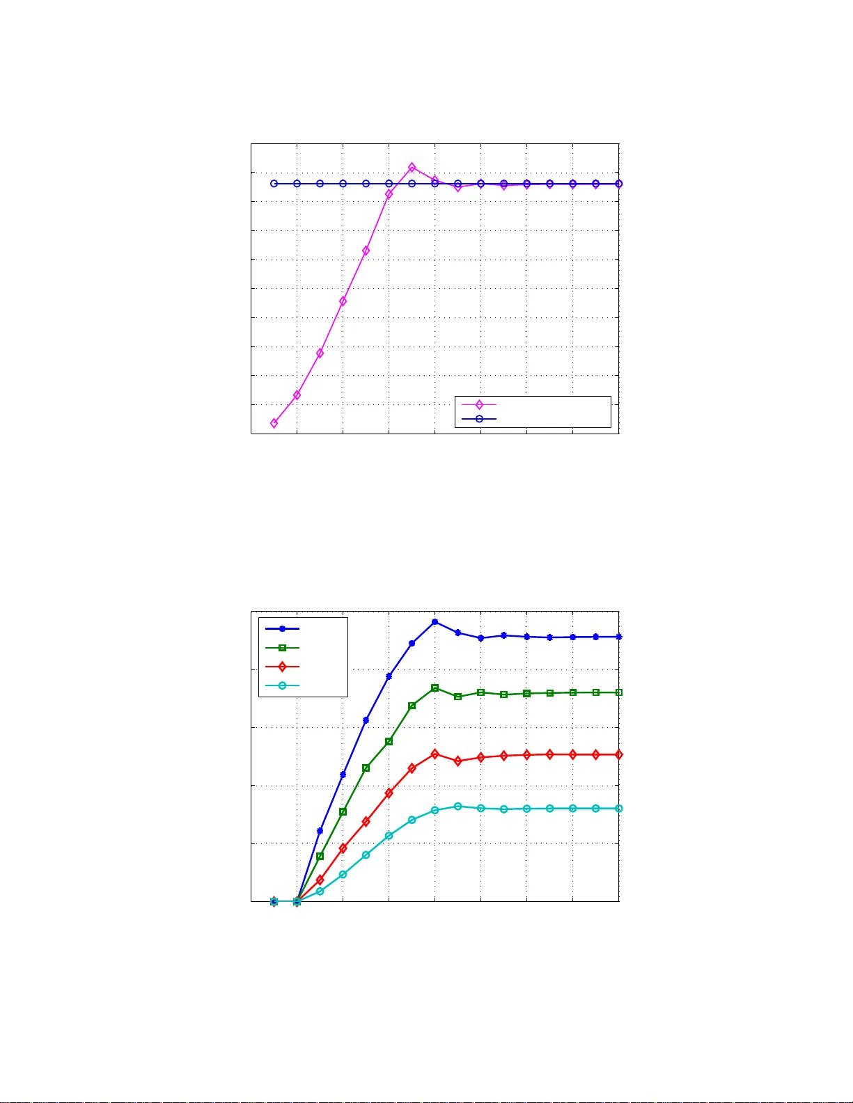
W eighted Sum Rate Optimization for Co gniti v e Radio MIMO Broadcast Channels Lan Zhang † , Y an Xin †∗ , and Y ing-Chang Liang ‡ Abstract In this paper, we consider a cogn iti ve radio (CR) ne twork in wh ich the unlicensed (second ary) users are allo wed to concurrently access th e spectru m allocated to th e licensed (prim ary) users pr ovided that their interferen ce to th e prim ary users (PUs) satisfies certain co nstraints. W e study a weighted sum rate max imization pr oblem fo r the second ary user (SU) mu ltiple inp ut mu ltiple ou tput (MIM O) broadc ast chann el (BC), in which the SUs h ave not only the sum p ower con straint but also interfe rence constraints. W e first transform this multi-constraint maximization problem into its equi valent form, which in volves a single c onstraint with multip le au xiliary variables. Fixing these multiple aux iliary v ariables, we pro pose a du ality result fo r the equ iv alen t problem. Our du ality result can solve the op timization problem f or MIM O-BC with multiple linear constrain ts, and thus can be viewed as an extension of the conv entional resu lts, which rely crucially on a single sum p ower co nstraint. Furthermor e, we develop an efficient sub-grad ient based iterati ve algor ithm to solve the equivalent problem and show that the developed algo rithm con verges to a glo bally optimal solutio n. Simulation results are fur ther provided to corr obora te the effecti veness o f the pro posed algorithm. Index T erms Beamformin g, b roadcast channel, cognitive radio , MIMO, power allo cation, sum rate m aximization. EDICS SPC-APP L: Applications in volving signal processing for communications MSP-MUL T : MIMO multi-user and multi-access schemes † The authors are with the Department of Electrical and Computer E ngineering, National Univ ersi ty of Singapore, Singapore 118622 (email: zhanglan@nus.edu.sg; elex y@nus.edu.sg). The correspon ding author of the paper is Dr . Y an Xi n (T el. no: (65) 6516-551 3 and Fax no. ( 65) 6779-11 03). ‡ The author is with Institute of Infocomm Research, 21 Heng Mui Ken g T errace, S ingapore 11961 3 (email: ycliang@i2r .a- star .edu.sg). Part of this work will be presented at IEEE International Conference on Communications, Beijing, China, May 2008. Nov ember 2, 2018 DRAFT 1 I . I N T R O D U C T I O N Cognitive radio (CR), as a p romising technol ogy to advocate efficient use of radio spectrum , has been a top ic of in creasing researc h interest in rece nt years [1]–[7]. CR allo ws an unlicensed (secondary) user to opp ortunisti cally or concurr ently access the spectrum initially allocated to the licensed (primary) users provided that certain prescribed con straints are satisfied, thus ha ving a potential to improve s pectral utilization efficiency . In this paper , we study a weighted sum rate maximi zation problem for the secondary user (SU) multipl e input multiple out put (MIMO) broadcast channel (BC) in a concurrent CR network, in which the SUs hav e no t only the sum power constraint but also int erference const raints. A. System Model and Pr obl em F ormulation W ith reference to Fig. 1, we consider t he K -SU MIMO-BC with N t transmit antennas and N r recei ve antennas in a CR network, where the K SUs share the s ame spectrum wi th a single primary user (PU) equ ipped wit h one transmitter and one receiver 1 . The transmit-receive si gnal model from the BS to the i th SU denoted by SU i , for i = 1 , . . . , K , can be expressed as y i = H i x + z i , (1) where y i is the N r × 1 rece ive d signal vector , H i is the N r × N t channel matrix from the BS t o the SU i , x is the N t × 1 t ransmitted signal vector , and z i is the N r × 1 Gaus sian noise vector with entries being independent identically distributed random variables (R Vs) with m ean zero and variance σ 2 . Consider h o as the N t × 1 channel gain vector between the transmitt ers of the BS and the PU. W e further assu me that H i for i = 1 , . . . , K , and h o remain constant during a transmis sion b lock and change independentl y from blo ck to block, and H i for i = 1 , . . . , K , and h o are perfectly known to the BS and SU i . This requires that the SUs can “cognit iv ely” obtain t he i nformation of its neighb oring en vironment. In practice, certain cooperation in terms of parameter feedback between the PU and the BS is needed. T o achiev e that, the protocol for the SU network can be designed as follo ws: e very frame con tains sensing s ub-frame and data transmissio n s ub-frame. Duri ng the s ensing sub-frame, BS can transm it training sequences to SUs as w ell as to t he PU s o t hat the SUs can esti mate the channel m atrix H i , and the PU can measure the vector h o . After t hat, thi s inform ation will be sent back to the BS via a feedback channel. 1 Expect for explicitly stated, we restrict our attention to a single PU case in the rest of this paper f or con venience of description. The results derived for the single PU case can be readily extended t o the multiple P U case, which is discussed in Remark 4. Nov ember 2, 2018 DRAFT 2 W e next cons ider the weighted sum rate maxim ization problem for the K -SU M IMO-BC in a CR network, sim ply called the CR MIMO-BC sum rate maximizatio n problem, which, mathematically , can b e formulated as Pr ob lem 1 (Main Pr oblem): max { Q b i } K i =1 : Q b i  0 K X i =1 w i r b i (2) subject to K X i =1 h † o Q b i h o ≤ P t , and K X i =1 tr ( Q b i ) ≤ P u , where r b i is the rate achiev ed by SU i , w i is the weight of SU i , Q b i denotes the N t × N t transmit signal covar iance matrix for SU i , Q b i  0 denotes t hat Q b i is a s emidefinite m atrix, P t denotes the interference threshol d of the PU, and P u denotes the su m power constraint at the BS. In a non- CR setting, s imilar weighted sum rate o ptimization problems for the m ultiple input singl e output (MISO) BC and the MIMO-BC hav e been studied in [8] [9], respectiv ely . The key d iff erence is that in addition to the sum power constraint, an interference constraint is appli ed t o the SUs in the CR MIMO-BC, i.e., the t otal receiv ed interference power P K i =1 h † o Q b i h o at the PU is below the threshold P t . Remark 1: It has l ong been observed that the opti mal sum rate for MIMO BC with a single sum p ower constraint is equal to the optimal s um rate of the dual MIMO multipl e access channel (MA C) wi th the same s um power const raint [10] [11] [12]. Ho we ver , this con ventional BC-MA C duality can on ly be applied to th e case with a singl e sum power constraint (even n ot applicabl e to an arbitrary linear p ower constraint). Hence, the additi onal interference powe r constraint in Problem 1 makes the e xisting duality cannot be applied. The new dualit y resul t p roposed in th is paper generalizes the previous resul ts as special cases. Moreover , it is worth to note that any boundary poin t of the capacity re gions of the MIMO-MA C and the MIMO-BC can be e xpressed as a weighted sum rate for a certain choice of weights [13] [14]. Thus, by varying the weight s of the SUs in Problem 1, the entire capacity region of th e CR M IMO-BC can be obtained. B. Related W o rk The present paper is m otiv ated by the previous work on the information-theoretic stud y of the MIMO-BC under a non-CR setting. It has been sh own in [11] [12] [15] that under a single sum power constraint , the sum-capacity of the non-CR MIMO-BC can be achie ved by the dirty paper coding (DPC) scheme. Furth ermore, t he paper [16 ] shows that the rate region achieved by the DPC scheme i s indeed t he capacity region of such a channel. Howe ver , t he power allocation and Nov ember 2, 2018 DRAFT 3 beamforming strategies to achie ve the capacity re gion ha ve been not considered in thes e papers. Moreover , it has been shown in [17] [18] that under the sin gle sum power constraint, the equally weighted sum rate maximi zation problem, simply called the sum rate problem, for the MIMO-BC can be solved by solv ing its dual MIMO MAC sum rate problem , which is also subject t o a sing le sum po wer constraint. In [ 17], a c yclic coordinate a scent algorithm w as proposed to solve the dual MIMO-MA C problem while in [18] this su m-power constrain ed dual problem was decoupled into an individual-power constrained problem, which can be sol ved by usi ng an iterativ e water - filling algorithm [19]. Even t hough these alg orithms proposed in [17] [18] can solve th e sum rate optimizatio n problem for th e non-CR MIMO-BC via the MA C-BC duality , they are not applicable to the general weighted sum rate problem. In [8], a generalized it erativ e water- filling was proposed to sol ve the weighted su m rate problem for the MISO-BC where each user has a single receiv e antenna. Howe ver , t he proposed algorithm i s not appli cable to the general MIMO- BC case. Furthermore, an ef ficient algorith m was proposed to sol ve t he M IMO-BC weighted sum rate problem wit h a s ingle s um power constraint in [9]. These aforementioned resul ts are based on the con ventional BC-MA C duality , which cannot be applied to solve the weighted sum rate prob lem with mu ltiple constraints (the case of in terest in t his paper). Recently , t he paper [20 ] in vestigated a different MIMO-BC weig hted sum rate maxi mization problem wh ich is subject to per-a ntenna power con straints inst ead of th e single sum power cons traint, and establish ed a new minimax duali ty which is different from the conv entional BC-MA C duality . A Newton’ s method based algorithm was proposed to solve this mini max problem. In this paper , we con sider a more general case wh ere the po wer i s subject to m ultiple linear constraints in stead of the sum power constraint or per-antenna power constraint s, and propo se a new BC-MA C duality result to extend the con ventional duality result so that it can solve t he problem with multi ple arbi trary linear constraints. A Karush-Kuhn-T ucker (KKT) condition based algorithm is de veloped to solve the problem. C. Contr ibution Throughout the p aper , we cons ider the CR MIMO-BC weighted sum rate maxi mization problem as defined in Problem 1. A s the main contribution of this paper , our solution is summarized in the following. 1) W e prove that in the CR MIMO-BC, the m ulti-constraint weighted sum rate maximi zation problem (Problem 1) i s equiv alent t o a single-constraint weight ed sum rate maximizatio n problem with multipl e auxiliary variables. Nov ember 2, 2018 DRAFT 4 2) For the equiv alent prob lem, we establ ish a duality between the MIM O-BC and a dual MIMO-MA C when t he m ultiple auxili ary variables are fixed as cons tant. This duality is applicable to MIMO-BC with arbitrary linear power constraint, and can be viewed as an extension of the con ventional MIMO MA C-BC duality result [10] [11] [12], which i s only valid for the problem with a singl e sum power cons traint. 3) For the weighted sum rate maxi mization problem of the dual MIMO MA C, the existing iterativ e water -filli ng based algorithm [17], [18 ] is not applicable. W e propo se a new pri mal dual m ethod based it erativ e algorithm [21] to solve it. Furthermore, we propose a sub - gradient based iterative algorithm to so lve the m ain problem of the p aper , Problem 1, and show that the proposed algorithm con verges t o the globally optimal solution. D. Or gan ization and Notation The rest of the paper is o r ganized as follows. In Section II, we transform the CR MIMO-BC weighted su m rate maxim ization problem (Problem 1) int o its equiv alent form, and int roduce a MA C-BC duality between a M IMO-BC and a d ual MIMO-MA C. Section III presents an primal dual method based iterativ e algorithm to solve the du al MIMO-MA C weighted sum rate p roblem. In Section IV, a M A C-BC covariance m atrix mapping algorith m i s proposed. Section V presents the complete algorithm to s olve the CR M IMO-BC weighted sum rate maximization probl em. Section VI provides severa l simulation examples. Finally , Section VII concludes the paper . The following notations are u sed in this paper . The boldface i s used to denote matrices and vectors, ( · ) † and ( · ) T denote the conjugate t ranspose and transpose, respectively; I M denotes an M × M ident ity matri x; tr ( · ) denotes the trace of a matrix, and [ x ] + denotes max( x, 0) ; ( · ) b and ( · ) m denote the quantities associated with a broadcast channel and a multiple access channel, respectiv ely; E [ · ] deno tes the expectation operator . I I . E Q U I V A L E N C E A N D D U A L I T Y Evidently , t he MIMO-BC weighted sum rate maximi zation problem under either a non-CR or a CR s etting i s a non-con ve x optimizatio n problem and i s difficult to solve directly . Under a single sum power const raint, the weighted sum rate problem for MIM O BC can be transformed to its dual MIMO MA C probl em, which is con vex and can be solved i n an effi cient manner [8] [9]. In t he CR setting, th e problem (Problem 1) has no t only a sum po wer constraint but also an int erference const raint. The imposed m ultiple constraints render difficulty to formulate Nov ember 2, 2018 DRAFT 5 an efficiently solvable dual problem. T o overcome the diffic ulty , we first transform this multi - constrained weighted sum rate problem (Problem 1) i nto its equivalent problem which has a single const raint with m ultiple auxili ary variables, and next dev elop a duali ty between a MIMO- BC and a dual MIMO-MA C in t he case where the multiple auxiliary variables are fixed. A. An Equivalent MIMO-BC W eigh ted Sum Rate Pr oblem In the following proposit ion, we present an equiv alent form of Problem 1 (see Appendix B for the proof). Pr op osition 1: Problem 1 shares the same opti mal sol ution with Pr ob lem 2 (Equival ent Pr oblem): min q t ≥ 0 , q u ≥ 0 max { Q b i } K i =1 : Q b i  0 K X i =1 w i r b i (3) subject to q t  K X i =1 h † o Q b i h o − P t  + q u  K X i =1 tr ( Q b i ) − P u  ≤ 0 , (4) where q t and q u are the auxili ary dual variables for the respectiv e interference constraint and sum power constraint. It can be readily conclu ded from the proposit ion that the optimal soluti on to Problem 2 also satisfies P K i =1 h † o Q b i h o ≤ P t and P K i =1 tr ( Q b i ) ≤ P u simultaneous ly since i t is al so the op timal solution to Problem 1. Finding an efficiently solvable du al problem for Problem 2 directly is still diffic ult. Howe ver , as we show l ater , when q t and q u are fixed as constants, Problem 2 reduces to a simplified form, which we can solve by applyi ng the fol lowing duality result. B. CR MIMO BC-MA C Dua lity For fixed q t and q u , Problem 2 reduces to the following form Pr ob lem 3 (CR MIMO-BC): max { Q b i } K i =1 : Q b i  0 K X i =1 w i r b i (5) subject to q t K X i =1 h † o Q b i h o + q u K X i =1 tr ( Q b i ) ≤ P , (6) where P := q t P t + q u P u . Since q t and q u are fixe d, P is a constant in Problem 3. The constraint (6) i s not a single sum power const raint, and thus the duali ty result established in [17] is not applicable to Problem 3. Therefore, we formulate the following new dual MA C problem. Pr op osition 2: The dual MA C prob lem of Problem 3 is Nov ember 2, 2018 DRAFT 6 Pr ob lem 4 (CR MIMO-MAC ): max { Q m i } K i =1 : Q m i  0 K X i =1 w i r m i (7) subject to K X i =1 tr ( Q m i ) σ 2 ≤ P , (8) where r m i is th e rate achieved by the i th user of the dual MA C, Q m i is the transmit si gnal cov ariance matrix of the i th user , and the noise cov ariance at t he BS is q t h o h H o + q u I N t . Remark 2: According t o Proposition 2, for fixed q t and q u , the opti mal weighted sum rate of the dual MA C is equal to the optim al weigh ted sum rate of the prim al BC. From t he formulatio n perspectiv e, thi s duality resul t is quit e similar to the con ventional duality in [10 ] [11] [12]. Howe ver , as shown in Fig. 2, o ne t hing needs to highlight is that the noise covariance matrix of the dual MA C is a function of the auxili ary variable q t and q u , inst ead of the identity matri x [12]. This differ ence comes from the constraint (6), which i s not a sum p ower cons traint as i n [12]. Note that when q t = 0 , the duality result reduces to the con ventional BC-MA C duality in [12]. As ill ustrated in Fig. 2, Proposi tion 2 describes a weighted sum rate maxim ization problem for a dual MIMO-MA C. T o prov e the propos ition, we first examine the relation between the signal to interf er ence pl us noise ratio (SINR) regions of the MIMO-BC and the dual MIMO-MA C. Based on t his relation, we wil l show that th e achiev able rate re gions of the MIMO-BC and the dual MIMO-MA C are the sam e. In th e sequel, we first describe the d efinition of t he SINR for the MIMO-BC. It has been shown in [16] t hat the DPC is a capacity achie ving scheme. Each set of the transmit covar iance matrix d etermined by DPC scheme defines a set of transm it and receiv e beamforming vectors, and each pair of thes e transmit and receiv e beamforming vectors forms a data stream. In a beamforming perspecti ve, t he BS transmitter h a ve N t × K beamformers, u i,j , for i = 1 , · · · , K , and j = 1 , · · · , N t . Therefore, the transmit signal can be represented as x = K X i =1 N t X j =1 x i,j u i,j , where x i,j is a s calar representing the data stream transmitted in this b eamformer , and E [ x 2 i,j ] = p i,j denotes the po wer al located to t his beamformer . At SU i , the recei ve beamformer correspond- ing to u i,j is denot ed by v i,j . The transmit beamformer u i,j and the po wer p i,j can be obtained via the eigen value decomposi tion of Q b i , i.e., Q b i = U † i P i U i , where U i is a u nitary matrix, and Nov ember 2, 2018 DRAFT 7 P i is a diagonal matrix. The transmi t beamformer u i,j is the j th column of U i , and p i,j is the j th d iagonal entry of P i . W it h these not ations, we express the SINR b i,j as SINR b i,j = p i,j | u † i,j H † i v i,j | 2 P K k = i +1 P N r l =1 p k ,l | u † k ,l H † i v i,j | 2 + P N r l = j +1 p i,l | u † i,l H † i v i,j | 2 + σ 2 . (9) It can be observed from (9) that the DPC scheme is applied. This can be interpreted as follows. The signal from SU 1 is first encoded with the si gnals from other SUs b eing treated as interference. The signal from SU 2 is next encoded by using the DPC schem e. Signals from the ot her SUs will be encoded sequentially in a similar manner . For t he data streams within SU i , the data stream 1 is also encoded first while th e other data streams are t reated as the interference. The data stream 2 is encoded next. In a similar manner , the other data streams wil l b e sequentially encoded. The encoding order is assumed to be arbitrary at this moment, and the optimal encoding order of Problem 2 will be discussed in Section III. T o explore the relation of the SINR regions of the dual MA C and t he BC, we formul ate a following optimi zation problem min { Q b i } K i =1 : Q b i  0 q t K X i =1 h † o Q b i h o + q u K X i =1 tr ( Q b i ) − P subject to SINR b i,j ≥ γ i,j , (10) where γ i,j denotes t he SINR threshold of the j th data st ream within the SU i for t he BC. Note that the obj ectiv e function in (10) is a function of sign al covariance matrices and the constrain ts are SINR constraints for the K -SU MIMO-BC. It has been sh own in [20] and [22] that t he non-con vex BC s um po wer minimization problem under th e SINR constraints can be sol ved ef ficiently vi a its dual MA C problem, which i s a con vex optimization problem. By following a si milar line of thinking , t he problem in (10) can be efficiently solved vi a its dual MAC problem . Similar t o the p rimal MIMO-BC, the dual MIMO-MA C depicted in Fig. 2 consist s of K users each wi th N r transmit antennas, and on e BS with N t recei ve antennas. By transposing th e channel matrix and interchanging t he input and output signals, we obtain t he dual MIMO-MA C from the primal MIMO-BC. For the cova riance matrices Q m i of t he dual MIMO-MA C, w e apply the eigen value decom position, Q m i = V i Λ i V † i = N r X j =1 q i,j v i,j v † i,j , (11) where v i,j is the j th column of V i , and q i,j is the j th diagonal entry of Λ i . For user i , v i,j is the transmit beamformin g vector of the j th data stream, t he power allocated to the j th data Nov ember 2, 2018 DRAFT 8 stream equals q i,j , and the recei ve beamforming vector of the j th data stream at the BS is u i,j . The SINR of the dual MIMO-MA C i s gi ven by SINR m i,j = q i,j | u † i,j H † i v i,j | 2 u † i,j  P i − 1 k =1 P N r l =1 q k ,l H † k v k ,l v † k ,l H k + P j − 1 l =1 q i,l H † i v i,l v † i,l H i + R w  u i,j , (12) where R w := q t R o + q u I N t is the noise cova riance matrix of the MIMO-MA C wi th R o := h o h † o . In the dual M IMO-MA C, R w depends on q t and q u defined in (10) whereas the no ise cova riance matrix in the primal MIM O-BC is an identity matrix. It can be observed from (12) that the successiv e in terference cancelation (SIC) scheme is used in thi s dual MIMO-M A C, and the decoding order is the reve rse encoding order of t he primal BC. The signal from SU K is first decoded with the signals from other users being treated as interference. After decoded at the BS, the signals from SU K will be subtracted from the recei ved signal. The sig nal from SU K − 1 is next decoded, and so on. Again , th e data streams within a SU can be decoded in a sequenti al manner . For the dual MIMO-M A C, we consid er the follo wing m inimizatio n p roblem sim ilar to the problem (10) min { Q m i } K i =1 : Q m i  0 K X i =1 tr ( Q m i ) σ 2 − P subject to SINR m i,j ≥ γ i,j . (13) The following proposit ion describes the relation between the problems (10) and (13). Pr op osition 3: For fixed q t and q u , the MIMO-MA C problem (13) is dual to the MIMO-BC problem (10). Pr oo f: The cons traints in (10) can be re written as p i,j | u † i,j H † i v i,j | 2 γ i,j ≥ K X k = i +1 N r X l =1 p k ,l | u † k ,l H † i v i,j | 2 + N r X l = j +1 p i,l | u † i,l H † i v i,j | 2 + σ 2 . (14) Thus, the Lagrangian function of the problem (10) is L 1 ( Q b 1 , . . . , Q b K , λ i,j ) = q t K X i =1 h † o Q b i h o + q u K X i =1 tr ( Q b i ) − P − K X i =1 N r X j =1 λ i,j  p i,j | u † i,j H † i v i,j | 2 γ i,j − K X k = i +1 N r X l =1 p k ,l | u † k ,l H † i v i,j | 2 − N r X l = j +1 p i,l | u † i,l H † i v i,j | 2 − σ 2  (15) Nov ember 2, 2018 DRAFT 9 = K X i =1 N r X j =1 λ i,j σ 2 − P − K X i =1 N r X j =1 p i,j u † i,j  λ i,j H † i v i,j v † i,j H i γ i,j − i − 1 X k =1 N r X l =1 λ k ,l H † k v k ,l v † k ,l H k − j − 1 X l =1 λ i,l H † i v i,l v † i,l H i − R w  u i,j , (16) where λ i,j is the Lagrangian multipl ier . Eq. (16) is obtain ed by applying the eigen value decom- position to Q b i and rearranging the terms in (15). The optim al objective v alue of (10) is max λ i,j min Q b 1 ,..., Q b K L 1 ( Q b 1 , . . . , Q b K , λ i,j ) . (17) On the other h and, the Lagrangian function of the problem (13) is L 2 ( Q m 1 , . . . , Q m K , δ i,j ) = K X i =1 N r X j =1 q i,j σ 2 − P − K X i =1 N r X j =1 δ i,j u † i,j ( q i,j H † i v i,j v † i,j H i γ i,j − i − 1 X k =1 N r X l =1 q k ,l H † k v k ,l v † k ,l H k − j − 1 X l =1 q i,l H † i v i,l v † i,l H i − R w ) u i,j , (18) where δ i,j is the Lagrangian multi plier . Eq. (18) is also obtained by applying eig en value decom- position to Q m i . The optimal objective v alue of (13) i s max δ i,j min Q m 1 ,..., Q m K L 2 ( Q m 1 , . . . , Q m K , δ i,j ) . (19) Note that if we choose q i,j = λ i,j , δ i,j = p i,j , and the same beamforming vectors u i,j and v i,j for bot h problems, (16) and (18) become identical. T his means that the optimal solu tions of (17) and (19) are the same. Proposition 3 impl ies that under the SINR constraints, the problems (10) and (13) can achie ve the same objective value, wh ich is a function of the transm it signal cov ariance matrices. On the other hand, un der th e correspondi ng const raints on the signal cov ariance m atrix, the achiev able SINR regions of the MIMO-BC and its dual MIMO-MA C are the same. Mathematically , we define the respecti ve achiev able SINR regions for the primal MIMO-BC and the dual MIMO- MA C as fol lows. Definition 1: A SINR vector γ = ( γ 1 , 1 , . . . , γ 1 ,N t , . . . , γ K,N t ) is said to be achieva ble for the prim al BC if and only if th ere exists a set of Q b 1 , . . . , Q b K such that q t P K i =1 h † o Q b i h o + q u P K i =1 tr ( Q b i ) − P ≤ C for a const ant C and the correspondi ng SINR b i,j ≥ γ i,j . An achie vable BC SINR region deno ted by R B C , is a set containing all the BC achie vable γ . Definition 2: A SINR vector γ = ( γ 1 , 1 , . . . , γ 1 ,N t , . . . , γ K,N t ) is s aid to b e achiev able for the dual MA C if and only if there exists a set of Q m 1 , . . . , Q m K such that P K i =1 tr ( Q m i ) σ 2 − P ≤ C for Nov ember 2, 2018 DRAFT 10 a cons tant C and the correspondi ng SINR m i,j ≥ γ i,j . An achiev able MA C SINR region denoted by R M AC , is a set containing all the MA C achiev able γ . In t he following corollary , we will show R M AC = R B C . Cor oll ary 1: For fixed q t and q u , and a constant C , the MIMO-BC under the constraint q t P K i =1 h † o Q b i h o + q u P K i =1 tr ( Q b i ) − P ≤ C and the du al MIM O-MA C under the cons traint P K i =1 tr ( Q m i ) σ 2 − P ≤ C achiev e t he sam e SINR region. Pr oo f: For any γ ∈ R M AC , b y Definition 2, there exists a set of Q m 1 , . . . , Q m K such that P K i =1 tr ( Q m i ) σ 2 − P ≤ C and the corresponding SINR m i,j ≥ γ i,j . It can be readily concluded from Proposition 3 that there exists a set of Q b 1 , . . . , Q b K such t hat q t P K i =1 h † o Q b i h o + q u P K i =1 tr ( Q b i ) − P ≤ C and the corresponding SINR b i,j ≥ γ i,j . This im plies γ ∈ R B C . Since γ i s an arbitrary element in R MA C , we ha ve R M AC ⊆ R B C . In a similar manner , we have R B C ⊆ R M AC . The proof follows. W e are now in the position to prove Proposition 2. Pr oo f of Pr op osition 2: According to Corollary 1, if C = 0 , then under the constraint q t P K i =1 h † o Q b i h o + q u P K i =1 tr ( Q b i ) ≤ P for t he BC and the constraint P K i =1 tr ( Q m i ) σ 2 ≤ P for the dual MA C, the two channels ha ve the s ame SINR region. Since the achie v able rates of us er i in the MIMO-MA C and th e MIMO -BC are r m i = P N r j =1 log(1 + SINR m i,j ) and r b i = P N r j =1 log(1 + SINR b i,j ) , t he rate regions of the two channels are the same. Therefore, Proposition 2 follows.  Note that due to the additional interference constraint , Problem 2 cannot be so lved by using the established duality result in [11] and [12], in which only a single sum power constraint w as considered. Our duality resul t in Proposition 2 can be t hought as an e xtension of the dualit y results in [11] [12] to a multip le li near const raint case. Moreover , as will be sh own in the following section, our duality result formu lates a M IMO-MA C problem (Problem 4), which can be ef ficiently solved. I I I . D UA L M AC W E I G H T E D S U M R A T E M A X I M I Z A T I O N P R O B L E M In this section , we propose an efficient algorithm to s olve Problem 4. W i th the SIC scheme, the achiev able rate of the k th user i n the dual MIMO-MA C is given by r m k = log | R w + P k j =1 H j Q m j H † j | | R w + P k − 1 j =1 H j Q m j H † j | . (20) For the MIMO-MAC , the equally weighted sum rate m aximization is irrespective of the decoding order . Ho wev er , i n general the weigh ted sum rate maxim ization in the MIMO-MA C is affec ted Nov ember 2, 2018 DRAFT 11 by the decodi ng order . W e thus need to consider the opti mal decoding order of the SIC for the dual MIMO-M A C, and further need to consider the corresponding optimal encoding order of the DPC for the primal BC. Let π be the optimal decoding order , which is a permutation on the SU index s et { 1 , · · · , K } . It follows from [14] that the optimal user decoding order π for Problem 4 is the order such that w π (1) ≥ w π (2) ≥ · · · ≥ w π ( K ) is sati sfied. Th e following lemma presents the opt imal decoding order of the SIC for the data streams within a SU (see Appendix C for the proof). Lemma 1: T he op timal data stream decoding order for a particular SU is arbitrary . Due to the du ality betw een the MIMO-BC and the MIMO-MA C, for Problem 3, the opt imal encoding order for the DPC i s the reve rse of π . Because of the arbitrary encoding order for the data s treams within a SU, if we choo se a different encoding order for the BC, the MA C-to-BC mapping algorithm can give differ ent results whi ch y ield th e same objective va lue. Hence, the matrix Q b i achie ving the optimal objectiv e value are not unique. W i th no l oss of generalit y , we assume w 1 ≥ w 2 ≥ · · · ≥ w K for notational con venience. According to (2 0), the objective function of Problem 4 can be re written as f ( Q m 1 , · · · , Q m K ) := K X i =1 ∆ i log | R w + i X j =1 H j Q m j H † j | , (21) where ∆ i := w i − w i +1 , and w K +1 := 0 . Clearly , Problem 4 is a con vex p roblem, which can be solved through standard con vex optimization soft ware packages directly . Howe ver , the standard con vex optimization software does n ot exploit the special structure of the probl em, and t hus is computationall y expensive . An efficient algorithm was dev eloped to sol ve a weighted su m rate maximization problem for the SIMO-MA C in [8]. Howev er , since t his algorithm just consider the case where each us ers h as a single data st ream, i t is not applicable to our probl em. In the following, we dev elop a prim al dual method based algorithm [21] to solve this problem. W e next rewrite Problem 4 as max { Q m i } K i =1 : Q m i  0 f ( Q m 1 , · · · , Q m K ) subject to K X i =1 tr ( Q m i ) ≤ P . (22) Recall that t he posit iv e semi-definiteness of Q m i is equiv alent to the po sitiveness of the eigen- values of Q m i , i.e., q i,j ≥ 0 . Correspondin gly , the Lagrangian function is L ( Q m 1 , · · · , Q m K , λ, δ i,j ) = f ( Q m 1 , · · · , Q m K ) − λ  K X i =1 tr ( Q m i ) − P  + K X i =1 M i X j =1 δ i,j q i,j , (23) Nov ember 2, 2018 DRAFT 12 where λ and δ i,j are Lagrangian multi pliers. According to the KKT conditi ons of (22), we ha ve ∂ f ( Q m 1 , · · · , Q m K ) ∂ Q m i − λ I N r + M i X j =1 δ i,j E i,j = 0 , (24) λ  K X i =1 tr ( Q m i ) − P  = 0 , (25) δ i,j q i,j = 0 , (26) where E i,j := ∂ q i,j /∂ Q m i . Notice that it is not necessary to compute th e actual v alue of δ i,j and E i,j , because if δ i,j 6 = 0 , then q i,j = 0 . Thus, the semi-definite constraint tu rns into q i,j = [ q i,j ] + . Thus, we can assume δ i,j = 0 . The d ual objective function o f (22) is g ( λ ) = max { Q m i } K i =1 : Q m i ≥ 0 L ( Q m 1 , · · · , Q m K , λ ) . (27) Because the problem (22) is con ve x, it is equivalent to t he following minimizatio n problem min λ g ( λ ) subject to λ ≥ 0 . (28) W e outline the algorith m to solve the problem (28). W e choose an initial λ and compute the value of g ( λ ) (27), and then up date λ according to the descent direction of g ( λ ) . The process repeats until the algorithm con ver ges. It is easy to o bserve that all the users share the s ame λ , and thus λ can be viewed as a water lev el in the water filling principle. Once λ is fixe d, the uniq ue optimal set { Q m 1 , . . . , Q m K } can be obtained through th e gradi ent ascent alg orithm. In each iterative step, Q m i is updated s equentially according to its gradient d irection of (23). Denote by Q m i ( n ) the matrix Q m i at the n th iteration step. The gradient of each step is determined by ∇ ( n ) Q m i L := ∂ f  Q m 1 ( n ) , · · · , Q m i − 1 ( n ) , Q m i ( n − 1) , . . . , Q m K ( n − 1)  ∂ Q m i ( n − 1) − λ I N r . (29) Thus, Q m i ( n ) can be updated according to Q m i ( n ) = h Q m i ( n − 1) + t ∇ ( n ) Q m k L i + , where t is the step size, and the n otation [ A ] + is defined as [ A ] + := P j [ λ j ] + v j v † j with λ j and v j being the j th eigen value and the correspond ing eigen vector of A respectively . The gradient in (29) can be readily computed as ∂ f ( Q m 1 , · · · , Q m K ) ∂ Q m k = K X j = k ∆ j  H k F j ( Q m 1 , · · · , Q m K ) − 1 H † k  , (30) Nov ember 2, 2018 DRAFT 13 where F j ( Q m 1 , · · · , Q m K ) := R w + P j i =1 H † i Q m i H i . W e next need to determin e the optim al λ . Since the Lagrangian function g ( λ ) i s con ve x over λ , the optimal λ can be obtained through the one-dimensional search. Howe ver , because g ( λ ) is not n ecessarily diffe rentiable, the gradient algorithm cannot be appli ed. Alternati vely , the subgradient method can be used to find the opt imal solution. In each iterativ e step, λ is updated according to the subgradient direction. Lemma 2: T he sub-gradient o f g ( λ ) is P − P K i =1 tr ( Q m i ) , where λ ≥ 0 , and Q m i , i = 1 , . . . , K , are the corresponding optimal cov ariance m atrices for a fixed λ in (27). Pr oo f: The proo f is provided in Appendix D. Lemma 2 indicates that the value of λ should increase, if P K i =1 tr ( Q m i ) > P , and vice versa. W e are now ready to present our algorithm for solving Problem 4. Decoupled Iterative P ower Allocati on (DIP A) Algorithm : 1) Initialize λ min and λ max ; 2) repeat a) λ = ( λ min + λ max ) / 2 b) repeat, initialize Q m 1 (0) , · · · , Q m K (0) , n = 1 for i = 1 , · · · , K Q m i ( n ) = h Q m i ( n − 1) + t ∇ ( n ) Q m i L i + , end for n = n + 1 , c) until Q m k for k = 1 , · · · , K con verge, i.e., k∇ ( n ) Q m i L k 2 ≤ ˆ ǫ for a small preset ˆ ǫ . d) if P K i =1 tr ( Q m i ) > P , then λ min = λ , el seif P K i =1 tr ( Q m i ) < P , t hen λ max = λ ; 3) until | λ min − λ max | ≤ ǫ , where ǫ > 0 is a constant. Th e following proposit ion sho ws the con ver gence prop erty of the DIP A alg orithm. Pr op osition 4: The DIP A algorithm con ver ges t o an opt imal set of the MA C transm it signal cov ariance matrices. Pr oo f: The DIP A algorithm consists of th e inner and outer loops. The inner loop is to compute Q m i for i = 1 , · · · , K . In each iterativ e step of the inner loop, we update Q m i by fixing other Q m j with j 6 = i , and compute the corresponding gradient. The inner loop uses the gradient ascent alg orithm, which con ver ges to the o ptimal value due to its nond ecreasing property and the con vexity of the objecti ve functio n. The o uter loop is to compute the optimal Lagrangian multipli er λ in (28). Due to the conv exity of the dual objectiv e function [23], there is a unique λ achieving the o ptimal solu tion in (28). Hence, we can use an effic ient one dimens ional line Nov ember 2, 2018 DRAFT 14 bisection search ( [19], [18]). Remark 3: In the previous work on th e sum rate maximizatio n [19] [17] [18], th e cov ariance matrix of each user is the same as the singl e us er water -filli ng cov ariance m atrix in a po int-to- point li nk with m ultiuser in terference bei ng t reated as nois e [24]. Howe ver , for t he weigh ted su m rate maxi mization problem, the optimal s olution does not possess a water -filli ng structure. Thus, our DIP A algorithm do es not ob ey the water- filling princip le. In Section VI, Example 1 compares the water- filling algorithm with the DIP A algorithm. Not ably , the formulation of Problem 4 i s similar to the weighted sum rate problem for the dual MIMO M A C in [9]. The a lgorithm proposed therein to handle the dual MIMO MA C prob lem is b ased on gradient projection meth od [21]. The difference between our DIP A algorithm and the alg orithm in [9] is just li ke t he difference between the algorithms in [17] and [18]. The DIP A algorithm is an efficient algorithm to obtain the o ptimal t ransmit covariance matrix of the d ual M IMO M A C (Problem 4). Moreover , the optimal solution to Problem 3 can be obtained via t he MA C-to-BC cov ariance matrix mapping algorithm p resented in t he n ext section. I V . M AC - T O - B C C OV A R I A N C E M A T R I X M A P P I N G A covariance matrix mappi ng algorit hm was d e veloped in [12]. Howe ver , this algorithm works for the sum rate m aximization problem under a singl e sum power c onstraint, and is no t applicable to a weigh ted sum rate problem under multi ple constraints. In the following, we develop a cov ariance matrix mapping algori thm, which computes t he BC covariance m atrices Q b i via the dual MA C covariance matrices Q m i such that two channels yield a same weighted sum rate. In the MIM O-MA C, acc ording to (11), the transmit beamforming vectors v i,j can be obtained by the eig en value decomp osition. The corresponding receive beamforming vector at th e BS, u i,j , is obtained by using the minimum mean square error (MMSE) algorithm: u i,j = a  i − 1 X k =1 N r X l =1 q k ,l H † k v k ,l v † k ,l H k + j − 1 X l =1 q i,l H † i v i,l v † i,l H i + R w  − 1 H † i v i,j , (31) where a is a normalized fa ctor such that || u i,j || = 1 . Throughout the proof of Proposition 3, we can see that when the same optimal solutions are achie ved the primal BC and the dual MA C share the same beamforming vectors u i,j and v i,j . Hence, the t ransmit beamforming vectors of the BC are just th e recei ve beamforming vectors of th e dual MAC , and t he receiv e beamforming vectors of t he BC are the transmit beamformi ng vectors of t he du al MA C. Thu s, to obtain the transmit signal covar iance matrix of SU i for the BC, we onl y need to comp ute the power allocated to each data stream. Due to Corollary 1, the dual MA C and the BC can achieve the same SINR region, Nov ember 2, 2018 DRAFT 15 i.e., SINR b i,j = SINR m i,j . Th us, fo r the BC, the power allocated to t he beamform ing direction u i.j can be obtained by p i,j = SINR m i,j  P K k = i +1 P N r l =1 p k ,l | u † k ,l H † i v i,j | 2 + P N r l = j +1 p i,l | u † i,l H † i v i,j | 2 + σ 2  | u H i,j H † i v i,j | 2 . (32) For the BC, the encoding order is the reverse of the decoding order of t he M A C. Thus, p K,N r is comp uted first, p K,N r − 1 is comp uted second, and so on, in the decreasing order of t he d ata stream index and the us er in dex. After comput ing the power for al l the beamfo rming vectors, we obtain t he signal covari- ance matrix from the BS to SU i , Q b i = P N r j =1 p i,j u i,j u † i,j . Th e aforedescribed process can be summarized as the following algorithm. MA C-to-BC Cov ariance Matri x Map ping Algorithm: 1) Compute q i,j and v i,j through eigen value decomp osition: Q m i = V i Λ i V † i = P N r j =1 q i,j v i,j v † i,j ; 2) Use t he MMSE algorit hm to obtain the optimal receiver beamforming vector u i,j and SINR m i,j ; 3) Compute p i,j through (32) according to the duality between the BC and the MA C; 4) Compute Q b i = P N r j =1 p i,j u i,j u † i,j . It shoul d be noted t hat even though an explicit algo rithm is no t given, the paper [20] has mentioned the idea behin d the above algorithm . The M A C-to-BC cov ariance matrix mappi ng allows us to obtain the optimal BC cov ariance m atrices for Problem 3 by solving Problem 4. V . A C O M P L E T E S O L U T I O N T O T H E CR M I M O - B C W E I G H T E D S U M R A T E P RO B L E M W e are now ready to present a complete algo rithm to so lve Problem 2. The Lagrangian dual objective function of Problem 2 can be rewritten as follows g ( q t , q u ) = max { Q b i } K i =1 : Q b i  0 K X i =1 w i r b i , (33) where the maximizati on is subject t o t he constraint q t  P K i =1 h † o Q b i h o − P t  + q u  P K i =1 tr ( Q b i ) − P u  ≤ 0 . Problem 2 is equiv al ent to the following probl em min q t ,q u g ( q t , q u ) , s ubject to q t ≥ 0 and q u ≥ 0 . Applying the BC-MA C du ality in Section II-B and t he DIP A algorithm in Section III, g ( q t , q u ) can be obtained. The remainin g task is to determine the optimal q t and q u . Since g ( q t , q u ) is not necessarily differ entiable, we search the optim al q t and q u through the subgradient algorithm ; Nov ember 2, 2018 DRAFT 16 that is, i n each iterati ve step, we update th e ve ctor [ q t , q u ] according to the sub gradient d irection s = [ s 1 , s 2 ] of g ( q t , q u ) . Lemma 3: T he subgradient of g ( q t , q u ) is  P t − P K i =1 h † o Q b i h o , P u − P K i =1 tr ( Q b i )  , where q t ≥ 0 , q u ≥ 0 , and Q b i , i = 1 , . . . , K , are the corresponding op timal cov ariance matrices for the problem (33). Pr oo f: The proo f is giv en in Appendi x E. It has been shown in [25] that with a constant step size, t he subgradient alg orithm con ver ges to a v alue that is within a small range of the optimal value, i.e., lim n →∞ | q ( n ) t − q ∗ t | < ǫ, and , lim n →∞ | q ( n ) u − q ∗ u | < ǫ, (34) where q ∗ t and q ∗ u denote the o ptimal values, and q ( n ) t and q ( n ) u denote the values of q t and q u at the n th step of the subgradient algorithm, respectively . This implies that the subgradient m ethod finds an ǫ -subopt imal point within a finite number of steps. The nu mber ǫ is a decreasing functi on of the step s ize. Moreover , if the dimini shing step size rule, e.g., the square summ able b ut no t summable step size, is applied, the algorithm is guaranteed to con verge to th e opt imal value. W e next describe the algorithm to solve Problem 2 as follows. Subgradient Iterative P ower A llocation (SIP A) A lgorithm : 1) Initialization: q (1) t , q (1) u , n = 1 , 2) repeat 2a) Find the op timal s olution of the dual MA C Problem 4 through the DIP A alg orithm; 2b) Find t he so lution of the BC problem (33) through the MA C-to-BC m apping algo rithm; 2c) Up date q ( n ) t and q ( n ) u through a subgradi ent algorithm q ( n +1) t = q ( n ) t + t ( P K i =1 h † o Q b i h o − P t ) , q ( n +1) u = q ( n ) u + t ( P K i =1 tr ( Q b i ) − P u ) , 2d) n = n + 1 3) Stop when | q ( n ) t ( P K i =1 h † o Q b i h o − P t ) | ≤ ǫ and | q ( n ) u ( P K i =1 tr ( Q b i ) − P u ) | ≤ ǫ are satisfied simultaneous ly , where t denotes the st ep size of the subgradient algorithm. As a sum mary , the flow chart of the SIP A algorithm is depi cted in Fig. 3. W e shows that the SIP A algorithm con verges to the optimal solution of Problem 1 in the following propositi on. Pr op osition 5: The SIP A algorith m con verges to the gl obally o ptimal solution of Problem 1. Pr oo f: The Lagrangian function of Problem 1 is giv en b y L ( Q b 1 , . . . , Q b K , λ 1 , λ 2 ) = K X i =1 w i r b i − λ 1  K X i =1 h † o Q b i h o − P t  − λ 2  K X i =1 tr ( Q b i ) − P u  , (35) Nov ember 2, 2018 DRAFT 17 and the Lagrangian function of Problem 2 is giv en by L 1 ( Q b 1 , . . . , Q b K , λ, q t , q u ) = K X i =1 w i r b i − λ  q t  K X i =1 h † o Q b i h o − P t  − q u  K X i =1 tr ( Q b i ) − P u  . (36) Let ¯ q t , ¯ q u , ¯ λ , and ¯ Q i be t he op timal v alues of L 1 ( Q b 1 , . . . , Q b K , λ, q t , q u ) , when the alg orithm con verges. W e thus have ∂ L 1 ( Q b 1 , . . . , Q b K , λ, q t , q u ) ∂ Q b i    { ¯ Q b i } K i =1 , ¯ λ, ¯ q t , ¯ q u = 0 , | ¯ q t ( P K i =1 h † o ¯ Q i h o − P t ) | = 0 , and | ¯ q u ( P K i =1 tr ( ¯ Q i ) − P u ) | = 0 . This means that ¯ Q i is a locally optimal solution. According to (35), if we select ˜ λ 1 = ¯ λ ¯ q t , ˜ λ 2 = ¯ λ ¯ q u , and ˜ Q i = ¯ Q i , then ˜ λ 1 , ˜ λ 2 , and ˜ Q i satisfy the KKT conditions of Problem 1 and thus are the locally optimal va riables. Suppose that there exists an o ptimal set of ˆ λ 1 , ˆ λ 2 , and ˆ Q i such that L ( ˆ Q 1 , . . . , ˆ Q K , ˆ λ 1 , ˆ λ 2 ) > L ( ˜ Q 1 , . . . , ˜ Q K , ˜ λ 1 , ˜ λ 2 ) . Clearly , this op timal set of ˆ λ 1 , ˆ λ 2 , and ˆ Q i satisfy t he KKT condi tions of Problem 1. In the sequel, we will deriv e a contradiction. First, we can write L ( ˜ Q 1 , · · · , ˜ Q K , ˜ λ 1 , ˜ λ 2 ) ≥ L ( ˆ Q 1 , · · · , ˆ Q K , ˜ λ 1 , ˜ λ 2 ) . (37) Suppose that (37) does not hol d, i.e., L ( ˜ Q 1 , · · · , ˜ Q K , ˜ λ 1 , ˜ λ 2 ) < L ( ˆ Q 1 , · · · , ˆ Q K , ˜ λ 1 , ˜ λ 2 ) . Then, according to the BC-MA C duality in Se ction II-B, an o bjectiv e value of (7) which is larger than L ( ˜ Q 1 , · · · , ˜ Q K , ˜ λ 1 , ˜ λ 2 ) , can be found for th e fixed ¯ q t and ¯ q u . H owe ver , from Propositi on 4, the DIP A alg orithm con ver ges the opti mal sol ution. It is a contradiction. Secondly , according to the KKT conditi ons of Problem 1, we have ˆ λ 1  K X i =1 h † o ˆ Q b i h o − P t  = 0 , (38) ˆ λ 2  K X i =1 tr ( ˆ Q b i ) − P u  = 0 . (39) W e thus can write: L ( ˆ Q 1 , · · · , ˆ Q K , ˜ λ 1 , ˜ λ 2 ) ≥ L ( ˆ Q 1 , · · · , ˆ Q K , ˆ λ 1 , ˆ λ 2 ) . (40) Combining (40) and (37), we hav e L ( ˜ Q 1 , · · · , ˜ Q K , ˜ λ 1 , ˜ λ 2 ) ≥ L ( ˆ Q 1 , · · · , ˆ Q K , ˆ λ 1 , ˆ λ 2 ) . (41) This contradicts with our previous assumptio n. Nov ember 2, 2018 DRAFT 18 Remark 4: The algo rithm can be extended to the multi ple PU case i n the following manner . Assume that there are N PUs. Problem 2 becom es min q t,j ≥ 0 ,q u ≥ 0 max { Q b i } K i =1 : Q b i  0 K X i =1 w i r b i , subject to N X j =1 q t,j  K X i =1 h † o,j Q b i h o,j − P t,j  + q u  K X i =1 tr ( Q b i ) − P u  ≤ 0 , (42) where q t,j is the auxili ary va riable for th e j th PU, h o,j is the channel response from the BS t o the j th PU, and P t,j is the interference threshold of the j th PU. The role of auxili ary variables q t,j is si milar to that of q t in th e single PU case. It is thus straightforward to mo dify the SIP A algorithm to solve t he problem for the multi ple PU case. Moreover , it should be noted that the multiple interference constrain ts of the problem (42) can b e transformed to the per-antenna power constraints [20] by setting h o,j , j = 1 , · · · , N t , to be th e j th colum n of the identity matrix . Not limited by the su m rate maximizati on problem with interference power const raints, the method proposed in this paper can be easily app lied to s olve the transmitter optimization problem (e.g. beamforming optimi zation) for MIMO BC with multip le arbitrary linear power const raints. V I . S I M U L A T I O N R E S U L T S In t his section, we provide the si mulation result s to show the effecti veness of the proposed algorithm. In t he simulations , for simpl icity , we assume that t he BS is at the same dis tance, l 1 , to all SUs, and the same distance, l ( n ) 2 , to PU n . In the single PU case, we will drop the superscript and simply use notation l 2 . Suppose that the s ame p ath loss model can be used t o describe the transmissio ns from the BS to the SUs and to the PUs, and th e pass loss exponent is 4. The elements of matrix H are assumed to be circularly sym metric com plex Gaussi an (CSCG) R Vs with mean zero and variance 1, and h o can be modeled as h o = ( l 1 /l 2 ) 2 a n , where a n is a N t × 1 vector whose elements are CSCG R Vs with mean zero and variance 1. The noise covariance matrix at the BS is assumed to be t he identit y m atrix, and the sum power and i nterference power are defined in dB relative to the noise power , and P t is chosen to be 0 dB. F or all cases, we choose l 1 = l 2 , except for explicitly stated. Example 1: In Fig. 4, we examine the v alidity of the DIP A algorithm . In this example, we choose K = 1 (a single SU case), N t = 4 , N r = 4 , and P u = 10 dB. It is wel l known that the optimal transm it sign al covariance matrix can be obtained through the water -filling principle [24]. As can be observed from Fig. 4, in se veral i terations, the DIP A algorithm con ver ges to t he optimal solution obtained by using the water -filling principle. Nov ember 2, 2018 DRAFT 19 Example 2: In Fig. 5, we show the con ver gence property o f the DIP A algo rithm. In thi s example, we choos e K = 2 0 and P u = 10 dB. It can be observed from this figure that the algorithm con verges to the opti mal sol ution within se veral iteration steps . Example 3: In Figs. 6 and 7, we consid er a SU MIMO -BC network with K = 5 , N t = 5 , N r = 3 , and P u = 13 dB. In t his example, the SUs wit h w 1 = 5 and w i = 1 , i = 2 , . . . , K are assumed to share the same spectrum band with two PUs. Fig. 6 plots the weighted sum rate versus th e nu mber of iteration s of the SIP A algorithm for step sizes t = 0 . 1 and t = 0 . 01 . As can be seen from the figure, the step size af fects the accurac y and con ver gence speed of the algorithm. Fig. 7 plots the sum power at the BS and t he i nterference power at the PUs versus the number of it erations. It can be seen from th e figure that the sum power and the interference power approach to P u = 13 dB and P t = 0 dB respectiv ely when the SIP A alg orithm con ver g es. This impl ies that the sum power and interference constraints are satisfied with equalit ies when the SIP A alg orithm con verges. Example 4: Fig. 8 plots t he achiev able s um rates versus the sum po wer in the single PU case and the case wi th no PU. W e choose K = 5 , N t = 5 , and N r = 3 . As can be seen from Fig. 8, in the low sum power regime, the achiev able sum rate in the case with no PU is quite close to th e one in th e single PU case while i n the hi gh sum power regime, t he achiev able sum rate in the case with no PU is much higher than th e one in the single PU case. T his is because the additional constraint reduces the degrees of freedom of the sy stem. Example 5: In this example, we consider the influence o f th e interference cons traint on the achie vable sum rate of the SUs. In this example, N t = 5 , K = 5 , and N r = 3 . The sum power constraint for the BS is assumed to be 15 dB and 20 dB. Fig. 9 compares the sum rate achie ved in a PU case wi th one achieved i n the case with no PU as l 2 /l 1 var ies from 1 to 12. It can be observed from the figure that the achiev able sum rate in creases as the PU m oves aw ay from the BS, and the influence o f the PU reduces to zero after the l 2 /l 1 is lar ger than a certain thresho ld. V I I . C O N C L U S I O N S In this paper , we de veloped a new BC-MA C duality result, which can be viewed as a n extension of existing du al results d e veloped un der either a sum po wer constraint or per -antenna power constraints. Exploitin g this d uality result, we proposed an efficient algorithm to solve the CR MIMO-BC weig hted su m rate maxi mization problem . W e further showed that the proposed algorithm con verges to the glob ally opt imal solution. Nov ember 2, 2018 DRAFT 20 A P P E N D I X A. Lemma 4 and it s pr oof: The following lemma describes an important property that will be used in the proof of other lemmas. Lemma 4: For fixed q t and q u , the maximum weighted sum rate in (5) i s achie ved when the constraint (6) is satisfied with equality . Pr oo f: W e here adopt the DPC scheme, which is a capacity achieving strategy for the MIMO-BC [16]. Let the permut ation π represent the encoding order when the o ptimal solu tion is achie ved. Assume t hat SU π (1) is encoded first such that the signal of SU π (1) is noncausally known to the BS before the signals from the other SUs are encoded. Th us, in the DPC schem e the signal from SU π (1) has no i mpact on the rates achiev ed by the other SUs. W e prove this lemma by contradiction. Suppose that Q b π (1) is the op timal signal cova riance matrix of SU π (1) . Assume that the con- straint (6) is satisfied with a strict inequality when the op timal solut ion is achie ved. Thus, we can alwa ys find an ǫ > 0 such that q t  K X i =2 h † o ( Q b π ( i ) ) h o + h † o ( Q b π (1) + ǫ I ) h o − P t  + q u  K X i =2 tr ( Q b π ( i ) ) + tr ( Q b π (1) + ǫ I ) − P u  = q t  K X i =1 h † o ( Q b π ( i ) ) h o + h † o ( ǫ I ) h o − P t  + q u  K X i =1 tr ( Q b π ( i ) ) + tr ( ǫ I ) − P u  < 0 . (43) Moreover , the rate achiev ed by user π (1 ) in the MIMO-BC can be wri tten as r b π (1) = log    I + P K i =1 H π (1) Q b π ( i ) H † π (1)       I + P K i =2 H π (1) Q b π ( i ) H † π (1)    . Due to the positive semi-definiteness prop erty o f Q b i , we hav e log    I + K X i =2 H π (1) Q b π ( i ) H † π (1) + H π (1) ( Q b π (1) + ǫ I ) H † π (1)    = log    I + K X i =2 H π (1) Q b π ( i ) H † π (1)    + log    I + ( I + K X i =2 H π (1) Q b π ( i ) H † π (1) ) − 1 / 2 H π (1) ( Q b π (1) + ǫ I ) H † π (1) ( I + K X i =2 H π (1) Q b π ( i ) H † π (1) ) − 1 / 2    Nov ember 2, 2018 DRAFT 21 = log    I + K X i =2 H π (1) Q b π ( i ) H † π (1)    + log    I + G † ( Q b π (1) + ǫ I ) G    = log    I + K X i =2 H π (1) Q b π ( i ) H † π (1)    + log    I + Λ + ǫ Σ    (44) > log    I + K X i =2 H π (1) Q b π ( i ) H † π (1)    + log    I + Λ    = log    I + K X i =1 H π (1) Q b π ( i ) H † π (1)    , (45) where G = H † π (1) ( I + P K i =2 H π (1) Q b π ( i ) H † π (1) ) − 1 / 2 , and Λ and Σ are diagonal matrices. Eq. (44) is due to the fact that the optimal cov ariance matrix for a M IMO has the water -filling structure [19] [24], i .e., if we apply singular value decompo sition to G , G = V S U , where V and U are unitary matrices, and S is a diagonal matrix, then the optimal Q b π (1) can be wri tten as Q b π (1) = U † RU , where R is a di agonal matrix. Thus , w e ha ve Λ = S RS and Σ = S S . According to (45) and (43), Q b π (1) + ǫ I is a better solution for the sum rate p roblem than Q b π (1) , w hich contradicts with the assu mption. Therefore, the con straint m ust be satisfied with equality . B. Pr oo f of Pr opositi on 1: The proof consists of two parts. In the first part, we show that either optimal sol ution is feasible for b oth probl ems. In the s econd p art, we show that Probl em 1 and Problem 2 ha ve the sam e solution. The L agrangian function of Problem 1 is L 1 ( Q b 1 , · · · , Q b K , λ t , λ u ) = K X i =1 w i r b i − λ t  K X i =1 h † o Q b i h o − P t  − λ u  K X i =1 tr ( Q b i ) − P u  , (46) where λ t and λ u are the Lagrangian multip liers. The optim al o bjectiv e value is min λ t ,λ u max Q b 1 , ··· , Q b K L 1 ( Q b 1 , · · · , Q b K , λ t , λ u ) . (47) Assume the optimal variables are ¯ λ t , ¯ λ u and ¯ Q b 1 , · · · , ¯ Q b K , and the correspondin g optimal v alue is ¯ C . The L agrangian function of Problem 2 is: L 2 ( Q b 1 , · · · , Q b K , q t , q u , λ ) = X i w i r b i − λ  q t  K X i =1 h † o Q b i h o − P t  + q u  K X i =1 tr ( Q b i ) − P u   , (48) Nov ember 2, 2018 DRAFT 22 where λ is the Lagrangian multi plier . The optim al objective value is min q t ,q u ,λ max Q b 1 , ··· , Q b K L 2 ( Q b 1 , · · · , Q b K , q t , q u , λ ) . (49) Suppose that the opt imal variables are ˜ q t , ˜ q u , ˜ λ , and ˜ Q b i , i = 1 , . . . , K , and the corresponding optimal objectiv e value is ˜ C . W e just need to prove ¯ C = ˜ C . W e n ow present t he first part of the proof. According t o the KKT condition of Problem 2, we hav e ∂ L 2 ( ˜ λ, ˜ Q b 1 , · · · , ˜ Q b K , ˜ q t , ˜ q u ) ∂ q t = ˜ λ  K X i =1 h † o ˜ Q b i h o − P t  = 0 , (50) ∂ L 2 ( ˜ λ, ˜ Q b 1 , · · · , ˜ Q b K , ˜ q t , ˜ q u ) ∂ q u = ˜ λ  K X i =1 tr ( ˜ Q b i ) − P u  = 0 . (51) Recall th at the Lagrangian multiplier ˜ λ is n on-negati ve. Furthermore, if ˜ λ = 0 , we ha ve ˜ q t ( P K i =1 h † o ˜ Q i h o − P t ) + ˜ q u ( P K i =1 tr ( ˜ Q i ) − P u ) < 0 from th e KKT condi tions. T his contradicts with Lemma 4. Thu s, we al ways have ˜ λ > 0 and can readily conclude that P K i =1 h † o ˜ Q b i h o = P t and P K i =1 tr ( ˜ Q b i ) = P u are satisfied simu ltaneously . The optimal sol ution of Problem 2 is also a feasible solution of Problem 1. On the other hand, it is obvious that the feasible solution for Problem 1 is als o the feasible solution for Problem 2. W e next prove the second part by using contradiction. Let us first suppose ¯ C > ˜ C . For (48 ), if we select Q b i = ¯ Q b i for i = 1 , . . . , K , λ = 1 , q t = ¯ λ t and q u = ¯ λ u , then L 2 = ¯ C > ˜ C . It contradicts to the fact th at ˜ C is th e opt imal objective v alue for (49). W e now assume ¯ C < ˜ C . Recall t hat ˜ λ 6 = 0 , for (48). If we select Q b i = ˜ Q b i for i = 1 , . . . , K , λ t = ˜ λ ˜ q t and λ u = ˜ λ ˜ q u , then L 1 = ˜ C > ¯ C , which contradicts with t he fact that ¯ C is the opt imal objective v alue for (47). Therefore, the optimal solutions for Problem 2 and Problem 1 are the same.  C. Proof of Lemma 1: According to p re vious discus sions, the signal from each SU is divided into sev eral data streams. W e now show that th e o ptimal encoding order of these data streams are arbitrary . It is well known that the opt imal objectiv e value of the MA C equally weigh ted s um rate problem can be achiev ed by adopt ing any ordering [19] [17 ] [18]; that is, when all the users hav e the same weights, the optimal solution of the weig hted sum rate maximization problem is independent of t he decoding order . An alogously , the data streams within a SU share the same weight. Thus, an arbitrary encoding order of those data streams within a SU can achie ve t he optimal solution.  Nov ember 2, 2018 DRAFT 23 D. Pr oo f of Lemma 2: Let s be the sub-gradient of g ( ˜ λ ) . F or a gi ven ˜ λ ≥ 0 , the subgradient s of g ( ˜ λ ) satisfies g ( ˇ λ ) ≥ g ( ˜ λ ) + s ( ˇ λ − ˜ λ ) , where ˇ λ i s any feasible va lue. Let ˇ Q m i , i = 1 , . . . , K , be the o ptimal cov ariance matrices in (27) for λ = ˇ λ , and ˜ Q m i , i = 1 , . . . , K , be t he optimal cov ariance matrices in (27) for λ = ˜ λ . W e express g ( ˇ λ ) as g ( ˇ λ ) = max Q m 1 , ··· , Q m K  f ( Q m 1 , · · · , Q m K ) − ˇ λ ( K X i =1 tr ( Q m i ) − P )  = f ( ˇ Q m 1 , · · · , ˇ Q m K ) − ˇ λ  K X i =1 tr ( ˇ Q m i ) − P  ≥ f ( ˜ Q m 1 , · · · , ˜ Q m K ) − ˇ λ  K X i =1 tr ( ˜ Q m i ) − P  = f ( ˜ Q m 1 , · · · , ˜ Q m K ) − ˜ λ  K X i =1 tr ( ˜ Q m i ) − P  + ˜ λ  K X i =1 tr ( ˜ Q m i ) − P  − ˇ λ  K X i =1 tr ( ˜ Q m i ) − P  = g ( ˜ λ ) +  P − K X i =1 tr ( ˜ Q m i )  ( ˇ λ − ˜ λ ) , where s := P − P K i =1 tr ( ˜ Q m i ) is the subgradient of g ( ˜ λ ) . This concludes t he proof.  E. Pr oo f of Lemma 3: The subgradi ent s of g ( ˜ q t , ˜ q u ) satisfies g ( ¯ q t , ¯ q u ) ≥ g ( ˜ q t , ˜ q u ) + ([ ¯ q t , ¯ q u ] − [ ˜ q t , ˜ q u ]) · s T , w here [ ¯ q t , ¯ q u ] is any feasibl e vector . Let ¯ Q b i i = 1 , . . . , K , be the op timal matrices of the problem (33) for q t = ¯ q t and q u = ¯ q u , and let ˜ Q b i i = 1 , . . . , K , be the optimal matrices of the problem (33) for q t = ˜ q t and q u = ˜ q u . W e express g ( ¯ q t , ¯ q u ) as g ( ¯ q t , ¯ q u ) = max Q b 1 , ··· , Q b K M X i =1 w i r b i (52) = M X i =1 w i ¯ r b i − ¯ λ  ¯ q t  K X i =1 h † o ¯ Q b i h o − P t  + ¯ q u  K X i =1 tr ( ¯ Q b i ) − P u  (53) ≥ M X i =1 w i ˜ r b i − ¯ λ  ¯ q t  K X i =1 h † o ˜ Q b i h o − P t  + ¯ q u  K X i =1 tr ( ˜ Q b i ) − P u   (54) = M X i =1 w i ˜ r b i − ˜ λ  ˜ q t  K X i =1 h † o ˜ Q b i h o − P t  + ˜ q u  K X i =1 tr ( ˜ Q b i ) − P u   + ˜ λ  ˜ q t  K X i =1 h † o ˜ Q b i h o − P t  + ˜ q u  K X i =1 tr ( ˜ Q b i ) − P u   − ¯ λ  ¯ q t  K X i =1 h † o ˜ Q b i h o − P t  + ¯ q u  K X i =1 tr ( ˜ Q b i ) − P u   Nov ember 2, 2018 DRAFT 24 = g ( ˜ q t , ˜ q u ) +  K X i =1 h † o ˜ Q b i h o − P t  ( ˜ λ ˜ q t − ¯ λ ¯ q t ) +  K X i =1 tr ( ˜ Q b i ) − P u  ( ˜ λ ˜ q u − ¯ λ ¯ q u ) = g ( ˜ q t , ˜ q u ) +  K X i =1 h † o ˜ Q b i h o − P t  ( ˜ λ ˜ q t − ¯ λ ˜ q t + ¯ λ ˜ q t − ¯ λ ¯ q t ) +  K X i =1 tr ( ˜ Q b i ) − P u  ( ˜ λ ˜ q u − ¯ λ ˜ q u + ¯ λ ˜ q u − ¯ λ ¯ q u ) = g ( ˜ q t , ˜ q u ) +  K X i =1 h † o ˜ Q b i h o − P t  ( ˜ λ ˜ q t − ¯ λ ˜ q t ) +  K X i =1 h † o ˜ Q b i h o − P t  ( ¯ λ ˜ q t − ¯ λ ¯ q t ) +  X i tr ( ˜ Q b i ) − P u  ( ˜ λ ˜ q u − ¯ λ ˜ q u ) +  K X i =1 tr ( ˜ Q b i ) − P u  ( ¯ λ ˜ q u − ¯ λ ¯ q u ) = g ( ˜ q t , ˜ q u ) +  K X i =1 h † o ˜ Q b i h o − P t  ( ¯ λ ˜ q t − ¯ λ ¯ q t ) +  K X i =1 tr ( ˜ Q b i ) − P u  ( ¯ λ ˜ q u − ¯ λ ¯ q u ) (55) = g ( q t , q u ) + ¯ λ ([ ¯ q t , ¯ q u ] − [ ˜ q t , ˜ q u ]) · s T , where s := [ P t − P K i =1 h † o ˜ Q b i h o , P u − P K i =1 tr ( ˜ Q b i )] . E q. (53) is due to the fact that the dual objective function of t he problem (33), and ¯ r b i , ¯ λ , and ¯ Q b i are the optimal v ariables for the fixed ¯ q t and ¯ q u . The inequali ty (54) is because ¯ Q b i , i = 1 , . . . , K , are the optimal sig nal cov ariance matrices for th e fixed ¯ q t and ¯ q u . Th e equality (55) is due to Lemma 4. Thus, s is the subgradient of g ( ˜ q t , ˜ q u ) .  R E F E R E N C E S [1] F . C. C ommission, “Facilitating opportunities for flexible, ef ficient, and reliable spectrum use employing cogniti ve radio technologies, notice of proposed rule making and order , fcc 03-322, ” Dec. 2003. [2] J. Mitola and G. Q. Maguire, “Cognitiv e radios: Making software radios more personal, ” IEEE P ersona l Communications , vol. 6, no. 4, pp. 13–18 , Aug. 1999. [3] S . Haykin, “Cognitive radio: Brain-empowered wireless communications, ” IEEE J. Select. Ar eas Commun. , vol. 23, no. 2, pp. 201–202, Feb. 2005. [4] Y . Xing, C. Mathur , M. Haleem, R. C handramou li, and K. Subbalakshmi, “Dynamic spectrum access with QoS and interference temperature constraints, ” IEEE T rans. Mobile Comput. , vol. 6, no. 4, pp. 423–433, Apr . 2007. [5] M. Gastpar , “On capacity under receiv e and spatial spectrum-sh aring con straints, ” IEEE Tr ans. Inform. Theory , vol. 53, no. 2, pp. 471–48 7, Feb . 2007. [6] A. Ghasemi and E. S. Sousa, “Fundamental limi ts of spectrum-sharing in fading en vironments, ” I EEE T rans. W ir eless Commun. , vol. 6, no. 2, pp. 649–658, Feb . 2007. [7] Y .-C. Liang, Y . Zeng, E. Peh, and A. Hoang, “Sensing-throughput tradeoff for co gnitiv e radio netw orks, ” IEEE T ran s. W ireless C ommun. , vol. 7, no. 4, pp. 1326–1 337, Apr . 2008. [8] M. Ko bayashi and G. Caire, “ An i terativ e water-filling algorithm for maximum weighted sum-rate of Gaussian MIMO-BC, ” IEEE J. Select. Ar eas Commun. , vol. 24, no. 8, pp. 1640–164 6, Aug. 2006 . [9] L . Jia and T . Hou, “Maximum weighted sum rate of multi-antenna broadcast channels, ” 2007. [Online]. A vailable: http://arXiv:cs/07 03111v1 . Nov ember 2, 2018 DRAFT 25 [10] F . Rashid-Farrokhi, L. T assiulas, and K. Li u, “Joint optimal po wer contro l and beamforming in wireless networks using antenna arrays, ” IE EE T ran s. Commun. , vol. 46, no. 10, pp. 1313–13 24, Oct. 1998. [11] P . V iswanath and D. N. C. Tse, “Sum capacity of the v ector Gaussian broadcast channel and uplink-do wnlink duality , ” IEEE T rans. Inform. Theory , vol. 49, no. 8, pp. 1912 –1921, Aug. 2003. [12] S. V ishwan ath, N. Jindal, and A. Goldsmith, “Duality , achie va ble rates, and sum-rate capacity of Gaussian MIMO broadcast channels, ” IEEE Tr ans. Inform. Theory , vol. 49, no. 10, pp. 2658–26 68, Oct. 2003. [13] Z. -Q. Luo and W . Y u, “ An introduction to con ve x optimization for communications and signal processing, ” IEEE J. Select. Ar eas Commun. , vol. 24, no. 8, pp. 1426–1438 , Aug. 2006. [14] D. Tse and S. Hanly , “Multiaccess fading channels-p art I: Polymatriod structure, optimal resou rce allocation and throu ghtput capacities, ” IEE E T rans. Inform. Theory , vol. 44, no. 7, pp. 2796–2815, Nov . 1998 . [15] W . Y u and J. Ciof fi, “Sum capacity of Gaussian vector broad cast channels, ” IEEE T ran sactions on information theory , vol. 50, pp. 1875–18 92, Sept. 2004. [16] H. W eingarten, Y . Steinberg, and S. S hamai, “T he capacity region of the Gaussian multi ple-input multiple-output broadcast channel, ” IEEE T rans. Inform. Theory , vol. 52, no. 9, pp. 3936 –64, Sept. 2006. [17] N. Jindal, W . Rhee, S. V ishwanath, S. A. Jaf ar , and A. Goldsmith, “Sum power iterativ e water-filling for multi-antenna Gaussian broadcast channels, ” IEEE T ran s. Inform. T heory , vol. 51, no. 4, pp. 1570–1580, Apr . 2005. [18] W . Y u, “Sum-capacity computation for the Gaussian vector broadcast channel via dual decomposition, ” IEEE T rans. Inform. Theory , vol. 52, no. 2, pp. 754–75 9, Feb. 2006. [19] W . Y u, W . R hee, S. Boyd , and J. M. Cioffi, “Iterative water-filling for Gaussian vector multiple-access chann els, ” IEEE T rans. Inform. Theory , vol. 50, no. 1, pp. 145–152, Jan. 2004. [20] W . Y u and T . Lan, “T ransmitter optimization for the multi-antenna down link wi th per-an tenna power constraints, ” IEEE T rans. Signal Processin g , v ol. 55, no. 6, pp. 2646–2660, June 2007. [21] D. G. Luenberger , Optimization by vector space methods . Ne w Y ork: John Wiley , 1969. [22] A. Wiese l, Y . C . Eldar, and S. Shamai, “Linear precoding via conic optimization for fixed MIMO receiv ers, ” IEEE T rans. Signal Pr ocessing , vol. 54, no. 1, pp. 161–176, Jan. 2006. [23] S. Boyd and L. V andenbergh e, Con vex Optimization . Cambridge, UK: Cambridge University Press, 2004. [24] I. E. T elatar , “Capacity of multi-antenna Gaussian channels, ” Eur opean T rans. on T elecomm. , vol. 10, no. 6, pp. 585–59 5, Oct. 1999. [25] S. Boyd, L. Xiao, and A. Mutapcic, “Subgrad ient methods, ” 2003. [Online]. A v ailable: http://mit.edu/6.976/www/notes/ subgrad { } method.pdf. Nov ember 2, 2018 DRAFT 26 ...... ... P S f r a g r e p l a c e m e n t s H 1 H 2 H K S U 1 S U 2 S U K h o PU BS Fig. 1. The system model for MIMO-BC based cognitiv e radio netwo rks. There are K SUs. The BS of the SUs has N t transmit antennas, and each SU is equipped with N r recei ve antennas. ...... P S f r a g r e p l a c e m e n t s H 1 H 2 H K y 1 y 2 y K x z 1 z 2 z k BS BC, z i ∼ N (0 , σ 2 I N r ) , q t P K i =1 h † o Q b i h o + q u P K i =1 tr ( Q b i ) ≤ P ...... P S f r a g r e p l a c e m e n t s H † 1 H † 2 H † K x 1 x 2 x K z y BS Dual MA C, z ∼ N (0 , q t R o + q u I N t ) , P K i =1 tr ( Q m i ) σ 2 ≤ P , R o = h o h H o Fig. 2. The system models for Problem 3 and Problem 4, where q t and q u are constant, and R o = h o h † o . Subgradient Mapping Mapping Subgradient DIPA DIPA Subgradient DIPA P S f r a g r e p l a c e m e n t s q (1) t , q (1) u q (2) t , q (2) u q ( n ) t , q ( n ) u q ( n ) t , q ( n ) u q (3) t , q (3) u Q m i, (1) Q m i, (2) Q m i , ( 3 ) Q m i, ( n ) Q b i, (1) Q b i, (2) Q b i, ( n ) · · · · · · · · · Fig. 3. The flow chart for the SI P A algorithm, where Q b i, ( n ) and Q n i, ( n ) denote the transmit signal cov ariance matrices of SU i for the BC and MA C at the n th step, respectiv el y . Nov ember 2, 2018 DRAFT 27 0 2 4 6 8 10 12 14 16 0 1 2 3 4 5 6 7 8 9 10 Iteration step Achievable rate (bps/Hz) DIPA algorithm water−filling algorithm Fig. 4. Comparison of the optimal achiev able rates obtained by the DIP A and the water-filling al gorithm in a MIMO channel ( N t = N r = 4 , K = 1 and P u =10 dB). 0 2 4 6 8 10 12 14 16 0 5 10 15 20 25 Iteration step Sum−rate (bps/Hz) N t =N r =5 N t =N r =4 N t =N r =3 N t =N r =2 Fig. 5. Con vergence behavior of the DIP A algorithm ( K = 20 and P u = 10 dB). Nov ember 2, 2018 DRAFT 28 0 20 40 60 80 100 120 7.5 8 8.5 9 9.5 10 10.5 11 11.5 Iteration step Weighted sum rate (bps/Hz) step size is 0.1 step size is 0.01 s=0.01 s=0.1 Fig. 6. Con vergence behavior of the S IP A algorithm ( N t = 5 , K = 5 , N r = 3 , w 1 = 5 , and w i = 1 , for i 6 = 1 ). 0 20 40 60 80 100 120 −2 0 2 4 6 8 10 12 14 Iteration step Power (dB) sum power (dB) interference (dB) − PU 1 interference (dB) − PU 2 t = 0.01 t = 0.05 Fig. 7. The con ver gence behavior of the sum power at t he BS and the interference at the PU for the SIP A algorithm ( N t = 5 , K = 5 , N r = 3 , w 1 = 5 , and w i = 1 with i 6 = 1 ). Nov ember 2, 2018 DRAFT 29 0 5 10 15 20 2 4 6 8 10 12 14 16 18 20 22 Sum Power (dB) Sum−rate (bps/Hz) one PU exists no PU exists Fig. 8. Achie v able sum r ates versus sum power in the single PU case and the case with no P U ( N t = 5 , K = 5 , N r = 3 ). 0 2 4 6 8 10 12 14 14 15 16 17 18 19 20 l 2 /l 1 Achievable sum−rate (bps/Hz) one PU Pmax=20 dB no PU Pmax=15 dB one PU Pmax=20 dB no PU Pmax=15 dB Fig. 9. Achie v able sum r ates versus the ratio of l 2 /l 1 using the S IP A algorithm ( N t = 5 , K = 5 , N r = 3 ). Nov ember 2, 2018 DRAFT