Bayesian computation for statistical models with intractable normalizing constants

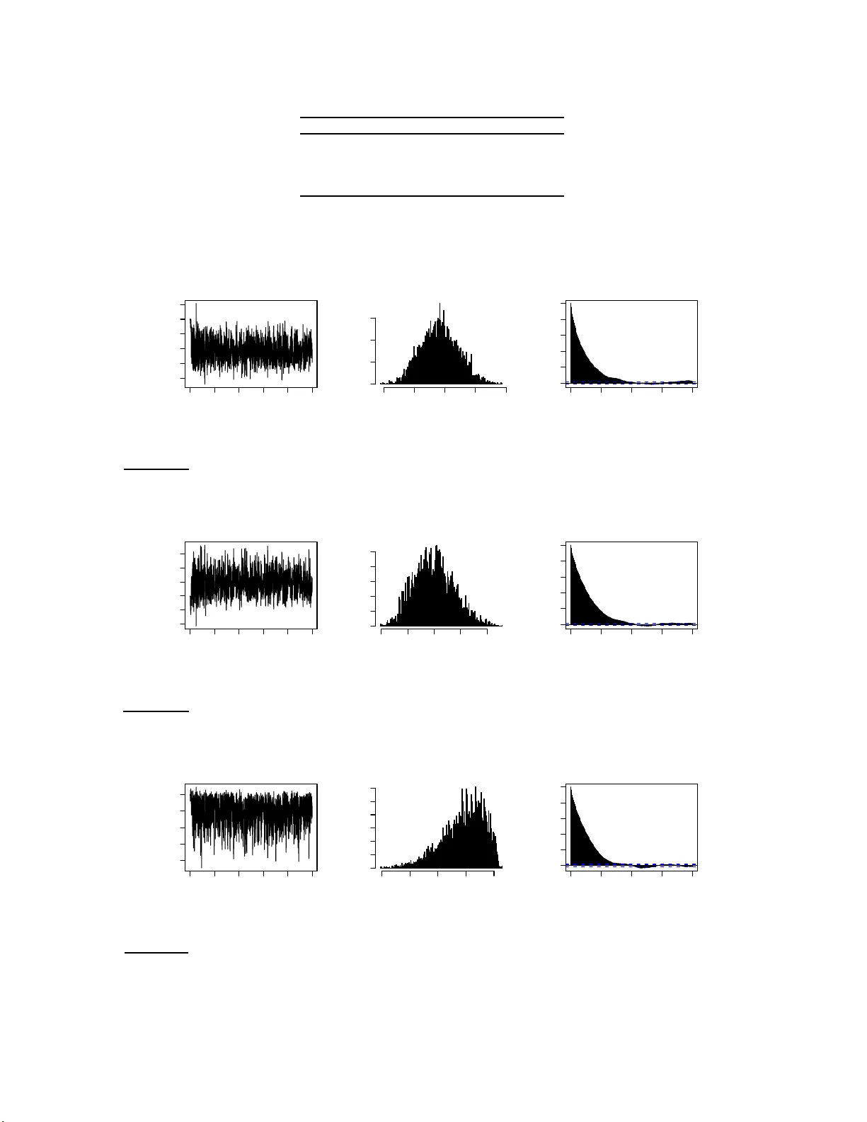
Ba y esian computation for statistic al mo de ls with in tractable normalizin g constan ts Yves F. A t chad´ e ∗ , Nic olas L artil lot † and Christian P. R ob ert ‡ (April 2008) Abstract: This pap er deals with some computational aspects in th e Bay esian analysis of statistica l mod els with intractable normali zing constan ts. In the presence of in tractable normalizing constants in th e lik eliho od function, traditional MCMC methods cannot b e applied. W e prop ose an approac h to sample from such p osterior distributions. The method can be thought as a Bay esian v ersion of the MCMC-MLE approac h of [8]. T o the b est o f our knowl edge, this is the first general and asympt otically consisten t Monte Carlo metho d for such problems. W e i llustrate the method with ex amp les f rom image seg mentation and social netw ork mo deling. W e stu dy as well the asymptotic b ehavior of th e algorithm and obtain a strong law of large numbers for empirical av erages. AMS 2000 sub ject cl assifications: Primary 60C05, 60J27, 60J3 5, 65C4 0. Keywords and phr ase s: Mo nte Carl o meth od s, A daptive MCMC, Ba yesia n inference, Ising mo del, Image segmen tation, So cial netw ork mo deling. 1. In tro duction Statistical inference for mod els with in tractable normalizing constan ts p oses a ma jor co mp uta- tional chall enge. This p roblem o ccurs in the statistical mod eling of man y scien tific p roblems. Examples includ e the analysis of spatial p oint pro cesses ([13]), image analysis ([10]), protein de- sign ([11]) and man y others. T he problem can b e describ ed as follo ws. Supp ose w e hav e a dataset x 0 ∈ ( X , B ) generated from a statistical mo d el e E ( x,θ ) λ ( dx ) / Z ( θ ) with parameter θ ∈ (Θ , Ξ), where t h e normaliz in g constan t Z ( θ ) = R X e E ( x,θ ) λ ( dx ) d ep ends on θ and is not a v ailable in closed form. Let µ b e the prior d en sit y of the p arameter θ ∈ (Θ , Ξ). The p osterior distribution of ∗ Department of Statistics, Universit y of Michiga n , email: yvesa @ u mic h .edu † LIRM, Un ivers it´ e d e Montpellier 2, email: nicolas.lartill ot@lirmm.fr ‡ CEREMADE, U n iversi t´ e Paris-Dauphine and CREST, INSEE, email: xian@ceremade.dauphine.fr 1 imsart ver. 2005/05/19 file: ALR08.tex date: November 10, 2018 /Bayesian c omputation for intr actable normalizing c onstants 2 θ giv en x 0 is then giv en b y π ( θ ) ∝ 1 Z ( θ ) e E ( x 0 ,θ ) µ ( θ ) . (1) When Z ( θ ) cannot b e easily ev aluated, Mon te Carlo sim u lation from this p osterior d istribution is problematic ev en using Mark o v Ch ain Monte Carlo (MCMC). [14] u ses the term doubly in- tr actable distr ibu tion to refer to posterior d istributions of the form (1). Cu rrent Mon te Carlo sampling metho ds do not allo w one to d eal with suc h m o dels in a Ba yesian framework. F or ex- ample, a Metrop olis-Hastings algorithm with prop osal kernel Q and target distribution π , wo u ld ha ve acce p tance ratio min  1 , e E ( x 0 ,θ ′ ) e E ( x 0 ,θ ) Z ( θ ) Z ( θ ′ ) Q ( θ ′ ,θ ) Q ( θ ,θ ′ )  whic h cannot b e compu ted as it in v olv es the in tractable n ormalizing constan t Z ev aluated at θ and θ ′ . An early atte mp t to deal with this prob lem is the pseu d o-lik eliho o d appro ximation of Besag ([4]) which approxima tes the mo d el e E ( x,θ ) b y a more tractable mo del. Pseudo-lik eliho o d in ference pro vides a fi rst appr oximati on but t ypically perf orms p o orly (see e.g. [5 ]). Maxim um lik eliho o d inference is p ossible. MCMC-MLE, a maxim u m lik eliho o d approac h us ing MCMC has b een d e- v elop ed in the 90’s ([7, 8]). Another related appr oac h to fi nd MLE estimates is Y ounes’ algo rith m ([18]) based on sto c hastic approximati on. An int eresting sim ulation study comparing these three metho ds is pr esented in [10]. Comparativ ely little wo r k has been done to d ev elop asymptotically exact metho ds for th e Ba y esian approac h to this problem. Bu t v arious appro ximate al gorithms exist in the lite r atur e, often based on path s ampling ([6]). Recen tly , [12] ha ve s ho wn that if exact sampling of X from e E ( x,θ ) / Z ( θ ) (as a density in ( X , B )) is p ossible then a v alid MCMC algorithm to sample from (1) can b e dev elop ed. See also [14] for some impro ve ments. T heir approac h uses a clev er auxiliary v ariable algo rith m . But intract able n ormalizing constan ts often occur in mo dels f or which exact sampling of X is not p ossib le or is very exp ensive. Another r ecent dev elopmen t to the problem is the app ro ximate Ba y esian computation sc hemes of Plagnol- T a v ar´ e ([ 15]) but whic h sample only appro ximately fr om the p osterior distrib ution. In this pap er, we pr op ose an adaptiv e Mon te Carlo approac h to sample from (1). Our algorithm generates a stochasti c p ro cess (not Mark o v in general) { ( X n , θ n ) , n ≥ 0 } in X × Θ suc h that as n → ∞ , the marginal distribution of θ n con v erges to (1 ). It is clear that any metho d to sample from (1 ) will ha v e to deal with the intracta ble normalizing constan t Z ( θ ). In the auxiliary v ariable metho d of [12], computing Z ( θ ) is replaced in a sense by p erfect sampling from e E ( x,θ ) / Z ( θ ). This imsart ver. 2005/05/19 file: ALR08.tex date: November 10, 2018 /Bayesian c omputation for intr actable normalizing c onstants 3 strategy w orks well so long as p erfect sampling is feasible and inexp ensive. In the present w ork, w e tak e another approac h b uilding on the idea of estimating the en tire function Z fr om a single Mon te Carlo sampler. The starting p oin t of the metho d is imp ortance sampling. Supp ose that for some θ (0) ∈ Θ, w e can sample (p erhaps b y MCMC) from the densit y e E ( x,θ (0) ) / Z ( θ (0) ) in ( X , B ). Using this sample, w e can certainly estimate Z ( θ ) / Z ( θ (0) ) for an y θ ∈ Θ. This is the same idea b ehind the MCMC-MLE algo rith m of [8]. But it is w ell kno wn that these estimates are t yp ically v ery p o or as θ gets far from θ (0) . No w, supp ose th at instead of a sin gle p oin t θ (0) , w e generate a p opulation { θ ( i ) , i = 1 , . . . , d } in Θ and that w e can sample from Λ ∗ ( x, i ) ∝ e E ( x,θ ( i ) ) / Z ( θ ( i ) ) on X × { 1 , . . . , d } . Th en w e sho w that in principle, efficie nt estimation for Z ( θ ) is p ossible for an y θ ∈ Θ. Building on [3] and the ideas sk etc hed ab o ve, we prop ose an algorithm that generates a random pro cess { ( X n , θ n ) , n ≥ 0 } suc h that the margi n al distribution of X n con v erges to Λ ∗ and the marginal distrib ution of θ n con v erges to (1). This random p ro cess is not a Mark o v chain in general but w e show (from firs t p rinciple) that { θ n } has limiting distribution π and satisfies a strong la w of large n umb ers. The pap er is organized as follo w s. A full description of the metho d including practical im- plemen tation details is giv en in Section 2. W e illustrate the alg orithm with th r ee examples. The Ising mo d el, a Ba yesia n image segmen tation example and a Ba ye sian m o deling of social net wo r k s . The examples are pr esen ted in Secti on 4. Some theoretical asp ects of the metho d are discussed in Section 3 with the pro ofs p ostp oned to 6. 2. Sampling from p osterior distributions with in tractable normalizing constan t s Throughout, w e fix the sample space ( X , B , λ ) and the parameter space (Θ , Ξ). Th e problem of in terest is to sample from the p osterior distribution (1) with Z ( θ ) = Z X e E ( x,θ ) λ ( dx ) . (2) Let { θ ( i ) , i = 1 , . . . , d } b e a sequence of d p oin ts in Θ. Let Λ ∗ b e the prob ab ility measure on X × { 1 , . . . , d } giv en b y: Λ ∗ ( x, i ) = e E ( x,θ ( i ) ) d Z ( θ ( i ) ) , x ∈ X , i ∈ { 1 , . . . , d } . (3) imsart ver. 2005/05/19 file: ALR08.tex date: November 10, 2018 /Bayesian c omputation for intr actable normalizing c onstants 4 Let κ ( θ , θ ′ ) b e a sim ilarity k ern el on Θ × Θ su c h that P d i =1 κ ( θ , θ ( i ) ) = 1 for all θ ∈ Θ. The starting p oint of th e algorithm is the follo win g decomp osition of th e p artition function: Z ( θ ) = Z X e E ( x,θ ) λ ( dx ) = d X i =1 κ ( θ , θ ( i ) ) Z X e E ( x,θ ) − E ( x,θ ( i ) ) e E ( x,θ ( i ) ) λ ( dx ) = d d X i =1 κ ( θ , θ ( i ) ) Z ( θ ( i ) ) Z X e E ( x,θ ) − E ( x,θ ( i ) ) e E ( x,θ ( i ) ) d Z ( θ ( i ) ) λ ( dx ) = d X i =1 Z X Λ ∗ ( x, i ) h θ ( x, i ) λ ( dx ) , (4) where h θ ( x, i ) = dκ ( θ , θ ( i ) ) Z ( θ ( i ) ) e E ( x,θ ) − E ( x,θ ( i ) ) . (5) The in terest of the decomp osition (4) is th at { Z ( θ ( i ) ) } and Λ ∗ do not d ep end on θ . T herefore, using samples from Λ ∗ , this decomp osition giv es an approac h to estimate Z ( θ ) for all θ ∈ Θ. This estimate sh ould b e reliable p ro vided θ is close to at least one particle θ ( i ) . The p roblem of sampling from p robabilit y measures suc h as Λ ∗ has b een rece ntly considered b y [3] building on the W ang-Landau algorithm of [17]. W e follo w and impro v e that approac h here. The resulting estimate of Z ( θ ) can then cont inuously b e fed to a second Mon te Carlo sampler that carries the sim ulation with resp ect to π . T his su ggests an adaptiv e Mon te Carlo sampler to sample from (1) whic h we dev elop next. F or any c = ( c (1) , . . . , c ( d )) ∈ R d , we d efine the follo wing densit y fu nction on X × { 1 , . . . , d } : Λ c ( x, i ) ∝ e E ( x,θ ( i ) ) − c ( i ) . (6) With c = log ( Z ), Λ c = Λ ∗ . The reader should thin k of c as an estimate of z , with z ( i ) := log Z ( θ ( i ) ). The algorithm will adaptiv ely adjus t c suc h that th e marginal distr ib ution on { 1 , . . . , d } is appro ximately uniform. In which case, w e should hav e c ( i ) = log Z ( i ). Let { γ n } b e a sequ ence of (p ossibly random) p ositiv e n umb ers. W e prop ose a non-Marko vian adaptiv e sampler that lives in X × { 1 , . . . , d } × R d × Θ. W e start from an initial state ( X 0 , I 0 , c 0 , θ 0 ) ∈ X × { 1 , . . . , d } × R d × Θ, where c 0 ∈ R d is the initial estimate of z . F or example, c 0 ≡ 0. At time n , giv en ( X n , I n , c n , θ n ) we first generate X n +1 from P I n ( X n , · ), where P i is a transition k ern el on ( X , B ) w ith in v ariant d istri- bution e E ( x,θ ( i ) ) / Z ( θ ( i ) ). Next, w e generate I n +1 from the distribution on { 1 , . . . , d } prop ortional imsart ver. 2005/05/19 file: ALR08.tex date: November 10, 2018 /Bayesian c omputation for intr actable normalizing c onstants 5 to e E ( X n +1 ,θ ( i ) ) − c n ( i ) . Then we u p d ate the current estimate of log( Z ) to c n +1 giv en by: c n +1 ( i ) = c n ( i ) + γ n e E ( X n +1 ,θ ( i ) ) − c n ( i ) P d j =1 e E ( X n +1 ,θ ( j ) ) − c n ( j ) , i = 1 , . . . , d. (7) In view of (4), we can estimate Z ( θ ) by: Z n +1 ( θ ) = d X i =1 κ ( θ , θ ( i ) ) e c n +1 ( i ) " P n +1 k =1 e E ( X k ,θ ) − E ( X k ,θ ( i ) ) 1 i ( I k ) P n +1 k =1 1 i ( I k ) # , (8) with the conv ention that 0 / 0 = 0. Finally , for an y p ositiv e function ζ : Θ → (0 , ∞ ), let Q ζ b e a transition ke rn el on (Θ , Ξ) w ith in v arian t distribution π ζ ( θ ) ∝ 1 ζ ( θ ) e E ( x 0 ,θ ) µ ( θ ) . (9) Giv en ( X n +1 , I n +1 , c n +1 , Z n +1 , θ n ), we generate θ n +1 from Q Z n +1 ( θ n , · ), where Z n +1 is the fun ction defined by (8). The algorithm can b e summarized as follo ws. Algorithm 2.1. . L et ( X 0 , I 0 , c 0 , θ 0 ) ∈ X × { 1 , . . . , d } × R d × Θ b e the initial state of the algorithm. L et { γ n } b e (a p ossibly r andom) se quenc e of p ositive numb e rs. At time n , given ( X n , I n , c n , θ n ) : 1. Gener ate X n +1 fr om P I n ( X n , · ) wher e P i is any er go dic kernel on ( X , B ) with invaria nt dis- tribution e E ( x,θ ( i ) ) / Z ( i ) . 2. Gener ate I n +1 by sampling fr om the distribution on { 1 , . . . , d } pr op ortional to e E ( X n +1 ,θ ( i ) ) − c n ( i ) . 3. Compute c n +1 , the new estimate of g using (7). 4. Using the fu nction Z n +1 define d by (8), g ener ate θ n +1 fr om Q Z n +1 ( θ n , · ) . Remark 2.1 . 1. The algorithm can b e seen as an MCMC-MCMC analog to the MCMC-MLE of [8]. Indeed, with d = 1, the decomp osition (4) b ecomes Z ( θ ) / Z ( θ (1) ) = E h e E ( θ,X ) − E ( X, θ (1) ) i , where the exp ectation is tak en with resp ect to the d ensit y e E ( x,θ (1) ) / Z ( θ (1) ). But as discussed in the in tro d uction, when E ( θ , X ) − E ( X , θ (1) ) has a large v ariance, the resulting estimate is terribly p o or. 2. W e int r o duce κ to serve as a smo othing f actor so that the particles θ ( i ) ’s close to θ contribute more to the estimation of Z ( θ ). W e exp ect this smo othing step to reduce the v ariance of imsart ver. 2005/05/19 file: ALR08.tex date: November 10, 2018 /Bayesian c omputation for intr actable normalizing c onstants 6 the o v erall estimate of Z ( θ ). In th e simula tions w e c h o ose κ ( θ , θ ( i ) ) = e − 1 2 h 2 k θ − θ ( i ) k 2 P d j =1 e − 1 2 h 2 k θ − θ ( j ) k 2 . The v alue of the smo othing parameter h is set by trials and errors for eac h example. 3. The implemen tation of the algorithm requires k eeping trac k of all the samples X k that are generated (Equation (8 )). X can b e a v ery high-dimensional space and we are a w are of the fact that in practice , this b o okk eeping can significant ly slo w do wn the algorithm. But in man y cases, the f unction E tak es the form E ( x, θ ) = P K l =1 S l ( x ) θ l for some real-v alued func- tions S l . In these cases, we only n eed to kee p track of the statistics { ( S 1 ( X n ) , . . . , S K ( X n )) , n ≥ 0 } . All the examples d iscussed in the pap er f all in this latter category . 4. As men tioned earlier, the up date of ( X n , I n , c n ) is essen tially the W ang-Landau algorithm of [3] w ith the follo wing imp ortan t difference. [3] p rop ose to up date c n one comp onent p er iteration: c n +1 ( i ) = c n ( i ) + γ n 1 { i } ( I n +1 ) . W e imp r o v e on this sc heme in (7) b y Rao-Blac k welliza tion where w e in tegrate out I n +1 . 5. As menti oned ab o v e, and we stress th is again, this algorithm is not Marko vian in an y wa y . The pro cess { ( X n , I n , c n ) } is not a Mark ov chain but a nonhomogeneous Marko v c hain if w e let { γ n } b e a deterministic sequence. { θ n } , the main random pr o cess of in terest is not a Mark o v c hain either. Nev er th eless, the marginal distribution of θ n will t ypically con v erge to π . This is b ecause, Q Z n , the conditional distribu tion of θ n +1 giv en F n con v erges to Q Z as n → ∞ and Q Z is a kernel with in v arian t distribution π . W e make this precise by sho wing that a strong la w of large n umb ers holds for additiv e functionals of { θ n } . W e no w discuss the c h oice of the parameters of the algo rith m . 2.1. Cho osing d a nd the p ar ticles { θ ( i ) } W e do not h a v e an y general approac h in c h o osing d and { θ ( i ) } but we giv e some guidelines. Th e general idea is that the particles { θ ( i ) } need to co v er r easonably w ell the r ange of the density π and b e suc h that for an y θ ∈ Θ, the density e E ( x,θ ) / Z ( θ ) in X can b e w ell appro ximated by at least one of the densities e E ( x,θ ( i ) ) / Z ( i ). On e p ossibilit y is to sample θ ( i ) indep end en tly from the imsart ver. 2005/05/19 file: ALR08.tex date: November 10, 2018 /Bayesian c omputation for intr actable normalizing c onstants 7 prior distribution µ , some temp ered v ersion of it o r some other similar d istribution. W e follo w this app roac h in the examples b elo w. Another p ossibilit y is to use a grid of p oin ts in Θ. The v alue of d , the n um b er of particle s, should dep end on the size of Θ. W e need to c ho ose d suc h that the distributions e E ( x,θ ( i ) ) / Z ( i ) (in X ) o ve r lap. Otherwise, estimating the constan ts { Z ( i ) } can b e d iffi cu lt. This implies that d should not b e to o small. I n the simulatio n examples b e! lo w w e choose d b et we en 100 and 500. 2.2. Cho osing the step-size { γ n } It is shown in [3] that the recur s ion (7) can also b e wr itten as a sto c hastic ap p ro ximation algorithm with step-size { γ n } , so that i n theory , an y p ositiv e sequence { γ n } s uc h that P γ n = ∞ and P γ 2 n < ∞ can b e used. But the con v ergence of c n to log Z is v ery sensitiv e to the c hoice { γ n } . If the γ n ’s are o v erly s mall, the recursiv e equation in (7) will mak e v ery small steps. But if these n umb ers are o verly large, the algorithm will h a v e a large v ariance. In b oth cases, the con verge n ce to the solution w ill b e slow. Overall, choosing the righ t step-size for a stochastic app r o ximation algorithm is a difficult problem. Here we follo w [3] whic h has elab orated on a heu r istic approac h to this pr oblem originall y prop osed by [17]. The main idea of the metho d is that typical ly , the larger γ n , the easier it is for the algorithm to mo ve aroun d the state space. Therefore, at the b eginning γ 0 is s et at a relativ ely large v alue. This v alue is k ept until { I n } h as visited equally w ell all th e points of { 1 , . . . , d } . Let τ 1 b e the first time where the occup ation measure of { 1 , . . . , d } by { I n } is app ro ximately un iform. Then w e set γ τ 1 +1 to some smaller v alue (for example γ τ 1 +1 = γ τ 1 / 2) and th e pr o cess is iterated unt il γ n b ecome sufficien tly small. As wh ich p oin t w e can c h o ose to switc h to a deterministic sequence of the form γ n = n − 1 / 2 − ε . Combining th is id ea with Algorithm 2.1, we get the follo wing. Algorithm 2.2. . L et γ > ε 1 > 0 , ε 2 > 0 b e c onstants a nd let ( X 0 , I 0 , c 0 , θ 0 ) b e some a rbitr ary initial state of the algorithm. Set v = 0 ∈ R d and n = 0 . While γ > ε 1 and given F n = σ { ( X k , I k , c k , θ k ) , k ≤ n } , 1. Gener ate ( X n +1 , I n +1 , c n +1 , θ n +1 ) as in Algorithm 2.1. 2. F or i = 1 , . . . , d : set v ( i ) = v ( i ) + 1 i ( I n +1 ) . 3. If max i    v ( i ) − 1 d    ≤ ε 2 d , then se t γ = γ / 2 and set v = 0 ∈ R d . imsart ver. 2005/05/19 file: ALR08.tex date: November 10, 2018 /Bayesian c omputation for intr actable normalizing c onstants 8 Remark 2.2. W e use this algorithm in the examples b elo w with the follo w in g sp ecifications. W e set the initial γ to 1, ε 2 = 0 . 2. W e run { ( X n , I n , c n ) } un til γ ≤ ε 1 = 0 . 001 b efore starting { θ n } and switc hing to a deterministic sequence γ n = ε 1 /n 0 . 7 . 3. Conv ergence analysis In this s ection, w e deriv e a la w of large n umbers u nder some verifiable conditions. The pro cess of interest her e is { θ n } . Let (Ω , F , Pr ) b e the reference probabilit y triplet. W e equ ip (Ω , F , Pr ) with the filtration {F n } , where F n = σ { ( X k +1 , I k +1 , c k +1 , θ k ) , k ≤ n } . Note that F n includes ( X n +1 , I n +1 , c n +1 ) since these rand om v ariables are used in generat in g θ n +1 . F rom th e definition of the algorithm, we h a v e: Pr ( θ n +1 ∈ A |F n ) = Q Z n +1 ( θ n , A ) , Pr − a.s.. (10) W e see from (10) that { θ n , F n } is an adaptiv e Mon te C arlo algo r ithm with v aryin g target distri- bution. In analyzing { θ n , F n } h ere, we do not striv e for the most general r esu lt but r estrict ourself to conditions that can b e easily c h ec k ed in the examples considered in the pap er. W e assume that Θ is a compact subset of R q , the q -dimensional Euclidean space equipp ed with its Borel σ -algebra and the Leb esgue measure. Firs tly , we assume that the fun ction E is b ounded: (A1) : Ther e exist m, M ∈ R such that: m ≤ E ( x, θ ) ≤ M , x ∈ X , θ ∈ Θ . (11) In man y a p plications, and this is th e c ase for th e examples discussed b elo w, X is a fin ite set (t ypically v ery large) and Θ is a compact set. In th ese cases, (A1) is easily c hec ked. In ord er to pro ceed any fur ther, we n eed some notations. A transition kernel on ( X , B ) op erates on measurable real-v alued functions f as P f ( x ) = R P ( x, dy ) f ( y ), and the pro du ct of t wo transition k ernels P 1 and P 2 is the transition kernel defined as P 1 P 2 ( x, A ) = R P 1 ( x, dy ) P 2 ( y , A ). W e can then defin e recursiv ely P n = P P n − 1 , n ≥ 1, P 0 ( x, A ) = 1 A ( x ). F or t wo p robabilit y measures µ, ν , the total v ariation distance b et we en µ and ν is defin ed as k µ − ν k T V := sup A | µ ( A ) − ν ( A ) | . W e sa y that a transition kernel P is geometricall y ergo d ic if P is φ -irredu cible, ap erio dic and has an inv arian t distribution π such th at: k P n ( x, · ) − π k T V ≤ M ( x ) ρ n , n ≥ 0 imsart ver. 2005/05/19 file: ALR08.tex date: November 10, 2018 /Bayesian c omputation for intr actable normalizing c onstants 9 for some ρ ∈ (0 , 1) and some function M : X → (0 , ∞ ]. Our next assump tion inv olv es the transition ke rn el Q ζ . (A2) : F or ζ : Θ → (0 , ∞ ) , Q ζ is a Metr op olis kernel with i nvariant distribution π ζ and pr op osal kernel density p . Ther e e xist ε > 0 and an inte ger n 0 ≥ 1 such that for al l θ , θ ′ ∈ Θ : p n 0 ( θ , θ ′ ) ≥ ε. (12) Remark 3.1 . 1. The cond ition (12) clearly h olds for most symmetric p r op osal k ern els p ( θ , θ ′ ), pro vided th at p ( θ , θ ′ ) remains b ounded a wa y f r om 0 on some ball cen tered at θ . 2. (12) often imp lies that Q ζ is uniformly ergo dic: Q ζ ( θ , A ) ≥ Z A min  1 , e E ( x 0 ,θ ′ ) − E ( x 0 ,θ ) ζ ( θ ′ ) ζ ( θ )  p ( θ , θ ′ ) dθ ′ ≥ e m − M inf θ , θ ′ ∈ Θ  ζ ( θ ) ζ ( θ ′ )  Z A p ( θ , θ ′ ) dθ ′ . Therefore, pro vided inf θ , θ ′ ∈ Θ  ζ ( θ ) ζ ( θ ′ )  > 0, if (12) hold then Q n 0 ζ ( θ , A ) ≥ ε ′ µ Leb ( A ) for s ome ε ′ > 0. (A3) : { γ n } is a r andom se quenc e, adapte d to {F n } such that γ n > 0 , P γ n = ∞ and P γ 2 n < ∞ Pr -a.s. Theorem 3.1. Assume (A1)-(A 3). Assume also tha t e ach ke rnel P i on ( X , B ) i s ge ometric al ly er go dic. L et h : (Θ , Σ) → R such that | h | ≤ 1 . Then: 1 n n X k =1 h ( θ k ) → π ( h ) , Pr − a.s. (13) Pr o of. See Section 6. 4. Examples 4.1. Ising mo del W e test th e algorithm with the Ising mo d el on a rectangular lattice . Th is is a s im ulated example. The mo del is given b y e θ E ( x ) / Z ( θ ) wh er e E ( x ) = m X i =1 n − 1 X j =1 x ij x i,j +1 + m − 1 X i =1 n X j =1 x ij x i +1 ,j , (14) imsart ver. 2005/05/19 file: ALR08.tex date: November 10, 2018 /Bayesian c omputation for intr actable normalizing c onstants 10 and x i ∈ { 1 , − 1 } . W e u se m = n = 64. W e generate the d ata x 0 from e θ E ( x ) / Z ( θ ) with θ = 0 . 40 b y p erfect sampling using the Propp -Wilson alg orithm. Using x 0 and p ostulating th e mo del e θ E ( x ) / Z ( θ ), w e would lik e t o infer on θ . W e use the prior µ ( θ ) = 1 (0 , 1) ( θ ). W e set d = 100 and generate the p oin ts { θ ( i ) } indep endentl y and uniformly in (0 , 1). As d escrib ed in Section 2.2, we use the flat histogram approac h in selecting { γ n } with an initial v alue γ 0 = 1, u n til γ n b ecomes sm aller than 0 . 001. Then we start feeding the adaptive c hain { θ n } which is run for 10 , 000 iterations. In up d ating θ n , w e use a Random W alk Metropolis sampler with prop osal distribution U ( θ n − b, θ n + b ) (with reflexion at the b oun daries) for some b > 0. W e adaptiv ely up date b so as to reac h an acce p tance rate of 30% (see e.g. [2]). W e d! iscard th! e first 1 , 999 p oin ts as a b urn-in p erio d. The results are p lotted on Figure 1. As w e can see from these plots, the samp ler ap p ears to ha ve con verged to th e p osterior distr ib ution π . The mixing rate of the algorithm a s inferred from the auto correlation function seems fairly go o d. In addition, the algo rith m yields an estimate of the partition fu n ction log Z ( θ ) which can b e re-used in other sampling problems. 0.0 0.2 0.4 0.6 0.8 1.0 17000 19000 21000 (a) 0 2000 4000 6000 8000 0.38 0.39 0.40 0.41 0.42 (b) 0.38 0.39 0.40 0.41 0.42 0 50 100 200 300 (c) 0 100 200 300 400 0.0 0.2 0.4 0.6 0.8 1.0 (d) Figure 1: Outp u t for the Ising mo del θ = 0 . 40, m = n = 64. (a): estimation of log Z ( θ ) up to an additiv e constan t; (b)-(d): T race plot, histogram and autocorrelation fu nction of the adaptiv e sampler { θ n } . imsart ver. 2005/05/19 file: ALR08.tex date: November 10, 2018 /Bayesian c omputation for intr actable normalizing c onstants 11 4.2. An applic ation to image se gmentation W e use the Isin g mo del ab o v e to illustrate an application of the metho dology to image segmen- tation. In image segmenta tion, the goal is the r econstruction of images f rom noisy observ ations (see e.g. [9 , 10]). W e repr esen t the image b y a v ector x = { x i , i ∈ S } where S is a m × n lattice and x i ∈ { 1 , . . . , K } . Eac h i ∈ S represents a pixel, and x i is the color of the pixel i . K i s the n umb er of colors. Here w e assume that K = 2 and x i ∈ {− 1 , 1 } is either blac k or white. In the image segmen tation problem, we do not observ e x but a noisy app ro ximation y . W e assume that: y i | x, σ 2 ind ∼ N ( x i , σ 2 ) , (15) for some unknown parameter σ 2 . Even though (15) is a cont inuous mo d el, it has b een shown to pro vide a relati vely goo d framew ork for imag e s egmentat ion problems w ith m ultiple additiv e sources of noise ([10 ]). W e assu me that the t r ue image x is g enerated from an Ising mo d el (see Section 4.1) w ith in teraction parameter θ . W e assume t h at θ follo w s a uniform prior distrib u tion on (0 , 1) and that σ 2 has a p rior distribution that is p rop ortional to 1 /σ 2 1 (0 , ∞ ) ( σ 2 ). The p osterior distribution ( θ , σ 2 , x ) is then giv en b y: π  θ , σ 2 , x | y  ∝  1 σ 2  |S | 2 +1 e θ E ( x ) Z ( θ ) e − 1 2 σ 2 P s ∈S ( y ( s ) − x ( s )) 2 1 (0 , 1) ( θ ) 1 (0 , ∞ ) ( σ 2 ) , (16) where E is as in (14). W e sample from this p osterior distribution using th e adaptiv e c hain { ( y n , i n , c n , θ n , σ 2 n , x n ) } . The c hain { ( y n , i n , c n ) } is up dated follo wing Steps (1)-(3) of Algorithm 2.1. It is used to form the ad ap tive estimate of Z ( θ ) as giv en by (8) (with { y n , i n } r ep lacing { X n , I n } ). Th ese estimates are u s ed to up date ( θ n , σ 2 n , x n ) u sing a Metropolis-within-Gibbs sc heme. More sp ecifically , giv en σ 2 n , x n , we sample θ n +1 with a Random W alk Metrop olis with prop osal U ( θ n − b, θ n + b ) (with reflexion at the b oundaries) and target prop ortional to e θE ( x n ) Z n ( θ ) . Given θ n +1 , x n , we generate σ 2 n +1 b y s ampling from the In verse-Ga mm a distribu tion with parameters ( |S | 2 , 1 2 P s ∈S ( y ( s ) − x ( s )) 2 ). And giv en ( θ n +1 , σ n +1 ), we sample eac h x n +1 ( s ) from its conditional distribu tion giv en { x ( u ) , u 6 = s } . This conditional d istribution is giv en b y p ( x ( s ) = a | x ( u ) , u 6 = s ) ∝ exp θ a X u ∼ s x ( u ) − 1 2 σ 2 ( y ( s ) − a ) 2 ! , a ∈ {− 1 , 1 } . imsart ver. 2005/05/19 file: ALR08.tex date: November 10, 2018 /Bayesian c omputation for intr actable normalizing c onstants 12 Here u ∼ v means that pixels u and v are neigh b ors. T o test this algo rith m , w e generate a simulate d dataset y according to mo del (15) with x generated from e θ E ( x ) / Z ( θ ) b y p erfect sampling. W e us e m = n = 64, θ = 0 . 40 and σ = 0 . 5. F or the implemen tation details of the algorithm, we mak e exactly th e same c hoices as in Example 4.1 abov e. In particular we c ho ose d = 100 and generate { θ ( i ) } u niformly in (0 , 1). Th e results are giv en in Figure 2. Once again, the sample path obtained from { θ n } clearly su ggests that the distribution of θ n has conv erged to π with a goo d m ixin g r ate, as inferr ed from the auto correlation plots. 0 2000 4000 6000 8000 0.38 0.39 0.40 0.41 (a) 0.38 0.39 0.40 0.41 0 50 100 150 200 250 300 (b) 0 100 200 300 400 0.0 0.2 0.4 0.6 0.8 1.0 (c) 0 2000 4000 6000 8000 0.24 0.25 0.26 0.27 0.28 (d) 0.24 0.25 0.26 0.27 0.28 0 50 100 150 200 250 300 (e) 0 100 200 300 400 0.0 0.2 0.4 0.6 0.8 1.0 (f) Figure 2: Output for the image segmenta tion mod el. (a)-(c): plots of { θ n } ; (d)-(f ): plots of { σ n } . 4.3. So cial networ k mo d eling W e now giv e an app lication of the metho d to a Ba yesia n analysis of social netw orks. Stati stical mo deling of so cial net work is a gro wing su b ject in so cial science (See e.g. [16] and the r eferences therein for more details). Th e set up is the follo wing. W e ha v e n actors I = { 1 , . . . , n } . F or eac h pair ( i, j ) ∈ I × I , define y ij = 1 if actor i has ties with actor j and y ij = 0 otherwise. In the example b elo w, we only consider the case of a symmetric relationship where y ij = y j i for all i, j . The ties referr ed to here can b e of v arious natures. F or exa m p le, w e might b e interested in imsart ver. 2005/05/19 file: ALR08.tex date: November 10, 2018 /Bayesian c omputation for intr actable normalizing c onstants 13 mo deling ho w fr iendships build up b et we en co-w orkers or ho w researc h col lab oration tak es place b et ween collea gues. Another inte r esting example from p olitical science is mod eling co-sp onsorship ties (for a giv en p iece of legislation) b etw een mem b ers of a hous e of representa tives or parlimen t. In th is example we study the Medici business net w ork dataset tak en from [16] whic h describ es the business ties b et ween 16 Floren tine families. Num b ering arbitrarily the family from 1 to 16, w e plot the observed so cial net w ork in Figure 3. Th e dataset conta ins relat ively few ties b et ween families and ev en few er transitive ties. 1 9 2 6 7 3 5 4 11 15 8 16 13 14 10 12 Figure 3: Business Relationships b et we en 16 Floren tine families. One of the most p opular m o dels for so cial net wo r ks is the class of exp onen tial random graph mo dels. In these m o dels, w e assu m e that { y ij } is a sample generated f rom the distribution p ( y | θ 1 , . . . , θ K ) ∝ exp K X i =1 θ i S i ( y ) ! , (17) for some parameters θ 1 , . . . , θ K ; where S i ( y ) is a statistic used to capture some asp ect of the net wo r k. F or this example, and follo win g [16], we consider a 4-dimensional mo d el with statistics S 1 ( y ) = X i 0 and a p ositiv e definite matrix Σ. W e adaptiv ely set σ so as to reac h an acceptance rate of 30%. Ideally , we w ould lik e to c ho ose Σ = Σ π the v ariance-co v ariance of π whic h of course, is not av ailable. W e adaptive ly estimate Σ π during the sim ulation as in [2]. As b efore, we run ( X n , I n , c n ) un til γ n < 0 . !001 . Then w e sta r t { θ n } and run the full c h ain ( X n , I n , c n , θ n ) for a total of 25 , 000 iterat ions. The p osterior distri- butions of the parameters are giv en in Figur es 4a-4d. In T able 1, w e giv e the sample p osterior mean together with the 2 . 5% and 97 . 5% quan tiles of the p osterior distribution. Overall, these r e- sults are consisten t with the maxim um likelihoo d estimates obtained by [16] usin g MCMC-MLE. The main difference app ears in θ 4 whic h we fi nd here not to b e significant. As a b y-pro d uct, the sampler giv es an estimate of the v ariance-co v ariance matrix of th e p osterior distrib ution π : Σ π =          1.67 -0.41 0.27 -0.07 -0.41 1.83 -0.47 - 0.02 0.27 -0.47 1.78 -0.03 -0.07 - 0.02 -0.03 1.65          . (19) imsart ver. 2005/05/19 file: ALR08.tex date: November 10, 2018 /Bayesian c omputation for intr actable normalizing c onstants 15 P arameters P ost. mean P ost. quantiles θ 1 − 2 . 14 ( − 3 . 32 , − 0 . 81) θ 2 0 . 94 ( − 0 . 43 , 2 . 49) θ 3 − 1 . 06 ( − 2 . 72 , 0 . 04) θ 4 0 . 09 ( − 1 . 39 , 1 . 07) T able 1 Summary of the p osterior distribution of the p ar ameters. Posterior me ans, 2 . 5% and 97 . 5% quantiles 0 5000 15000 25000 −4 −2 0 1 (a) (b) −4 −3 −2 −1 0 0 100 200 300 0 50 100 150 200 0.0 0.4 0.8 (c) Figure 4a: Th e adap tive MCMC output from (18 ). (a)-(c ): Plots f or { θ 1 } . Based on 25 , 000 iterations. 0 5000 15000 25000 −2 0 1 2 3 (a) (b) −1 0 1 2 3 0 50 150 250 0 50 100 150 200 0.0 0.4 0.8 (c) Figure 4b: The adaptiv e MCMC output from (18). (a)-(c): P lots for { θ 2 } . Based on 25 , 000 iterations. 0 5000 15000 25000 −4 −3 −2 −1 0 (a) (b) −4 −3 −2 −1 0 0 50 150 250 0 50 100 150 200 0.0 0.4 0.8 (c) Figure 4c: The adaptiv e MCMC output from (18). (a)-(c): P lots for { θ 3 } . Based on 25 , 000 iterations. imsart ver. 2005/05/19 file: ALR08.tex date: November 10, 2018 /Bayesian c omputation for intr actable normalizing c onstants 16 0 5000 15000 25000 −3 −2 −1 0 1 (a) (b) −3 −2 −1 0 1 0 100 200 300 400 0 50 100 150 200 0.0 0.4 0.8 (c) Figure 4d: The adaptiv e MCMC output from (18). (a)-(c): P lots for { θ 4 } . Based on 25 , 000 iterations. 5. Conclusion Sampling fr om p osterior distributions with intracta ble n ormalizing constan ts is a d iffi cu lt compu- tational pr oblem. T h u s far, all metho ds prop osed in the literature but one en tail approximat ions that do not v anish asymptotically . And the only exception ([12]) requir es exact sampling in the data space, which is on ly possib le for v ery sp ecific cases. In this work, w e prop ose an approac h that b oth is more general than [12] and satisfies a s trong la w of large n umb ers w ith limiting distribution equal to the target distribu tion. The few applications w e ha ve p resen ted here su g- gest th at the metho d is promising. It remains to b e determined ho w the metho d will scale with the dimensionalit y and with the size of th e problems, although in this resp ect, adaptations of the metho d in v olving annealing/temperin g schemes are easy to imagine, whic h would allo w large problems to b e analysed p rop erly . Ac kno wledgements The researc h of the third author had b een partly su pp orted b y the Agence Nationale de la Rec herc h e (ANR, 212, rue de Bercy 75012 Paris) through the 2006-200 8 p r o ject Adap’MC . 6. Pro of of Theorem 3.1 Pr o of. Th r ough tout th e pro of, C will d enote a finite constan t but wh ose actual v alue can c hange from one equation to the next. T he conv ergence of the W ang-Landau algorithm has b een studied in [3]. It is sho wn in th is w ork that under the cond ition of Theorem 3.1, min i P ∞ k =1 1 { i } ( I k ) = ∞ and imsart ver. 2005/05/19 file: ALR08.tex date: November 10, 2018 /Bayesian c omputation for intr actable normalizing c onstants 17 more imp ortan tly , e c n ( i ) / P d j =1 e c n ( j ) con v erges almost su rely to a Z ( θ ( i ) ) (up to a m ultiplicativ e constan t). Define ω n ( i ) = e c n ( i ) P d j =1 e c n ( j ) , v n,i ( θ ) = P n k =1 e E ( X k ,θ ) − E ( X k ,θ ( i ) ) 1 i ( I k ) P n k =1 1 i ( I k ) and ˜ Z n ( θ ) := Z n ( θ ) P d j =1 e c n ( j ) = d X i =1 ω n ( i ) v n,i ( θ ) . (20) Instead of Z n , w e work with ˜ Z n . This is equiv alen t b ecause P d j =1 e c n ( j ) do es not d ep end on θ and Z n alw a ys app ears in Q Z n as a ratio. W e ha v e: inf θ ∈ Θ ˜ Z n ( θ ) ≥ e m − M . (21) inf θ , θ ′ ∈ Θ ˜ Z n ( θ ) ˜ Z n ( θ ′ ) ! ≥ e 2( m − M ) . (22) Com binin g (22) and (12) and part 2 of R emark 3.1, we dedu ce that there exists ε 0 > 0 suc h that for all n, j ≥ 0 sup | h |≤ 1    Q j Z n h ( θ ) − π Z n ( h )    ≤ 2(1 − ε 0 ) j , Pr − a.s. (23) W e in tro du ce the n otation ¯ Q n = Q ˜ Z n − π ˜ Z n . It f ollo w s from (23) that for an y n ≥ 1 the follo win g function g n is w ell defined: g n ( θ ) = ∞ X j =1 ¯ Q j n h ( θ ) . Moreo v er | g n ( θ ) | ≤ 2 /ε 0 for all θ ∈ Θ. g n satisfies Po isson’s equation for ¯ Q n and h − π ˜ Z n ( h ): g n ( θ ) − ¯ Q n g n ( θ ) = h − π Z n ( h ) . (24) Using this we can rewrite P n k =1 h ( θ k ) − π Z k ( h ) as: 1 n n X k =1 ( h ( θ k ) − π Z k ( h )) = 1 n n X k =1  g k ( θ k ) − ¯ Q k g k ( θ k − 1 )  + 1 n n X k =1  ¯ Q k g k ( θ k − 1 ) − ¯ Q k − 1 g k − 1 ( θ k − 1 )  + 1 n  ¯ Q 0 g 0 ( θ 0 ) − ¯ Q n g n ( θ n )  . (25) imsart ver. 2005/05/19 file: ALR08.tex date: November 10, 2018 /Bayesian c omputation for intr actable normalizing c onstants 18 Since su p θ ∈ Θ | g n ( θ ) | ≤ 2 /ε 0 , a similar b ound h old for ¯ Q n g n and we conclud e that 1 n  ¯ Q 0 g 0 ( θ 0 ) − ¯ Q n g n ( θ n )  actually co nv erges almost surely to 0 as n → ∞ . W riting D k = g k ( θ k ) − ¯ Q k g k ( θ k − 1 ), it is eas- ily seen that { D k , F k } is a martin gale difference with b ounded in cr ement and w e deduce from martingales theory that 1 n P n k =1  g k ( θ k ) − ¯ Q k g k ( θ k − 1 )  con v erges almost surely to 0 as n → ∞ . Since Q Z is a Metrop olis k ernel and u sing the fact th at | min(1 , ax ) − min(1 , ay ) | ≤ a | x − y | for all a, x, y ≥ 0 we d educe that for any f unction h : Θ → R suc h that | h | ≤ 1,    ( Q ˜ Z n − Q ˜ Z n − 1 ) h ( θ )    ≤ Z      ˜ Z n ( θ ) ˜ Z n ( θ ′ ) − ˜ Z n − 1 ( θ ) ˜ Z n − 1 ( θ ′ )      e E ( x 0 ,θ ′ ) − E ( x 0 ,θ ) p ( θ , θ ′ )   h ( θ ′ ) − h ( θ )   dθ ′ ≤ 2 e M − m sup θ , θ ′ ∈ Θ      ˜ Z n ( θ ) ˜ Z n ( θ ′ ) − ˜ Z n − 1 ( θ ) ˜ Z n − 1 ( θ ′ )      ≤ C    ˜ Z n ( θ ) − ˜ Z n − 1 ( θ )    , using (21 − 22) , (26) for some finite constan t. Combining (23 and 26) w e ha ve the follo w ing w ell-kno wn consequence: there exists C < ∞ such that for all n ≥ 1: sup | h |≤ 1    π ˜ Z n ( h ) − π ˜ Z n − 1 ( h )    ≤ C sup θ ∈ Θ    ˜ Z n ( θ ) − ˜ Z n − 1 ( θ )    . (27) The stabilit y of P oisson’s equation for geometrically ergod ic tran s ition kernels is w ell kno wn (see e.g. [1, 3]). Combining (23), (26) and (27), we can find a finite constan t C suc h that for all k ≥ 1:    ¯ Q k g k ( θ k − 1 ) − ¯ Q k − 1 g k − 1 ( θ k − 1 )    ≤ C sup θ , θ ′ ∈ Θ    ˜ Z k ( θ ) − ˜ Z k − 1 ( θ )    . (28) Giv en the expression of ˜ Z n ( θ ) in (20) it is not v ery hard to sho w there exists C < ∞ suc h that: sup θ ∈ Θ    ˜ Z k ( θ ) − ˜ Z k − 1 ( θ )    ≤ C dγ k + 1 min i P k l =1 1 { i } ( I l ) ! → 0 , (29) as k → ∞ as discussed ab o v e. It follo ws indeed that 1 n P n k =1 ( h ( θ k ) − π Z k ( h )) conv er ges a.s. to 0. Giv en that ˜ Z n ( θ ) → C Z ( θ ) almost surely for some finite co n stan t C , π Z n ( h ) = R e E ( θ ,x 0 ) Z n ( θ ) h ( θ ) dθ R e E ( θ ,x 0 ) Z n ( θ ) dθ − → R e E ( θ ,x 0 ) Z ( θ ) h ( θ ) dθ R e E ( θ ,x 0 ) Z ( θ ) dθ = π ( h ) , as n → ∞ b y L eb esgue’s dominated con verge nce. imsart ver. 2005/05/19 file: ALR08.tex date: November 10, 2018 /Bayesian c omputation for intr actable normalizing c onstants 19 References [1] Andrieu, C. and Moulines, ´ E. (200 6). On the ergo dicit y pr op erties of some adaptive MCMC algorithms. Ann. Appl. Pr ob ab. , 16 146 2–1505. [2] A t chade, Y. F. (2006). An adaptiv e version for the Metrop olis adjusted Langevin algorithm with a trun cated dr if t. Metho dol Com put A ppl P r ob ab , 8 235– 254. [3] A t chade, Y. F. and Liu, J. S. (2004). The Wang-Landau a lgorithm f or Mon te Carlo computation in general state spaces. T e chnic al R ep ort . [4] Besag, J. (1974). Spatial in teraction and the statistical analysis of lattice systems. J. R oy. Statist. So c. Ser. B , 36 192–2 36. With discussion b y D. R. Co x , A. G. Ha wkes, P . Clifford , P . Whittle, K. Ord, R. Mead, J. M. Hammersley , and M. S. Bartlett and with a reply b y the author. [5] Cucala, L. , Marin, J .-M. , R o b er t, C. and Titterington , D. (2 008). A Ba y esian reassessmen t of nearest-neigh b our classification. T ec h. rep., CEREMADE, Universit ´ e Paris Dauphine. arXiv:08 02.1357 . [6] Gelman, A. and Meng, X.-L. (1998) . Sim u lating normalizing constan ts: from imp ortance sampling to br idge sampling to path sampling. Statist. Sci. , 13 163–185. [7] Geyer, C. J . (199 4). On the con v ergence of Mon te Carlo maxim um like liho o d calculations. J. R oy. Statist. So c. Ser. B , 56 261–2 74. [8] Geyer, C. J. an d Thomp son, E. A. (1992) . Constrained Mon te Carlo maximum lik eliho o d for dep endent data. J. R oy. Statist. So c . Ser. B , 54 657–699. With discussion and a rep ly b y the authors. [9] Hurn, M. , Husby , O . and Rue, H. (200 3). A tutorial on image analysis. L e ctur e notes in Statistics , 173 87–141. [10] Iban ez, M. V. and Simo, A. (2003). P arameter estimation in Mark o v random field im age mo deling with imp erfect observ ations. a comparativ e stu dy . Pattern r e c o gnition letters , 24 2377– 2389. [11] Kle inman, A. , R odrigue, N. , Bonnar d , C. and Philippe, H. (20 06). A maximum lik eliho o d framew ork for p rotein design. BMC Bioinformatics , 7 . [12] Møll er, J. , Pettitt, A. N. , Reeves, R. and Ber thel sen, K. K. (2006). An efficien t Mark o v c h ain Monte Carlo metho d for distributions with intract able normalising constants. imsart ver. 2005/05/19 file: ALR08.tex date: November 10, 2018 /Bayesian c omputation for intr actable normalizing c onstants 20 Biometrika , 93 451–458. [13] Møller, J . and W aagepetersen, R. P. (200 4). Statistic al infer enc e and simulation for sp atial p oint pr o c e sses , v ol. 100 of Mono gr aphs o n Sta tistics and A pplie d P r ob ability . Ch ap- man & Hall/CR C, Boca Raton, FL. [14] Murra y, I. , Gha h ramani, Z. and MacKa y, D. (2006 ). MCMC for doubly-in tractable distributions. Pr o c e e dings of the 22nd A nnual Confer enc e on Unc ertainty in Artificial Intel- ligenc e (UA I) . [15] Plagnol, V . and T a v ar ´ e, S. (2004). App ro ximate Ba y esian compu tation and MCMC . In Monte Carlo and quasi- M onte Carlo metho ds 2002 . S pringer, Berlin, 99–113. [16] R obins , G. , P., P. , Kalish, Y. and Lush e r, D. (200 7). An in tro duction to exp onen tial random graph mo d els for so cial netw orks . So c ial Networks , 29 173–19 1. [17] W ang, F. and Land au, D. P. (20 01). Efficien t, m ultiple-range rand om w alk algo r ithm to calculate the d ensit y of states. P hysic al R ev iew L etters , 86 205 0–2053. [18] Younes, L. (1988). Estimation and annealing for Gibbsian fields. Anna les de l’Institut Henri Poinc ar´ e. P r ob abilit´ e et Stat istiq u es , 24 269–294. imsart ver. 2005/05/19 file: ALR08.tex date: November 10, 2018