On the underestimation of model uncertainty by Bayesian K-nearest neighbors

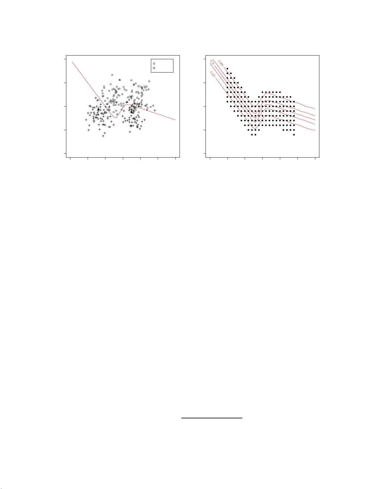
On the Underestimation of Mo del Uncertain t y b y Ba y esian K -nearest Neigh b ors W anh ua Su 1 , Hugh Chi pman 2 , ∗ , Mu Zh u 1 1 Department of Sta tistics and Act uarial Sci ence, Universit y of W aterl oo , W aterlo o, On tario , Canada N2L 3G1 2 Department of Mathem atics and Stati stics, Acadia Uni v ersity , W ol f ville, Nov a Scotia , Canada B4 P 2 R6 No v em b er 23, 2 021 Abstract When using the K -nearest neigh b ors metho d, one often ignores uncertain t y in the c h oi ce of K . T o acc oun t for suc h un ce rtain t y , Holmes and Adams (20 02) prop osed a Ba yesia n f ramew ork for K -n e arest n eig h b ors (KNN). Their Ba ye sian KNN (BKNN) approac h us es a pseudo-lik eliho od function, and sta ndard Mark o v c hain Monte Carlo (MCMC) tec hniques to dr aw p osterior samples. Holmes and Adams (2002) fo cused on th e p erformance of BKNN in terms of misclassification error but did n ot assess its abilit y to quanti fy uncertain t y . W e p resen t some evidence to sho w that BKNN still significan tly un d erestima tes mo del un c ertain t y . Keyw ords : b o otstrap in terv al; MCMC; p osterior interv al; pseu do-l ik elihoo d. 1 In t r o duction The K -nearest neighbors metho d (e.g., Fix and Ho dges 1951; Co v er and Hart 1967) is con- ceptually simple but flexible and useful in practice. It can b e used for b oth r egr ession and classification. W e fo cus on classification o nly . Under the a ssumption that p oin ts close to one another should ha v e similar resp onses, KNN classifies a new observ atio n according to the class lab els of its K nearest neigh b ors. In order to iden tify t he neighbors, one must decide ho w to measure pro ximit y among p oin ts and ho w to define t he neigh b orho o d. The most commonly-used distance metric is t he Eu- clidean distance. The tuning parameter, K , is normally chose n b y cross-v alidatio n. Figure 1 illustrates how KNN works . Supp ose one ta k es K = 5. The p ossible predicted v a lues are { 0 / 5 , 1 / 5 , · · · , 5 / 5 } . Among those fiv e nearest neigh b ors of test p oin t A, four out o f five b elong to class 0. Therefore, A is classified to class 0 with an estimated probabilit y of 4/5. Similarly , test p oin t B is classified to class 1 with a n estimated probability o f 4/5 . ∗ corres p onding author; email: hugh dot chipma n at acadi au do t c a 1 Figure 1: Simulated example illustrating KNN with K = 5. T raining observ ations from class 0 are ind ic ated b y the sym b ol “ ⊕ ”, and those from class 1 are indicated by the symb ol “ • ”. A and B are tw o test p oin ts. Holmes a nd Adams (2002) p oin ted out that regular KNN do es not accoun t for the uncer- tain t y in the c ho ice of K . They presen ted a Ba y esian fra mework for KNN (BKNN), compared its p erformance with the regular KNN on sev eral b enc hmark data sets a nd concluded that BKNN outp erformed KNN in terms o f misclassification error. By mo del a v erag ing ov er the p osterior of K , BKNN is able to improv e predictiv e p erformance. Unfortunately , t hey neve r assesse d the inferen tial asp ec t of BKNN. In this pap er, w e presen t some evidence to sho w that, ev en though BKNN is designed to capture the uncertaint y in the c hoice of K , it still significan tly underestimates ov erall uncertaint y . 2 BKNN W e first giv e a q uic k o v erview of BKNN in the con text of a classification pr o ble m with Q different classes. T o cast KNN in to a Bay esian framework, Holmes and Adams (20 02 ) adopted the following (pseudo) lik eliho o d function for the data: p ( Y | X , β , K ) = n Y i =1 p ( y i | x i , β , K ) = n Y i =1 exp { ( β /K ) P j ∈ N ( x i ,K ) I( y j = y i ) } P Q q =1 exp { ( β /K ) P j ∈ N ( x i ,K ) I( y j = q ) } . (1) The indicator function I is 1 whenev er its argumen t is true, and the notation “ j ∈ N ( x i , K )” iden tifies the indices j o f the K - neares t neigh b ours of x i . Th us P j ∈ N ( x i ,K ) I( y j = y i ) is K times the estimated probability fro m a con v entional KNN mo del. There are t w o unkno wn parameters, K and β . The parameter K is an p ositiv e in te- ger con tro lling the n umber of nearest neigh bo rs; and β is a p ositiv e contin uous parameter go v erning the strength of interaction b et w een a data p oin t and it s neigh b ors. 2 The lik eliho od function (1) is a so-called pseudo-lik eliho o d function (see, e.g., Besag 1974, 1975). Unlik e regular likelih o o d functions, the comp onen t for data p oin t y i dep end s on the class lab els o f o the r data p oin t s y j , for j 6 = i . T reating β and K as r a ndom v aria ble s, the marginal pr edictive distribution for a new data p oin t ( x n +1 , y n +1 ) based on the training data ( X , Y ) is giv en by p ( y n +1 | x n +1 , X , Y ) = X K Z p ( y n +1 | x n +1 , X , Y , β , K ) p ( β , K | X , Y ) dβ , (2) where p ( β , K | X , Y ) ∝ p ( Y | X , β , K ) p ( β , K ) is the p osterior distribution of ( β , K ). Except for the fact that β should b e p ositiv e, little prior knowle dge is known on the lik ely v alues of K and β . Therefore, Holmes and Adams (2002) adopt indep enden t, non- informativ e pr io r densities, p ( β , K ) = p ( β ) p ( K ) where p ( K ) = UNIF[1 , . . . , K max ] with K max = n, p ( β ) = c I( β > 0) , and c is a constant so that p ( β ) is an improp er flat prior on R + . A random-w alk Metrop olis-Hastings algorit hm is t hen used to draw M samples from the p osterior p ( β , K | X , Y ), so that (2) can b e approx imated b y p ( y n +1 | x n +1 , X , Y ) ≈ 1 M M X j =1 p ( y n +1 | x n +1 , X , Y , β ( j ) , K ( j ) ) , (3) where ( K ( j ) , β ( j ) ) is the j th sample f r om the p osterior. 3 Exp erimen ts and results One migh t b eliev e that t he Bay esian form ulation will automatically accoun t for mo del un- certain t y , and that this is a ma jor a dv a n tage of BKNN ov er regula r KNN. W e no w describ e a simple exp erimen t tha t sho ws BKNN still significan tly underestimates mo del uncertaint y . The same exp erimen t is rep eated 100 times. Eac h time, we first generate n = 250 pairs of training data f r om a kno wn, t w o-class mo del (details in Section 3.1). W e then fit BKNN and regular KNN o n the training data, and let them mak e predictions at a set of 160 pre-selected test p oin ts (details in Section 3.2). F or eac h test p oin t, sa y ( x n +1 , y n +1 ), our parameter of in terest is θ n +1 ≡ Pr( y n +1 = 1 | x n +1 ) . (4) W e construct b oth p oin t estimates (Section 3.3) and in t erv a l estimates (Section 3.4) of θ n +1 : ˆ θ n +1 and ˆ I n +1 . T o fit BKNN, w e use the Matlab co de pro vided b y Holmes and Adams (2002) and exactly the same MCMC setting a s described in Holmes and Adams (20 02 , Section 3.1) . T o fit regular K NN , w e use the knn f unc tion in R. 3 −1.5 −1.0 −0.5 0.0 0.5 1.0 1.5 −0.5 0.0 0.5 1.0 1.5 (a) X 1 X 2 Class 1 Class 0 true decision boundary −1.5 −1.0 −0.5 0.0 0.5 1.0 1.5 −0.5 0.0 0.5 1.0 1.5 (b) X 1 X 2 Figure 2 : (a) T rainin g d ata from one exp erimen t, and the tru e probability contour, Pr( y = 1 | x ), as give n b y (5). (b) The fixed set of test p oin ts, and the true probabilit y conto ur. 3.1 Sim ulation Mo del Holmes a nd Adams (2002, Section 3.1 ) illustrated BKNN with a syn thetic data s et consisting of 2 5 0 t r aining and 1000 test p oin ts, tak en from http://www.stats.ox .ac.uk/pub/PRNN . These dat a we re orig ina lly generated from t wo classes, each b eing an equal mixture of t w o biv ariate normal distributions. In order to b e able to generate sligh tly differen t training data ev ery t ime w e rep eat our exp erimen t, w e imitate this synthe tic data set b y assuming the underlying distributions o f class 1 ( C 1 ) and class 0 ( C 0 ) to b e: x | C 1 ∼ f 1 ( x ) = 0 . 5BVN ( µ 11 , Σ ) + 0 . 5BVN ( µ 12 , Σ ) x | C 0 ∼ f 0 ( x ) = 0 . 5BVN ( µ 01 , Σ ) + 0 . 5BVN ( µ 02 , Σ ) , with µ 11 =  − 0 . 3 0 . 7  , µ 12 =  0 . 4 0 . 7  , µ 01 =  − 0 . 7 0 . 3  , µ 02 =  0 . 3 0 . 3  and Σ =  0 . 03 0 0 0 . 03  . The prior class probabilities a r e tak en to b e equal, i.e., Pr( y = 1) = Pr( y = 0) = 0 . 5. Giv en an y data p oint x , its p osterior probability of b eing in C 1 can b e calculated b y Ba y es’ rule Pr( y = 1 | x ) = 0 . 5 f 1 ( x ) 0 . 5 f 1 ( x ) + 0 . 5 f 0 ( x ) . (5) Figure 2(a) sho ws the training data fr o m o ne exp erimen t and the true decision b oundary . 4 3.2 T est p oin ts Instead of f ocusing o n the total misclassification error , w e fo cus on pr edictions made at a fixe d set o f test p oin ts. These test p oin ts are chosen as fo llo ws: first, we lay out a grid along the first co ordinate, X 1 ∈ {− 1 , − 0 . 9 , − 0 . 8 , · · · , 0 . 8 , 0 . 9 } ; for eac h X 1 in that g rid, eight differen t v alues of X 2 are c hosen so that the test p oin ts together “co v er” the critical part of the true p osterior proba bility contour. A to tal of 160 test p oin ts are o bt a ine d this wa y . F ig ure 2( b) sho ws the fixed set of test p oin ts and the tr ue p osterior probability con tour, Pr( y = 1 | x ), as giv en by (5 ). In what follo ws, w e refer to θ n +1 as the key parameter of in terest, but it should b e understo od that the subscript “ n + 1” is used to refer to an y test p oint. There are alto gether 160 suc h test p oin ts, a nd exactly the same calculations are p erformed for all o f them, not just one of them. 3.3 P oin t estimates of θ n +1 F or BKNN, the p oin t estimate of θ n +1 ≡ Pr( y n +1 = 1 | x n +1 ) is the p osterior mean: ˆ θ B K N N n +1 = 1 M M X j =1 Pr( y n +1 = 1 | x n +1 , X , Y , β ( j ) , K ( j ) ) , where ( K ( j ) , β ( j ) ) are samples dra wn from the p osterior distribution, p ( K , β | X , Y ). F or reg- ular KNN, one c ho oses t he parameter K b y cross-v a lidation, and normally uses the origina l KNN score ˜ θ K N N n +1 = 1 K X j ∈ N ( x n +1 ,K ) I( y j = 1) as the p oin t estimate. In order to mak e things fully comparable, ho w ever, we furt he r trans- form the KNN scores by a logistic mo del fitted using the training data. W e describ e this next. Notice that, for binary classification pro blems, i.e., Q = 2, each multiplic ativ e term in (1) can b e rewritten as p ( y i | x i , β , K ) = exp { ( β /K ) P j ∈ N ( x i ,K ) I( y j = y i ) } exp { ( β /K ) P j ∈ N ( x i ,K ) I( y j = y i ) } + exp { ( β /K ) P j ∈ N ( x i ,K ) I( y j 6 = y i ) } ( † ) = exp { ( β /K )[2 P j ∈ N ( x i ,K ) I( y j = y i ) − K ] } 1 + exp { ( β /K )[2 P j ∈ N ( x i ,K ) I( y j = y i ) − K ] } = exp { β [2 g ( y i ) − 1] } 1 + exp { β [2 g ( y i ) − 1] } , (6) where g ( y i ) = 1 K X j ∈ N ( x i ,K ) I( y j = y i ) , (7) is the output of KNN. The step lab elled ( † ) in (6) is due to the identit y X j ∈ N ( x i ,K ) I ( y j = y i ) + X j ∈ N ( x i ,K ) I ( y j 6 = y i ) = K . 5 0.0 0.2 0.4 0.6 0.8 1.0 0.0 0.2 0.4 0.6 0.8 1.0 true value point estimate Regular KNN BKNN θ ^ n + 1 vs θ n + 1 Figure 3: Average of 100 p oin t estimates v ersus the true parameter v alue, f o r all 160 test p oin ts. A 45-degree reference line going through the origin is also display ed. Notice that (6) is equiv alen t to running a logistic regression with no in tercept and [2 g ( y i ) − 1] as the only cov ariat e. Since this extra tra ns formation is built in to BKNN, w e use ˆ θ K N N n +1 = exp { ˆ β [2 ˜ θ K N N n +1 − 1] } 1 + exp { ˆ β [2 ˜ θ K N N n +1 − 1] } (8) as the p oin t estimate of regular KNN in order to b e fully compara ble with BKNN. In ( 8), ˆ β is obtained by running a logistic regression of y i on to [2 g ( y i ) − 1] with no interce pt using the training data . After rep eating the experiment 100 times, w e obtain 10 0 sligh tly differen t p oin t estimates at eac h x n +1 . Figure 3 plots the av erage of these 100 p oin t estimates ag a ins t the true v alue for a ll 160 test p oin ts. W e see that b oth BKNN and regular K NN giv e ve ry similar p oin t estimates. 3.4 In terv al estimates of θ n +1 The main fo cus o f our exp erimen ts is interv al estimation. In particular, w e are in terested in the question of whether these in terv al estimates adequately capture mo del uncertain t y . 6 (a) BKNN coverage probability (%) Frequency 0 20 40 60 80 100 0 5 10 15 95% (b) KNN with Bootstrap coverage probability (%) Frequency 0 20 40 60 80 100 0 20 40 60 80 95% Figure 4 : Estimated co v erage probabilities of (a) ˆ I B K N N n +1 and (b) ˆ I K N N n +1 , for all 160 test p oints. F or BKNN, w e use the 95% p osterior (or credible) interv al as our in terv al estimate, ˆ I B K N N n +1 . This is constructed b y finding the 2 . 5th and 9 7 . 5th p ercen t iles of the p osterior samples. T o obtain an interv al estimate for regula r KNN, ˆ I K N N n +1 , w e resort t o Efron’s b o otstrap. Give n a training set, D , w e generate 500 b o otstrap samples, D ∗ 1 , D ∗ 2 , · · · , D ∗ 500 , and rep eat the entire KNN mo del building pro ces s — that is, c ho osing K by cross-v alidation and calculating ˆ θ n +1 ,b according to (8) — for eve ry D ∗ b , b = 1 , 2 , · · · , 500. The in t e rv al estimate of θ n +1 is constructed by taking the 2 . 5th and 97 . 5 th p erce n tiles of the set, { ˆ θ n +1 , 1 , · · · , ˆ θ n +1 , 500 } . 3.4.1 Co v erage probabilities Our first question of inte rest is: What are the cov erage proba bilitie s of ˆ I K N N n +1 and ˆ I B K N N n +1 ? After rep eating the experiment 100 times, w e obtain 100 slightly differen t interv al estimates at eac h x n +1 . The co v erag e probability of ˆ I B K N N n +1 (and that of ˆ I K N N n +1 ) can b e estimated easily b y coun ting the num b er of times θ n +1 is included in the inte rv al ov er the 1 0 0 exp eri- men ts. Histograms of the estimated cov erage pro babilities for all 160 test p oin ts a re sho wn in Figure 4. The p osterior in terv a ls pro duced b y BKNN can easily b e seen to hav e fairly p o o r cov erage ov erall. 3.4.2 Lengths F or eac h interv al estimate, w e can also calculate its length, e.g., length B K N N n +1 =    ˆ θ B K N N , 97 . 5% n +1 − ˆ θ B K N N , 2 . 5% n +1    , length K N N n +1 =    ˆ θ K N N , 97 . 5% n +1 − ˆ θ K N N , 2 . 5% n +1    . Let length B K N N n +1 and length K N N n +1 7 Figure 5 : Sc hematic illustration of our assessment proto col. V ariation o v er 100 p oin t estimates is used as a b enc hmark to assess the qualit y of the corresp onding int erv al estimates. b e the av erage lengths of these 100 in terv al estimates. Our second question of in t erest is: Are t hey to o long, to o short, or just right? In order to a ns w er this question, we need a “gold standard”. The v ery reason for using these inte rv al estimates is to reflect that there is uncertaint y in our estimate of t he underlying parameter, θ n +1 . This uncertaint y is easy to a s sess directly when one can rep eatedly generate differen t sets of training data and rep eatedly estimate the parameter, whic h is exactly what we hav e done. The standa r d deviations of the 10 0 p oin t estimates (Section 3.3), whic h we write a s std( ˆ θ B K N N n +1 ) and std( ˆ θ K N N n +1 ) , giv e us a direct assessmen t of t his uncertain t y . If the p oin t estimates, ˆ θ B K N N n +1 and ˆ θ K N N n +1 , are approx imately normally distributed, then the corr e ct lengths of the corresp onding interv al estimates should b e roughly 4 times the aforemen tioned standard deviation, that is, length B K N N n +1 ≈ 4 × std( ˆ θ B K N N n +1 ) , (9) length K N N n +1 ≈ 4 × std( ˆ θ K N N n +1 ) . (10) W e use (9)-(10) as heuristic guidelines to assess how w ell the inte rv al estimates can capture mo del uncertain ty , despite la c k of fo r mal justification f o r the norma l appro ximation. Fig ure 5 pro vides a sc hematic illustration of our assessme n t proto col. Figure 6 plots the av erage lengths of these 100 inte rv al estimates a gainst 4 times the standard deviations of the corresp onding p o in t estimates — that is, length B K N N n +1 against 8 0.1 0.2 0.3 0.4 0.5 0.6 0.1 0.2 0.3 0.4 0.5 0.6 4 times the standard deviation of point estimate average length of interval estimate BKNN KNN with Bootstrap length n + 1 vs 4 x std ( θ ^ n + 1 ) slope=1 slope=1/2 Figure 6: Ave rage length of 100 interv al estimates v ersus 4 times the stand ard deviation of the corresp onding p oin t estimate, for all 160 test p oin ts. Two reference lines – b oth going thr ough the origin, one with s lo p e=1 and another with s lo p e=1 / 2 — are also display ed. 4 × std ( ˆ θ B K N N n +1 ) and length K N N n +1 against 4 × std ( ˆ θ K N N n +1 ) — for all 160 test p oin ts. Here, it is easy to see that the Bay esian p osterior in terv als are apparen tly t oo short, whereas b o o ts trapping regular KNN g ives a more accurate a ssessmen t of the amoun t of uncertain t y in the p oin t estimate. 4 Discuss ion Wh y do es BKNN underestimate uncertaint y? W e b eliev e it is b ecause BKNN only accoun ts for the uncertaint y in the numb er of neigh b ors (i.e., the parameter K ), but it is unable to accoun t for the uncertain ty in the spatial lo c ations of these neigh b ors. This is a general phenomenon a sso ciated with pseudo-like liho o d functions. Pseudo-lik eliho o d f unc tions w ere first in tro duced b y Besag (1974, 1 9 75 ) t o mo del spatial in teractions in lattice systems. Since then, they hav e b een widely used in image pro cess - ing (e.g., Besag 198 6 ) and net w o r k tomography (e.g., Strauss and Ik eda 199 0; Liang and Y u 2003; Robins et al. 2 007). Ho we v er, statistical inference ba s ed on pseudo-like liho o d func- 9 tions is still in its infancy . Some researc hers argue that pseudo-likelih o o d inference can b e problematic since it ignores at least part of the dep endenc e structure in the dat a . In appli- cations to mo del so cial net w o rk s, a n um ber of r esearch ers, suc h as W asserman and Ro bins (2005) and Snijders (2 0 02 ), hav e p oin ted out that maxim um pseudo-lik eliho o d estimates are substan tially biased and the standard errors of the parameters a re generally underestimated. F or BKNN, the pseudo-lik eliho o d function (1) clearly ignores the fa c t that the lo cations of one’s neigh b ors are also r a ndom, no t just t he num b er o f neigh b ors. Ho w ev er, for complex net w orks whose full lik eliho o d functions are in tractable, mo dels based on pseudo-likelih o o d are attra c tiv e (if no t the only) alternativ es (Strauss and Ike da 1990). Rather than trying to write do wn t he full lik eliho od functions for these difficult problems, it is probably more fruitful to concentrate our researc h efforts on how to adjust or correct standard error estimates pro duced b y the pseudo-lik eliho o d. T o this effect, one in teresting observ ation from Figure 6 is the fact that length B K N N n +1 ≈ 2 × std( ˆ θ B K N N n +1 ) . If w e con tin ue to use 4 × std( ˆ θ B K N N n +1 ) a s the “gold standard”, then these Bay esian p osterior in terv als are ab out half as long as they should b e. W e hav e observ ed this phenomenon on other examples, to o, but do not y et ha v e an explanation for it. Despite the fact that BKNN seems to underestimate o v erall uncertaint y , that length B K N N n +1 is still a ppro ximately prop ortional to std( ˆ θ B K N N n +1 ) suggests that w e can still rely o n it to assess the r ela t ive uncertaint y o f its predictions. F or many practical problems, this is still v ery useful. F o r example, if tw o a c coun ts, A and B, are b oth predicted to b e fr a udule n t with a high probability of 0 . 9 but the p osterior inte rv al o f A is t wice as long as tha t of B, then it is natural for a financial institution to sp end its limited resources inv estigating a ccount B rather tha n accoun t A. Ac kn owledgmen t This researc h is partially supp orted b y the Natural Science and Engineering R esearch Council (NSER C) of Canada, Canada’s Natio na l Institute for Complex D ata Structures (NICDS) a nd the Mathematics of Info rmation T ec hnology And Complex Systems (MIT ACS) net w o r k . References Besag, J. (197 4). Spatial interaction and the statistical analysis of lattice systems (with discussion). Journal of R oyal Statistic al So ciety: S eries B , 36 (2), 192 –236. Besag, J. (1975) . Statistical analysis of non-lattice data. The Statistician , 24 (3), 17 9–195. Besag, J. (198 6). On the statistical analysis o f dirt y pictures. Journal of R oyal Statistic al So ciety: Series B , 48 (3) , 259–30 2. Co v er, T. and Ha r t , P . (19 67). Nearest neigh b or pattern classification. IEEE T r ansactions on Inform a t ion The ory , IT-13 , 21– 2 7. 10 Fix, E. and Ho dges, J. L. (195 1). Discriminatory analysis–nonparametric discrimination: Consistency prop erties. T echnic al rep ort, USAF School o f Aviation Medicine, Randolph Field, T exas. Holmes, C. C. and Adams, N. M. (2002). A probabilistic nearest neigh b our method for statistical pattern recognition. Journal of R oyal Statistic al S o ciety: Series B , 64 (2), 295– 306. Liang, G. and Y u, B. (2003 ) . Maxim um pseudo lik eliho od estimation in net w ork tomog raph y . IEEE T r ansactions o n Sig n al Pr o c essing , 51 , 20 43–2053. Robins, G., Pattison, P ., Kalish, Y., and L usher, D. (2007 ) . An in tro duction to exp onen tial random graph ( P ∗ ) mo dels for so cial net w orks. So cial Networks , 29 , 173–19 1 . Snijders, T. A. B. (2002). Mark o v chain mon te carlo estimation of exponential random graph mo del. Journal of So cial Structur e , 3 (2 ). Strauss, D. and Ike da, M. ( 1 990). Pseu dolik eliho od estimation f or so cial net w orks. Journal of the A meric an Statistic al Asso ciation , 85 , 204 –212. W a s serman, S. S. and Robins, G. L. (200 5). An in tro duction to random gra phs, dep endence graphs, and p ∗ . In J. S. P . Carrrington and S. S. W a s serman, editors, Mo dels and Metho ds in So cial Network Analysis , pages 148–161. Cambridge Univ ersit y Press, Cam bridge. 11