On Undetected Error Probability of Binary Matrix Ensembles

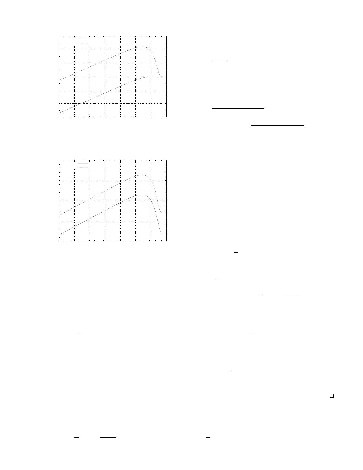
1 On Undetected Error Probability of Binary Matrix Ensembles T adashi W adayama † Abstract — In this paper , an analysis of the undetected erro r probability of en sembles of m × n binary matrices is prese nted. The ensemble called the Bernoulli ensemble whose members are considered as matrices generated from i .i.d. Bernoulli source is mainly c onsidered here. The m ain co ntributions of this work are (i) d eriva tion of the error ex ponent of the ave rage undetected error probability and (ii) closed form expressions f or the variance of the undetected err or probability . It is sho wn th at the b ehav ior of t he exponent for a sparse ensemble is somewhat different from that f or a dense ensemble. Furthermore, as a byproduct of th e proof of the varia nce fo rmula, simple covariance formula of the weight distribution is derived. I . I N T R O D U C T I O N Rando m coding is an extremely powerful tec hnique to sho w the existence of a code satisfy ing certain pr operties. It has been used for proving th e direct part (achiev ability) of many types of c oding theo rems. Recently , the idea of ra ndom coding has also come to be regarded as imp ortant from a practica l point of vie w . An LDPC (Low-density p arity-chec k) cod e can be constructed by choosing a parity c heck matrix from an ensemble of sparse matrices. Thu s, there is a growing interest in ran domly g enerated cod es. One of the main d ifficulties associated with the use of random ly gen erated code s is the difficulty in ev aluating the proper ties or perf ormance o f such codes. For example, it is difficult to e valuate min imum distance, weight d istribution, ML de coding perfor mance, etc. fo r these cod es. T o overcom e this pr oblem, we can take a pr obabilistic ap pr oach . In su ch an approa ch, we consider a n ensem ble of par ity che ck matrices: i.e., pr obability is assigned to eac h matrix in the ensemble. A proper ty of a matrix (e.g., minimum distance, weight distributions) can then be regarded as a rando m variable. It is natu ral to co nsider statistics of the ran dom variable such as mean, variance, higher m oments and covariance. In some cases, we can show that a prop erty is stro ngly con centrated around its e xpectation. Such a conce ntration result ju stifies the use of th e proba bilistic approac h. Recent advances in th e analysis of th e average weigh t distributions of LDPC codes, such as those described by Litsyn and Shev elev [4][5], Burshtein and Mill er [6], Richardson and Urbanke [9], sho w that the probabilistic ap proach is a useful technique fo r investigating typ ical pro perties of codes and matrices, wh ich are not easy to obtain. Furth ermore, th e second m oment an alysis of th e weig ht d istribution of LDPC codes [ 7][8] can be utilized to prove concentratio n results for weight distributions. † Nago ya Institute of T echnology , email:wada yama@nit ech.ac.jp. A part of this work was prese nted at IT A w orkshop in UC SD, Feb. 2007. The evaluation of the err or detectio n pro bability of a given code (or given parity check matrix ) is a classical pro blem in coding theory [2], [3] and some results on this topic have been der iv ed from the v iew point o f a pr obabilistic app roach. For e xample, for a linea r code ensemb le the inequality , P U < 2 − m has long been known where P U is the undetected error probab ility and m is the nu mber o f rows of a parity check matrix. Since the undetected error prob ability can be e xpressed as a linear com bination of the weight d istribution o f a code, there is a natural co nnection between the expe ctation of the weight distrib ution an d th e e xpectation of the u ndetected error probab ility . In t his paper , an analysis of the undetected err or probability of ensemb les of binar y matrices of size m × n is presented. An er ror d etection schem e is a cru cial p art o f a feedback er ror correction sch eme such as ARQ(Au tomatic Repeat reQuest). Detailed knowledge of the erro r detectio n perfor mance of a matrix ensem ble would be u seful for assessing the perfor- mance of a feedba ck error correction scheme. I I . A V E R AG E U N D E T E C T E D E R RO R P RO B A B I L I T Y A. Notation For a g iv e n m × n ( m, n ≥ 1) binary parity check matrix H , let C ( H ) be the binary linea r code of length n defined by H , n amely , C ( H ) △ = { x ∈ F n 2 : H x t = 0 m } where F 2 is the Galois field with two elements { 0 , 1 } ( the addition over F 2 is denoted by ⊕ ). Th e notation 0 m denotes the zero v ector of leng th m . In this paper, a boldface letter , such as x fo r example, d enotes a bin ary r ow vector . Throu ghout the paper, a binary sy mmetric ch annel (BSC) with crossover p robab ility ǫ ( 0 < ǫ < 1 / 2 ) is assumed. W e assume the conv entional scenario f or error d etection: A transmitter send s a codeword x ∈ C ( H ) to a receiver via a BSC with crossover p robab ility ǫ . Th e r eceiver obtains a received word y = x ⊕ e , where e deno tes an er ror vector . The receiver firstly co mputes the s yndro me s = H y t and then checks whethe r s = 0 m holds or n ot. An undetected error event oc curs when H e t = 0 m and e 6 = 0 m . This me ans that th e error vector e ∈ C ( e 6 = 0 n ) causes an undetected erro r event. Th us, the undetected error probab ility P U ( H ) can be expressed as P U ( H ) = X e ∈ C ( H ) , e 6 =0 m ǫ w ( e ) (1 − ǫ ) n − w ( e ) (1) where w ( x ) d enotes the Hamming w eight of vector x . The 2 above equatio n ca n be r ewritten as P U ( H ) = n X w =1 A w ( H ) ǫ w (1 − ǫ ) n − w , (2) where A w ( H ) is d efined by A w ( H ) △ = X x ∈ Z ( n,w ) I [ H x t = 0 m ] . (3) The set { A w ( H ) } n w =0 is usually called the weight distrib ution of C ( H ) . T he n otation Z ( n,w ) denotes the set of n -tu ples with weight w . The n otation I [ condition ] is the indica tor function such that I [ conditi on ] = 1 if condition is true; other wise, it ev aluates to 0 . Suppose that G is a set o f binary m × n matrices ( m, n ≥ 1) . Note tha t G may contain som e matric es with all elemen ts identical. Such ma trices should be distingu ished as distinct matrices. A prob ability P ( H ) is associated with each matrix H in G . T hus, G can be con sidered as an en semble o f binary matrices. Let f ( H ) be a real-valued fun ction which depend s on H ∈ G . Th e expectatio n of f ( H ) with respect to the ensemble G is defined by E G [ f ( H )] △ = X H ∈G P ( H ) f ( H ) . (4) The av erage weight distribution of a gi ven ensemble G is given by E G [ A w ( H )] . This quantity is very usef ul for a nalyzing the perfor mance of b inary linea r cod es, inclu ding ana lysis of the undetected erro r p robab ility . B. Bernou lli en semble In this paper, we will fo cus on a parameter ized ensemble B m,n,k which is called the Bernoulli ensemble b ecause the Bernoulli ensem ble is amen able to ensemble an alysis. The Bernoulli ensemb le B m,n,k contains all th e bin ary m × n matrices ( m, n ≥ 1 ), whose elem ents are regar ded as i.i. d. binary rand om variables such th at an elem ent takes the value 1 with pr obability p △ = k /n . The pa rameter k (0 < k ≤ n/ 2 ) is a positi ve real nu mber w hich rep resents th e average nu mber of ones for each row . In other words, a ma trix H ∈ B m,n,k can b e co nsidered as an o utput f rom the Bernoulli sou rce such that symb ol 1 occur s with probability p . From the above definition , it is clear th at a matrix H ∈ B m,n,k is associated with the pr obability P ( H ) = p ¯ w ( H ) (1 − p ) mn − ¯ w ( H ) , (5) where ¯ w ( H ) is the num ber of ones in H (i.e., Ham ming weight of H ). The average weight distribution of the Bern oulli ensemble is g iv en by E B m,n,k [ A w ( H )] =  1 + z w 2  m  n w  (6) for w ∈ [0 , n ] where z △ = 1 − 2 p . The notation [ a, b ] deno tes the set o f consecu tiv e integers from a t o b . Th e average weight distribution of this ensemble was first discussed by Lits yn and Shevele v [4]. If k is a constant (i.e., not a function of n ), this ensemble can be considered as an ensem ble of sparse matrices. In the spacial case where k = n/ 2 , equal probability 1 / 2 mn is assigned to every m atrix in the Bern oulli ensem ble. As a simplified notation, we will d enote R m,n △ = B m,n,n/ 2 , wh ere R m,n is called the rando m ensemb le . Sin ce a ty pical instance o f R m,n contains Θ( mn ) on es, the ensemble can be regarded as an ensemble of d ense matrices. C. A v erag e und etected err or pr o bability of an ensemble For a giv en m × n matrix H , the e valuation of the undetected error pro bability P U ( H ) is in gen eral compu tationally dif ficu lt because we need to know the weigh t distribution of C ( H ) for such e valuation. On the othe r hand , in som e cases, we can ev alu ate the av erage of P U ( H ) fo r a g iv en ensemble. Such an av erage pr obability is useful for the estimation o f the undete cted error pr obability o f a matrix which belo ngs to the ensemble. T aking the ensem ble average of the undetected er ror pr ob- ability over a giv en en semble G , we have E G [ P U ( H )] = E G " n X w =1 A w ( H ) ǫ w (1 − ǫ ) n − w # = n X w =1 E G [ A w ( H )] ǫ w (1 − ǫ ) n − w . (7) In the above equation s, H can b e regard ed as a r andom variable. From this equ ation, it is evident that the average of P U ( H ) can be evaluated if we kn ow the average weight distribution of the en semble. For examp le, in the case of the random ensemb le R m,n , th e av e rage u ndetected er ror probab ility has a simple closed form. Lemma 1: Th e average u ndetected er ror probab ility of the random ensemble R m,n is given by E R m,n [ P U ( H )] = 2 − m (1 − (1 − ǫ ) n ) . (8) (Proof) By using (7), we h ave E R m,n [ P U ( H )] = n X w =1 E R m,n [ A w ( H )] ǫ w (1 − ǫ ) n − w = n X w =1 2 − m  n w  ǫ w (1 − ǫ ) n − w = 2 − m (1 − (1 − ǫ ) n ) . (9) The second equality is ba sed on the well known result [1]: E R m,n [ A w ( H )] = 2 − m  n w  . ( 10) The last equ ality is du e to the b inomial theo rem. D. Err or exponent o f undetected err or pr obab ility For a given sequence of (1 − R ) n × n matr ix ensemb les ( n = 1 , 2 , 3 , . . . , ) , the av erage u ndetected err or prob ability is usually an exponen tially decr easing func tion of n , whe re R is a real numb er satisfying 0 < R < 1 (called the d esign rate ). Thu s, the e x ponen t of the undetected err or pr obability is of prime impor tance in understand ing the as ymptotic b ehavior of the undetected e rror pr obability . 3 1) Definitio n of err or exponen t: Let {G n } n> 0 be a series of ensembles such that G n consists of (1 − R ) n × n binar y matrices. In order to see the asymptotic behavior of the undetected erro r p robab ility of this seq uence of ensemb les, it is reasonab le to d efine the erro r expo nent of und etected error probab ility in th e following way: Definition 1: Th e asymptotic error e x ponen t of the average undetected error probability for a series of ensembles {G n } n> 0 is defined b y T G n △ = lim n →∞ 1 n log 2 E G n [ P U ] (11) if the limit exists. Hencefor th we will n ot explicitly express the dep endenc e o f P U on H , writing instead P U to d enote P U ( H ) in all cases where there is no fear o f con fusion. The following examp le describes the exp onent of th e r an- dom ensem ble. Example 1: Conside r th e series of the ran dom ensembles {R n, (1 − R ) n } n> 0 . It is easy to evaluate T R (1 − R ) n,n : T R (1 − R ) n,n = lim n →∞ 1 n log 2 E R (1 − R ) n,n [ P U ] = lim n →∞ 1 n log 2 2 − (1 − R ) n (1 − (1 − ǫ ) n ) = − (1 − R ) . (12) This equality im plies that the average undetected error pro ba- bility of the sequence of random ensembles beh av es like E R (1 − R ) n,n [ P U ] ≃ 2 − n (1 − R ) (13) if n is sufficiently large. Note that the expon ent − (1 − R ) is indepen dent fro m th e crossover p robab ility ǫ . 2) Err or exponent a nd a symptotic gr o wth rate: The asymp - totic gr owth r ate of the a verage weig ht distribution ( for simplicity henc eforth abbreviated as the a symptotic growth rate), which is the basis of the de riv ation of the err or exponent, is defined a s follows. Definition 2: Sup pose th at a series of ensem bles {G n } n> 0 is given. If lim n →∞ 1 n log 2 E G n [ A ℓn ] exists for 0 ≤ ℓ ≤ 1 , th en we define th e asymptotic g r owth rate f ( ℓ ) b y f ( ℓ ) △ = lim n →∞ 1 n log 2 E G n [ A ℓn ] . (14) The param eter ℓ is called the normalized weig ht . From this d efinition, it is clear that E G n [ A ℓn ] = 2 n ( f ( ℓ )+ o (1)) , (15) where the notation o (1) deno tes terms which c onv e rge to 0 in the limit as n goes to infinity . The asymp totic growth rate of some en sembles of b inary matrices can be foun d in [4][5][ 6]. The next theo rem gives the error expon ent of the u ndetected error prob ability for a ser ies of en sembles {G n } n> 0 . Theor em 1: The er ror exponent of {G n } n> 0 is given by T G n = sup 0 <ℓ ≤ 1 [ f ( ℓ ) + ℓ log 2 ǫ + (1 − ℓ ) log 2 (1 − ǫ )] , (16 ) where f ( ℓ ) is the asymptotic g rowth rate o f {G n } n> 0 . (Proof) Based on the definition of asympto tic growth rate, we can rewrite T G n in the fo rm T G n = lim n →∞ 1 n log 2 E G n [ P U ] = lim n →∞ 1 n log 2 n X w =1 E G n [ A w ] ǫ w (1 − ǫ ) n − w = lim n →∞ 1 n log 2 n X w =1 2 n ( f ( w n )+ K ( ǫ,n,w )+ o (1)) , where K ( ǫ, n, w ) is defin ed by K ( ǫ, n, w ) △ = w n log 2 ǫ +  1 − w n  log 2 (1 − ǫ ) . (17) Using a c onv e ntional tech nique for b ound ing summation, w e have the following u pper bou nd on T G n : T G n = lim n →∞ 1 n log 2 n X w =1 2 n ( f ( w n )+ K ( ǫ,n,w )+ o (1)) ≤ lim n →∞ 1 n log 2 n n max w =1 2 n ( f ( w n )+ K ( ǫ,n,w )+ o (1)) = lim n →∞ n max w =1 1 n log 2 2 n ( f ( w n )+ K ( ǫ,n,w )+ o (1)) = lim n →∞ n max w =1 h f  w n  + K ( ǫ, n, w ) + o (1) i = sup 0 <ℓ ≤ 1 [ f ( ℓ ) + ℓ log 2 ǫ + (1 − ℓ ) log 2 (1 − ǫ )] . (18 ) W e can also show that T G n is grea ter th an or equal to th e right-ha nd side of the ab ove ineq uality (1 8) in a similar manner . This mean s th at the rig ht-hand side of the ineq uality is asympto tically tigh t. The next example discusses the case of the random ensem- ble. Example 2: Let us ag ain consid er the series of th e ran dom ensembles given b y {R (1 − R ) n,n } n> 0 . These ensembles have the asymptotic growth rate f ( ℓ ) = h ( ℓ ) − (1 − R ) , where the function h ( x ) is the binar y entropy f unction defined by h ( x ) △ = − x log 2 x − (1 − x ) log 2 (1 − x ) . (19) In this case, by using Theorem 1, we have T R (1 − R ) n,n = sup 0 <ℓ ≤ 1 [ h ( ℓ ) − (1 − R ) + ℓ log 2 ǫ + (1 − ℓ ) lo g 2 (1 − ǫ )] . (20) Let D ℓ,ǫ △ = ℓ log 2  ℓ ǫ  + (1 − ℓ ) log 2  1 − ℓ 1 − ǫ  . (21) By using D ℓ,ǫ , we can rewrite (2 0) as T R (1 − R ) n,n = sup 0 <ℓ ≤ 1 [ − (1 − R ) − D ℓ,ǫ ] . (22) Since D ℓ,ǫ can be con sidered as the Kullback -Libler diver - gence betwee n two prob ability distributions ( ǫ, 1 − ǫ ) an d ( ℓ, 1 − ℓ ) , D ℓ,ǫ is always non -negative and D ℓ,ǫ = 0 hold s if and only if ℓ = ǫ . Thus, we o btain sup 0 <ℓ ≤ 1 [ − (1 − R ) − D ℓ,ǫ ] = − (1 − R ) , (23) 4 which is identica l to the expo nent ob tained in expression (12). Let g ( r nd ) ǫ ( ℓ ) △ = h ( ℓ ) − (1 − R ) + ℓ log 2 ǫ + (1 − ℓ ) log 2 (1 − ǫ ) . Figure 1 displays the beha v ior of g ( r nd ) ǫ ( ℓ ) wh en R = 0 . 5 . This figur e confir ms th e r esult th at th e m aximum ( sup 0 <ℓ ≤ 1 g ( r nd ) ǫ ( ℓ ) = − 0 . 5 ) is attained at ℓ = ǫ . -1 -0.9 -0.8 -0.7 -0.6 -0.5 -0.4 0 0.1 0.2 0.3 0.4 0.5 g ε (rnd) (l) Normalized weight ε =0.4 ε =0.2 ε =0.1 The curves of g ( rnd ) ǫ ( ℓ ) correspond to the parameters ǫ = 0 . 1 , 0 . 2 , 0 . 4 from left t o ri ght are presented. As a reference, li ne of − (1 − R ) = − 0 . 5 is also included in the figu re. Fig. 1. T he curves of g ǫ ( ℓ ) for random ensembles w ith R = 0 . 5 . E. Err or exponen t o f the Bern oulli e nsemble with co nstant k The asy mptotic growth rate o f the Bernoulli ensemble B m,n,k with a con stant k an d design rate R is given by f ( ℓ ) = h ( ℓ ) + (1 − R ) lo g 2  1 + e − 2 kℓ 2  . (24) This for mula is presen ted in [4]. T he err or exponent of this ensemble shows a different b ehavior fr om that for random ensembles. Example 3: Conside r the Bernoulli ensemble with parame - ters R = 0 . 5 and k = 20 . Let g ( spm ) ǫ ( ℓ ) △ = H ( ℓ ) + (1 − R ) log 2  1 + e − 2 kℓ 2  + ℓ log 2 ǫ + (1 − ℓ ) lo g 2 (1 − ǫ ) . (25) Figure 2 in cludes the curves of g ( spm ) ǫ ( ℓ ) where ǫ = 0 . 1 , 0 . 2 , 0 . 4 . In co ntrast to g ( r nd ) ǫ ( ℓ ) o f a ra ndom ensem ble, we can see that g ( spm ) ǫ ( ℓ ) is no t a co ncave function . The shape of t he c urve o f g ( spm ) ǫ ( ℓ ) dep ends on the cro ssover probability ǫ . For large ǫ , g ǫ ( ℓ ) takes its largest value aroun d ℓ = ǫ . On the other hand , for small ǫ , g ( spm ) ǫ ( ℓ ) has the supr emum at ǫ = 0 . Figure 3 presents the e rror expo nent of Bernoulli ensembles with parameters R = 0 . 3 , 0 . 5 , 0 . 7 , 0 . 9 and k = 20 . As an example, consider the exponen t for R = 0 . 5 . In the regime where ǫ is smaller than (arou nd) 0 .3, the erro r expo nent is a monoto nically decr easing function of ǫ . The examples sug gest th at a sparse ensemble has less powerful error detection perfo rmance than tha t of a d ense ensemble (such as th e random ensemble) in term s of th e error exponent. Howe ver, if th e cro ssover probability is sufficiently large, th e dif f erence in exponen t of sparse and dense ensembles -1 -0.8 -0.6 -0.4 -0.2 0 0 0.1 0.2 0.3 0.4 0.5 g ε (spm) (l) Normalized weight ε =0.4 ε =0.2 ε =0.1 The curves of g ( spm ) ǫ ( ℓ ) correspond to the parameters ǫ = 0 . 1 , 0 . 2 , 0 . 4 are presented. The p arameters R = 0 . 5 , k = 20 are assumed. As a reference, l ine of − (1 − R ) = − 0 . 5 i s also inclu ded in t he figure. Fig. 2. T he curves of g ( spm ) ǫ ( ℓ ) for Berno ulli en sembles. -0.8 -0.7 -0.6 -0.5 -0.4 -0.3 -0.2 -0.1 0 0 0.1 0.2 0.3 0.4 0.5 Error exponent Crossover probability ε R=0.3 R=0.5 R=0.7 R=0.9 The curves of T B m,n,k correspond t o th e parameters R = 0 . 3 , 0 . 5 , 0 . 7 , 0 . 9 and k = 20 . are presented. Fig. 3. E rror expone nt of Bernoulli ense mble. is negligible. For example, the exponen t of the Bernoulli ensemble in Fig. 3 is a lmost equal to th at of the rando m ensemble when ǫ is larger than ( around ) 0.3. The above prope rties of the error exponents of the Berno ulli ensembles can be explain ed with refer ence to their average weight d istributions (o r asymptotic gr owth rate). Figure 4 displays the asym ptotic growth rates of a ran dom ensemble and a Ber noulli ensemble. The weigh t of typical err or vectors is very close to ǫn when n is sufficiently large. For a large v alu e of ǫ , such as ǫ = 0 . 4 , the average weight distribution aroun d w = 0 . 4 n , namely E G [ A 0 . 4 n ] , do minates the undetected error pr obability . In su ch a rang e, th e difference in the av erage weight distributions correspo nding to th e ran dom and the Bernoulli en sembles is small. On the other hand, if th e crossover prob ability is small, weight distributions of low weight bec ome the m ost influen tial parameter . The difference in the average weig ht distributions of small weig ht results in a difference in the erro r expo nent. Note th at th e time complexity o f th e er ror detection op- eration (multiplication of rec eiv ed vector and a par ity c heck 5 -0.4 -0.2 0 0.2 0.4 0.6 0 0.05 0.1 0.15 0.2 0.25 0.3 Asymptotic growth rate Normalized weight Random ensemble (R=0.5) Sparse matrix ensemble (R=0.5, k=20) Fig. 4. Asymptotic gro wth rate of a random ensemble and a Bernoull i ensemble. matrix) is O ( n 2 ) -time for a typ ical instance of a random en- semble, and is O ( n ) -time for a typical instance of a Berno ulli ensemble with con stant k . A spar se matrix o ffers almost same error d etection p erform ance of a dense m atrix w ith linea r time complexity if ǫ is sufficiently large. I I I . V A R I A N C E O F U N D E T E C T E D E R R O R P R O BA B I L I T Y In the previous section, we ha ve seen that the av erage weight distribution plays an important role in the deriv a tion of a verage undetected error p robab ility . Similar ly , we need to examine the cova riance of weig ht d istrib ution in orde r to analyze the variance of u ndetected error pr obability . A. Covariance formula The covariance between two real-v alu ed fun ctions f ( · ) , g ( · ) defined on an ensemble G is giv en by Cov G [ f , g ] △ = E G [ f g ] − E G [ f ] E G [ g ] . (26) The next theor em for ms the b asis o f th e deriv atio n of the variance of the und etected erro r pr obability fo r the Bern oulli ensemble. The covariance of the weight distribution fo r the Bernoulli ensem ble is given in the f ollowing theor em. Theor em 2: The covariance of the weight distribution f or the Berno ulli en semble B m,n,k is given by Cov B m,n,k ( A w 1 , A w 2 ) △ =  1 + z w 1 2  m  1 + z w 2 2  m × w 1 X v =m ax { 0 ,w 1 + w 2 − n }  n w 1  w 1 v  n − w 1 w 2 − v  ×  1 + z w 1 + w 2 − 2 v − z w 1 + w 2 (1 + z w 1 )(1 + z w 2 )  m − 1  (27) for 1 ≤ w 1 ≤ w 2 ≤ n and Cov B m,n,k ( A w 1 , A w 2 ) = Co v B m,n,k ( A w 2 , A w 1 ) (28) for 1 ≤ w 2 < w 1 ≤ n where z = 1 − 2 p and p = k /n . (Proof) See Appendix . Remark 1: When k = n/ 2 , B m,n,k becomes th e r andom ensemble R m,n . W e discu ss this case here. W e first assume that 1 ≤ w 1 ≤ w 2 ≤ n . Let p = 1 / 2 (i.e., k = n/ 2 ) . In such a ca se, we have z = 1 − 2 p = 0 . Define L by L △ =  1 + z w 1 + w 2 − 2 v − z w 1 + w 2 (1 + z w 1 )(1 + z w 2 )  . (29 ) The variable L takes the following values: L =    1 , w 1 < w 2 1 , w 1 = w 2 , v < w 1 2 , w 1 = w 2 , v = w 1 . (30) Substituting z = 0 in to equation (27) and using th e identity (28), we g et Cov R m,n ( A w 1 , A w 2 ) =  0 , 1 ≤ w 1 6 = w 2 ≤ n 2 − 2 m  n w  (2 m − 1) , 1 ≤ w 1 = w 2 ≤ n. (31) Another pro of o f this fo rmula is presen ted in [10]. B. V ariance of undetected err or pr obab ility The v arian ce of the undetected er ror probability is a straight- forward conseque nce of Th eorem 2. Cor ollary 1 : The variance o f th e un detected er ror p robabil- ity of th e Bernoulli en semble, σ 2 B m,n,k is given by σ 2 B m,n,k = n X w 1 =1 n X w 2 =1 Cov B m,n,k ( A w 1 , A w 2 ) × ǫ w 1 + w 2 (1 − ǫ ) 2 n − w 1 − w 2 . (32) (Proof) The variance of the und etected err or probability P U is giv en b y σ 2 B m,n,k = E B m,n,k [( P U − µ ) 2 ] = E B m,n,k [ P 2 U ] − E B m,n,k [ P U ] 2 . (33) W e first consider the second mome nt of the un detected error probab ility: E B m,n,k [ P 2 U ] = E B m,n,k   n X w =1 A w ǫ w (1 − ǫ ) n − w ! 2   = E B m,n,k " n X w 1 =1 n X w 2 =1 A w 1 A w 2 ǫ w 1 + w 2 (1 − ǫ ) 2 n − w 1 − w 2 # = n X w 1 =1 n X w 2 =1 E B m,n,k [ A w 1 A w 2 ] ǫ w 1 + w 2 (1 − ǫ ) 2 n − w 1 − w 2 . (34) The square d average un detected error pr obability can be expressed as E B m,n,k [ P U ] 2 = E B m,n,k " n X w =1 A w ǫ w (1 − ǫ ) n − w !# 2 = n X w 1 =1 n X w 2 =1 E B m,n,k [ A w 1 ] E B m,n,k [ A w 2 ] × ǫ w 1 + w 2 (1 − ǫ ) 2 n − w 1 − w 2 . (35) 6 Combining the se equalities and the c ovariance of the weight distribution, th e variance of und etected error p robab ility σ 2 B m,n,k is ob tained. Remark 2: Th e cov ariance of the weight distribution fo r a giv en e nsemble B m,n,k is u seful not o nly for th e evaluation of the variance of P U . Let X b e a ran dom variable represen ted by X = n X w =0 α ( w ) A w , (36) where α ( w ) is a re al-valued f unction of w . T he covariance of the weight distribution is required mor e g enerally for the ev aluatio n o f the variance of X , which is given by σ 2 X = n X w 1 =0 n X w 2 =0 Cov B m,n,k ( A w 1 , A w 2 ) α ( w 1 ) α ( w 2 ) . (37) A specialized version ( the case whe re X = P U ) of th is equation has been derived in the pr evious coro llary . Example 4: Let us consider th e Bern oulli ensem ble w ith m = 1 , n = 2 and k = 1 / 2( p = 1 / 4) . T ab le I displays the weight distributions and und etected erro r p robabilities for the 4 matr ices in B 1 , 2 , 1 / 2 . T ABLE I W E I G H T D I S T R I B U T I O N S A N D U N D E T E C T E D E R RO R P R O BA B I L I T I E S H C ( H ) A 1 ( H ) A 2 ( H ) P U ( H ) (0,0) { 00 , 01 , 10 , 11 } 2 1 2 ǫ − ǫ 2 (0,1) { 00 , 10 } 1 0 ǫ − ǫ 2 (1,0) { 00 , 01 } 1 0 ǫ − ǫ 2 (1,1) { 00 , 11 } 0 1 ǫ 2 From the definition of a Bern oulli ensemb le, the f ollow- ing p robab ility is assigned to each matr ix: P ((0 , 0)) = 9 / 16 , P ((0 , 1)) = 3 / 16 , P ((1 , 0)) = 3 / 16 , P ((1 , 1)) = 1 / 16 . Combining th e undetecte d error p robab ilities presented in T able I and the abov e pr obability assignm ent, we immediately have the first and second mo ments: E B 1 , 2 , 1 / 2 [ P U ] = 2 3 ǫ − 7 8 ǫ 2 (38) E B 1 , 2 , 1 / 2 [ P 2 U ] = 21 8 ǫ 2 − 3 8 ǫ 3 + ǫ 4 . (39) From these moments, the variance can be d erived: σ 2 B 1 , 2 , 1 / 2 = E B 1 , 2 , 1 / 2 [ P 2 U ] − E B 1 , 2 , 1 / 2 [ P U ] 2 = 3 8 ǫ 2 − 3 8 ǫ 3 + 15 64 ǫ 4 . (40) W e can also consider anoth er rou te to de riv e the variance by usin g Coro llary 1. Th e covariances of B 1 , 2 , 1 / 2 are given by Cov B 1 , 2 , 1 / 2 (1 , 1) = 3 / 8 (41) Cov B 1 , 2 , 1 / 2 (1 , 2) = C ov B 1 , 2 , 1 / 2 (2 , 1) = 3 / 16 (42) Cov B 1 , 2 , 1 / 2 (2 , 2) = 1 5 / 64 . (43) From Corollar y 1 , we ob tain the variance σ 2 B 1 , 2 , 1 / 2 = 2 X w 1 =1 2 X w 2 =1 Cov B m,n,k ( A w 1 , A w 2 ) × ǫ w 1 + w 2 (1 − ǫ ) 4 − w 1 − w 2 = (3 / 8) ǫ 2 (1 − ǫ ) 2 + (3 / 16) ǫ 3 (1 − ǫ ) + (3 / 16) ǫ 3 (1 − ǫ ) + (15 / 64) ǫ 4 = 3 8 ǫ 2 − 3 8 ǫ 3 + 15 64 ǫ 4 , that is id entical to expression (40). In the ca se of k = n/ 2 (i.e. the case of a r andom ensem ble), we can d erive a closed for m expression for the variance. Cor ollary 2 : For the rand om ensemble R m,n , the variance of the undetected e rror pr obability P U is given by σ 2 R m,n = (1 − 2 − m )2 − m  ( ǫ 2 + (1 − ǫ ) 2 ) n − (1 − ǫ ) 2 n  . (44) (Proof) The variance of un detected erro r p robab ility σ 2 R m,n can be ob tained in the following way: σ 2 R m,n = E R m,n [ P 2 U ] − E R m,n [ P U ] 2 = n X w 1 =1 n X w 2 =1 Cov R m,n [ A w 1 , A w 2 ] ǫ w 1 + w 2 (1 − ǫ ) 2 n − w 1 − w 2 = n X w =1 (1 − 2 − m )2 − m  n w  ǫ 2 w (1 − ǫ ) 2 n − 2 w . The second equality is d ue to Co rollary 1. The last equality are du e to Eq. (31). W e can f urther simp lify the expression using the bin omial theor em: σ 2 R m,n = (1 − 2 − m )2 − m n X w =0  n w  ( ǫ 2 ) w ((1 − ǫ ) 2 ) n − w − (1 − 2 − m )2 − m (1 − ǫ ) 2 n = (1 − 2 − m )2 − m ×  ( ǫ 2 + (1 − ǫ ) 2 ) n − (1 − ǫ ) 2 n  . (45 ) The last equ ality is the claim of the theorem. The next example facilitates an under standing of how th e av erage and the variance of P U behave. Example 5: W e con sider the rand om ensemble with m = 20 , n = 40 , and the Bernou lli ensemble with m = 20 , n = 40 , k = 5 (lab eled ”Sparse” in Fig. 5 ). Figure 5 dep icts the av erage undetected error p robab ilities of the two ensembles. It can b e obser ved that the average undetected erro r p roba- bility of the r andom en semble mono tonically d ecreases as ǫ decreases. In contrast, the curve for the B ernoulli ensemble has a peak around ǫ ≃ 0 . 025 . Figure 6 shows the variance of P U for the above two ensemb les. The two cu rves h av e a similar shape, but the v arian ce of th e spar se ensemb le is al ways lar ger than that of the rand om ensemble. C. Asymptotic beha vior W e her e discuss the asymp totic behavior of th e covariance of the weigh t d istribution and the variance of P U for the Bernoulli ensemble. T he following coro llary exp lains the 7 10 -12 10 -10 10 -8 10 -6 10 -4 10 -2 10 0 10 -7 10 -6 10 -5 10 -4 10 -3 10 -2 10 -1 10 0 Mean Crossover probability ε Random Sparse Random ensemble: m = 20 , n = 40 , Sparse matrix ensemble: m = 20 , n = 40 , k = 5 . Fig. 5. A verage undetected error probabilit ies. 10 -20 10 -15 10 -10 10 -5 10 0 10 -7 10 -6 10 -5 10 -4 10 -3 10 -2 10 -1 10 0 Variance Crossover probability ε Random Sparse Random ensemble: m = 20 , n = 40 , Sparse matrix ensemble: m = 20 , n = 40 , k = 5 . Fig. 6. V ariance of undete cted error probabili ty . asymptotic b ehavior o f th e covariance of the weigh t distri- bution. Cor ollary 3 : Let th e asymp totic gr owth rate of th e covari- ance of th e weigh d istribution o f the Bern oulli ensemble be T ( ℓ 1 , ℓ 2 ) defined by T ( ℓ 1 , ℓ 2 ) △ = lim n →∞ 1 n log 2 Cov B (1 − R ) n,n,k ( A ℓ 1 n , A ℓ 2 n ) (46) for 0 < ℓ 1 , ℓ 2 ≤ 1 an d 0 < R ≤ 1 . The asympto tic gr owth rate is g iv en b y T ( ℓ 1 , ℓ 2 ) = sup max { 0 ,ℓ 1 + ℓ 2 − 1 }≤ ν ≤ ℓ 1 Q ( ν ) (47) for 0 < ℓ 1 ≤ ℓ 2 ≤ 1 and T ( ℓ 1 , ℓ 2 ) = T ( ℓ 2 , ℓ 1 ) (48) for 0 < ℓ 2 < ℓ 1 ≤ 1 where Q ( ν ) is d efined by Q ( ν ) △ = − 2(1 − R ) + h ( ℓ 1 ) + h  ν ℓ 1  + h  ℓ 2 − ν 1 − ℓ 1  + sup 0 <µ ≤ 1 − R α ( µ, ν ) . (4 9) The fun ction α ( µ, ν ) is defined by α ( µ, ν ) △ = h  µ 1 − R  + µ log 2  e − 2 k ( ℓ 1 + ℓ 2 − 2 ν ) − e − 2 k ( ℓ 1 + ℓ 2 )  + (1 − R − µ ) log 2  (1 + e − 2 kℓ 1 )(1 + e − 2 kℓ 2 )  . (50) (Proof) W e h ere r ewrite the covariance fo rmula (2 7) into asymptotic form . By using the Binomial theorem , we have  1 + z w 1 + w 2 − 2 v − z w 1 + w 2 (1 + z w 1 )(1 + z w 2 )  m − 1 = m X i =1  m i   z w 1 + w 2 − 2 v − z w 1 + w 2 (1 + z w 1 )(1 + z w 2 )  i . (51) By using this identity , the covariance in ( 27) can be r ewritten in the fo llowing form : Cov B m,n,k ( A w 1 , A w 2 ) = 2 − 2 m w 1 X v =m ax { 0 ,w 1 + w 2 − n }  n w 1  w 1 v  n − w 1 w 2 − v  Θ , where Θ is defined by Θ △ = m X i =1  m i   z w 1 + w 2 − 2 v − z w 1 + w 2  i × ((1 + z w 1 )(1 + z w 2 )) m − i . (52) Letting w 1 = ℓ 1 n, w 2 = ℓ 2 n, v = ν n, m = (1 − R ) n , we have lim n →∞ 1 n log 2 2 − 2 m = − 2(1 − R ) (53) and lim n →∞ 1 n log 2  n w 1  w 1 v  n − w 1 w 2 − v  = h ( ℓ 1 ) + h  ν ℓ 1  + h  ℓ 2 − ν 1 − ℓ 1  . (54) If k is a constant and 0 ≤ ℓ ≤ 1 , then, making use of the identity [4] lim n →∞  1 − 2  k n  ℓn = lim n →∞ z ℓn = e − 2 kℓ (55) we get lim n →∞ 1 n log 2 Θ = sup 0 <µ ≤ 1 − R α ( µ ) . (56) Combining these asymp totic expre ssions, the claim o f the corollary is d erived. The follo win g co rollary gi ves the asymp totic g rowth r ate of the variance of the und etected error prob ability . Cor ollary 4 : The asymptotic gro wth rate of the variance o f the undete cted er ror is g iv e n by lim n →∞ 1 n log 2 σ 2 B n, (1 − R ) n,k = sup 0 <ℓ 1 ≤ 1 sup 0 <ℓ 2 ≤ 1 S ( ℓ 1 , ℓ 2 ) , (57) 8 where S ( ℓ 1 , ℓ 2 ) is giv e n b y S ( ℓ 1 , ℓ 2 ) △ = ( ℓ 1 + ℓ 2 ) log 2 ǫ + (2 − ℓ 1 − ℓ 2 ) log 2 (1 − ǫ ) + T ( ℓ 1 , ℓ 2 ) . (58) (Proof) It is evident that lim n →∞ 1 n log 2  ǫ ℓ 1 n + ℓ 2 n (1 − ǫ ) 2 n − ℓ 1 n − ℓ 2 n  = ( ℓ 1 + ℓ 2 ) log 2 ǫ + (2 − ℓ 1 − ℓ 2 ) log 2 (1 − ǫ ) . (59) holds. Com bining this identity and Corollaries 1 and 3, we immediately have the claim of the corollary . I V . A P P E N D I X 1) Pr eparation o f the pr o of: T he secon d mom ent of the weight distribution for a g iv en en semble G is given by E G [ A w 1 A w 2 ] = E G   X x ∈ Z ( n,w 1 ) X y ∈ Z ( n,w 2 ) I [ H x t = 0 m ] I [ H y t = 0 m ]   . for 0 < w 1 , w 2 ≤ n . Since I [ H x t = 0 m ] I [ H y t = 0 m ] = I [ H x t = 0 m , H y t = 0 m ] , we have E G [ A w 1 A w 2 ] = E G   X x ∈ Z ( n,w 1 ) X y ∈ Z ( n,w 2 ) I [ H x t = 0 m , H y t = 0 m ]   = X x ∈ Z ( n,w 1 ) X y ∈ Z ( n,w 2 ) E G  I [ H x t = 0 m , H y t = 0 m ]  . (60) W e her e encounter a pro blem of ev aluatin g p robab ility of occurre nce o f both H x t = 0 m and H y t = 0 m . In preparation to solve this p roblem, we will in troduce some n otation: Definition 3: For a g iv e n pair ( x , y ) ∈ Z ( n,w 1 ) × Z ( n,w 2 ) , the ind ex sets I 1 , I 2 , I 3 , I 4 are de fined a s follows: I 1 △ = { k ∈ [1 , n ] : x k = 1 , y k = 0 } (6 1) I 2 △ = { k ∈ [1 , n ] : x k = 1 , y k = 1 } (6 2) I 3 △ = { k ∈ [1 , n ] : x k = 0 , y k = 1 } (6 3) I 4 △ = { k ∈ [1 , n ] : x k = 0 , y k = 0 } , (64) where x = ( x 1 , x 2 , . . . , x n ) and y = ( y 1 , y 2 , . . . , y n ) . These regions are illustrated in F ig.7. The size of each index set is de- noted by i k = # I k ( k = 1 , 2 , 3 , 4) . Let h = ( h 1 , h 2 , . . . , h n ) be a b inary n -tup le. The partial weigh t of h corr espondin g to an index set I k ( k = 1 , 2 , 3 , 4) is d enoted by w k ( h ) , nam ely w k ( h ) = # { j ∈ I k : h j = 1 } . (65) Since th e in dex sets ar e mu tually exclusive, the equ ation i 1 + i 2 + i 3 + i 4 = n holds and i 2 can take an integer value in the fo llowing rang e: max { w 1 + w 2 − n, 0 } ≤ i 2 ≤ min { w 1 , w 2 } . (66) The size of each index set can be expr essed as i 1 = w 1 − i 2 , i 3 = w 2 − i 2 , i 4 = n − ( w 1 + w 2 − i 2 ) . Fig. 7. T he 4 re gions I 1 , I 2 , I 3 , I 4 . A. Pr oof o f Lemma 2 (Covarian ce of the Bernou lli ensemble) Let x ∈ Z ( n,w 1 ) and y ∈ Z ( n,w 2 ) be binary vector s satisfying w 1 ≤ w 2 . In this proof, we first prove the following equality: E B n,m,k [ I [ H x t = 0 , H y t = 0 ]] =  1 + z w 1 + z w 2 + z w 1 + w 2 − 2 v 4  m (67) where v = #(Supp( x ) ∩ Supp( x )) , z = 1 − 2 p and p = k /n . The suppo rt set Supp( v ) is defined by Supp( v ) △ = { i ∈ [1 , n ] : v i 6 = 0 } , (68) where v = ( v 1 , v 2 , . . . , v n ) . W e need to consider the f ollowing thr ee ca ses: Case ( i): 0 < i 2 < w 1 (i.e., the inter section o f Supp( x ) an d Supp( y ) is not empty but Supp( y ) does not include Supp( x ) ), Case (ii): i 2 = 0 (i.e., the in tersection of Supp( x ) and Supp( y ) is empty), Case ( iii): i 2 = w 1 (i.e., Supp( y ) includes Supp( x ) ). W e first study Case ( i). Suppo se that a binary n -tup le h is generated fr om a Bern oulli sou rce with P r [ h i = 1] = p ( i ∈ [1 , n ]) . Recall that p is defined by p = k /n . I n th is case, hx t = 0 , hy t = 0 ho lds if and only if w i ( h ) is even for i = 1 , 2 , 3 or w i ( h ) is od d for i = 1 , 2 , 3 . It is well k nown that a bin ary vector ( t 1 , t 2 , . . . , t u ) gener- ated from a Bernou lli sour ce has even weig ht with probability (1 + (1 − 2 q ) u ) / 2 , where q is the p robab ility that t i ( i ∈ [1 , u ]) takes 1 [1]. The pro bability that ( t 1 , t 2 , . . . , t u ) has a n o dd weight is g iv en by (1 − (1 − 2 q ) u ) / 2 . For example, the probab ility that w 1 ( h ) b ecomes even is (1 + z w 1 ) / 2 wher e z = 1 − 2 p . Based on the ab ove ar gumen t, we can write th e pr obability P r [ h x t = 0 , hy t = 0] as a fu nction of z : P r [ h x t = 0 , hy t = 0 ] = (1 + z i 1 )(1 + z i 2 )(1 + z i 3 ) + (1 − z i 1 )(1 − z i 2 )(1 − z i 3 ) 8 = 1 + z w 1 + z w 2 + z w 1 + w 2 − 2 v 4 . (69) where v △ = i 2 . W e n ext consid er Case (ii). For this case, v = i 2 is assum ed to be zero. I n this ca se, hx t = 0 , hy t = 0 holds if and only if b oth w 1 ( h ) an d w 3 ( h ) are ev en. The p robability that h 9 satisfies hx t = 0 and hy t = 0 und er the condition i 2 = 0 is giv en b y P r [ h x t = 0 , hy t = 0 ] =  1 + z i 1 2   1 + z i 3 2  =  1 + z w 1 2   1 + z w 2 2  = 1 + z w 1 + z w 2 + z w 1 + w 2 − 2 v 4 . (70) Finally we consider Case ( iii). Assume the case v = i 2 = w 1 , x 6 = y . In this case, hx t = 0 , hy t = 0 hold s if and only if both w 2 ( h ) and w 3 ( h ) are even. The probability P r [ h x t = 0 , hy t = 0] under th e con dition v = w 1 , x 6 = y is thus g iv en by P r [ h x t = 0 , hy t = 0 ] =  1 + z i 2 2   1 + z i 3 2  = 1 + z w 1 + z w 2 + z w 2 − w 1 4 = 1 + z w 1 + z w 2 + z w 1 + w 2 − 2 v 4 . (71) W e next conside r the case x = y . For this case, we also have P r [ h x t = 0 , hy t = 0 ] = 1 + x w 1 2 = 1 + z w 1 + z w 2 + z w 1 + w 2 − 2 v 4 . (72) In summar y , fo r any cases (Cases (i), ( ii), (iii)), P r [ h x t = 0 , hy t = 0] = 1 + z w 1 + z w 2 + z w 1 + w 2 − 2 v 4 (73) holds. Since the rows of p arity check m atrices in B n,m,k can be in depend ently chosen, we obtain Eq. (67) in the following way: E B n,m,k [ I [ H x t = 0 , H y t = 0 ]] = P r [ H x t = 0 , H y t = 0] = P r [ hx t = 0 , hy t = 0 ] m =  1 + z w 1 + z w 2 + z w 1 + w 2 − 2 v 4  m . (74) Combining (60) an d (67), we have E B n,m,k [ A w 1 A w 2 ] = X x ∈ Z ( n,w 1 ) X y ∈ Z ( n,w 2 ) E B n,m,k  I [ H x t = 0 m , H y t = 0 m ]  = X x ∈ Z ( n,w 1 ) X y ∈ Z ( n,w 2 )  1 + z w 1 + z w 2 + z w 1 + w 2 − 2 v 4  m = w 1 X v =m ax { 0 ,w 1 + w 2 − n }  n w 1  w 1 v  n − w 1 w 2 − v  ×  1 + z w 1 + z w 2 + z w 1 + w 2 − 2 v 4  m . (75) Since E B n,m,k [ A w ] =  n w   1 + z w 2  m (76) holds [4], we thus have E B n,m,k [ A w 1 ] E B n,m,k [ A w 2 ] =  n w 1  n w 2   1 + z w 1 2  m  1 + z w 2 2  m = w 1 X v =m ax { 0 ,w 1 + w 2 − n }  n w 1  w 1 v  n − w 1 w 2 − v  ×  1 + z w 1 + z w 2 + z w 1 + w 2 4  m . (77) The last equality is due to the following combinator ial ide ntity: w 1 X v =m ax { 0 ,w 1 + w 2 − n }  n w 1  w 1 v  n − w 1 w 2 − v  =  n w 1  n w 2  . (78) W e are r eady to d eriv e the covariance of weig ht distributions for the case w 1 ≤ w 2 . Substitutin g (7 5) and (77) into Cov B m,n,k ( A w 1 , A w 2 ) = E B n,m,k [ A w 1 A w 2 ] − E B n,m,k [ A w 1 ] E B n,m,k [ A w 2 ] , we ha ve (27) in the claim p art of th e Theorem. Since the defi- nition of covariance is co mmutative, Cov B m,n,k ( A w 1 , A w 2 ) = Cov B m,n,k ( A w 2 , A w 1 ) holds if w 1 > w 2 . A C K N O W L E D G M E N T This work was partly sup ported by the Ministry of Ed- ucation, Science, Spor ts a nd Culture, Japan, Grant-in -Aid for Scientific Research on Prio rity Areas (Deep ening and Expansion of Statistical Inform atics) 18 0790 091. R E F E R E N C E S [1] R.G.Gallager , ”Low Density P arity Chec k Codes” . Cambridge, MA:MIT Press 1963. [2] T .Klove , ”Codes for Err or Detection” , W orld Sci entific, 2007. [3] T . Klov e and V . K orzhik, ”Erro r Detect ing Codes: General Theory and Their Application in F eedback Communication Systems” , Kluwer Academic , 1995. [4] S.Litsyn and V . Shev ele v , “On ensemble s of lo w-density parity-c heck codes: asymptot ic distance distrib utions, ” IEEE T rans. Inf orm. Theory , vol.48, pp.887–908, Apr . 2002. [5] S.Litsyn and V . She vele v , “Distance distrib utions in ensembles of irre gular lo w-density par ity-che ck codes, ” IEEE T rans. Inform. Theory , vol.49, pp.3140–3159 , Nov . 200 3. [6] D.Burshtein and G. Mille r , “ Asymptotic enumerat ion m ethods for an- alyzi ng LDPC codes, ” IEE E T rans. Inform. Theory , vol .50, pp.1115– 1131, June 2004. [7] O. Barak, D. Burshtei n, “Lo wer bounds on the spe ctrum and error rate of LDPC c ode ensembles, ” in Proceedings of Intern ationa l Symposium on Information Theory , 2 005. [8] V . Rathi, “On the asymptotic weight distr ibut ion of regular LDPC ensembles, ” in Proceedings of Internat ional Symposi um on Information Theory , 2005. [9] T . Richardson, R. Urbanke, “Modern Coding T heory , ” online: http:/ /lthc www .epfl.ch/ [10] T .W adayama, ”Asymptotic concentrati on behaviors of linear combina- tions of wei ght distri buti ons on random linear code e nsemble, ” ArXi v , arXi v:0803.1025 v1 (2 008).