A hierarchical eigenmodel for pooled covariance estimation

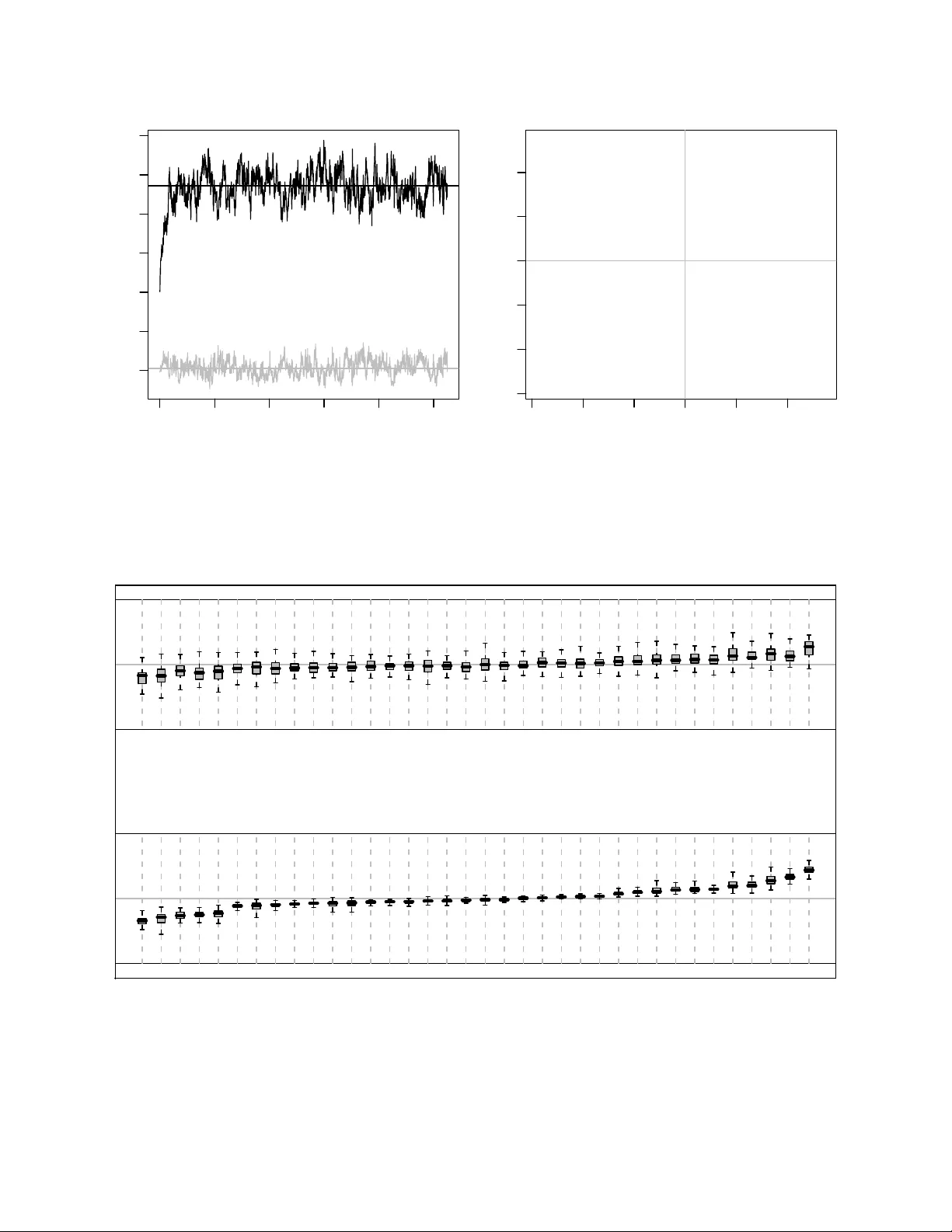
A hierarc hical eigenmo del for p o oled co v ariance estimation P eter D. Hoff ∗ Octob er 31, 2018 Abstract While a set of co v ariance matrices corresp onding to differen t p opulations are unlik ely to b e exactly equal they can still exhibit a high degree of similarity . F or example, some pairs of v ari- ables may be p ositiv ely correlated across most groups, while the correlation b et ween other pairs ma y be consisten tly negativ e. In suc h cases muc h of the similarity across co v ariance matrices can b e describ ed by similarities in their principal axes, the axes defined b y the eigenv ectors of the co v ariance matrices. Estimating the degree of across-p opulation eigen vector heterogeneity can b e helpful for a v ariet y of estimation tasks. Eigenv ector matrices can be p ooled to form a cen tral set of principal axes, and to the extent that the axes are similar, cov ariance estimates for p opu- lations having small sample sizes can b e stabilized b y shrinking their principal axes to wards the across-p opulation cen ter. T o this end, this article develops a hierarchical model and estimation pro cedure for p o oling principal axes across several p opulations. The mo del for the across-group heterogeneit y is based on a matrix-v alued antipo dally symmetric Bingham distribution that can flexibly describ e notions of “cen ter” and “spread” for a p opulation of orthonormal matrices. Some key wor ds : Ba yesian inference, copula, Marko v chain Monte Carlo, principal comp onen ts, random matrix, Stiefel manifold. 1 In tro duction Principal comp onen t analysis is a well-established pro cedure for describing the features of a co- v ariance matrix. Letting U Λ U T b e the eigen v alue decomp osition of the cov ariance matrix of a p -dimensional random vector y , the principal comp onen ts of y are the elements of the transformed mean-zero v ector U T ( y − E[ y ]). F rom the orthonormalit y of U it follows that the elements of the principal comp onen t vector are uncorrelated, with v ariances equal to the diagonal of Λ. P erhaps more importantly , the matrix U pro vides a natural co ordinate system for describing the orien tation ∗ Departmen ts of Statistics and Biostatistics, Universit y of W ashington, Seattle, W ashington 98195-4322. W eb: http://www.stat.washington.edu/hoff/ . This research was partially supported by NSF grant SES-0631531. The author thanks Mic hael Perlman for helpful discussions. 1 of the m ultiv ariate density of y : Letting u j denote the j th column of U , y can b e expressed as y − E[ y ] = z 1 u 1 + · · · + z p u p , where ( z 1 , . . . , z p ) T is a v ector of uncorrelated mean-zero random v ariables with diagonal cov ariance matrix Λ. Often the same set of v ariables are measured in multiple p opulations. Even if the co v ariance matrices differ across p opulations, it is natural to exp ect that they share some common structure, suc h as the correlations b et ween some pairs of v ariables having common signs across the p opulations. With this situation in mind, Flury [1984] developed estimation and testing procedures for the “common principal comp onen ts” model, in whic h a set of co v ariance matrices { Σ 1 , . . . , Σ K } ha ve common eigen vectors, so that Σ j = U Λ j U T for eac h j ∈ { 1 , . . . , K } . A n um b er of v ariations of this mo del hav e since app eared: Flury [1987] and Schott [1991, 1999] consider cases in which only certain columns or subspaces of U are shared across p opulations, and Boik [2002] describes a v ery general mo del in which eigenspaces can b e shared b et ween all or some of the p opulations. These approac hes all assume that certain eigenspaces are either exactly equal or completely distinct across a collection of co v ariances matrices. In many cases these t wo alternatives are to o extreme, and it ma y b e desirable to recognize situations in whic h eigen vectors are similar but not exactly equal. T o this end, this article develops a hierarc hical mo del to assess heterogeneity of principal axes across a set of p opulations. This is accomplished with the aid of a probabilit y distribution o ver the orthogonal group O p whic h can b e used in a hierarchical mo del for sample co v ariance matrices, allowing for p o oling of co v ariance information and a description of similarities and differences across p opulations. Sp ecifically , this article dev elops a sampling mo del for across- p opulation cov ariance heterogeneity in which p ( U | A , B , V ) = c ( A , B )etr( BU T VAV T U ) (1) U 1 , . . . , U K ∼ i.i.d. p ( U | A , B , V ) Σ k = U k Λ k U T k , where A and B are diagonal matrices and V ∈ O p . The ab o v e distribution is a t yp e of general- ized Bingham distribution [Khatri and Mardia, 1977, Gupta and Nagar, 2000] that is appropriate for mo deling principal comp onen t axes. Section 2 of this article describes some features of this distribution, in particular ho w A and B represen t the v ariability of { U 1 , . . . , U K } and ho w V represen ts the mo de. P arameter estimation is discussed in Section 3, in which a Marko v c hain Mon te Carlo algorithm is dev elop ed whic h allo ws for the joint estimation of { A , B , V } as well as { ( U k , Λ k ) , k = 1 , . . . , K } . The estimation sc heme is illustrated with tw o example data analyses in Sections 4 and 5. The first dataset, previously analyzed by Flury [1984] and Boik [2002] among others, in volv es skull measuremen t data on four p opulations of voles. Mo del diagnostics and com- parisons indicate that the prop osed hierarc hical model represents certain features of the observed co v ariance matrices b etter than do less flexible mo dels. The second example inv olv es surv ey data 2 from different states across the U.S.. The n umber of observ ations p er state v aries a great deal, and man y states hav e only a few observ ations. The example shows how the hierarchical mo del shrinks correlation estimates to wards the across-group cen ter when within-group data is limited. Section 6 pro vides a discussion of the hierarc hical mo del and a few of extensions of the approach. 2 A generalized Bingham distribution The eigenv alue decomp osition of a positive definite co v ariance matrix Σ is giv en by Σ = U Λ U T , where Λ is a diagonal matrix of positive n umbers ( λ 1 , . . . , λ p ) and U is an orthonormal matrix, so that U T U = UU T = I . W riting U Λ U T = P p j =1 λ j u j u T j , w e see that m ultiplication of a column of U b y -1 do es not change the v alue of the cov ariance matrix, highligh ting the fact that that the columns of U represent not directions of v ariation, but axes. As such, any probabilit y mo del represen ting v ariabilit y across a set of principal axes should b e antipo dally symmetric in the columns of U , meaning that U is equal in distribution to US for any diagonal matrix S having diagonal elemen ts equal to plus or min us one, since U and US represen t the same axes. Bingham [1974] describ ed a probability distribution ha ving a densit y prop ortional to exp { u T Gu } for normal vectors { u : u T u = 1 } . This densit y has antipo dal symmetry , making it a candidate mo del for a random axis. Khatri and Mardia [1977] and Gupta and Nagar [2000] discuss a matrix- v ariate version of the Bingham distribution, p ( U | G , H ) ∝ etr( HU T GU ) (2) where G and H are p × p symmetric matrices. Using the eigenv alue decomp ositions G = VAV T and H = WBW T , this densit y can b e rewritten as p ( U | A , B , V , W ) ∝ etr( B [ W T U T V ] A [ V T UW ]). A well-kno wn feature of this densit y is that it dep ends on A and B only through the differences among their diagonal elements. This is because for an y orthonormal matrix X (suc h as V T UW ), w e hav e tr([ B + d I ] X T [ A + c I ] X ) = tr( BX T AX ) + d × tr( X T AX ) + c × tr( BX T X ) + cd × tr( X T X ) = tr( BX T AX ) + d × tr( A ) + c × tr( B ) + cdp and so the probabilit y densities p ( U | A , B ) and p ( U | A + c I , B + d I ) are prop ortional as functions of U and therefore equal. By conv en tion A and B are usually taken to be non-negative. In what follo ws we will set the smallest eigen v alues a p and b p to b e equal to zero. Although a flexible class of distributions for orthonormal matrices, densities of the form (2) are not necessarily an tip odally symmetric. How ev er, we can identify conditions on G and H which giv e the desired symmetry . If either G or H hav e only one unique eigen v alue, then tr( HU T GU ) is constant in U and therefore trivially an tip o dally symmetric in the columns of U . Otherwise, we ha ve the following result: 3 Prop osition 1. If G and H b oth have mor e than one unique eigenvalue, then a ne c essary and sufficient c ondition for tr( HU T GU ) to b e antip o dal ly symmetric in the c olumns of U is that H b e a diagonal matrix. Pr o of. The symmetry condition requires that tr( HU T GU ) = tr( SHSU T GU ) for all U ∈ O p and diagonal sign matrices S . If H is diagonal then SHS = H and so diagonalit y is a sufficien t condition for an tip odal symmetry . T o show that it is also a necessary condition, first let V and A b e the eigen vector and eigenv alue matrices of G . Then for any orthonormal X w e hav e X = U T V if U = VX T . Therefore the symmetry condition is that tr([ H − SHS ] XAX T ) = 0 for all X ∈ O p and S ∈ { diag ( s ) , s ∈ {± 1 } p } . If we let diag( S ) = ( − 1 , 1 , 1 , . . . , 1) then D = H − SHS is zero except for p ossibly D [1 , − 1] and D [ − 1 , 1] , the first ro w and column of D absen t d 1 , 1 . Additionally , if not all en tries are zero then D is of rank tw o with eigen v ectors e and Se , where e = ( | H [ − 1 , 1] | , h 2 , 1 , h 3 , 1 , . . . , h p, 1 ) / ( √ 2 | H [ − 1 , 1] | ), and corresp onding eigenv alues ± d , where d = 2 | H [ − 1 , 1] | . W riting the symmetry condition in terms of the eigen v alues and vectors of D gives 0 = tr( DXAX T ) = d p X i =1 a i x T i  ee T − See T S  x i . The symmetry condition requires that this hold for all orthonormal X . No w if k and l are the indices of an y tw o unequal eigenv alues of G , we can let x k = e and x l = − Se , giving 0 = tr( DXAX T ) = d [ a k (1 − e T See T Se ) + a l ( e T See T Se − 1)] = d (1 − [ e T Se ] 2 )( a k − a l ) . Since a k 6 = a l b y assumption, this means that either d = 0 or ( e T Se ) 2 = 1. Neither of these conditions are met unless all entries of D are zero, implying that the off-diagonal elemen ts in the first row and column of H must b e zero. Rep eating this argument with the diagonal of S ranging o ver all p -vectors consisting of one negativ e-one and p − 1 p ositiv e ones shows that all off-diagonal elemen ts of H must b e zero. Based on this results w e fix the eigen vector matrix of H to b e I and our column-wise an tip o dally symmetric mo del for U ∈ O p is p B ( U | A , B , V ) = c ( A , B )etr( BU T VAV T U ) (3) where A and B are diagonal matrices with a 1 ≥ a 2 ≥ · · · ≥ a p = 0, b 1 ≥ b 2 ≥ · · · ≥ b p = 0 and V ∈ O p . In terpreting these parameters is made easier b y writing X = V T U and expanding out the exp onen t of p B as tr( BU T VAV T U ) = p X i =1 p X j =1 a i b j ( v T i u j ) 2 = p X i =1 p X j =1 a i b j x 2 i,j = a T ( X ◦ X ) b , (4) 4 where “ ◦ ” is the Hadamard pro duct denoting element-wise m ultiplication. The v alue of x 2 i,j de- scrib es how close column i of V is to column j of U . Since b oth a and b are in decreasing order, a 1 b 1 is the largest term and the density will b e large when x 2 1 , 1 is large. Ho wev er, due to the orthonormalit y of X , a large x 2 1 , 1 restricts x 2 1 , 2 and x 2 2 , 1 to b e small, whic h then allows x 2 2 , 2 to b e large. Con tinuing on this wa y suggests that the density is maximized if X ◦ X is the identit y , i.e. U = VS for some diagonal sign matrix S . Prop osition 2. The mo des of p B include V and { VS : S = diag ( s ) , s ∈ {± 1 } p } . If the diagonal elements of A and B ar e distinct then these ar e the only mo des. Pr o of. The matrix X ◦ X is an elemen t of the set of orthostochastic matrices, a subset of the doubly sto c hastic matrices. The set of doubly sto c hastic matrices is a compact conv ex set whose extreme p oin ts are the permutation matrices. Since ev ery element of this compact con v ex set can b e written as a con vex combination of the extreme p oin ts, w e hav e max X ∈O p a T ( X ◦ X ) b ≤ max θ a T ( X θ k P k ) b for probability distributions θ ov er the finite set of p erm utation matrices. If the elements of a and b are distinct and ordered it is easy to show that a T Pb is uniquely maximized ov er p ermutation matrices P by P = I , and so the right-hand side is maximized when θ is the point-mass measure on I . Since I is orthosto c hastic, the maximum on the left-hand side is achiev ed at ( X ◦ X ) = I . If tw o adjacen t eigen v alues are equal then the density has additional maxima. F or example, if b 1 = b 2 then a T Zb is maximized o ver doubly stochastic matrices Z b y an y con vex com bination of the matrices corresponding to the p erm utations { 1 , 2 , 3 , . . . , p } and { 2 , 1 , 3 , . . . , p } . In terms of U , this w ould mean that modes are suc h that u T i v i = ± 1 for i > 2, with u 1 and u 2 b eing an y orthonormal vectors in the n ull space of { v 3 , . . . , v p } . More generally , ho w the parameters ( A , B ) con trol the v ariabilit y of U around V can b e seen b y rewriting the exp onen t of (3) a few different w ays. F or example, equation (4), can b e expressed as tr( BU T VAV T U ) = p X i =1 p X j =1 a i b j ( v T i u j ) 2 = p X j =1 b j u T j ( VAV T ) u j (5) F rom equations (4) and (5) it is clear that b j = b j +1 implies that u j d = u j +1 and a i = a i +1 implies v T i u j d = v T i +1 u j . In this wa y the mo del can represen t eigensp ac es of high probabilit y , not only eigen vectors, providing a probabilistic analog to the common space models of Flury [1987]. T o illustrate this further, Figure 1 sho ws the exp ectations of the squared elemen ts of X = V T U for 5 1 2 3 4 5 6 column row 6 5 4 3 2 1 1 2 3 4 5 6 column 6 5 4 3 2 1 Figure 1: Exp ected v alues of the squared entries of X = V T U under t wo differen t Bingham distributions. Light shading indicates high v alues. t wo differen t v alues of ( A , B ) (calculations were based on a Monte Carlo appro ximation scheme describ ed in Hoff [2007b]). The plot in the first panel is based on the generalized Bingham distribu- tion in which diag( A ) = diag ( B ) = (7 , 5 , 3 , 0 , 0 , 0). F or this distribution, u 1 , u 2 and u 3 are highly concen trated around v 1 , v 2 and v 3 resp ectiv ely . Since b 4 = b 5 = b 6 , the v ectors u 4 , u 5 and u 6 are equal in distribution and close to b eing uniformly distributed on the null space of ( v 1 , v 2 , v 3 ). These particular v alues of ( A , B ) could represent a situation in whic h the first three eigen vectors are conserv ed across p opulations but the others are not. The second panel of Figure 1 represents a more complex situation in whic h diag ( A ) = (7 , 5 , 3 , 0 , 0 , 0) and diag( B ) = (7 , 7 , 0 , 0 , 0 , 0). F or these parameter v alues the following comp onen ts of X = V T U are equal in distribution: columns 1 and 2; columns 3, 4, 5 and 6; rows 2 and 3; ro ws 4, 5 and 6. Suc h a distribution migh t represent a situation in which a v ector v 1 is shared across p opulations, but it is equally likely to b e represen ted within a p opulation by either u 1 or u 2 . 3 P o oled estimation of cov ariance eigenstructure In the case of normally distributed data the sampling mo del for S k = Y T k ( I − 1 n k 11 T ) Y k , the observ ed sum of squares matrix in p opulation k , is a Wishart distribution. Com bining this with the mo del for principal axes dev elop ed in the last section gives the follo wing hierarchical mo del for co v ariance structure: U 1 , . . . , U K ∼ i . i . d . p ( U | A , B , V ) (across-p opulation v ariabilit y) S k ∼ Wishart( U k Λ k U T k , n k − 1) (within-population v ariabilit y) 6 The unkno wn parameters to estimate include { A , B , V } as w ell as the within-p opulation cov ariance matrices, parameterized as { ( U 1 , Λ 1 ) , . . . , ( U K , Λ K ) } . In this section w e describ e a Mark ov c hain Mon te Carlo algorithm that generates appro ximate samples from the posterior distribution for these parameters, allowing for estimation and inference. The Marko v c hain is constructed with Gibbs sampling, in whic h each parameter is iterativ ely resampled from its full conditional distributions. W e first describ e conditional up dates of the across-population parameters { A , B , V } , then describ e p ooled estimation of eac h U k , which com bines the p opulation-sp ecific information S k with the across-p opulation information in { A , B , V } . 3.1 Estimation of across-p opulation parameters Letting the prior distribution for V b e the uniform (in v arian t) measure on O p , w e hav e p ( V | A , B , U 1 , . . . , U K ) ∝ p ( V ) K Y k =1 p ( U k | A , B , V ) ∝ etr( K X k =1 BU T k VAV T U k ) = etr( K X k =1 AV T U k BU T k V ) = etr( AV T [ X U k BU T k ] V ) , and so the full conditional distribution of V is a generalized Bingham distribution, of the same form as describ ed in the previous section. Conditional on the v alues { A , B , U 1 , . . . , U K } , pairs of columns of V can b e sampled from their full conditional distributions using a metho d describ ed in Hoff [2007b]. Obtaining full conditional distributions for A and B is more complicated. The joint densit y of { U 1 , . . . , U K } is c ( A , B ) K etr( P AV T U k BU T k V ). F rom the terms in the exp onen t w e hav e tr( X BU T k V T AV T U k ) = K X k =1 tr( BU T k VAV T U k ) = K X k =1 p X i =1 p X j =1 a i b j ( v T i u j,k ) 2 = a T Mb where M is the matrix M = P K k =1 ( V T U k ) ◦ ( V T U k ). The normalizing constan t c ( A , B ) is equal to 0 F 0 ( A , B ) − 1 , where 0 F 0 ( A , B ) is a t yp e of h yp ergeometric function with matrix argumen ts [Herz, 1955]. Exact calculation of this quan tity is problematic, although approximations ha v e b een discussed in Anderson [1965], Constantine and Muirhead [1976] and Muirhead [1978]. The first-order term in these approximations is c ( A , B ) ≈ ˜ c ( A , B ) = 2 − p π − ( p 2 ) e − a T b Y i 0, p ( U | A , B , V ) = p ( U | c A , c − 1 B , V ), and so the scale of A and B are not separately identifiable. T o accoun t for this, we parameterize A and B as follo ws: diag( A ) = ( a 1 , . . . , a p ) = √ w ( α 1 , . . . , α p ) diag( B ) = ( b 1 , . . . , b p ) = √ w ( β 1 , . . . , β p ) where w > 0, 1 = α 1 > α 2 > · · · > α p − 1 > α p = 0 and 1 = β 1 > β 2 > · · · > β p − 1 > β p = 0. Rewriting (6) in terms of these parameters and multiplying by a prior distribution p ( α , β , w ) gives p ( α , β , w | M ) ∝ p ( α , β , w ) × exp {− w α T ( K I − M ) β } w ( p 2 ) K/ 2 Y i α 2 > · · · > α p − 1 > 0 and 1 > β 2 > · · · > β p − 1 > 0 are tw o indep enden t sets of order statistics of uniform random v ariables on [0 , 1], and w has a gamma distribution. With these priors, the v alues of α and β can b e sampled from their full conditional distributions on a grid of [0 , 1], and the full conditional distribution of w is a gamma distribution. F or example, if w ∼ gamma( η 0 / 2 , τ 2 0 / 2) a priori , then p ( w | α , β , M ) is gamma( η 0 / 2 +  p 2  K/ 2 , η 0 τ 2 0 / 2 + α T ( K I − M ) β ). W e should k eep in mind that this full conditional distribution is based on an approximation to the normalizing constant c ( A , B ) (although it is a “b ona fide” full conditional distribution under the prior ˜ p ( A , B ) = p ( A , B )[ ˜ c ( A , B ) /c ( A , B )] K ). Results from Anderson [1965] show that in terms of the parameters { α , β , w } , c ( A , B ) ˜ c ( A , B ) ≈ 1 + 1 4 w X i λ 2 ,k > · · · > λ p,k . The full conditional distribution of λ j,k is then in verse- gamma[( ν 0 + n − 1) / 2 , ( ν 0 σ 2 0 + u T j,k S k u j,k ) / 2] but restricted to the interv al ( λ j +1 ,k , λ j − 1 ,k ). 3.4 Summary of MCMC algorithm The unknown parameters in the hierarchical mo del are the group-sp ecific eigen vectors and v alues { U 1 , Λ 1 } , . . . , { U K , Λ K } and the parameters { A , B , V } describing the across-group heterogeneity of eigen vector matrices. The diagonal matrices A and B are parameterized as diag( A ) = ( a 1 , . . . , a p ) = √ w ( α 1 , . . . , α p ) diag( B ) = ( b 1 , . . . , b p ) = √ w ( β 1 , . . . , β p ) with 1 = α 1 > · · · > α p = 0 and 1 = β 1 > · · · > β p = 0. Conv enien t prior distributions are V ∼ uniform O p , ( α 2 , . . . , α p − 1 ) and ( β 2 , . . . , β p − 1 ) are uniform on [0 , 1] sub ject to the ordering restric- tion, w ∼ gamma( η 0 / 2 , τ 2 0 / 2) and (1 /λ 1 ,k , . . . , 1 /λ p,k ) are the order statistics of a sample from a gamma( ν 0 / 2 , σ 2 0 / 2) distribution. With these prior distributions, a Marko v chain in the unknown pa- rameters that con verges to the p osterior distribution p ( { U 1 , Λ 1 } , . . . , { U K , Λ K } , A , B , V | Y 1 , . . . , Y k ) can b e constructed by iteration of the follo wing sampling scheme: 1. Update the within-group parameters: (a) Update { U 1 , . . . , U K } : F or each k and a randomly selected pair { j 1 , j 2 } ⊂ { 1 , . . . , p } ; i. let N b e the n ull space of the columns { u j,k : j 6∈ { j 1 , j 2 }} ; ii. compute G = N T ( b j 1 VAV T − λ − 1 j 1 ,k S k ) N , H = N T ( b j 2 VAV T − λ − 1 j 2 ,k S k ) N ; iii. sample Z = ( z 1 , z 2 ) ∈ O 2 from the densit y prop ortional to exp( z T 1 Gz 1 + z T 2 Hz 2 ) iv. set u j 1 ,k to b e the first column of NZ and u j 2 ,k to b e the second. (b) Update { Λ 1 , . . . , Λ K } : Iterativ ely for eac h j ∈ { 1 , . . . , p } and k ∈ { 1 , . . . , K } , sample λ j,k ∼ in verse-gamma[( ν 0 + n k − 1) / 2 , ( ν 0 σ 2 0 + u T j,k S k u j,k ) / 2], but constrained to b e in ( λ j − 1 ,k , λ j +1 ,k ). 2. Update the across-group parameters: (a) Update V : Sample V from the Bingham densit y prop ortional to etr( AV T [ P U k BU T k ] V ). (b) Update w , α and β : Compute M = P K k =1 ( V T U k ) ◦ ( V T U k ) and 11 i. sample w ∼ gamma( η 0 / 2 +  p 2  K/ 2 , η 0 τ 2 0 / 2 + α T [ K I − M ] β ) ii. for each i ∈ { 2 , . . . , p − 1 } sample α i ∈ ( α i − 1 , α i +1 ) from the density prop ortional to exp {− α i ( w β T M [ i, ] ) } Q j : j 6 = i | a i − a j | K/ 2 . iii. for eac h j ∈ { 2 , . . . , p − 1 } sample β j ∈ ( β j − 1 , β j +1 ) from the density prop ortional to exp {− β j ( w M T [ ,j ] α ) } Q i : i 6 = j | β j − β i | K/ 2 . As discussed in section 3.1, it may b e desirable to make Metrop olis-Hastings adjustments to the steps in 2(b) to accoun t for the approximation to the normalizing constant c ( A , B ). F unctions and example co de for this algorithm, written in the R programming environmen t, are a v ailable at m y w ebsite, http://www.stat.washington.edu/hoff/ . 4 Example: V ole measuremen ts Flury [1987] describ es an analysis of skull measurements on four different groups of voles. The four groups, defined b y sp ecies and sex, are male and female Micr otus c alifornicus and male and female Micr otus o chr o gaster , ha ving sample s izes of 82, 70, 58 and 54 resp ectiv ely . Flury provides the sample cov ariance matrices of four log-transformed measuremen ts corresp onding to skull length, to othro w length, c heekb one width and interorbital width. The eigenv ectors of the four empirical co v ariance matrices are given in T able 1. The first eigenv ector in each group can roughly b e in terpreted as measuring ov erall size v ariation, and its v alues seem fairly similar across groups. The remaining eigen vectors also display a high degree of similarit y across groups. By p erforming statistical tests of v arious h yp otheses regarding the four p opulation cov ariance matrices, Flury concludes that although the sample co v ariance matrices app ear similar, there is enough evidence to reject exact equality of the p opulation matrices. F urthermore, Flury rejects a hypotheses that the p opulation co v ariances are prop ortional to eac h other, and then suggests a mo del in which the the co v ariance matrices share a single eigenv ector (in terpreted as corresp onding to size), with the remaining eigenv ectors and all of the eigen v alues b eing distinct across groups. In this section w e reanalyze these data using the hierarchical eigenmodel discussed ab ov e, and compare it to the mo del in Flury [1987] and a few others. In particular, w e sho w that allowing information-sharing across the groups where appropriate, but not forcing any of the eigen v ectors to b e exactly equal, results in a model that b etter represen ts features of the observed dataset. Using the sample sizes and sample co v ariance matrices provided in Flury [1987], cen tered ver- sions of Y T k Y k for each group k ∈ { 1 , . . . , 4 } w ere reconstructed and used as data for the mo del describ ed in Section 3. The prior distribution of w w as tak en to b e a diffuse exp onen tial with a mean of 1000, and the prior distribution for the in verse-eigen v alues was exp onential with a mean of 1. A Mark ov chain consisting of 10,000 iterations was constructed, for whic h parameter v alues w ere sav ed every 10th iteration giving a total of 1000 p osterior samples for each parameter. Mixing 12 M. c alifornicus males females 36.31 27.01 8.05 2.78 52.44 21.14 3.75 3.17 0.49 -0.31 -0.19 0.79 0.53 -0.31 -0.29 0.74 0.60 -0.10 0.76 -0.24 0.56 -0.06 0.82 -0.11 0.55 -0.12 -0.63 -0.54 0.57 -0.14 -0.48 -0.65 0.30 0.94 -0.06 0.17 0.30 0.94 -0.11 0.14 M. o chr o gaster males females 36.30 9.67 7.97 2.80 35.61 12.35 8.32 3.38 0.58 0.04 -0.38 0.71 0.56 0.06 0.05 0.82 0.45 0.72 0.51 -0.13 0.47 0.02 0.80 -0.38 0.51 -0.08 -0.51 -0.69 0.66 -0.25 -0.58 -0.40 0.45 -0.68 0.58 -0.02 0.13 0.97 -0.17 -0.14 T able 1: Eigenv alues and eigenv ectors of empirical cov ariance matrices. Eigenv alues are given in the first ro w for each group. of the Marko v c hains was monitored via a v ariet y of parameter summaries computed at each sav ed iteration. F or example, for eac h sav ed v alue of A and B the av erage and standard deviation of the logs of the ( p − 1) × ( p − 1) = 9 non-zero v alues of A ◦ B w ere obtained and plotted sequen tially in the first panel of Figure 2. A p osterior p oint estimate of V can b e obtained from the eigen vector matrix of the p osterior mean of VAV T , obtained b y av eraging across samples of the Marko v chain. This produces the matrix in T able 2, whic h is nearly iden tical to the eigenv ector matrix of the p o oled co v ariance matrix P Y T k Y k / ( n k − 1), which is also given in the table. Posterior mean estimates of the eigenv alue matrices { Λ 1 , . . . , Λ K } were all within 1.0 of their corresp onding v alues based on the the empirical co v ariance matrices. T able 1 suggests that the first and fourth eigen vectors are the most preserv ed across groups, whereas the other t wo are less well-preserv ed. Letting ˆ U k b e the eigen vector matrix of Y T k Y k and ˆ V the eigen vector matrix of P Y T k Y k / ( n k − 1), the differential heterogeneit y of the eigen vectors can b e describ ed numerically b y computing the v alue of diag ( ˆ V T ˆ U k ) 2 and av eraging each of the p en tries of this vector across the K groups. This p -dimensional function of the observed data giv es t ( Y T 1 Y 1 , . . . , Y T 4 Y 4 ) = (0 . 98 , 0 . 85 , 0 . 86 , 0 . 96), indicating that b y this metric the first and last eigenv ectors are most preserved across groups. T o examine how well the mo del represen ts this 13 hierarc hical mo del estimate empirical estimate 0.54 -0.27 -0.19 0.77 0.55 -0.25 -0.17 0.78 0.54 -0.10 0.80 -0.22 0.53 -0.10 0.81 -0.23 0.56 -0.15 -0.56 -0.59 0.57 -0.16 -0.56 -0.57 0.30 0.95 -0.06 0.10 0.30 0.95 -0.05 0.08 T able 2: Mo del-based and empirical estimates of V . observ ed heterogeneit y , the v alue of t ( Y T 1 Y 1 , . . . , Y T 4 Y 4 ) can b e compared to its posterior predictive distribution under the mo del. This was done b y generating simulated v alues ˜ Y 1 T ˜ Y 1 , . . . , ˜ Y T 4 ˜ Y 4 ev ery 10th iteration of the Mark ov chain and computing the statistic t () describ ed ab o v e, resulting in 1000 samples of t ( ˜ Y 1 T ˜ Y 1 , . . . , ˜ Y T 4 ˜ Y 4 ) from the p osterior predictiv e distribution. F or simplicity w e present b elo w only the minimum and maximum v alues of this statistic, whic h for our observed data are (0.85, 0.98). The top of the second panel of Figure 2 shows the p osterior predictive distributions of this statistic on a logit scale under the hierarchical model whic h p o ols information across eigen vector matrices. The observ ed v alues are well within the predicted range, indicating that the mo del is able to represen t the differen tial amounts of eigen v ector preserv ation among the observed cov ariance matrices. In contrast, the low er part of the plot shows a p osterior predictive distribution generated under a one-shared-eigen vector mo del similar to the one in Flury [1987], obtained obtained b y fixing w = 1000, α 1 = β 1 = 1 and α j = β j = 0 for j > 1. This mo del accurately predicts the highest degree of preserv ation across eigen vectors, but underestimates the preserv ation among other eigenv ectors. This is not surprising, as this mo del shares information only across a single eigen vector. Lastly we fit t wo other related models: a “no p ooling” model in which no information w as shared across groups and a common co v ariance matrix mo del in which it is assumed that the co v ariances are exactly iden tical across groups. Not surprisingly these tw o mo dels under- and ov er-represent the similarity across eigenv ectors of observed co v ariance matrices, as shown in the third panel of Figure 2. T aken together, these results indicate that assuming complete equalit y , or completely ignoring similarit y , can misrepresent the v ariabilit y of co v ariance structure across groups. 5 Example: National Health Comm unication Study The 2005 Annen b erg National Health Communication Surv ey ( anhcs.asc.upenn.edu ) gathered self-rep orted health and lifest yle data from 2,989 members of the adult U.S. population under the age of 65. Among the v ariables recorded were the following: 14 0 2000 4000 6000 8000 0 2 4 6 8 iteration −2 0 2 4 6 log t/(1 − − t) one shared vector hierarchical −2 0 2 4 6 log t/(1 − − t) no pooling common covariance matrix Figure 2: MCMC and model diagnostics for the V ole example. The first panel shows av erages (blac k) and standard deviations (gray) of the log entries of A ◦ B at every 10th scan of the Marko v c hain. The second and third panels sho w p osterior predictiv e distributions of the minim um and maxim um similarit y statistics under a v ariet y of mo dels, with the observ ed v alue of each statistic represen ted by a vertical line. state : state of residency (including the District of Columbia) fruitveg : t ypical num b er of servings of fruit and v egetables p er da y exercise : t ypical weekly frequency of exercise bmi : b ody mass index alcohol : n umber of days in the mon th consuming five or more alcoholic drinks smoke : t ypical num b er of cigarettes smoked p er day age : in y ears female : indicator of b eing female income : household income (19 ordered categories) edu : education lev el (no degree, high sc ho ol, some college, Bac helor’s degree or higher) In this section we estimate state-sp ecific correlation matrices in a Gaussian copula mo del for the p = 9 ordinal v ariables ab ov e. More sp ecifically , we mo del the observed data v ectors y 1 , . . . , y n within a particular state as monotone functions of latent Gaussian random v ariables, so that z 1 , . . . , z n ∼ i.i.d. multiv ariate normal( 0 , Σ) y i,j = g j ( z i,j ) . 15 The non-decreasing functions { g 1 , . . . , g p } are state-specific as is the cov ariance matrix Σ. W e compare tw o mo dels for Σ 1 , . . . , Σ K , the first b eing one in whic h no information is shared and U 1 , . . . , U K are a priori indep enden t and uniformly distributed on O p . The second is the hierar- c hical eigenmo del in whic h U 1 , . . . , U K ∼ i.i.d. p B ( U | A , B , V ), with the parameters { A , B , V } unkno wn and estimated from the data, using the same prior distributions as in the previous section. F or b oth models, the prior distribution on the eigenv alues in each group is such that { 1 /λ 1 < · · · < 1 /λ p } are the order statistics of p indep enden t exp onential(1) random v ariables. W e note that b oth of these mo dels ignore the p ossibility that heterogeneity in correlation matrices migh t be asso ciated with state-specific c haracteristics suc h as population size or geographic lo cation (although some ad-ho c exploratory analyses suggest these effects are small). P arameter estimation for this hierarc hical copula mo del can b e accomplished b y iterativ e sam- pling of the parameters from their full conditional distributions as in Section 3 with the laten t z ’s taking the roles of the observed y ’s, along with iterativ e sampling of the z ’s from their full conditional distributions (which are constrained normal distributions). This latter step is de- scrib ed for a one-group discrete-data copula mo del in Hoff [2007a]. W e note that this is a t yp e of parameter-expanded estimation sc heme [Gelman et al., 2008] in that the scale of eac h v ariable j can b e represented b y both g j and Σ j,j , and so these quan tities are not separately iden tifiable. Ho wev er, the p osterior distribution of { Σ 1 , . . . , Σ K } induces a posterior distribution o v er state- sp ecific correlation matrices { C 1 , . . . , C K } , which are the parameters of primary interest in copula mo dels. In the p osterior analysis that follows we fo cus mostly on comparing the hierarchical and non-hierarc hical p osterior mean estimates of the state-sp ecific correlation matrices. Mark ov chains consisting of 105,000 iterations were constructed for each of the tw o mo dels, with results from the first 5000 iterations being discarded to allow for burn-in. Parameter v alues from the remaining iterations w ere sav ed ev ery 50th iteration, leaving 2000 Mon te Carlo samples for appro ximating the p osterior distributions. The correlation parameters mixed reasonably well: In the hierarc hical mo del, the effective sample sizes for 90% of the parameters was greater than 500, and for 50% it w as greater than 1200 (effective sample size is an estimate of the n umber of indep enden t samples required to estimate the mean to the same precision as with a giv en auto- correlated sample). Mixing of the hierarc hical parameters was slow er: The first panel of Figure 5 plots the mean and standard deviation of the logs of the 64 non-zero v alues of the matrix A ◦ B at ev ery 50th scan of the Marko v chain for the hierarchical model. The effective sample sizes for these t wo functions of the parameters w ere b oth just o ver 100. The second panel of Figure 5 plots the first tw o eigenv ectors of the p osterior mean of the state- a veraged correlation matrix P K k =1 C k /K for each of the tw o mo dels. The results are quite similar, indicating that the main correlations across states are describ ed by smoking and drinking b eha vior b eing negativ ely correlated with education lev el, income, fruit and v egetable in take and exercise. In 16 0e+00 2e+04 4e+04 6e+04 8e+04 1e+05 1 2 3 4 5 6 7 iteration −0.6 −0.4 −0.2 0.0 0.2 0.4 −0.6 −0.4 −0.2 0.0 0.2 0.4 first principal component loadings second principal component loadings female fruitveg exercise bmi alcohol smoke age income edu female fruitveg exercise bmi alcohol smoke age income edu Figure 3: The first panel sho ws a v erages (blac k) and standard deviations (gray) of the log en tries of A ◦ B . The second panel sho ws the first tw o principal comp onen t loadings for the hierarchical (blac k) and non-hierarchical (gray) mo dels. ● ● ● ● ● ● ● ● ● ● ● ● ● ● ● ● ● ● ● ● ● ● ● ● ● ● ● ● ● ● ● ● ● ● ● ● ● ● ● ● ● ● ● ● ● ● ● ● ● ● ● ● ● ● ● ● ● ● ● ● ● ● ● ● ● ● ● ● ● ● ● ● ● ● ● ● ● ● ● ● ● ● ● ● ● ● ● ● ● ● ● ● ● ● ● ● ● ● ● ● ● ● ● ● ● ● ● ● ● ● ● ● ● ● ● ● ● ● ● ● ● ● ● ● ● ● ● ● ● ● ● ● ● ● ● ● ● ● ● ● ● ● ● ● ● ● ● ● ● ● ● ● ● ● ● ● ● ● ● ● ● ● ● ● ● ● ● ● smoke.edu exercise.smoke female.alcohol smoke.income fruitveg.smoke exercise.bmi fruitveg.alcohol bmi.edu alcohol.age bmi.income exercise.alcohol alcohol.edu female.income female.bmi fruitveg.bmi bmi.smoke bmi.alcohol female.smoke alcohol.income exercise.age smoke.age female.exercise fruitveg.age female.age age.edu female.edu age.income exercise.income fruitveg.income female.fruitveg bmi.age exercise.edu fruitveg.edu fruitveg.exercise alcohol.smoke income.edu Figure 4: Posterior mean estimates of state-sp ecific correlations. The top row are from the non- hierarc hical mo del, the bottom from the hierarchical eigenmo del. 17 terms of state-sp ecific correlation matrices how ev er, the tw o mo dels pro duce quite different results: The top and b ottom plots of Figure 5 give p osterior mean estimates of state-sp ecific correlations from the non-hierarchical and hierarc hical mo dels, respectively . F or eac h pair of v ariables, a b o xplot indicates the across-state heterogeneit y among the K = 51 parameter estimates for eac h correlation co efficien t. The n um b er of observ ations per state v aries widely , with North Dakota and the District of Colum bia ha ving 3 respondents each, whereas T exas and California hav e 225 and 312 respondents resp ectiv ely . Generally sp eaking, the estimates for states with lo wer sample sizes app ear at the extremes of the boxplots, whic h is not surprising as these estimates ha ve a higher degree of sampling v ariabilit y . Also of note is the fact that there is no co efficien t that is estimated as either p ositiv e across all states or negativ e across all states. F or example, among the highest correlations is that b et w een income and education, with an across-state median estimate of 0.28 based on the non- hierarc hical mo del. Ho wev er, there w ere four states (VT, AK, WY, NE) whic h w ere estimated as ha ving a negativ e correlation b et ween these v ariables. The sample sizes from these states w ere 5, 9, 5 and 15 resp ectiv ely , suggesting that these low correlations ma y b e due to unrepresentativ e samples. In contrast, the hierarchical mo del recognizes that muc h of the across-state heterogeneity in correlation estimates may b e due to sampling v ariabilit y , and shrinks estimates from low-sample size states tow ards the across-state center. F or example, the hierarchical mo del giv es p ositive point estimates for the correlation b etw een income and education for all of the states, including VT, AK, WY and NE. As shown in the low er half of Figure 5, across-state heterogeneit y among the other correlation co efficien ts is similarly reduced, with nearly t wo-thirds (23 of 36) of the correlation co efficien ts ha ving sign-consistent estimates across all 51 states. The effects of hierarchical estimation are explored further in Figure 5. W e hav e tw o estimates of the eigen vectors for each of the k state-sp ecific correlation matrices: ˆ U k from the hierarc hical mo del and ˇ U k from the non-hierarchical model. W e can compute a similarity b et ween these t wo matrices as the a verage of the p v alues of diag( ˇ U T k ˆ U k ) 2 . The first panel of Figure 5 shows that the relationship b et ween the similarit y and the within-state sample size is p ositiv e as exp ected: Co v ariance matrices for states with large sample sizes are well-estimated based on within-state data alone, and their eigen vector estimates are largely unaffected b y hierarchical estimation. In con trast, the amount of information from states with lo w sample sizes is small, and so the estimates for the hierarc hical mo del are pulled to wards the population mode and aw ay from ˇ U k . The effects of this shrink age on the principal axes of the correlation matrices are shown graphically in the second and third panels of Figure 5. The second panel plots the pro jections of the first t wo columns of eac h ˇ U k on to the first tw o columns of the eigenv ector matrix of the p o oled correlation matrix. Although heterogeneous, the vectors are generally in the same direction, and further insp ection shows that outliers tend to b e states with low sample sizes. The third panel of the figure shows the same plot for the pro jections of the columns of each ˆ U k from the hierarc hical mo del. The heterogeneit y here 18 ● ● ● ● ● ● ● ● ● ● ● ● ● ● ● ● ● ● ● ● ● ● ● ● ● ● ● ● ● ● ● ● ● ● ● ● ● ● ● ● ● ● ● ● ● ● ● ● ● ● ● 0 50 150 250 0.2 0.4 0.6 0.8 sample size eigenvector similarity first principal component second principal component first principal component second principal component Figure 5: Effects of shrink age on the estimated principal axes. The first panel sho ws the similarity b et w een non-hierarc hical and hierarc hical estimates as a function of sample size. The second and third show heterogeneity across the first tw o principal axes in the non-hierarchical and hierarchical mo dels, resp ectiv ely . represen ts the estimated across-state v ariabilit y in eigen vectors after accoun ting for the within- state sampling v ariabilit y . The axis in this plot that is furthest from the center is that representing Wisconsin, which has relativ ely high sample size of 69 but some extreme correlations: F or example, among states with sample sizes greater than 20, Wisconsin has the low est non-hierarc hical estimate of the correlation for ( income , education ) and ( female , bmi ), and the highest non-hierarchical estimate of the correlation for ( income , alcohol ). These correlations mak e Wisconsin somewhat of an outlier in terms of the correlations represen ted b y the first tw o principal components. The relativ ely large sample size for Wisconsin suggests these extreme correlations cannot b e solely attributed to within-state sampling v ariability , and this is reflected in the state-sp ecific estimated correlation matrix from the hierarchical mo del. 6 Discussion As an alternative to the Bingham distribution, a simpler mo del for across-group cov ariance hetero- geneit y w ould b e that Σ 1 , . . . , Σ K are i.i.d. samples from an in verse-Wishart distribution. F or many applications ho wev er, suc h a mo del ma y b e to o simple: The inv erse-Wishart distribution has only one parameter to represent heterogeneit y around the mean co v ariance matrix, and cannot represen t differen tial amounts of eigenv ector heterogeneity as the Bingham distribution can. Additionally , the in verse-Wishart mo del cannot distinguish b et ween across-group eigenv ector heterogeneity and across-group eigen v alue heterogeneit y , as these quan tities are mo deled sim ultaneously . As w e are p o oling eigenv ector information across groups it is natural to consider p o oling eigen- 19 v alues as well. This would entail mo deling { Λ 1 , . . . , Λ K } as being samples from a common p opu- lation, and estimating the parameters of this p opulation using the data from all K groups. One simple approac h to doing this w ould b e to estimate the parameters ( ν 0 , σ 2 0 ) in the prior distribu- tion for the eigen v alues, thus treating the distribution as a sampling mo del. As with the other unkno wn parameters, this can b e done by iteratively up dating these parameters based on their full conditional distributions. Straigh tforward calculations sho w that a gamma prior distribution for σ 2 0 results in a gamma full conditional distribution. The full conditional distribution for ν 0 is non-standard, but if ν 0 is restricted to the integers then its full conditional distribution can easily b e sampled from. Another p ossible mo del extension is to situations where the num b er of v ariables is larger than an y of the within-group sample sizes. In these cases, full-rank cov ariance estimation can b ecome unstable and computationally intractable. A remedy to this problem is to use a factor analysis mo del, in which a co v ariance matrix Σ k is assumed equal to U k D k U T k + σ 2 k I , where D k is a p ositiv e diagonal matrix and U k is a p × r orthonormal matrix with r < p , an elemen t of the Stiefel manifold S r,p . As b efore, heterogeneit y across co v ariance matrices can b e expressed b y heterogeneit y in these matrix comp onen ts, and a Bingham mo del on S r,p , similar to the one used in this pap er, can b e used to express heterogeneit y among U 1 , . . . , U K . Computer co de and data for the examples in this article are av ailable at http://www.stat.washington.edu/hoff/ . References George A. Anderson. An asymptotic expansion for the distribution of the laten t ro ots of the estimated co v ariance matrix. Ann. Math. Statist. , 36:1153–1173, 1965. ISSN 0003-4851. Christopher Bingham. An an tip o dally symmetric distribution on the sphere. Ann. Statist. , 2: 1201–1225, 1974. ISSN 0090-5364. Rob ert J. Boik. Sp ectral mo dels for co v ariance matrices. Biometrika , 89(1):159–182, 2002. ISSN 0006-3444. A. G. Constan tine and R. J. Muirhead. Asymptotic expansions for distributions of latent ro ots in m ultiv ariate analysis. J. Multivariate Anal. , 6(3):369–391, 1976. ISSN 0047-259x. Bernhard K. Flury . Tw o generalizations of the common principal comp onen t mo del. Biometrika , 74(1):59–69, 1987. ISSN 0006-3444. Bernhard N. Flury . Common principal comp onents in k groups. J. A mer. Statist. Asso c. , 79(388): 892–898, 1984. ISSN 0162-1459. 20 Andrew Gelman, Da vid A. v an Dyk, Zaiying Huang, and John W. Boscardin. Using redundan t parameterizations to fit hierarc hical mo dels. Journal of Computational and Gr aphic al Statistics , 17(1):95–122, Marc h 2008. A. K. Gupta and D. K. Nagar. Matrix variate distributions , volume 104 of Chapman & Hal l/CRC Mono gr aphs and Surveys in Pur e and Applie d Mathematics . Chapman & Hall/CRC, Bo ca Raton, FL, 2000. ISBN 1-58488-046-5. Carl S. Herz. Bessel functions of matrix argumen t. Ann. of Math. (2) , 61:474–523, 1955. ISSN 0003-486X. P eter D. Hoff. Extending the rank likelihoo d for semiparametric copula estimation. Ann. Appl. Statist. , 1(1):265–283, 2007a. P eter D. Hoff. Simulation of the matrix Bingham-von Mises-Fisher distribution, with applications to m ultiv ariate and relational data. T ec hnical rep ort, Universit y of W ashington, 2007b. C. G. Khatri and K. V. Mardia. The von Mises-Fisher matrix distribution in orien tation statistics. J. R oy. Statist. So c. Ser. B , 39(1):95–106, 1977. ISSN 0035-9246. Plamen Ko ev and Alan Edelman. The efficient ev aluation of the h yp ergeometric function of a matrix argumen t. Math. Comp. , 75(254):833–846 (electronic), 2006. ISSN 0025-5718. Robb J. Muirhead. Laten t ro ots and matrix v ariates: a review of some asymptotic results. Ann. Statist. , 6(1):5–33, 1978. ISSN 0090-5364. James R. Sc hott. Some tests for common principal comp onen t subspaces in sev eral groups. Biometrika , 78(4):771–777, 1991. ISSN 0006-3444. James R. Schott. Partial common principal comp onent subspaces. Biometrika , 86(4):899–908, 1999. ISSN 0006-3444. 21