Multisource Bayesian sequential change detection

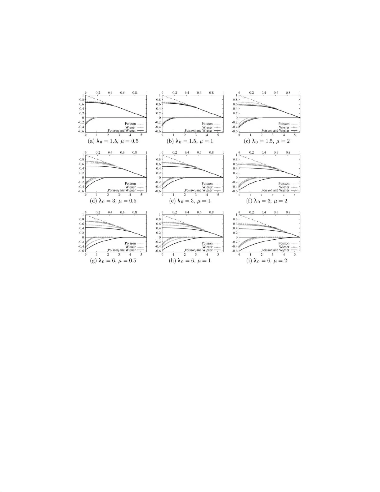
The Annals of Applie d Pr obabil ity 2008, V ol. 18, N o. 2, 552– 590 DOI: 10.1214 /07-AAP463 c  Institute of Mathematical Statistics , 2008 MUL TISOUR C E BA YESIA N SEQUENTIAL C HANGE DE TE CTION By Sa v as D a y anik, 1 H. Vincent Poor 2 and Semih O. Sezer 2 Princ eton University , Princ eton University and University of Michigan Supp ose that local chara cteristics of several indep en dent com- p ound P oisson and Wiener processes change suddenly and sim u lta- neously at some unobserv able d isorder time. The problem is to detect the disorder time as qu ic kly as p ossible after it h app ens and minimize the rate of false alarms at the same time. These problems arise, for example, from managing pro duct quality in manufacturing systems and preventi ng the spread of infectious diseases. The p romptness and accuracy of detection rules improv e greatly if multiple indep end ent information sources a re a vai lable. Earl ier w ork on sequential change detection in continuous time do es not pro vide optimal rules for situa- tions in which several marked count data and contin uously changing signals are sim u ltaneously observ able. In t his pap er, optimal Ba yesian sequential d etection rules are d evelo p ed for such problems when the marked count data is in the form of indep endent comp ound Pois- son p ro cesses, and the contin uously changing signals form a multi- dimensional Wiener process. An auxiliary opt imal stopping problem for a jump - diffusion pro cess is solved by transforming it first into a sequence of optimal stopping p roblems for a pure diffu sion by means of a jump op erator. This meth o d is n ew and can b e very useful in other applications as we ll, b ecause it allow s the use of t he p ow erful optimal stopp ing theory fo r diffu sions. 1. Introdu ction. Supp ose t hat at some unobserv able disorder time Θ, the lo cal c haracteristics of several indep end en t comp oun d P oisson and Wiener pro cesses undergo a sudd en and sim u ltaneous c hange. More precisel y , the Received Novem b er 2006; revised July 2007. 1 Supp orted in p art by the Air F orce Office of S cientific Resea rc h, Gran t AFOSR- F A9550 -06-1-0496, and by the U.S. Department of H omeland Security through the Center for Dynamic Data Analysis f or Homeland Security admin istered through O N R Grant N00014-07-1-0150 to Rutgers Universit y . 2 Supp orted by the U.S. Arm y P antheon Program. AMS 2000 subje ct classific ations. Primary 62L10; secondary 62L15, 62C10, 60G40. Key wor ds and phr ases. Seq u ential change detection, jump-diffusion pro cesses, optimal stopping. This is an electronic reprint of the original article published b y the Institute of Mathematical Statistics in The Annals of Applie d Pr ob ability , 2008, V ol. 18, No. 2, 552–59 0 . This reprint differs fr om the original in pagination and t yp og raphic detail. 1 2 S. DA Y ANI K, H. V. POOR AND S. O. SEZER pairs ( λ ( i ) 0 , ν ( i ) 0 ), 1 ≤ i ≤ m , consisting of t he arriv al rate and mark distri- bution of m comp ound P oisson pr o cesses ( T ( i ) n , Z ( i ) n ) n ≥ 1 , 1 ≤ i ≤ m , b ecome ( λ ( i ) 1 , ν ( i ) 1 ), 1 ≤ i ≤ m , and d Wiener pro cesses W ( j ) t , 1 ≤ j ≤ d gain drifts µ ( j ) , 1 ≤ j ≤ d at time Θ . W e assum e that Θ is a r an d om v ariable with the zero-mo dified exp onential distribution P { Θ = 0 } = π and P { Θ > t } = (1 − π ) e − λt , t ≥ 0 , (1.1) and ( λ ( i ) 0 , ν ( i ) 0 ) 1 ≤ i ≤ m , ( λ ( i ) 1 , ν ( i ) 1 ) 1 ≤ i ≤ m , ( µ ( j ) ) 1 ≤ j ≤ d , π , and λ are kno wn. Th e ob jectiv e is to d etect the disorder time Θ as so on as p ossible after d isorder happ en s by using the ob s erv ations of ( T ( i ) n , Z ( i ) n ) n ≥ 1 , 1 ≤ i ≤ m , and X ( j ) t = X ( j ) 0 + µ ( j ) ( t − Θ ) + + W ( j ) t , t ≥ 0 , 1 ≤ j ≤ d. More precisely , if F = {F t } t ≥ 0 denotes the observ ation fi ltration, then w e w ould lik e to find , if it exists, an F -stopping time τ w h ose Ba y es risk R τ ( π ) , P { τ < Θ } + c E ( τ − Θ ) + , 0 ≤ π < 1 (1.2) is the smallest f or an y giv en constan t cost parameter c > 0 and calculate its Ba y es risk . If suc h a stopping time exists, then it provides the b est trade-off b et w een false alarm frequency P { τ < Θ } and exp ected detection d ela y cost c E ( τ − Θ ) + . Imp ortant applications of this problem are the quick est detecti on of man- ufacturing defects during p ro du ct qualit y assurance, online fault d etectio n and iden tification f or cond ition-based equipmen t main tenance, p rompt de- tection of shifts in the riskiness of v arious financial instruments, early detec- tion of the onset of an epidemic to pr otect pub lic health, quic k est detection of a threat to homeland securit y , and online detection of u nauthorized access to pr ivileged r esources in the fi gh t against fraud . In many of those applica- tions, a range of data, c hanging o v er time either co n tinuously or by jumps or b oth, are collected from multiple sources/sensors in order to d etect a su dden unobserved c hange as quickly as p ossible after it happ ens, and the problems can b e mo deled as the quic kest detection of a c hange in the lo cal characte r - istics of sev eral Wiener and comp ound P oisson pro cesses. F o r example, in condition-based m aintenance, an equipment is monitored con tinuously by a w eb of sensors for b oth con tinuously-c hanging data (suc h as oil leve l, tem- p erature, pressure) an d mark ed count data (e.g., num b er, size and t yp e of w ear particles in the oil); see Byington and Garga [ 6 ]. F or the assessmen t of financial risks of an elect ricit y d eliv ery cont ract, the sp ot price of electricit y is sometimes mo deled by a jump -d iffusion p ro cess; see, for example, W eron, Bierbrauer and T r ¨ uc k [ 18 ] and Cartea and Figueroa [ 7 ]. In the past, the Ba ye sian sequen tial c hange-detection problems ha v e b een studied for Wiener pr o cesses by S hirya ev [ 17 , Chapter 4 ] a nd for Poisson MUL TIS OURCE BA YESIAN SEQUENTIA L CHAN GE DETECTION 3 pro cesses by P eskir and Sh iry aev [ 14 , 15 ], Gap eev [ 10 ], Ba yraktar, Da y anik and Karatzas [ 2 , 3 ] a nd Da y anik and Sezer [ 9 ], b ut ha v e n ev er b een con- sidered for the combination of Wiener and P oisson pro cesses. Clearly , an unobserved c hange can b e detected more accurately if there are multi ple indep en d en t sources of inform ation ab out the disorder time. If all of the information sour ces consist of exclusiv ely either Wiener or P oisson p ro cess observ ations, then the problem can b e solv ed b y applying th e r esults of Shiryae v ([ 17 ], Chapter 4) in the Wiener case and Da y anik and Sezer [ 9 ] in the Poisson case to a w eigh ted linear com bination or su p erp osition of all observ ation pr o cesses; see Section 5 . If Wiener and Po iss on pro cesses can b e observ ed simultaneously , then previous w ork do es not pro vide an answer; the solution of the p roblem in this case is the curr en t pap er’s con trib ution. W e solv e the problem in detail for m = d = 1 , namely , when we observe exactly one Wiener an d one P oisson pro cess simulta neously; in S ection 5 w e sho w th e easy exte nsion t o multiple Wiener and multiple Po iss on p ro- cesses. Therefore, except in S ection 5 , we drop all of the sup erscripts in th e sequel. W e sho w that the first time τ [ φ ∞ , ∞ ) , inf { t ≥ 0; Φ t ≥ φ ∞ } that the conditional o dd s-ratio pro cess Φ t , P { Θ ≤ t | F t } P { Θ > t | F t } , t ≥ 0 (1.3) en ters into some half-line [ φ ∞ , ∞ ) ⊂ R + giv es the smallest Ba y es risk . T o calculate the critical th r eshold φ ∞ and the minimum Ba y es risk, w e red uce the original pr oblem to an optimal stopping prob lem f or the pro cess Φ , whic h tu rns out to b e a ju mp-diffusion join tly drive n b y the Wiener and p oint pro cesses; see ( 2.8 ) for its d ynamics. T he v alue function of the optimal stopping problem satisfies certain v ariational in equalities, bu t they in vol v e a difficult second ord er integro-differen tial equ ation. W e o verco me the an ticipated difficulties of directly solving the v ariational inequalities by in tro ducing a jump op erator. By means of that op erator, we transform the original optimal stopping problem for the jum p-diffusion p ro- cess Φ in to a sequence of optimal stoppin g pr oblems for the diffusion part Y of the pro cess Φ b et we en its successiv e jum ps. This decomp osition al- lo ws us to emplo y the p o werful optimal stopping theory for one-dimensional diffusions to solv e eac h s u b-problem b etw een ju mps. T he solutions of those sub-prob lems are th en com bined by means of the jump op erator, whose role is b asically to incorp orate new in formation ab out disorder time arriving at jump times of the p oin t p ro cess. Solving optimal stopp ing p roblems for jump-d iffusion pro cesses by sepa- rating jump and diffusion parts w ith the help of a jump op erator s eems new and ma y pro ve to b e u s eful in other applications, too. Our approac h w as inspired by sev eral personal con v ersations with Professor Erh an C ¸ inlar on 4 S. DA Y ANI K, H. V. POOR AND S. O. SEZER b etter wa ys to calculate the distributions of v arious f u nctionals of ju m p p r o- cesses. F or Professor C ¸ inlar’s inte r esting view on th is more general matter, his recen t l ecture [ 8 ] in honor of th e 2006 Blac kw ell–T apia prize recipien t, Professor William Massey , in the Blac kw ell–T apia conference, held b etw een 3–4 No vem b er 2006, ma y b e consulted. In Section 2 w e start our stu dy by giving th e precise d escription of the detection problem and b y mo deling it under a reference probabilit y mea- sure; the equiv alen t optimal stopp ing problem is derived, and the condi- tional o dd s-ratio p ro cess is examined. In Section 3 w e intro d uce the jump op erator. By using it r ep eatedly , we define “successiv e a ppro ximations” of the optimal stopping pr oblem’s v alue fu nction and ident ify their imp ortan t prop erties. Their common structure is inherited in the li mit b y the v alue function and is us ed at th e end of Section 4 to describ e an optimal a larm time for t he original detec tion problem. Eac h successiv e appr o ximation is itself the v alue function of some optimal stopp ing problem, but n o w for a diffusion , and their explicit calculatio n is un dertak en in Section 4 . The suc- cessiv e ap p ro ximations con v erge uniformly and at an exp onentia l rate to the original v alue fun ction. Therefore, they are b uilt int o an efficien t and accu- rate appro ximation algorithm, whic h is explained in Section 6 an d illustrated on sev eral examples. Examples suggest that observ in g Poisson and Wiener pro cesses simulta n eously can reduce the Bay es risk significant ly . Baron and T artak o v s ky [ 1 ] ha ve recen tly d eriv ed asymp totic expansions of b oth opti- mal critical threshold and m inim u m Ba y es risk as the d etection dela y cost c tends to zero. In Section 6 we ha ve compared in one of the examples those expansions to the approximat ions of actual v alues calculate d b y our numer- ical algorithm. Finally , some of the length y calculations are deferred to the App end ix. 2. Problem description and m o del. Let (Ω , F , P ) b e a pr obabilit y s pace hosting a mark ed p oin t p r o cess { ( T n , Z n ); n ≥ 1 } whose ( E , E )-v alued mark s Z n , n ≥ 1 arr iv e at times T n , n ≥ 1, a one-dimensional Wiener pro cess W , and a random v ariable Θ with distribu tion in ( 1.1 ). Th e coun ting measur e p ((0 , t ] × A )) , ∞ X n =1 1 (0 ,t ] × A ( T n , Z n ) , t ≥ 0 , A ∈ E generates the internal h istory F p = {F p } t ≥ 0 , F p t , σ { p ((0 , s ] × A ); 0 ≤ s ≤ t, A ∈ E } , of the marked p oin t pro cess { ( T n , Z n ); n ≥ 1 } . A t time Θ, (i) the drift of the Wiener pro cess W c hanges f r om zero to µ , and (ii) th e ( P , F p )-comp ensator of the coun ting measur e p ( dt × dz ) c hanges from λ 0 dtν 0 ( dz ) to λ 1 dtν 1 ( dz ). MUL TIS OURCE BA YESIAN SEQUENTIA L CHAN GE DETECTION 5 The pr o cess W is indep endent of Θ and ( T n , Z n ) n ≥ 1 . Neither W nor Θ are observ able. Instead, X t = X 0 + µ ( t − Θ) + + W t , t ≥ 0 and { ( T n , Z n ); n ≥ 1 } are observ able. Th e observ ation filtration F = {F t } t ≥ 0 consists of the inte rnal filtrations of X and ( T n , Z n ) n ≥ 1 ; that is, F t , F X t ∨ F p t and F X t , σ { X s ; 0 ≤ s ≤ t } for ev ery t ≥ 0. If we enlarge F b y the inform ation ab out Θ and d enote th e enlarged fi ltration b y G = {G t } t ≥ 0 , G t , F t ∨ σ { Θ } , t ≥ 0 , then for e v ery nonn egativ e G -predictable pro cess { H ( t, z ) } t ≥ 0 indexed b y z ∈ E , we h a ve E  Z (0 , ∞ ) × E H ( s, z ) p ( ds × dz )  = E  Z ∞ 0 Z E H ( s, z ) λ ( s, dz ) ds  , where E is the exp ecta tion with r esp ect to P , and λ ( s, dz ) , λ 0 ν 0 ( dz ) 1 [0 , Θ) ( s ) + λ 1 ν 1 ( dz ) 1 [Θ , ∞ ) ( s ) , s ≥ 0 , is the ( P , G )-intensit y k ernel of the counti ng measur e p ( dt × dz ) ; see Br ´ emaud [ 5 ], Chapter VI I I. The rates 0 < λ, λ 0 , λ 1 < ∞ , the drift µ ∈ R \ { 0 } , and the p robabilit y measures ν 0 ( · ), ν 1 ( · ) on ( E , E ) are kno w n. Th e ob jectiv e is to fin d a stopping time τ of the observ ation filtration F with the smallest Ba yes risk R τ ( π ) in ( 1.2 ) for every π ∈ [0 , 1). Mo del. Let (Ω , F , P 0 ) b e a p robabilit y space h osting the follo win g ind e- p end ent sto c hastic elemen ts: (i) a one-dimensional Wiener p ro cess X = { X t ; t ≥ 0 } , (ii) an ( E , E )-v alued marked p oin t pro cess { ( T n , Z n ); n ≥ 1 } wh ose coun t- ing measure p ( dt × dz ) h as ( P 0 , F p )-comp ensator λ 0 dt ν 0 ( dz ), (iii) a random v ariable Θ with zero-mod ified exp onential distribution P 0 { Θ = 0 } = π , P 0 { Θ > t } = (1 − π ) e − λt , t ≥ 0 . (2.1) Supp ose that ν 1 ( · ) is ab s olutely con tinuous with resp ect to ν 0 ( · ) and h as the Radon–Nik o dym deriv ativ e f ( z ) , dν 1 dν 0     E ( z ) , z ∈ E . (2.2) 6 S. DA Y ANI K, H. V. POOR AND S. O. SEZER Define a n ew p robabilit y measur e P on G ∞ = W t ≥ 0 G t lo cally b y means of the Radon–Nik o dym deriv ativ e of its restriction to G t , d P d P 0     G t = ξ t , 1 { t< Θ } + 1 { t ≥ Θ } L t L Θ , t ≥ 0 , where L t , exp  µX t −  µ 2 2 + λ 1 − λ 0  t  Y n :0 t } | F t ] = E 0 [( L t /L Θ ) 1 { Θ ≤ t } | F t ] P 0 { Θ > t } (2.7) = Φ 0 e λt L t + Z t 0 λe λ ( t − s ) L t L s ds ; b y the c h ain rule and dyn amics in ( 2.4 ) of the lik eliho o d -ratio p ro cess L we find that d Φ t = ( λ + a Φ t ) dt + Φ t µ dX t (2.8) + Φ t − Z E  λ 1 λ 0 f ( z ) − 1  p ( dt × dz ) , t ≥ 0 , MUL TIS OURCE BA YESIAN SEQUENTIA L CHAN GE DETECTION 7 where a , λ − λ 1 + λ 0 . Let us d efine for ev er y k ≥ 0 that T 0 = T ( k ) 0 ≡ 0 , and X ( k ) u , X T k + u − X T k , u ≥ 0 , ( T ( k ) ℓ , Z ( k ) ℓ ) , ( T k + ℓ − T k , Z k + ℓ ) , ℓ ≥ 1 , F ( k ) 0 , σ { ( T n , Z n ) , 1 ≤ n ≤ k } ∨ σ { X v , 0 ≤ v ≤ T k } , F ( k ) u , F ( k ) 0 ∨ σ { ( T ( k ) ℓ , Z ( k ) ℓ ); 0 < T ( k ) ℓ ≤ u } ∨ σ { X ( k ) v , 0 ≤ v ≤ u } , u ≥ 0 , L ( k ) u , L T k + u L T k = exp  µX ( k ) u −  µ 2 2 + λ 1 − λ 0  u  Y ℓ : 0 T 1 } , the exp ected total run- ning cost E φ 0 [ R T 1 0 e − λt g ( Y Φ 0 t ) dt ] incu r red until time T 1 is sun k en at time T 1 , and the smallest Ba y es risk ac hiev able in the futu re should b e V (Φ T 1 ) inde- p end ent of the past. Hence, if we define an op erator J acting on the b ounded Borel fun ctions w : R + 7→ R according to ( J w )( φ ) , inf τ ∈ F X E φ 0  Z τ ∧ T 1 0 e − λt g (Φ t ) dt + 1 { τ ≥ T 1 } e − λT 1 w (Φ T 1 )  , (3.1) φ ≥ 0 , then w e exp ect that V ( φ ) = ( J V )( φ ) f or ev ery φ ≥ 0 . In the n ext sectio n w e p ro ve that V ( · ) is indeed a fixed p oint of w 7→ J w , and if we defin e v n : R + 7→ R , n ≥ 0, su ccessiv ely b y v 0 ( · ) ≡ 0 and v n +1 ( · ) , ( J v n )( · ) , n ≥ 0 , (3.2) MUL TIS OURCE BA YESIAN SEQUENTIA L CHAN GE DETECTION 9 then { v n ( · ) } n ≥ 1 con verge s to V ( · ) un iformly . Th is result will allo w us to describ e not only an optimal strategy , b u t also a n umerical algorithm that appro ximates the optimal str ategy and th e v alue function. Note that the in fim um in ( 3.1 ) is tak en o ver stoppin g times of the Wiener pro cess X . Since X and the mark ed p oint pr o cess ( T n , Z n ) n ≥ 1 are P 0 - indep en d en t, the decomp ositio n in ( 2.12 ) and some algebra lead to ( J w )( φ ) = inf τ ∈ F X E φ 0  Z τ 0 e − ( λ + λ 0 ) t ( g + λ 0 ( K w ))( Y Φ 0 t ) dt  , φ ≥ 0 , (3.3) where K is the op erator acting on b ounded Borel functions w : R + 7→ R according to ( K w )( φ ) , Z E w  λ 1 λ 0 f ( z ) φ  ν 0 ( dz ) , φ ≥ 0 , (3.4) where f ( · ) is the Radon–Nik o d ym deriv ativ e in ( 2.2 ). The ident it y in ( 3.3 ) sho w s that ( J w )( φ ) is the v alue function of an optimal sto pping problem for the one-dimensional diffusion Y φ ≡ Y 0 ,φ , whose dy n amics are given b y ( 2.11 ). Stand ard v ariational argumen ts imply that, und er su itable condi- tions, the fun ction J w ( · ) satisfies 0 = min {− ( J w )( φ ) , [ A 0 − ( λ + λ 0 )]( J w )( φ ) + g ( φ ) + λ 0 ( K w )( φ ) } , (3.5) φ ≥ 0 , where for ev ery t w ice con tin uou s ly-differen tiable fu nction e w : R + 7→ R , ( A 0 e w )( φ ) , µ 2 2 φ 2 e w ′′ ( φ ) + ( λ + aφ ) e w ′ ( φ ) (3.6) is the ( P 0 , F )-infin itesimal generator of the pro cess Y y , with dr if t and diffu - sion co efficien ts µ ( φ ) , λ + aφ and σ ( φ ) , µφ, (3.7) resp ectiv ely . I f b oth w and J w are r ep laced with V , th en ( 3.5 ) b ecomes 0 = min {− V ( φ ) , ( A − λ ) V ( φ ) + g ( φ ) } , φ ≥ 0 , (3.8) where for ev ery t w ice con tin uou s ly-differen tiable fu nction e w : R + 7→ R , ( A e w )( φ ) , ( A 0 e w )( φ ) + λ 0 [( K − 1) e w ]( φ ) , φ ≥ 0 (3.9) is the ( P 0 , F )-infin itesimal generator of the p r o cess Φ in ( 1.3 )–( 2.8 ). T he iden tity in ( 3.8 ) coincides with the v ariational inequalities satisfied b y the function V ( · ) of ( 2.6 ) u nder su itable conditions. This coincidence is the second motiv ation f or the in tro d uction of the op erator J in ( 3.1 ) and f or the claim that V = J V m u st h old. 10 S. DA Y ANI K, H. V. POOR AND S. O. SEZER Rev ersing the argumen ts give s additional insigh t ab out the role of the op erator J . If one decides to attac k first to the v ariational inequalities in ( 3.8 ) for V ( · ), then she realizes that s olving integ ro-differen tial equation ( A − λ ) V + g = 0 is difficult. S ubstituting into ( 3.8 ) the decomp osition in ( 3.9 ) of the op erator A du e to d iffusion and jump parts giv es 0 = min {− V ( φ ) , [ A 0 − ( λ + λ 0 )] V ( φ ) + g ( φ ) + λ 0 ( K V )( φ ) } , φ ≥ 0 . No w [ A 0 − ( λ + λ 0 )] V ( φ ) + g ( φ ) + λ 0 ( K V )( φ ) = 0 is a nonhomogeneous sec- ond order ordinary differentia l equation (ODE) with the forcing function − g − λ ( K V ) . I f one w an ts to tak e full adv an tage of the rich theory for the solutions of second ord er ODEs, then she only needs to break the cycle by replacing the unkn o wn V in the forcing function with some kno wn fu nc- tion w and call by J w the solution of the r esulting v ariational inequalities, namely , ( 3.5 ). By rep eatedly replacing w w ith J w , one then h op es that J n w con verge s to V as n → ∞ . As th e next remark shows, the jump op erator J can b e applied rep eatedly to b oun ded fu nctions, since J w is b ounded whenev er w is b ounded. Remark 3.1. F or ev ery b ounded w : R + 7→ R , th e function J w : R + 7→ R − is b ounded, and −  λ c + λ 0 k w − k  1 λ + λ 0 ≤ ( J w )( · ) ≤ 0 , where k w − k is the sup-norm of the negativ e part of w ( · ). If w is b ound ed and w ( · ) ≥ − 1 /c , then 0 ≥ ( J w )( · ) ≥ − 1 /c . If w : R + 7→ R is conca v e, then so is J w : R + 7→ R − . Th e mapping w 7→ J w on the collection of b oun ded functions is monotone. Pr oof. Supp ose that w ( · ) is boun ded. Since τ ≡ 0 is an F X -stopping time, w e ha ve ( J w )( · ) ≤ 0. Since ( K w )( · ) ≥ −k w − k and g (Φ t ) = Φ t − ( λ/c ) ≥ − λ/c for every t ≥ 0, w e ha ve 0 ≥ J w ( φ ) ≥ inf τ ∈ F X E φ 0 Z τ 0 e − ( λ + λ 0 ) t  − λ c − λ 0 k w − k  dt = −  λ c + λ 0 k w − k  1 λ + λ 0 . If w ( · ) ≥ − 1 /c , then k w − k ≤ 1 /c and 0 ≥ ( J w )( · ) ≥ − 1 /c . Supp ose that w ( · ) is conca v e. The explicit form in ( 2.10 ) in dicates that Y y t ≡ Y 0 ,y t is an affine function of Y y 0 ≡ Y 0 ,y 0 = y . Since g ( · ) is affine and ( K w )( · ) is conca v e, the mapping y 7→ g ( Y y t ) + λ 0 ( K w )( Y y t ) is also conca v e. Therefore, the integ ral in ( 3.3 ) and its exp ectation are conca v e for every F X -stopping time τ . Be- cause ( J w )( · ) is the infim u m of co nca ve fu nctions, it is also co nca ve . The monotonicit y of w 7→ J w is evident .  MUL TIS OURCE BA YESIAN SEQUENTIA L CHAN GE DETECTION 11 Remark 3.2. F or every φ ≥ 0, w e ha ve E φ 0 [ R ∞ 0 e − λt Φ t dt ] = ∞ , E φ 0  Z ∞ 0 e − ( λ + λ 0 ) t Φ t dt  = φ + 1 λ 0 − 1 λ + λ 0 , E φ 0  Z ∞ 0 e − ( λ + λ 0 ) t Y Φ 0 t dt  = 1 λ 1  φ + 1 λ + λ 0  . Pr oof. The p ro of follo ws from ( 2.7 ), ( 2.10 ), F ubin i’s th eorem, and ( P 0 , F )-martingale prop ert y of L = { L t ; t ≥ 0 } after noting that E φ 0 Φ t = (1 + φ ) e λt − 1 and E φ 0 Y Φ 0 t = φe ( λ − λ 1 + λ 0 ) t + λ [ e ( λ − λ 1 + λ 0 ) t − 1] λ − λ 1 + λ 0 .  Remark 3.3. The sequen ce { v n ( · ) } n ≥ 0 in ( 3.2 ) is dec reasing, and the limit v ∞ ( φ ) , lim n →∞ v n ( φ ) exists. The functions φ 7→ v n ( φ ), 0 ≤ n ≤ ∞ , are conca ve , nondecreasing and b ounded b et w een − 1 /c and zero. Pr oof. W e ha ve v 1 ( φ ) = ( J v 0 )( φ ) ≤ 0 ≡ v 0 , since stopping immediately is alw ays p ossible. S u pp ose no w th at v n ≤ v n − 1 for some n ≥ 1. Th en v n +1 = J v n ≤ J v n − 1 = v n b y Remark 3.1 , and { v n ( · ) } n ≥ 1 is a d ecreasing sequence b y induction. Since v 0 ≡ 0 is conca v e and b ound ed b et w een 0 an d − 1 /c , Remark 3.1 and another ind u ction imply that ev ery v n ( · ), 1 ≤ n ≤ ∞ , is conca ve and b ound ed b et we en − 1 /c and 0. Finally , ev ery conca ve b ou n ded f unction on R + m u st b e nond ecreasing; otherw ise, the negativ e right- deriv ativ e at some p oint do es n ot in crease on the right of that p oin t, an d the function ev ent ually div erges to −∞ .  Lemma 3.1. The f unction v ∞ ( · ) , lim n →∞ v n ( · ) i s the unique b ounde d solution of the e quation w ( · ) = ( J w )( · ) . Pr oof. Since by Remark 3.3 { v n ( · ) } n ≥ 0 is a d ecreasing sequence of b ound ed fu nctions, th e d ominated con vergence theorem implies that v ∞ ( φ ) = inf n ≥ 1 v n +1 ( φ ) = inf n ≥ 1 inf τ ∈ F X E φ 0  Z τ 0 e − ( λ + λ 0 ) t [ g ( Y Φ 0 t ) + λ 0 ( K v n )( Y Φ 0 t )] dt  = inf τ ∈ F X inf n ≥ 1 E φ 0  Z τ 0 e − ( λ + λ 0 ) t [ g ( Y Φ 0 t ) + λ 0 ( K v n )( Y Φ 0 t )] dt  = inf τ ∈ F X E φ 0  Z τ 0 e − ( λ + λ 0 ) t  g ( Y Φ 0 t ) + λ 0  K in f n ≥ 1 v n  ( Y Φ 0 t )  dt  = ( J v ∞ )( φ ) . 12 S. DA Y ANI K, H. V. POOR AND S. O. SEZER Let u 1 ( · ) and u 2 ( · ) b e t wo b ounded solutions of w = J w . Fix any arbitrary φ ∈ R + and ε > 0 . Because ( J u 1 )( φ ) is finite, there is some τ 1 = τ 1 ( φ ) ∈ F X suc h that u 1 ( φ ) = ( J u 1 )( φ ) ≥ E φ 0  Z τ 1 0 e − ( λ + λ 0 ) t ( g + λ 0 ( K u 1 ))( Y Φ 0 t ) dt  − ε. Because K u 1 − K u 2 = K ( u 1 − u 2 ) ≤ k u 1 − u 2 k , we hav e u 2 ( φ ) − u 1 ( φ ) ≤ E φ 0  Z τ 1 0 e − ( λ + λ 0 ) t ( g + λ 0 ( K u 2 ))( Y Φ 0 t ) dt  − E φ 0  Z τ 1 0 e − ( λ + λ 0 ) t ( g + λ 0 ( K u 1 ))( Y Φ 0 t ) dt  + ε = E φ 0  Z τ 1 0 e − ( λ + λ 0 ) t λ 0 ( K ( u 2 − u 1 ))( Y Φ 0 t ) dt  + ε ≤ k u 2 − u 1 k Z ∞ 0 λ 0 e − ( λ + λ 0 ) t + ε ≤ λ 0 λ + λ 0 k u 2 − u 1 k + ε. Since ε is arbitrary , this implies u 2 ( φ ) − u 1 ( φ ) ≤ [ λ 0 / ( λ + λ 0 )] k u 2 − u 1 k . In terc hanging u 1 and u 2 giv es u 1 ( φ ) − u 2 ( φ ) ≤ [ λ 0 / ( λ + λ 0 )] k u 2 − u 1 k , an d the last t w o inequalities yield | u 1 ( φ ) − u 2 ( φ ) | ≤ [ λ 0 / ( λ + λ 0 )] k u 1 − u 2 k for ev ery φ ≥ 0. T herefore, k u 1 − u 2 k ≤ [ λ 0 / ( λ + λ 0 )] k u 1 − u 2 k , and b ecause 0 < λ 0 / ( λ + λ 0 ) < 1, this is p ossible if and only if k u 1 − u 2 k = 0 ; hence, u 1 ≡ u 2 . T h erefore, w = v ∞ is the uniqu e b ounded solution of w = J w .  Lemma 3.2. The se quenc e { v n ( φ ) } n ≥ 0 c onver g es to v ∞ ( φ ) as n → ∞ uniformly in φ ≥ 0 . Mor e pr e cisely, we have v ∞ ( φ ) ≤ v n ( φ ) ≤ v ∞ ( φ ) + 1 c  λ 0 λ + λ 0  n ∀ n ≥ 0 , ∀ φ ≥ 0 . (3.10) Pr oof. The first inequalit y follo ws from Remark 3.3 . W e shall prov e the second inequ alit y by induction on n ≥ 0. T h is inequalit y is immediate for n = 0 sin ce − 1 /c ≤ v ∞ ( · ) ≤ 0. Supp ose that it is true for some n ≥ 0. Then indu ction hyp othesis im p lies th at v n +1 ( φ ) = inf τ ∈ F X E φ 0  Z τ 0 e − ( λ + λ 0 ) t [ g ( Y Φ 0 t ) + λ 0 ( K v n )( Y Φ 0 t )] dt  ≤ inf τ ∈ F X E φ 0  Z τ 0 e − ( λ + λ 0 ) t  g ( Y Φ 0 t ) + λ 0 ( K v ∞ )( Y Φ 0 t ) + λ 0 c  λ 0 λ + λ 0  n  dt  ≤ inf τ ∈ F X  E φ 0  Z τ 0 e − ( λ + λ 0 ) t [ g ( Y Φ 0 t ) + λ 0 ( K v ∞ )( Y Φ 0 t )] dt  MUL TIS OURCE BA YESIAN SEQUENTIA L CHAN GE DETECTION 13 + Z ∞ 0 e − ( λ + λ 0 ) t λ 0 c  λ 0 λ + λ 0  n dt  = ( J v ∞ )( φ ) + Z ∞ 0 e − ( λ + λ 0 ) t λ 0 c  λ 0 λ + λ 0  n dt = v ∞ ( φ ) + 1 c  λ 0 λ + λ 0  n +1 , since v ∞ = J v ∞ b y Lemma 3.1 .  4. Solution of the optimal stopping problem. The main results of this section are that v ∞ ( · ) coincides with the v alue function V ( · ) of the optimal stopping pr oblem in ( 2.6 ), and th at the first ent rance time of the pro cess Φ of ( 1.3 ) in to half line [ φ ∞ , ∞ ) for some constant φ ∞ > 0 is optimal for ( 2.6 ). W e also describ e ε -optimal F -stopping t imes for ( 2.6 ) and su mmarize the calculatio n of its v alue fun ction V ( · ). W e shall first find an explicit s olution of the optimal stopping p roblem in ( 3.3 ). The second order ODE ( λ + λ 0 ) h ( · ) = A 0 h ( · ) on (0 , ∞ ) admits t wo t w ice-con tin u ously differentia ble solutions, ψ ( · ) and η ( · ), u n ique up to m u ltiplication b y a p ositiv e constan t, suc h that they are increasing and de- creasing, resp ectiv ely . F or this and other facts b elo w ab out one-dimensional diffusions, see, for example, Itˆ o and McKean [ 11 ], Boro d in and Salminen [ 4 ] Karlin and T a ylor [ 12 ], Chapter 15. The explicit f orm in ( 2.10 ) of the pro cess Y y ≡ Y 0 ,y suggests that the pro cess ma y start at y = 0, b u t then mo v es instan taneously into (0 , ∞ ) without eve r coming b ac k to 0. It can neither start at n or reac h from inside to the righ t b oun dary lo cated at ∞ . Indeed, calculat ed in terms of the sc ale function S ( · ) and sp e e d me asur e M ( · ), defined resp ectiv ely by S ( dy ) , exp  − 2 Z y c µ ( u ) σ 2 ( u ) du  dy , y > 0 and (4.1) M ( dy ) , dy σ 2 ( y ) S ′ ( y ) , y > 0 for some arbitrary bu t fi xed constan t c > 0, F eller’s b oundary tests giv e S (0+) = − ∞ and Z c 0 Z z 0 M ( dy ) S ( dz ) < ∞ , (4.2) Z ∞ c Z ∞ z S ( dy ) M ( dz ) = ∞ and Z ∞ c Z ∞ z M ( dy ) S ( dz ) = ∞ , (4.3) as shown in App endix A.1 , and according to T able 6.2 of Karlin and T a ylor ([ 12 ], page 234), w e conclude that y = 0 and y = ∞ are entry-not-exit and 14 S. DA Y ANI K, H. V. POOR AND S. O. SEZER natur al b oundaries of the state-space [0 , ∞ ), resp ectiv ely . Therefore, ψ ( · ) and η ( · ) satisfy b oundary conditions 0 < ψ (0+) < ∞ , η (0+) = ∞ , lim y → 0+ ψ ′ ( y ) S ′ ( y ) = 0 , lim y → 0+ η ′ ( y ) S ′ ( y ) > −∞ , (4.4) ψ ( ∞ ) = ∞ , η ( ∞ ) = 0 , lim y → ∞ ψ ′ ( y ) S ′ ( y ) = ∞ , lim y → ∞ η ′ ( y ) S ′ ( y ) = 0 . W e shall set ψ (0) = ψ (0+) and η (0) = η (0+). The W ronskian B ( · ) of ψ ( · ) and η ( · ) equals B ( y ) , ψ ′ ( y ) η ( y ) − ψ ( y ) η ′ ( y ) = B ( c ) S ′ ( y ) , y > 0 , (4.5) where the constant c and that in the scale f unction S ( · ) in ( 4.1 ) are the same. The second equalit y is obtained b y solving th e d ifferential equation A 0 B = 0 , whic h follo ws from the equations A 0 ψ = ( λ + λ 0 ) ψ and A 0 η = ( λ + λ 0 ) η after first m u ltiplying th ese resp ectiv ely with η and ψ , an d then, subtracting from eac h other. Obs erv e that B ( c ) = B ( y ) S ′ ( y ) = ψ ′ ( y ) S ′ ( y ) η ( y ) − ψ ( y ) η ′ ( y ) S ′ ( y ) , y ≥ 0 is constan t. Dividing ( 4.5 ) b y − ψ 2 ( y ) and then integrati ng the equation giv e η ( y ) ψ ( y ) = η ( c ) ψ ( c ) − Z y c B ( c ) S ′ ( z ) ψ 2 ( z ) dz , y ≥ 0 . (4.6) This id en tity implies th at the constan t B ( c ) must b e strictly p ositiv e, since the fu n ctions ψ ( · ) and η ( · ) are linearly indep endent [note th at their non tr iv- ial linear com b inations cannot v anish at 0 b ecause of ( 4.4 )]. F or ev ery Borel sub set D of R + , denote the fi rst entrance time of Y y and Φ to D b y τ D , inf { t ≥ 0 : Y y t ∈ D } and e τ D , inf { t ≥ 0 : Φ t ∈ D } , (4.7) resp ectiv ely . If D = { z } for some z ∈ R + , we will u se τ z ( e τ z ) in s tead of τ { z } ( e τ { z } ). Then E y 0 [ e − ( λ + λ 0 ) τ z ] = ψ ( y ) ψ ( z ) · 1 (0 ,z ] ( y ) + η ( y ) η ( z ) · 1 ( z , ∞ ) ( y ) (4.8) ∀ z > 0 , ∀ y ≥ 0 , MUL TIS OURCE BA YESIAN SEQUENTIA L CHAN GE DETECTION 15 whic h can b e o btained b y applying th e optional sampling t heorem to the ( P 0 , F )-martingales { e − ( λ + λ 0 ) t ψ ( Y y t ); t ≥ 0 } and { e − ( λ + λ 0 ) t η ( Y y t ); t ≥ 0 } . F or ev ery fixed real num b er z > 0 , ( 4.8 ) implies that ψ ( y ) =      ψ ( z ) E y 0 [ e − ( λ + λ 0 ) τ z ] , 0 ≤ y ≤ z ψ ( z ) E z [ e − ( λ + λ 0 ) τ y ] , y > z      , η ( y ) =      η ( z ) E z [ e − ( λ + λ 0 ) τ y ] , 0 ≤ y ≤ z η ( z ) E y 0 [ e − ( λ + λ 0 ) τ z ] , y > z      , and suggests a w ay to calculate fun ctions ψ ( · ) and η ( · ) up to a multiplicatio n b y a constan t on a lattice inside (0 , z ] b y using sim u lation metho d s. Let us set ψ ( z ) = η ( z ) = 1 (or to an y arbitrary p ositiv e constant ), and sup p ose that the grid size h > 0 and some in teger N are chosen such that N h = z . Let z n = n h , n = 0 , . . . , N . Then ( 4.8 ) implies that one can calculate ψ ( z n ) = ψ ( z n +1 ) E z n 0 [exp {− ( λ + λ 0 ) τ z n +1 } ] , n = N − 1 , . . . , 1 , 0 , (4.9) η ( z n ) = η ( z n +1 ) / E z n +1 0 [exp {− ( λ + λ 0 ) τ z n } ] , n = N − 1 , . . . , 1 , 0 , bac kward from z N ≡ z b y ev aluating exp ectations using simulati on. The f unctions ψ ( · ) and η ( · ) can also b e charac terized as p ow er series or Kum m er’s functions; see P olya nin and Zaitsev ([ 16 ], pages 221, 225, 229, Equation 134 in Section 2.1.2). Those fu n ctions take simple form s for certain v alues of λ , λ 1 , λ 0 and µ . F or example, if a = λ + λ 0 − λ 1 ≥ 0 and ( n − 1) λ = ( n − 2)[( λ + λ 0 ) + 1 2 µ 2 ( n − 1)] for some n ∈ N and n > 2, then ψ ( · ) is a p olynomial of the form ψ ( φ ) = P n − 1 k =0 β k φ k , where β 0 = 1 , β 1 = ( λ + λ 0 ) /λ , and β k =  ( λ + λ 0 ) − ( k − 1) a − 0 . 5 µ 2 ( k − 1)( k − 2) k λ  β k − 1 for k ≥ 2 , and η ( · ) can b e obtained in terms of ψ ( · ) fr om ( 4.6 ). How ev er, we mak e no s uc h assumptions ab out the parameters and work with general ψ ( · ) and η ( · ). Lemma 4.1. Every moment of the first entr anc e times τ [ r, ∞ ) and e τ [ r, ∞ ) of th e pr o c esses Y Φ 0 and Φ , r esp e ctively, into half line [ r , ∞ ) is uniformly b ounde d for every r ≥ 0 . 16 S. DA Y ANI K, H. V. POOR AND S. O. SEZER Pr oof. Fix r > 0 an d 0 ≤ φ < r ; the cases r = 0 or φ ≥ r are ob vious. Since the sample paths of Y Φ 0 are con tin uous , w e ha ve τ [ r, ∞ ) ≡ τ r , and ( 4.8 ) implies that P φ 0 { τ r < T 1 } = E φ 0 e − λ 0 τ r ≥ E φ 0 e − ( λ + λ 0 ) τ r (4.10) = ψ ( φ ) ψ ( r ) ≥ ψ (0) ψ ( r ) ∈ (0 , 1) , φ ∈ [0 , r ) . Let α , p 1 − ( ψ (0) /ψ ( r )) < 1. The strong ( P 0 , F )-Mark o v prop erty of Y Φ 0 implies that P φ 0 { τ r > T n } = P φ 0 { τ r > T n − 1 , τ r > T n } (4.11) = E φ 0 [ 1 { τ r >T n − 1 } ( 1 { τ r >T 1 } ◦ θ T n − 1 )] = E φ 0 [ 1 { τ r >T n − 1 } P Y Φ 0 T n − 1 0 { τ r > T 1 } ] ≤ P φ 0 { τ r > T n − 1 }  1 − ψ (0) ψ ( r )  ≤  1 − ψ (0) ψ ( r )  n = α 2 n b y induction on n , b ecause Y Φ 0 T n ∈ [0 , r ) on { τ r > T n } for ev ery n ≥ 1. F or ev ery k ≥ 1, E φ 0 τ k r ≤ E φ 0 ∞ X n =0 T k n +1 1 { T n <τ r ≤ T n +1 } ≤ ∞ X n =0 E φ 0 T k n +1 1 { τ r >T n } ≤ ∞ X n =0 q E φ 0 T 2 k n +1 P φ 0 { τ r > T n } (4.12) ≤ λ − k 0 ∞ X n =0 s ( n + 2 k )! n ! α n ≤ λ − k 0 ∞ X n =0 ( n + 2 k ) k α n < ∞ indep en d en t of the initial state φ ≥ 0. S ince P φ 0 { e τ [ r, ∞ ) < T 1 } = P φ 0 { τ r < T 1 } ≥ ψ (0) /ψ ( r ) for eve ry φ ∈ [0 , r ) by ( 4.10 ), b oth ( 4.11 ) and ( 4.12 ) remain correct if we replace τ r and Y Φ 0 T n − 1 with e τ [ r, ∞ ) and Φ T n − 1 , resp ectiv ely .  Assumpt ion . In the remainder, supp ose that w : R + 7→ R is an arbitrary but fixed b ounded and conti n u ous fu nction, and 0 < l < r < ∞ . Define ( H l,r w )( φ ) , E φ 0  Z τ [0 ,l ] ∧ τ [ r, ∞ ) 0 e − ( λ + λ 0 ) t ( g + λ 0 ( K w ))( Y Φ 0 t ) dt  , (4.13) φ ≥ 0 , MUL TIS OURCE BA YESIAN SEQUENTIA L CHAN GE DETECTION 17 ( H r w )( φ ) , E φ 0  Z τ [ r, ∞ ) 0 e − ( λ + λ 0 ) t ( g + λ 0 ( K w ))( Y Φ 0 t ) dt  , φ ≥ 0 . W e sh all fir st derive the analytical expression b elo w in ( 4.16 ) f or ( H r w )( · ). Since th e left b oundary at 0 is ent rance-not-exit for the pro cess Y Φ 0 , that b ound ary is inaccessible from th e in terior (0 , ∞ ) of the state-space, and lim l ց 0 τ l ∧ τ r = τ r P φ 0 -a.s. for every φ > 0. Because ( K w )( · ), is b ound ed, and g ( φ ) = φ − ( λ/c ), φ ≥ 0 , is b oun ded from belo w, Remark 3.2 and the monotone conv ergence theorem imply that ( H r w )( φ ) = lim l ց 0 ( H l,r w )( φ ) , φ > 0 and (4.14) ( H r w )(0) = lim φ ց 0 lim l ց 0 ( H l,r w )( φ ) follo ws from the strong Marko v p r op erty; see App en d ix A.2 for the details. By means of the fir s t equalit y , the s econd b ecomes ( H r w )(0) = lim φ ց 0 ( H r w )( φ ) , that is, the function φ 7→ ( H r w )( φ ) is con tinuous at φ = 0 . I n terms of th e fundamental solutions ψ l ( y ) , ψ ( y ) − ψ ( l ) η ( l ) η ( y ) and η r ( y ) , η ( y ) − η ( r ) ψ ( r ) ψ ( y ) of the equation [ A 0 − ( λ + λ 0 )] h ( y ) = 0, l < y < r with b oun dary conditions h ( l ) = 0 and h ( r ) = 0, r esp ectiv ely , and their W rons kian B l,r ( y ) , ψ ′ l ( y ) η r ( y ) − ψ l ( y ) η ′ r ( y ) = B ( y )  1 − ψ ( l ) η ( l ) η ( r ) ψ ( r )  , w e find, as shown in App endix A.3 , that ( H l,r w )( φ ) = ψ l ( φ ) Z r φ 2 η r ( z ) σ 2 ( z ) B l,r ( z ) ( g + λ 0 ( K w ))( z ) dz (4.15) + η r ( φ ) Z φ l 2 ψ l ( z ) σ 2 ( z ) B l,r ( z ) ( g + λ 0 ( K w )) ( z ) dz , 0 < l ≤ φ ≤ r , where σ ( z ) = µz is the diffus ion coefficien t of the p ro cess Y Φ 0 in ( 3.7 ). After taking the limit as l ց 0 , the monotone conv ergence and b oundary condi- tions in ( 4.4 ) giv e ( H r w )( φ ) = ψ ( φ ) Z r φ 2 η ( z ) σ 2 ( z ) B ( z ) ( g + λ 0 ( K w )) ( z ) dz (4.16) 18 S. DA Y ANI K, H. V. POOR AND S. O. SEZER + η ( φ ) Z φ 0 2 ψ ( z ) σ 2 ( z ) B ( z ) ( g + λ 0 ( K w ))( z ) dz − ψ ( φ ) η ( r ) ψ ( r ) Z r 0 2 ψ ( z ) σ 2 ( z ) B ( z ) ( g + λ 0 ( K w )) ( z ) dz , 0 < φ ≤ r, and ( H r w )(0) = lim φ ց 0 ( H r w )( φ ) by ( 4.14 ). Finally , ( H r w )( φ ) = 0 for ev- ery φ > r by the d efinition in ( 4.13 ). F or ev ery r > 0, the function φ 7→ ( H r w )( φ ) is con tinuous on [0 , ∞ ); it is t wice con tinuously-differen tiable on (0 , ∞ ), p ossibly except at φ = r . Direct calculation sh o ws that ( H r w )( r ) = ( H r w ) ′ ( r +) = 0 and ( H r w ) ′ ( r − ) =  η ′ ( r ) − η ( r ) ψ ( r ) ψ ′ ( r )  Z r 0 2 ψ ( z ) σ 2 ( z ) B ( z ) ( g + λ 0 ( K w ))( z ) dz . Since z 7→ η ( z ) − [ η ( r ) /ψ ( r )] ψ ( z ) is strictly decreasing, ( H r w ) ′ ( r − ) = 0 (4.17) ⇐ ⇒ ( Gw )( r ) , Z r 0 2 ψ ( z ) σ 2 ( z ) B ( z ) ( g + λ 0 ( K w )) ( z ) dz = 0 . Lemma 4.2. If w ( · ) i s nonde cr e asing and nonp ositive, then ( Gw )( φ ) = 0 has exactly one strictly p ositive solution φ = φ [ w ] . If we denote by φ ℓ [ w ] the unique solution φ of ( g + λ 0 ( K w ))( φ ) = 0 and define φ r [ w ] , φ [ −k w k ] , then φ ℓ [ w ] ≤ φ [ w ] ≤ φ r [ w ] . M or e over, ( Gw )( φ ) is strictly ne gative for φ ∈ (0 , φ [ w ]) and strictly p ositive for φ ∈ ( φ [ w ] , ∞ ) . Pr oof. Since φ 7→ ( g + λ 0 ( K w ))( φ ) = φ − ( λ/c ) + λ 0 ( K w )( φ ) is negativ e at φ = 0 and increases unb oundedly as φ → ∞ , it h as uniqu e ro ot at some φ = φ ℓ [ w ] > 0. Therefore, ( Gw ) ′ ( φ ) = 2 ψ ( φ ) σ 2 ( φ ) B ( φ ) ( g + λ 0 ( K w ))( φ ) c hanges its sign exactly once at φ = φ ℓ [ w ] , from nega tive to p ositiv e, and the contin uously d ifferen tiable fu nction ( Gw )( φ ) = R φ 0 ( Gw ) ′ ( z ) dz is strictly negativ e on (0 , φ ℓ [ w ]] . S ince ( Gw )( φ ) is increasing at every φ ∈ [ φ ℓ [ w ] , ∞ ) , the pro of w ill b e complete if we show that lim φ →∞ ( Gw ) ′ ( φ ) = ∞ . S ince σ 2 ( φ ) = µ 2 φ 2 , and S ′ ( φ ) = exp  − 2 Z φ c λ + au µ 2 u 2 du  = const. × exp  2 λ µ 2 φ  φ − 2 a/µ 2 , w e ha ve lim φ →∞ ( Gw ) ′ ( φ ) = lim φ →∞ 2 ψ ( φ ) φ σ 2 ( φ ) B ( φ ) = const. × lim φ →∞ ψ ( φ ) φ 1 − (2 a/µ 2 ) , MUL TIS OURCE BA YESIAN SEQUENTIA L CHAN GE DETECTION 19 whic h equals ∞ if 1 − (2 a/µ 2 ) ≤ 0 . Otherw ise, the L’Hospital ru le and ( 4.4 ) giv e lim φ →∞ ( Gw ) ′ ( φ ) = const. × lim φ →∞ ψ ′ ( φ ) φ − 2 a/µ 2 = const. × lim φ →∞ ψ ′ ( φ ) S ′ ( φ ) exp  − 2 λ µ 2 φ  = ∞ . Finally , constan t function w 0 ( φ ) , −k w k , φ ≥ 0, is also b ounded cont in u ous nondecreasing an d nonp ositive . By the fir st part of the lemma, ( Gw 0 )( φ ) = 0 has exactly one strictly p ositiv e solution φ = φ [ w 0 ] =: φ r [ w ] . Since w ( · ) ≥ −k w k , we h a ve ( Gw )( · ) ≥ ( Gw 0 )( · ), and therefore, φ [ w ] ≤ φ r [ w ] .  Lemma 4.2 and ( 4.17 ) sho w that in the family of fu nctions { H r ( φ ) , φ ∈ R + } r > 0 there is exactly on e function that “fits smo othly at φ = r ” and is therefore con tin uous ly different iable on the whole φ ∈ (0 , ∞ ), and that function corresp ond s to the un ique strictly p ositiv e solution r = φ [ w ] of the equation ( Gw )( r ) = 0 in ( 4.17 ). Lemma 4.3. Supp ose that w ( · ) is nonde cr e asing a nd nonp ositive. Then the function ( H w )( φ ) , ( H φ [ w ] w )( φ ) , φ ≥ 0 , (4.18) e quals zer o for φ > φ [ w ] and ψ ( φ ) Z φ [ w ] φ 2 η ( z ) σ 2 ( z ) B ( z ) ( g + λ 0 ( K w )) ( z ) dz + η ( φ ) Z φ 0 2 ψ ( z ) σ 2 ( z ) B ( z ) ( g + λ 0 ( K w )) ( z ) dz for 0 < φ ≤ φ [ w ] . It is b ounde d c ontinuous on [0 , ∞ ) , c ontinuously differ en- tiable on (0 , ∞ ) and twic e c ontinuously differ entiable on (0 , ∞ ) \ { φ [ w ] } . It satisfies ( H w )( φ [ w ]) = ( H w ) ′ ( φ [ w ]) = 0 and the variational ine qualities  ( H w )( φ ) < 0 [ A 0 − ( λ + λ 0 ))]( H w )( φ ) + ( g + λ 0 ( K w ))( φ ) = 0  , (4.19) φ ∈ (0 , φ [ w ]) ,  ( H w )( φ ) = 0 [ A 0 − ( λ + λ 0 )]( H w )( φ ) + ( g + λ 0 ( K w )) ( φ ) > 0  , (4.20) φ ∈ ( φ [ w ] , ∞ ) . 20 S. DA Y ANI K, H. V. POOR AND S. O. SEZER Pr oof. The explicit form of ( H w )( · ) follo ws f rom ( 4.16 ) after n otic- ing that the third term equals − ψ ( φ )[ η ( r ) /ψ ( r )]( Gw )( r ) and v anishes for r = φ [ w ] by definition. Since ( H r w )( · ) is con tinuous on [0 , ∞ ) and t wice con tinuously differen tiable on (0 , ∞ ) \ { r } an d ( H r w )( r ) = 0 for ev ery r > 0 , so is ( H w )( · ) ≡ ( H φ [ w ] w )( · ) and ( H w )( φ [ w ]) = 0. It is also con tinuously differen tiable at φ = φ [ w ] sin ce ( H w ) ′ ( φ [ w ] − ) ≡ ( H φ [ w ] w ) ′ ( φ [ w ] − ) = 0 = ( H w ) ′ ( φ [ w ]+) by ( 4.17 ) and Lemma 4.2 . Because th e fu nction ( H w )( · ) is con tinuous ev er y w here and v anishes outside th e closed and b ound ed inter- v al [0 , φ [ w ]] , it is b oun ded ev erywhere. Direct calculation give s im m ediately the equalities in ( 4.19 ) and ( 4.20 ). The inequalit y in ( 4.20 ) follo ws from substitution of ( H w )( φ ) = 0 for φ > φ [ w ] and that ( g + λ 0 ( K w ))( φ ) > 0 for φ > φ [ w ] > φ ℓ [ w ] b y Lemma 4.2 , where φ ℓ [ w ] is the unique ro ot of n onde- creasing function φ 7→ ( g + λ 0 ( K w ))( φ ). F or the pro of o f the inequalit y in ( 4.19 ), note that ( H w ) ′ ( φ ) equals ψ ′ ( φ ) Z φ [ w ] φ 2 η ( z ) σ 2 ( z ) B ( z ) ( g + λ 0 ( K w ))( z ) dz + η ′ ( φ ) Z φ 0 2 ψ ( z ) σ 2 ( z ) B ( z ) ( g + λ 0 ( K w ))( z ) dz for 0 < φ ≤ φ [ w ] . The second term is p ositiv e since (i) η ( · ) is strictly d e- creasing, and (ii) ( Gw )( φ ) in ( 4.17 ) is strictly negativ e for φ ∈ (0 , φ [ w ]) b y Lemma 4.2 . The fir s t term is strictly n egativ e for φ ∈ ( φ ℓ [ w ] , φ [ w ]), since (i) ψ ( · ) is strictly incr easing, and (ii) ( g + λ 0 ( K w ))( z ) > 0 for z > φ ℓ [ w ] . There- fore, ( H w ) ′ ( φ ) > 0 for φ ∈ [ φ ℓ [ w ] , φ [ w ]). Because con tinuously different iable ( H w )( φ ) v anishes at φ = φ [ w ] , we hav e ( H w )( φ ) = − Z φ [ w ] φ ( H w ) ′ ( z ) dz < 0 for eve ry φ ℓ [ w ] ≤ φ < φ [ w ] . Finally , for every 0 ≤ φ ≤ φ ℓ [ w ] , the strong Mark ov prop erty of the pro cess Y Φ 0 applied at the F -stoppin g time τ φ ℓ [ w ] giv es ( H w )( φ ) = E φ 0  Z τ φ ℓ [ w ] 0 e − ( λ + λ 0 ) t ( g + λ 0 ( K w )) ( Y Φ 0 t ) dt  + E φ 0 [ e − ( λ + λ 0 ) τ φ ℓ [ w ] ]( H w )( φ ℓ [ w ]) , and b oth terms are strictly negativ e, s ince ( g + λ 0 ( K w ))( φ ) < 0 for φ ∈ [0 , φ ℓ [ w ]) an d ( H w )( φ ℓ [ w ]) < 0 b y the previous disp la ye d equation.  Pr oposition 4.1. Supp ose w ( · ) is nonde cr e asing and nonp ositive. Then ( J w )( φ ) = ( H w )( φ ) ≡ E φ 0  Z τ [ φ [ w ] , ∞ ) 0 e − ( λ + λ 0 ) t ( g + λ 0 ( K w )) ( Y Φ 0 t ) dt  , φ ≥ 0 . MUL TIS OURCE BA YESIAN SEQUENTIA L CHAN GE DETECTION 21 Pr oof. F or every 0 < l < φ < r and F X -stopping time τ , Itˆ o’s rule yields e − ( λ + λ 0 )( τ ∧ τ l ∧ τ r ) ( H w )( Y Φ 0 τ ∧ τ l ∧ τ r ) = ( H w )( φ ) + Z τ ∧ τ l ∧ τ r 0 e − ( λ + λ 0 ) t µY Φ 0 t ( H w ) ′ ( Y Φ 0 t ) dX t + Z τ ∧ τ l ∧ τ r 0 e − ( λ + λ 0 ) t [ A 0 − ( λ + λ 0 )]( H w )( Y Φ 0 t ) dt. Since ( H w ) ′ ( · ) is con tinuous b y Lemma 4.3 , it is b ounded on [ l , r ]. T aking exp ectations giv es E φ 0 [ e − ( λ + λ 0 )( τ ∧ τ l ∧ τ r ) ( H w )( Y Φ 0 τ ∧ τ l ∧ τ r )] = ( H w )( φ ) + E φ 0  Z τ ∧ τ l ∧ τ r 0 e − ( λ + λ 0 ) t [ A 0 − ( λ + λ 0 )]( H w )( Y Φ 0 t ) dt  ≥ ( H w )( φ ) − E φ 0  Z τ ∧ τ l ∧ τ r 0 e − ( λ + λ 0 ) t ( g + λ 0 ( K w ))( Y Φ 0 t ) dt  , b ecause ( H w )( · ) satisfies the v ariational inequ alities in ( 4.19 ) and ( 4.20 ) b y Lemma 4.3 . Sin ce ( H w )( · ) ≡ ( H φ [ w ] )( · ) is n on p ositiv e con tin uous and b ound ed by the s ame lemma, letting l → 0, r → ∞ and the dominated con- v ergence theorem (see Remark 3.2 ) giv e 0 ≥ E φ 0 [ e − ( λ + λ 0 ) τ ( H w )( Y Φ 0 τ )] ≥ ( H w )( φ ) − E φ 0  Z τ 0 e − ( λ + λ 0 ) t ( g + λ 0 ( K w ))( Y Φ 0 t ) dt  . Th us, w e ha ve E φ 0  Z τ 0 e − ( λ + λ 0 ) t ( g + λ 0 ( K w ))( Y Φ 0 t ) dt  ≥ ( H w )( φ ) . T aking infimum o v er F X -stopping times τ giv es ( J w )( φ ) ≥ ( H w )( φ ), φ > 0. If we r eplace ev ery τ ab o ve with the first en trance ti me τ [ φ [ w ] , ∞ ) of the pro cess Y Φ 0 in to [ φ [ w ] , ∞ ) , then P φ 0 { τ < ∞} = 1 and the v ariational in- equalities in ( 4.19 ) and ( 4.20 ) ensure that ev ery in equalit y ab o v e b ecomes an equalit y . This pr o ves ( J w )( φ ) = ( H w )( φ ) for eve ry φ > 0. Finally , that equalit y extends to φ = 0 by the cont in u it y of ( J w )( · ) an d ( H w )( · ).  Corollar y 4.1. R e c al l the se quenc e { v n ( · ) } n ≥ 0 of fu nctions define d suc c essively by ( 3.2 ) and its p ointwise limit v ∞ ( · ) , al l of which ar e b ounde d, c onc ave, nonp ositive and nonde cr e asing by R emark 3.3 . Then every v n ( · ) , 22 S. DA Y ANI K, H. V. POOR AND S. O. SEZER 0 ≤ n ≤ ∞ , is c ontinuous on [0 , ∞ ) c ontinuously diffe r entiable on (0 , ∞ ) , and twic e c ontinuously differ entiable on (0 , ∞ ) \ { φ n } , wher e φ n +1 , φ [ v n ] , 0 ≤ n < ∞ and φ ∞ , φ [ v ∞ ] (4.21) ar e the unique strictly p ositive r o ots of the func tions ( Gv n )( · ) , 0 ≤ n ≤ ∞ , as in ( 4.17 ) . Mor e over, v n +1 ( · ) = ( H v n )( · ) , 0 ≤ n < ∞ , and v ∞ ( · ) = ( H v ∞ )( · ) . (4.22) F or eve ry n ≥ 0 , we have v n ( φ n ) = v ′ n ( φ n ) = 0 , and v n +1 ( · ) and v n ( · ) satisfy  v n +1 ( φ ) < 0 [ A 0 − ( λ + λ 0 )] v n +1 ( φ ) + ( g + λ 0 ( K v n ))( φ ) = 0  , (4.23) φ ∈ (0 , φ n +1 ) ,  v n +1 ( φ ) = 0 [ A 0 − ( λ + λ 0 )] v n +1 ( φ ) + ( g + λ 0 ( K v n ))( φ ) > 0  , (4.24) φ ∈ ( φ n +1 , ∞ ) . The function v ∞ ( · ) satisfies v ∞ ( φ ∞ ) = v ′ ∞ ( φ ∞ ) = 0 and the variational in- e qualities  v ∞ ( φ ) < 0 [ A 0 − ( λ + λ 0 )] v ∞ ( φ ) + ( g + λ 0 ( K v ∞ ))( φ ) = 0  , (4.25) φ ∈ (0 , φ ∞ ) ,  v ∞ ( φ ) = 0 [ A 0 − ( λ + λ 0 )] v ∞ ( φ ) + ( g + λ 0 ( K v ∞ ))( φ ) > 0  , (4.26) φ ∈ ( φ ∞ , ∞ ) . Pr oof. Since v 0 ( · ) ≡ 0 is con tinuous, v 1 ( · ) , ( J v 0 )( · ) = ( H v 0 )( · ) by ( 3.2 ) and Prop ositio n 4.1 , and v 1 ( · ) is con tinuous by Lemma 4.3 . Then an in - duction on n and rep eate d applications of ( 3.2 ), P r op osition 4.1 and Lemma 4.3 p ro ve that e v ery v n ( · ), 0 ≤ n < ∞ , is con tinuous, and that the equ ali- ties on the left in ( 4.22 ) h old. Since v ∞ ( · ) is th e un iform p oint wise limit of the sequence { v n ( · ) } n ≥ 0 of contin uous fu nctions on R + b y Lemma 3.2 , it is also con tin uous . Therefore, Lemm a 3.1 and Prop ositio n 4.1 also imply that v ∞ ( · ) = ( J v ∞ )( · ) = ( H v ∞ )( · ), whic h is the second equalit y in ( 4.22 ). The remainder of the corollary n o w follo w s from ( 4.22 ) and Lemma 4.3 .  Pr oposition 4.2. The p ointwise limit v ∞ ( · ) of the se quenc e { v n ( · ) } n ≥ 0 in ( 3.2 ) and the value function V ( · ) of the optimal stopping pr oblem in ( 2.6 ) c oincide. The first entr anc e time e τ [ φ ∞ , ∞ ) of the pr o c ess Φ of ( 1.3 ) – ( 2.9 ) into the half interval [ φ ∞ , ∞ ) is optimal for the B ayesian se que ntial change dete ction pr oblem in ( 1.2 ) and ( 2.5 ) . MUL TIS OURCE BA YESIAN SEQUENTIA L CHAN GE DETECTION 23 Pr oof. Let e τ b e an F -stopp ing time, and e τ l,r , e τ [0 ,l ] ∧ e τ [ r, ∞ ) for some 0 < l < r < ∞ . Th en for ev er y φ > 0, the c hain r ule implies that e − λ ( e τ ∧ e τ l,r ) v ∞ (Φ e τ ∧ e τ l,r ) equals v ∞ (Φ 0 ) + Z e τ ∧ e τ l,r 0 e − λt ([ A 0 − ( λ + λ 0 )] v ∞ (Φ t − ) + λ 0 ( K v ∞ )(Φ t − )) dt + Z e τ ∧ e τ l,r 0 e − λt µ Φ t − v ′ ∞ (Φ t − ) dX t + Z e τ ∧ e τ l,r 0 Z E e − λt  v ∞  λ 1 λ 0 f ( z )Φ t −  − v ∞ (Φ t − )  q ( dt, dz ) in terms of the ( P φ 0 , F )-comp ens ated count ing measure q ( dt, dz ) , p ( dt, dz ) − λ 0 dt ν 0 ( dz ) on [0 , ∞ ) × E . The sto c hastic in tegrals with resp ect to X and q are square-in tegrable martinga les stopp ed at some F -stoppin g time with finite exp ectat ion by Remark 3.2 , since con tinuous v ′ ∞ ( · ) is b oun ded on [ l, r ], and v ∞ ( · ) is b ounded e v erywh ere. Therefore, ta king exp ectations of b oth sides implies that E φ 0 [ e − λ ( e τ ∧ e τ l,r ) v ∞ (Φ e τ ∧ e τ l,r )] equals v ∞ ( φ ) + E φ 0  Z e τ ∧ e τ l,r 0 e − λt ([ A 0 − ( λ + λ 0 )] v ∞ (Φ t − ) + λ 0 ( K v ∞ )(Φ t − )) dt  ≥ v ∞ ( φ ) − E φ 0  Z e τ ∧ e τ l,r 0 e − λt g (Φ t − ) dt  = v ∞ ( φ ) − E φ 0  Z e τ ∧ e τ l,r 0 e − λt g (Φ t ) dt  , since [ A 0 − ( λ + λ 0 )] v ∞ ( · ) + ( g + λ 0 ( K v ∞ ))( · ) ≥ 0 b ecause of the v ariatio n al inequalities in ( 4.25 ) and ( 4.26 ). Since v ∞ ( · ) is b ounded and con tinuous, letting l → 0, r → ∞ , th e b ounded an d mon otone con verge nce theorems giv e E φ 0 [ e − λ e τ v ∞ (Φ e τ )] ≥ v ∞ ( φ ) − E φ 0  Z e τ 0 e − λt g (Φ t ) dt  and E φ 0  Z e τ 0 e − λt g (Φ t ) dt  ≥ v ∞ ( φ ) for ev ery F -stopp in g time e τ , b ecause v ∞ ( · ) is nonp ositiv e. By taking the infimum of b oth sides of th e second inequalit y o ve r all e τ ∈ F , w e find that V ( φ ) ≥ v ∞ ( φ ) for eve ry φ ∈ (0 , ∞ ). If we replace ev ery e τ ab ov e with th e P φ 0 -a.s. fi nite (b y Lemma 4.1 ) F - stopping time e τ [ φ ∞ , ∞ ) , then we ha ve E φ 0 [ e − λ e τ [ φ ∞ , ∞ ) v ∞ (Φ e τ [ φ ∞ , ∞ ) )] = 0 and 24 S. DA Y ANI K, H. V. POOR AND S. O. SEZER ev ery inequalit y becomes an equalit y b y Corollary 4.1 . Therefore, V ( φ ) ≤ E φ 0 [ R e τ [ φ ∞ , ∞ ) 0 e − λt g (Φ t ) dt ] = v ∞ ( φ ). Hence, V ( φ ) = E φ 0  Z e τ [ φ ∞ , ∞ ) 0 e − λt g (Φ t ) dt  = v ∞ ( φ ) for ev ery φ > 0 , (4.27) and τ [ φ ∞ , ∞ ) is optimal for ( 2.6 ) for ev ery φ > 0. The same equalities at φ = 0 and optimalit y of the stopping time τ [ φ ∞ , ∞ ) when the initial sta te is 0 follo w after taking limits in ( 4.27 ) as φ goes to zero if we p ro ve that th ree functions in ( 4.27 ) are conti n u ous at φ = 0. T he function v ∞ ( · ) is con tin uous on [0 , ∞ ) b y Corollary 4.1 . If we let e τ = e τ [ φ ∞ , ∞ ) and τ = τ [ φ ∞ , ∞ ) as in ( 4.7 ), t hen the strong Marko v prop ert y o f Φ at the first jump time T 1 giv es w ( φ ) , E φ 0  Z e τ [ φ ∞ , ∞ ) 0 e − λt g (Φ t ) dt  = E φ 0  Z e τ ∧ T 1 0 e − λt g (Φ t ) dt + 1 { e τ >T 1 } Z e τ T 1 e − λt g (Φ t ) dt  = E φ 0  Z τ 0 e − λt 1 { tT 1 } e − λT 1 w  λ 1 λ 0 f ( Z 1 ) Y Φ 0 T 1  = E φ 0  Z τ 0 e − ( λ + λ 0 ) t ( g + λ 0 ( K w )) ( Y Φ 0 t ) dt  = ( H φ ∞ w )( φ ) , φ ≥ 0 , whic h is con tinuous at φ = 0 by ( 4.14 ). It remains to sh ow that φ 7→ V ( φ ) is con tinuous at φ = 0. Let us denote b y e τ h and τ h the stopp in g times e τ [ h, ∞ ) and τ [ h, ∞ ) for ev ery h > 0, as in ( 4.7 ). Since g ( φ ) < 0 f or 0 ≤ φ < λ/c , it is nev er optimal to stop b efore Φ reac hes [ λ/c, ∞ ), and for eve ry 0 < h ≤ λ/c , w e ha ve V (0) = E 0 0  Z e τ h ∧ T 1 0 e − λt g (Φ t ) dt + e − λ ( e τ h ∧ T 1 ) V (Φ e τ h ∧ T 1 )  = E 0 0  Z τ h ∧ T 1 0 e − λt g (Φ t ) dt + e − λ ( τ h ∧ T 1 ) V (Φ τ h ∧ T 1 )  = E 0 0  Z τ h 0 e − λt 1 { t 0 , lim h ց 0 ψ (0) /ψ ( h ) = 1 . Therefore, lim h ց 0 V ( h ) exists and equals V (0). Hence, V ( φ ) is also con tinuous at φ = 0.  Remark 4.1. The v alue fu nction V ( · ) ≡ v ∞ ( · ) can b e approxima ted uniformly b y th e elemen ts of the sequence { v n ( · ) } at an y d esired lev el of accuracy according to th e inequ alities in ( 3.10 ). Since { v n ( · ) } n ≥ 0 decreases to v ∞ ( · ), the optimal contin uation region C , { φ ≥ 0 : V ( φ ) < 0 } ≡ { φ ≥ 0 : v ∞ ( φ ) < 0 } = [0 , φ ∞ ) is the increasing limit of C n , { φ ≥ 0 : v n ( φ ) < 0 } = [0 , φ n ), n ≥ 0, and φ ∞ = lim n →∞ ↑ φ n . Moreo v er, for ev ery ε > 0 and for eve ry n ≥ 1 su ch that [ λ 0 / ( λ + λ 0 )] n < cε , the stopp in g time e τ [ φ n , ∞ ) = inf { t ≥ 0; Φ t ≥ φ n } is ε -optimal for ( 2.6 ). More precisely , V ( φ ) ≤ E φ 0  Z e τ [ φ n , ∞ ) 0 e − λt g (Φ t ) dt  ≤ V ( φ ) + 1 c  λ 0 λ + λ 0  n , φ ≥ 0 , n ≥ 1 . Pr oof. W e shall p ro ve the last display ed equation. Since e τ [ φ n , ∞ ) is th e P φ 0 -a.s. finite F -stopping time b y Lemma 4.1 , as sho wn for e τ [ φ ∞ , ∞ ) in the pro of of Prop osition 4.2 , Itˆ o’s rule and the lo calizatio n argument imp ly that E φ 0 [ e − λ e τ [ φ n , ∞ ) v ∞ (Φ e τ [ φ n , ∞ ) )] − v ∞ ( φ ) = E φ 0  Z e τ [ φ n , ∞ ) 0 e − λt ([ A 0 − ( λ + λ 0 )] v ∞ + λ 0 ( K v ∞ ))(Φ t ) dt  = − E φ 0  Z e τ [ φ n , ∞ ) 0 e − λt g (Φ t ) dt  , since ([ A 0 − ( λ + λ 0 )] v ∞ + g + λ 0 ( K v ∞ ))( φ ) = 0 for every φ ∈ (0 , φ n ) ⊆ (0 , φ ∞ ) according to ( 4.25 ). Therefore, for eve r y φ ≥ 0, we ha v e v ∞ ( φ ) = E φ 0  Z e τ [ φ n , ∞ ) 0 e − λt g (Φ t ) dt  + E φ 0 [ e − λ e τ [ φ n , ∞ ) v ∞ (Φ e τ [ φ n , ∞ ) )] ≥ E φ 0  Z e τ [ φ n , ∞ ) 0 e − λt g (Φ t ) dt  + E φ 0 [ e − λ e τ [ φ n , ∞ ) v n (Φ e τ [ φ n , ∞ ) )] − 1 c  λ 0 λ + λ 0  n 26 S. DA Y ANI K, H. V. POOR AND S. O. SEZER b y the second inequalit y in ( 3.10 ). The resu lt now f ollo ws immediately b e- cause we ha ve P φ 0 -a.s. v n (Φ e τ [ φ n , ∞ ) ) = 0 by Lemm a 4.1 and Corollary 4.1 .  5. Quick est d etectio n of a simultaneous c h ange in sev eral indep enden t Wiener and comp ound P oisson pro cesses. Supp ose that at th e disorder time Θ, th e dr ift of a d -dimensional Wiener p r o c ess ~ W = ( W (1) , . . . , W ( d ) ) c hanges f r om ~ 0 to ~ µ = ( µ (1) , . . . , µ ( d ) ) for some 1 ≤ d < ∞ and ~ µ ∈ R d \ { ~ 0 } . Then in the mo del of Section 2 , the likelihoo d -r atio pro cess of ( 2.3 ) and its dynamics in ( 2.4 ) b ecome L t , exp  ~ µ ~ X t −  k ~ µ k 2 2 + λ 1 − λ 0  t  Y n :0 0, grid size h > 0 and an in teger N suc h that z = N h . Denote by S h the collection of grid p oin ts z n = nh , n ≥ 0. Set ψ ( z ) = 1 (or to any other p ositiv e constan t). Then we can calculate the function ψ ( · ) on the grid S h according to ( 4.9 ) if we can ev aluate E y 0 [exp {− ( λ + λ 0 ) τ z } ] for ev ery y , z > 0 . (6.1) T o do th at, w e will approximat e the diffusion Y in ( 2.11 ) with a con tinuous- time pro cess { ξ h ( t ); t ≥ 0 } obtained fr om a discrete-time Mark o v chain { ξ h n ; n ≥ 0 } on the state space S h b y r eplacing un it-length so journ times with state- dep end en t determin istic times. Th e deriv ation of one-step transition p roba- bilities p h ( y , v ) , y , v ∈ S h of the Mark ov c h ain { ξ h n ; n ≥ 0 } and “in terp olati on in terv als” ∆ t h ( y ), y ∈ S h b ecome more transparent if w e set our goal to ap- pro x im ate the more general exp ecta tion V β ( y ) , E y 0  Z τ z 0 e − β t k ( Y t ) dt + e − β τ z g ( Y τ z )  , 0 < y < z , (6.2) 28 S. DA Y ANI K, H. V. POOR AND S. O. SEZER for some fixed z ∈ S h , d iscoun t rate β ≥ 0, and b ounded fu nctions k ( · ) and g ( · ). Let us study V 0 first (namely , β = 0). If we d enote the drift and diffusion co efficien ts of the pr o cess Y by µ ( · ) and σ ( · ), then, u nder certain regularit y conditions, we exp ect V 0 ( · ) to solv e the second order ODE σ 2 ( y ) 2 V ′′ 0 ( y ) + µ ( y ) V ′ 0 ( y ) + k ( y ) = 0 , 0 < y < z , sub ject to b oundary condition V 0 ( z ) = g ( z ). If we r eplace V ′′ 0 ( y ) and V ′ 0 ( y ) with their fin ite-difference ap p ro ximations V h 0 ( y + h ) + V h 0 ( y − h ) − 2 V h 0 ( y ) h 2 , V h 0 ( y + h ) − V h 0 ( y ) h 1 [0 , ∞ ) ( µ ( y )) + V h 0 ( y ) − V h 0 ( y − h ) h 1 ( −∞ , 0) ( µ ( y )) , resp ectiv ely , th en w e obtain σ 2 ( y ) 2 V h 0 ( y + h ) + V h 0 ( y − h ) − 2 V h 0 ( y ) h 2 + V h 0 ( y + h ) − V h 0 ( y ) h µ + ( y ) + V h 0 ( y ) − V h 0 ( y − h ) h µ − ( y ) + k ( y ) = 0 , 0 < y < z . Rearranging the terms imp lies that V h 0 ( y ) equals V h 0 ( y − h ) ( σ 2 ( y ) / 2) + hµ − ( y ) σ 2 ( y ) + h | µ ( y ) | + V h 0 ( y + h ) ( σ 2 ( y ) / 2) + hµ + ( y ) σ 2 ( y ) + h | µ ( y ) | + h 2 σ 2 ( y ) + h | µ ( y ) | k ( y ) , whic h can b e rewr itten as V h 0 ( y ) = V h 0 ( y − h ) p h ( y , y − h ) (6.3) + V h 0 ( y + h ) p h ( y , y + h ) + ∆ t h ( y ) k ( y ) = 0 , for ev ery y ∈ S h ∩ [0 , z ], if we defin e          p h ( y , y ± h ) , ( σ 2 ( y ) / 2) + hµ ± ( y ) σ 2 ( y ) + h | µ ( y ) | ∆ t h ( y ) , h 2 σ 2 ( y ) + h | µ ( y ) |          , y ∈ S h . ( 6.4) Let { ξ h n ; n ≥ 0 } b e the discrete-time Marko v c hain on S h with transition probabilities p h ( y , y ± h ), y ∈ S h , in ( 6.4 ), and defi ne th e cont in u ous-time MUL TIS OURCE BA YESIAN SEQUENTIA L CHAN GE DETECTION 29 pro cess { ξ h ( t ); t ≥ 0 } on the s ame sp ace by addin g the “in terp olation in ter- v al” ∆ t h ( ξ h n ) b efore the jum p fr om ξ h n to ξ h n +1 , namely , ξ h ( t ) , ξ h n t ∈ [ t h n , t h n +1 ) , n ≥ 0 where t h 0 ≡ 0 , t h n +1 , t h n + ∆ t h n , n ≥ 0 and ∆ t h n , ∆ t h ( ξ h n ) are deterministic fu nctions of the em b edd ed discrete-time Mark o v c hain ( ξ h n ) n ≥ 0 . Then the solution V h 0 ( y ), y ∈ S h ∩ [0 , z ] of ( 6.3 ) with th e b ou n dary condition V h 0 ( z ) = 0 is the same as the exp ecta tion V h 0 ( y ) = E y 0  Z τ h 0 k ( ξ h ( t )) dt + g ( ξ h ( τ h ))  , y ∈ S h ∩ [0 , z ] . (6.5) The pro cess { ξ h ( t ); t ≥ 0 } is lo c al ly c onsistent w ith { Y t ; t ≥ 0 } ; and there- fore, that pro cess and th e fu nction V h 0 ( · ) w ell app ro ximate { Y t ; t ≥ 0 } and V 0 ( · ), resp ectiv ely; see Ku shner and Du puis [ 13 ] f or th e details. In general, V h β ( y ) , E y 0  Z τ h 0 e − β t k ( ξ h ( t )) dt + e − β τ h g ( ξ h ( τ h ))  , (6.6) y ∈ S h ∩ [0 , z ] , is a go o d app ro xim ation of the function V β ( · ) in ( 6.2 ), and if we d efine N h , inf { n ≥ 0 : ξ h n = z } , then ( 6.6 ) simp lifies to V h β ( y ) = E y 0 " N h − 1 X n =0 k ( ξ h n ) e − β t h n 1 − e − β ∆ t h n β + exp {− β t h N h } g ( z ) # , (6.7) y ∈ S h ∩ [0 , z ] . In ( 6.1 ), β = λ + λ 0 , k ≡ 0, and g ≡ 1. Thus, ( 6.1 ) is app ro ximated w ell by E y 0 [exp {− ( λ + λ 0 ) t h N h } ] (6.8) for y ∈ S h ∩ [0 , z ] as we ll as y ∈ S h ∩ [ z , ∞ ) . Finally , w e can estimate ( 6.8 ) b y u sing Monte C arlo sim ulation in the fol- lo wing wa y: (i) Set the initial state ξ h 0 = y . (ii) Sim ulate the Marko v c hain ξ h n unt il the fi rst time N h that it hits the state z ∈ S h . (iii) C alculate exp {− ( λ + λ 0 ) P N h − 1 n =0 ∆ t h ( ξ h n ) } , wh ich is no w a s ample estimate of ( 6.8 ). 30 S. DA Y ANI K, H. V. POOR AND S. O. SEZER (iv) Rep eat until the standard error of th e sample a v erage of individu al estimates obtained from in dep end en t sim ulation runs r educes to an accept- able lev el. Rep ort up on stopping the sample a verage as the app ro ximate v alue of ( 6.8 ). F or the calculatio ns in ( 4.9 ), notice that initial state y and target state z are alw a ys adjacen t. This usually helps to k eep the num b er of sim ulations lo w. In the d etectio n problem, the dynamics in ( 6.4 ) of the Mark o v c h ain that approxima tes the diffus ion Y in ( 2.11 ) b ecome          p h ( y , y ± h ) = ( µ 2 / 2) y 2 + h ( λ + ay ) ± µ 2 y 2 + h | λ + ay | ∆ t h ( y ) = h 2 µ 2 y 2 + h | λ + ay |          , y ∈ S h . (6.9) W e c ho ose h so s m all that p h ( h, 2 h ) ≫ p h ( h, 0), that is, reac hing to 0 from inside S h is made almost imp ossible. 6.2. Calculation of the suc c essive ap pr oximations v n ( · ) , n ≥ 0 , in ( 4.22 ) of the value function V ( · ) in ( 2.6 ) . Recall from ( 3.2 ), Corollary 4.1 and ( 4.22 ) that b oun d ed, nonp ositiv e and n ondecreasing functions v n ( · ), n ≥ 0, can b e found by successiv e applications of the op erator H in ( 4.13 ) and ( 4.18 ). Therefore, it is enough to describ e the calculation of ( H w )( · ) for a b ound ed, nonp ositiv e and nond ecreasing f unction w ( · ). Since the function ψ ( · ) is n o w a v ailable, the unique r o ot φ [ w ] of ( Gw )( φ ) = 0 in ( 4.17 ) can b e foun d by solving numerically the equation Z φ [ w ] 0 z 2[( a/µ 2 ) − 1] e − 2 λ/ ( µ 2 z ) ψ ( z )[ g ( z ) + λ 0 ( K w )( z )] dz = 0 . By Lemma 4.3 , we hav e ( H w )( φ ) = 0 for ev ery φ ≥ φ [ w ]. Let S h de- note once again the grid p oin ts z n = n h , n < N , where h > 0 is small and z N = φ [ w ] . Th en b y simulat ing the ap p ro ximate Mark o v c hain { ξ h n ; n ≥ 0 } with transition pr ob ab ilities and in terp olation interv al giv en in ( 6.9 ), we can appro ximate ( H w )( φ ) on S h with the Mon te Carlo estimate of E z n 0 " N h − 1 X n =0 ( g + λ 0 ( K w )) ( ξ h n ) e − ( λ + λ 0 ) t h n 1 − e − ( λ + λ 0 )∆ t h n λ + λ 0 # (6.10) at ev ery z n ∈ S h ; compare ( 6.2 ) and ( 6.7 ) with ( 4.13 ) and ( 6.10 ) when r = φ [ w ]. MUL TIS OURCE BA YESIAN SEQUENTIA L CHAN GE DETECTION 31 Initialization : Calculate sim ultaneously • th e increasing fundamental solution ψ ( · ) by sim ulating ( 6.8 ) on the interv al φ ∈ [0 , u ], • the fun ction I ( z ) , z 2[( a/µ 2 ) − 1] e − 2 λ/ ( µ 2 z ) ψ ( z ) ∝ 2 ψ ( z ) σ 2 ( z ) B ( z ) for every z ∈ [0 , u ] , • and t h e un ique strictly p ositive solution u , φ [ − 1 /c ] of the inequ alit y 0 ≤ Z u 0 I ( z )  g ( z ) − λ 0 c  dz ∝ ( Gw )( u ) , where w ( · ) ≡ − 1 c . F or example, set initially u = 2 λ/c , calculate th e functions ψ ( φ ) and I ( φ ) for every φ ∈ [0 , u ]. If th e abov e inequalit y is satisfied, then stop, oth erwise, double u and rep eat. Since − 1 /c ≤ v n ( · ) ≤ 0 for every n ≥ 0 by Remark 3.3 , we have 0 ≤ φ n ≤ u for every n ≥ 0 by Lemma 4.2 . R ecall th at g ( z ) = z − ( λ/c ), z ≥ 0, and ( Gw )( · ) are as in ( 2.6 ) and ( 4.17 ), resp ectively . Finally , set n = 0, φ n = λ/c , and v n ( φ ) = 0 for every 0 ≤ φ ≤ u . Step 1 : Calculate the function ( K v n )( · ) by using ( 3.4 ) and uniqu e ro ot b φ n ≡ φ ℓ [ v n ] of th e increasing funct ion ( g + λ 0 ( K v n ))( · ). Step 2 : Find the unique strictly p ositiv e solution r = φ n +1 of the equation 0 = Z r 0 I ( z )( g + ( K v n ))( z ) dz ∝ ( Gv n )( r ) . The solution φ n +1 is located in the interv al ( b φ n ∨ φ n , u ), and Newton’s meth od ma y b e used to find it. Step 3 : Set v n +1 ( φ ) = 0 for every φ n +1 ≤ φ ≤ u , and find v n +1 ( φ ) for every 0 ≤ φ ≤ φ n +1 by simulating ( 6.10 ). Increase n by one and go to Step 1 . Fig. 1. An algorithm that c alculates the appr oximation v n ( · ) of the value function V ( · ) and the critic al thr esholds φ n for every n ≥ 0 ; se e R emark 4.1 . 6.3. E xamples. Figure 1 describ es an algorithm that calculat es the ap- pro x im ations v n ( · ), n ≥ 0, of the v alue fun ction V ( · ) by means of the to ols describ ed in Sections 6.1 and 6.2 . In the follo w ing examples, we emplo y that algorithm to compute the appr o ximations v n ( · ), n ≥ 0, u n til th e maximum difference b et wee n t wo su ccessiv e fun ctions is reduced to an acceptable lev el. The termination of the algorithm with guaranteed error b ounds follo ws from Lemma 3.2 , which also provides an up p er b ound on the n u mb er of successiv e appro ximations. Nine panels in Fig u re 2 displa y the appro ximate v alue functions corre- sp ond ing to nin e examples. In eac h example, the observ ation p ro cess is ( X, N ); the p ro cess X is a one-dimensional Wiener pro cess that gains a drift µ after th e d isord er time Θ , and N is a simple P oisson pr o cess whose arriv al rate c h anges from λ 0 to λ 1 at time Θ . In all of the nine examples, we 32 S. DA Y ANI K, H. V. POOR AND S. O. SEZER Fig. 2. The solutions of the se quential disor der-dete ction pr oblems f or di ffer ent pr e-dis- or der arrival r ate λ 0 of the Poi sson pr o c ess and p ost-disor der drif t µ of the W iener pr o c ess. In e ach c ase, λ 1 = λ = c = 1 . The upp er p art of e ach p anel displays the Bayes risks U ( · ) , U p ( · ) , U X ( · ) , and the lower p art displays the value functions V ( · ) , V p ( · ) , V X ( · ) of the c orr esp onding optimal stopping pr oblems. Solid curves ar e the f unctions U ( · ) and V ( · ) . Curves with “+ ” ar e the optimal Bayes risk U p ( · ) and the value function V p ( · ) if only the Poisson pr o c ess is observable, and curves wi th “  ” ar e the Bayes ri sk U X ( · ) and the value function V X ( · ) if only the Wiener pr o c ess is observable. The dashe d line in the upp er p art is the mapping π 7→ 1 − π . It is optimal to r aise a disor der alarm as so on as the pr o c ess Φ / (1 + Φ) of ( 2.3 ) enters into the r e gion wher e U ( π ) = 1 − π ; e quivalently, as so on as Φ enters the r e gion wher e V ( φ ) = 0 . ha ve c = 1 and λ = λ 1 = 1 [se e ( 1.2 ) and ( 2.1 )]; ho we v er, t he p ost-disorder drift µ of X and the pr e-disorder arr iv al rate λ 0 of N are differen t. Across ev ery ro w, µ increase s while λ 0 do es not c hange. Across ev ery co lumn, λ 0 increases while µ do es not change. The graph in eac h panel is divided in tw o parts. Th e upp er part shows the optimal Ba y es risk U ( · ) of ( 2.5 ) on [0 , 1] display ed on the u pp er h orizon- tal axis, and the lo wer part shows the v alue fu n ction V ( · ) of the stopping problem in ( 2.6 ) o n R + displa yed on the lo w er horizon tal axis. Bot h U ( · ) and V ( · ) are plotted with solid curv es. W e compare those functions with U p ( · ), V p ( · ), U X ( · ) and V X ( · ), where U p ( · ) and U X ( · ) are obtained b y taking MUL TIS OURCE BA YESIAN SEQUENTIA L CHAN GE DETECTION 33 the infimum in ( 2.5 ) o v er the stopping times of (smaller) natur al filtrations F p and F X of N and X , r esp ectiv ely . On the other hand, V p ( · ) and V X ( · ) are th e v alue functions of the optimal stopp in g problems analogous to ( 2.6 ), that is, V p ( φ ) , inf τ ∈ F p E φ 0  Z τ 0 e − λt  Φ ( p ) t − λ c  dt  , V X ( φ ) , inf τ ∈ F X E φ 0  Z τ 0 e − λt  Φ ( X ) t − λ c  dt  , where Φ ( p ) t , P { Θ ≤ t | F p t } P { Θ > t | F p t } and Φ ( X ) t , P { Θ ≤ t | F X t } P { Θ > t | F X t } ; U p ( · ), V p ( · ) and U X ( · ), V X ( · ) are related to eac h other in the same wa y as U ( · ), V ( · ) are in ( 2.5 ). The differences in the Bay es risks U p ( · ), U X ( · ) and U ( · ) p ro vid e insights ab out the con tributions of observing the p ro cesses X and N separately or sim u ltaneously to the efforts of d etecting the d isorder time Θ . Sometimes, the Po iss on pro cess provides more inform ation than the Wiener pro cess, as in (d ), (g) and (h); sometimes, the Wiener p r o cess p ro vid es more inform ation than the Poisson, as in (b), (c) and (f ); and s ome other times, the difference is negligible, as in (a), (e) and (i). I n ev ery case, observing the Poisson and Wiener p r o cesses at the same time provides more inform ation, whic h is often signific antly lar ger than tw o pr o cesses can provi de separately , as in (i), (e), (f ), (h), (d) and (g). In tuitiv ely , w e exp ect th e con tributions to increase as µ and λ 0 are p ulled farther apart from 0 and λ 1 , resp ectiv ely . The examples disp lay ed in Figure 2 are consisten t with this exp ectat ion. Th e Ba y es risks U N ( · ) and U ( · ) are shifting do wnw ard across ev ery column, and U X ( · ) and U ( · ) do the same across ev ery ro w . In (a), µ and λ 0 are relativ ely c lose to 0 and λ 1 , resp ectiv ely; therefore, observing b oth p ro cesses at the same time do es not impro v e the optimal Ba y es risk. Observing only one of th em will thus reduce costs without in- creasing risks. As the p ost-disorder d r ift µ of X is increased along the fi rst ro w, b oth U X ( · ) and U ( · ) improv e gradu ally . The function U X ( · ) sta ys close to U ( · ) b ecause the pro cess X pro vides m ore information than N for the de- tection of the d isorder time. Esp ecially in (c), one ma y choose n ot to observe the p ro cess N an ymore in ord er to lo wer the observ ation costs. Similarly , if µ is close to 0, an increase in the difference b et w een λ 0 and λ 1 mak es U p ( · ) driv e U ( · ) to low er lev els; see the first column. 34 S. DA Y ANI K, H. V. POOR AND S. O. SEZER 6.4. N umeric al c omp arison with Bar on and T artakovsky’s asymptotic anal- ysis. Let us d enote the Ba y es risk R τ ( π ) in ( 1.2 ), minimum Ba y es risk U ( π ) in ( 2.5 ) b y R τ ( π , c ) and U ( π , c ), resp ectiv ely , in order to d ispla y explicitly their dep endence on the cost c p er un it d etectio n dela y . Let us also defi ne φ ( c ) , ( µ 2 / 2) + λ 0 + λ 1 [log( λ 1 /λ 0 ) − 1] + λ c and (6.11) f ( c ) , − log c φ ( c ) , c > 0 . Baron and T artak ovsky ([ 1 ], Theorem 3.5) hav e shown t hat the stopping time τ ( c ) , inf { t ≥ 0; Φ t ≥ φ ( c ) } is asymptotically optimal and that the minim um Ba ye s risk U ( π , c ) asymptotica lly equals f ( c ) for every fixed π ∈ [0 , 1), as th e d etection dela y cost c decreases to zero, in th e sense that lim c ց 0 U ( π , c ) f ( c ) = lim c ց 0 R τ ( c ) ( π , c ) f ( c ) = 1 for eve ry π ∈ [0 , 1). In this subs ection we revisit the example display ed in Figure 2 (h), where λ 0 = 6 and λ 1 = λ = µ = 1. W e ha ve calculated optimal thresholds, minimum Ba y es risks and their asymptotic expansions in ( 6.11 ) for eigh teen v alues of c (0 . 02 , 0 . 04 , . . . , 0 . 18 , 0 . 20 , 0 . 30 , . . . , 0 . 90 , 1); see Figure 3 . If only the P oisson or Wiener pr o cess is observ able, then the asym p totic expansions of the optimal thresholds and their minimum Ba yes risks U p ( · ), U X ( · ) also follo w fr om ( 6.11 ) by setting µ = 0 in the P oisson case and by le tting λ 0 = λ 1 in the Wiener case, resp ectiv ely . Th e critical thresholds and min im u m Ba yes risks are calculated in Figure 3 (c) by using the numerical algorithm in Figure 1 , in Figure 3 (a) b y u s ing Da y anik and Sezer’s [ 9 ], Figure 2 numerical alg orithm, and in Figure 3 (b) by solving numerica lly the integ r al equation Z φ ∞ 0 [ w − (1 /c )] ψ X ( w ) e 2 /w dw = 0 for the critical v alue φ ∞ and by n umerically ev aluating V X ( φ ) = ψ X ( φ ) Z φ ∞ φ 2[ w − (1 /c )] η X ( w ) e 2 /w dw + η X ( φ ) Z φ 0 2[ w − (1 /c )] ψ X ( w ) e 2 /w dw in U X ( π ) = 1 − π + c (1 − π ) V X ( π / [1 − π ]), in terms of ψ X ( φ ) = 1 + φ and η X ( φ ) = (1 + φ ) Z ∞ φ e 2 /w w 2 (1 + w ) 2 dw ; see also Sh iry aev ([ 17 ], page 201, Theorem 9). Optimal critical thr esholds and their asymptotic expan s ions s eem to b e in go o d agree men t; this is esp ecially clear for small c v alues as Baron and T ar- tak o vs k y [ 1 ] pr edicted (as c decreases, the distance b et wee n an y tw o curves MUL TIS OURCE BA YESIAN SEQUENTIA L CHAN GE DETECTION 35 Fig. 3. Optimal thr esho lds, minimum Bayes risks and their asymptotic ex p ansions at c = 0 . 0 2 , 0 . 04 , . . . , 0 . 18 , 0 . 20 , 0 . 30 , . . . , 0 . 90 , 1 f or (a) Poisson, (b) Wi ener and (c) c ombina- tion of Poisson and Wiener observations ( λ 0 = 6 , λ 1 = λ = µ = 1) . in the first ro w d o es not gro w faster than the critical thresholds themselv es, hence, the relativ e er r or conv erges to ze ro). In the second ro w, the Bay es risks at three fixed v alues, π = 0 , 0 . 5 , 0 . 8 (one in the middle and t wo close to end-p oints of the range [0 , 1]), also s eem in goo d agreemen t with the asymp - totic expansions for small v alues of detec tion dela y cost c . As a reference, w e ha ve also plotted th e minim um Ba y es risks at optimal critical thresholds, whic h do not ha v e to agree closely with the asymptotic expansions, b ecause in this case minimum Ba yes risks are ev aluated at different π v alues as c c hanges, and th eir asymp totics d o not immediately fall in side the scop e of Theorem 3.5 of Baron and T artako vsky [ 1 ]. APPENDIX A.1. Th e b oundary b ehavior of the diffu sion pro cess Y y . Once we v er- ify ( 4.2 ) and ( 4.3 ), the conclusions follo w from K arlin and T ayl or ([ 12 ], 36 S. DA Y ANI K, H. V. POOR AND S. O. SEZER Chapter 15), wh o expr essed the quant ities in ( 4.2 ) and ( 4.3 ) in terms of the measures S (0 , x ] = R x 0+ S ( dy ) and M (0 , x ] = R x 0+ M ( dy ) , and in tegrals Σ(0) = R x 0+ S (0 , ξ ] M ( dξ ), N (0) = R x 0+ M (0 , ξ ] S ( dξ ) for the le f t b oundary at 0, and Σ( ∞ ) = R ∞ x S ( ξ , ∞ ) M ( dξ ), N ( ∞ ) = R ∞ x M ( ξ , ∞ ) S ( dξ ) for the righ t b ound ary at ∞ . Since only th e fi niteness of Σ( · ) and N ( · ) matters, the v alue of x > 0 in th e domain of those int egrals can b e arbitrary . On e fi nds that S ( dy ) = c 1 y − 2 a/µ 2 e 2 λ/ ( µ 2 y ) dy and M ( dy ) = c 2 y 2[( a/µ 2 ) − 1] e − 2 λ/ ( µ 2 y ) dy , y > 0; ab o ve, as we ll as b elo w, c 1 , c 2 , . . . will denote p ositiv e p rop ortionalit y co n - stan ts. Therefore, c han ging the integ r ating v ariable b y setting z = 1 /y giv es S ( x ) − S (0+) = Z x 0+ S ( dy ) = c 1 Z ∞ 1 /x z (2 a/µ 2 ) − 2 e (2 λ/µ 2 ) z dz = + ∞ ∀ x > 0 , and the firs t equalit y in ( 4.2 ) follo ws. After applyin g the same c hange of v ariable twice, the double inte gral in the s ame equation b ecomes N (0) = c 3 Z ∞ 1 /x  Z ∞ v u α e − β u du  v − α − 2 e β v dv (A.1) in terms of α , − 2 a/µ 2 ∈ R an d β , 2 λ/µ 2 > 0. I ntegrating th e inner inte - gral b y parts k ≥ 0 times giv es that, for every k ≥ 0, Z ∞ v u α e − β u du = k − 1 X j =0 α ! β − ( j + 1) ( α − j )! v α − j e − β v + α ! β − ( k + 1) ( α − k )! Z ∞ v β u α − k e − β u du. If k ≥ α , then u 7→ u α − k is decreasing and the integral on the righ t is less than or equal to v α − k R ∞ v β e − β u du = v α − k e − β v . Therefore, Z ∞ v u α e − β u du ≤ k X j =0 α ! β − ( j + 1) ( α − j )! v α − j e − β v , k ≥ max { 0 , α } . Using this estimate in ( A.1 ) implies that, f or every x > 0, N (0) ≤ Z ∞ 1 /x k X j =0 α ! β − ( j + 1) ( α − j )! v α − j e − β v ! v − α − 2 e β v dv = k X j =0 α ! β − ( j + 1) ( α − j )! Z ∞ 1 /x v − j − 2 dv < ∞ , MUL TIS OURCE BA YESIAN SEQUENTIA L CHAN GE DETECTION 37 whic h completes th e p r o of of ( 4.2 ). Since S (0+) = −∞ and N (0) < ∞ , the left b oun dary at 0 is an entrance-not-e x it b oundary . F or the pr o of of ( 4.3 ), notice that c hange of v ariable by u = 1 /y gives for ev ery z > 0 that Z ∞ z S ( dy ) = Z 1 /z 0 u − α − 2 e β u du ≥ Z 1 /z 0 u − α − 2 du =  − ( α + 1) − 1 z α +1 , α + 1 < 0, ∞ , α + 1 ≥ 0. If α + 1 ≥ 0, then clearly Σ( ∞ ) = R ∞ x R ∞ z S ( dy ) M ( dz ) = ∞ for ev ery x > 0. If α + 1 < 0, then f or every x > 0 we also ha v e Σ( ∞ ) = Z ∞ x Z ∞ z S ( dy ) M ( dz ) ≥ Z ∞ x − ( α + 1) − 1 z α +1 M ( dz ) = − ( α + 1) − 1 c 2 Z ∞ x z α +1 z − α − 2 e − β /z dz = c 4 Z ∞ x z − 1 e − β /z dz ≥ c 4 e − β /x Z ∞ x z − 1 dz = ∞ , and the first equalit y in ( 4.3 ) is prov ed. Similarly , changing v ariable by v = 1 /y gives Z ∞ z M ( dy ) = Z 1 /z 0 v α e − β v dv ≥ e − β /z Z 1 /z 0 v α dv =  ( α + 1) − 1 z α +1 e − β /z , α + 1 > 0 , ∞ , α + 1 ≤ 0 . If α + 1 ≤ 0, then clearly N ( ∞ ) = R ∞ x R ∞ z M ( dy ) S ( dz ) = ∞ for every x > 0. If α + 1 > 0, then f or every x > 0 we also ha v e N ( ∞ ) = Z ∞ x Z ∞ z M ( dy ) S ( dz ) ≥ Z ∞ x ( α + 1) − 1 z α +1 e − β /z S ( dz ) = c 1 Z ∞ x ( α + 1) − 1 z α +1 e − β /z z α e β /z dz = c 5 Z ∞ x z 2 α +1 dz = c 6 z 2( α +1) | z = ∞ z = x = ∞ , whic h completes the pr o of of ( 4.3 ). Beca use Σ( ∞ ) = N ( ∞ ) = ∞ , the righ t b ound ary at ∞ is a n atur al b oundary . A.2. Contin uit y of φ 7→ ( H r w )( φ ) at φ = 0 . W e sh all pro v e the second equalit y in ( 4.14 ), namely , ( H r w )(0) = lim φ ց 0 lim l ց 0 ( H l,r w )( φ ) ≡ lim φ ց 0 ( H r w )( φ ) , whic h imp lies along with the first equalit y in ( 4.14 ) that 38 S. DA Y ANI K, H. V. POOR AND S. O. SEZER φ 7→ ( H r w )( φ ) is contin uous at φ = 0. F or every 0 < h < r , ( H r w )(0) = E 0 0  Z τ h 0 e − ( λ + λ 0 ) t ( g + λ 0 ( K w ))( Y Φ 0 t ) dt + Z τ r τ h e − ( λ + λ 0 ) t ( g + λ 0 ( K w ))( Y Φ 0 t ) dt  = E 0 0  Z τ h 0 e − ( λ + λ 0 ) t ( g + λ 0 ( K w ))( Y Φ 0 t ) dt + e − ( λ + λ 0 ) τ h ( H r w )( Y Φ 0 τ h )  = E 0 0  Z τ h 0 e − ( λ + λ 0 ) t ( g + λ 0 ( K w ))( Y Φ 0 t ) dt  + ( H r w )( h ) E 0 0 e − ( λ + λ 0 ) τ h = E 0 0  Z τ h 0 e − ( λ + λ 0 ) t ( g + λ 0 ( K w ))( Y Φ 0 t ) dt  + ( H r w )( h ) ψ (0) ψ ( h ) h ց 0 − → 0 + lim h ց 0 ( H r w )( h ) · 1 , where the second equ alit y follo w s from the s tr ong Mark ov pr op ert y of Y Φ 0 applied at the F -stopping time τ h = in f { t ≥ 0; Y Φ 0 t = h } , and the four th equalit y from ( 4.8 ). As h ց 0 , P 0 0 -a.s. τ h ց 0 since 0 is an entrance-not-e xit b ound ary , and the inte gral a nd its exp ectatio n in the last equation v anish b y the b ounded con v ergence theorem. Moreo ver, sin ce ψ (0) ≡ ψ (0+) > 0 by ( 4.4 ), w e hav e lim h ց 0 ψ (0) /ψ ( h ) = 1. Ther efore, lim h ց 0 ( H r w )( h ) m u st exist, and taking limits of b oth sides in the last displa y ed equation completes the pro of. A.3. Calculation of ( H l, r w )( · ) in ( 4.15 ). Let us denote the function on the righ t-hand side of ( 4.15 ) b y b H w ( φ ), l ≤ φ ≤ r . It can b e rewr itten in the more familiar form b H w ( φ ) = Z r l G l,r ( φ, z )( g + λ 0 ( K w ))( z ) dz , l ≤ φ ≤ r, b y means of the Green function G l,r ( φ, z ) = ψ l ( φ ∧ z ) η r ( φ ∨ z ) σ 2 ( z ) W l,r ( z ) , l ≤ φ, z ≤ r , for the second order ODE [ A 0 − ( λ + λ 0 )] H ( φ ) = − ( g + λ 0 ( K w ))( φ ) , (A.2) l < φ < r , w ith b oundary conditions H ( l +) = H ( r − ) = 0 . MUL TIS OURCE BA YESIAN SEQUENTIA L CHAN GE DETECTION 39 Therefore, the contin uous function b H w ( φ ), l ≤ φ ≤ r , is t wice con tinuously differen tiable on ( l, r ) and solves th e b oun dary v alue problem in ( A.2 ). If τ l,r , τ [0 ,l ] ∧ τ [ r, ∞ ) , Itˆ o’s ru le give s e − ( λ + λ 0 ) τ l,r b H w ( Y Φ 0 τ l,r ) − b H w (Φ 0 ) = Z τ l,r 0 e − ( λ + λ 0 ) t [ A 0 − ( λ + λ 0 )] b H w ( Y Φ 0 t ) dt + Z τ l,r 0 e − ( λ + λ 0 ) t σ ( Y Φ 0 t ) b H w ′ ( Y Φ 0 t ) dX t = − Z τ l,r 0 e − ( λ + λ 0 ) t ( g + λ 0 ( K w ))( Y Φ 0 t ) dt + Z τ l,r 0 e − ( λ + λ 0 ) t σ ( Y Φ 0 t ) b H w ′ ( Y Φ 0 t ) dX t , where P φ 0 a.s. b H w ( Y Φ 0 τ l,r ) = 0 , since b H w ( l ) = b H w ( r ) = 0 and the fi rst exit time τ l,r of the regular diffusion Y Φ from the closed b oun d ed in terv al [ l , r ] $ [0 , ∞ ) is alw ays P φ 0 a.s. finite. Moreo v er, the sto chastic in tegral with resp ect to the ( P 0 , F )-Wiener process X on the right-hand side has zero exp ectatio n b ecause the deriv ativ e b H w ′ ( φ ), giv en by ψ ′ l ( φ ) Z r φ 2 η r ( z ) σ 2 ( z ) W l,r ( z ) ( g + λ 0 ( K w ))( z ) dz + η ′ r ( φ ) Z φ l 2 ψ l ( z ) σ 2 ( z ) W l,r ( z ) ( g + λ 0 ( K w ))( z ) dz , of b H w ( φ ), is b oun ded on φ ∈ [ l, r ]. Therefore, taking expectations of b oth sides giv es b H w ( φ ) = E φ 0  Z τ l,r 0 e − ( λ + λ 0 ) t ( g + λ 0 ( K w )) ( Y Φ 0 t ) dt  ≡ ( H r w )( φ ) , l ≤ φ ≤ r . Ac kn owledgmen t. Th e auth ors thank an anonymous referee for the re- marks and suggestions wh ich improv ed the p resen tation of this pap er. REFERENCES [1] Baron, M. and T ar t a ko vsky, A. G. (2006). Asymptotic optimalit y of change- p oint detection schemes in general contin uous-t ime mo dels. Se quential Anal. 25 257–296 . MR2244607 [2] Ba yrakt ar, E. , Da y anik, S. and Ka ra tzas, I. (2005). The standard Poisson d is- order problem revisited. Sto chastic Pr o c ess. Appl. 115 1437 –1450. MR2158013 40 S. DA Y ANI K, H. V. POOR AND S. O. SEZER [3] Ba yrakt ar, E. , D a y ani k, S . and Ka ra tzas, I. (2006). Adaptive Poisson d isorder problem. Ann. Appl. Pr ob ab. 16 1190 –1261. MR2260062 [4] Borodin, A. N. and Salmi nen, P. (2002). Handb o ok of Br ownian Motion—Facts and Formulae , 2nd ed. Birkh¨ auser, Basel. MR1912205 [5] Br ´ emaud, P. (1981). Point Pr o c esses and Queues . S pringer, New Y ork. MR0636252 [6] Byi ngton, C. S. and Garga, A. K. (2001). Handb o ok of Mul tisensor Data F usion . CRC Press, Boca Raton, FL. [7] Car tea, I. and Figuero a, M. (2005). Pricing in electricit y markets: A mean reve rt- ing jump diffusion mod el with seasonalit y . Appl. Math. Financ e 12 313–335. [8] C ¸ inlar, E. (2006). Jump-diffusions. Blackw ell-T apia Conference, 3–4 N o vem- b er 2006. Av ailable at http://w ww.ima. umn.edu/2006-2007/SW11. 3-4.06/ abstracts.h t ml#Cinlar-Erhan . [9] Da y a nik, S. and Sezer, S. O. (2006 ). Compound Poisson disorder problem. M ath. Op er. R es. 31 649–67 2. MR2281222 [10] G apeev, P. V. (2005 ). The d isorder p rob lem for compound Poisson processes with exp onential jumps. Ann. Appl. Pr ob ab. 15 487–499. MR2115049 [11] It ˆ o, K. and McKean, Jr., H. P. (1974). D i ffusion Pr o c esses and Their Sample Paths . Springer, Berlin. MR0345224 [12] Ka rli n, S. and T a ylor, H. M. (1981). A Se c ond Course i n Sto chastic Pr o c esses . Academic Press, New Y ork. MR0611513 [13] Ku sh n er, H. J. and Dupuis, P. (2001). Numeric al Metho ds for Sto chastic Contr ol Pr oblems in Continuous Time , 2nd ed . Sprin ger, New Y ork. MR1800098 [14] Peskir, G. and Shir y aev, A. (2006). Optimal Stopping and Fr e e Boundary Pr ob- lems . Birkh¨ auser, Basel. MR2256030 [15] Peskir, G. and Sh ir y aev, A. N. (2002). Solving th e Pois son d isorder problem. In A dvanc es in Fi nanc e and Sto chastics (K. Sandmann and P . Schon bucher, eds.) 295–312 . Springer, Berlin. MR1929384 [16] Pol y anin, A. D. and Zaitsev, V. F. (2003). Handb o ok of Exact Solutions for Or di- nary Differ ential Equations , 2n d ed. Chapman and Hall/CRC, Boca Raton, FL. MR2001201 [17] S hir y aev, A. N. (1978). O ptimal Stopping Rules . Springer, N ew Y ork. MR0468067 [18] W eron, R. , B ierbrauer, M. and Tr ¨ uck, S. (2004). Mo deling electricity prices: Jump d iffusion and regi me switching. Phys. A Statist. Me ch. Appl. 336 39–4 8. S. Da y anik Dep ar tment of Opera tions Research and Financial Engineerin g and The Bendheim Center for Finance Princeton University Princeton, New J ersey 08544 USA E-mail: sda y anik@princeton.edu H. V. Poor School of Engineering and Applied Science Princeton University Princeton, New J ersey 08544 USA E-mail: po or@pri nceton.edu S. O. Sezer Dep ar tment of Mat hema tics University of Michiga n Ann Arbor, Michig an 48109 USA E-mail: sezer@umic h.edu