Penalized model-based clustering with cluster-specific diagonal covariance matrices and grouped variables

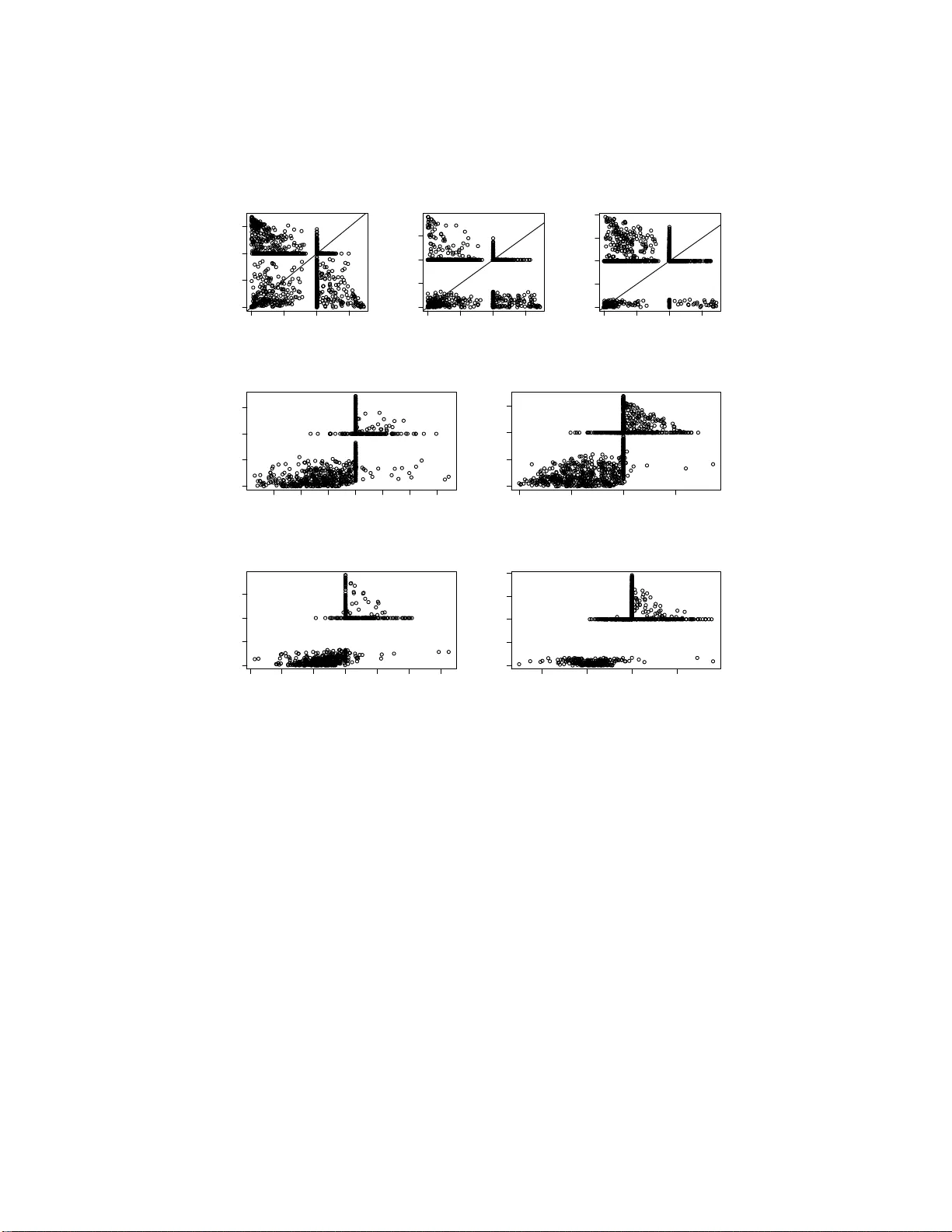
Electronic Journal of Stati stics V ol. 2 (2008) 168–212 ISSN: 1935-7524 DOI: 10.1214/ 08-EJS19 4 P en alized mo de l-based clu stering with cluster - s p e ciﬁc diagonal co v ariance matrices and group ed v ariable s Benh uai Xie and W ei P an ∗ Division of Biostatistics, Scho ol of Public He alth, Unive rsity of Minnesota e-mail: benhuaix @biostat .umn.edu ; weip@biostat .umn.edu url: www .biostat .umn.edu / ∼ weip Xiaotong She n Scho ol of Statistics, Uni versity of Minnesota e-mail: xshen@st at.umn.e du Abstract: Clustering ana lysis is one of the most widely used statistical tools in man y emerging areas suc h as microarray da ta analysis. F or microar- ray and ot her high-dimensional data, the presence of many noise v ariables may mask underlying clusteri ng structures. Hence removing noise v ariables via v ariable s election is nec essary . F or simultaneous v ariable selection and parameter estimation, existing penalized likelihoo d approac hes in model- based clustering analysis all assume a common diagonal co v ari ance matrix across clusters, whic h how ev er m a y not hold in practice. T o analyze high- dimensional data, particularly those with relativ ely lo w sample sizes, this article i ntroduces a no v el approac h that shrinks the v ariances togethe r with means, in a more general situation with cluster-sp eciﬁc (diagon al) cov ari- ance matrices. F urthermore, selection of grouped v ariables via inclusion or exclusion of a group of v ari ables altogethe r is p ermitted b y a speciﬁc form of p enalty , which facilitate s i ncorp orating s ub ject-matter knowledge, suc h as ge ne f unctions in clustering microarra y samples for di s ease subt ype disco v ery . F or implementat ion, EM algorithms are derived for parameter es- timation, in whic h t he M-steps clearly demonstrate the eﬀect s of shri nk age and thresholding. Numeri cal examples, including an application to acute leuk emia subt yp e discov ery with microarray gene expression data, are pro- vided to demonstrate the utility and ad v antage of the prop osed method. AMS 2000 sub ject classiﬁcati ons: Pr imary 62H30. Keywords and phrases: BIC, EM algorithm, H i gh-dimension but low- sample size, L 1 penalization, Micr oarr a y gene expression, Mixture model, Pe nalized likelihoo d. Receiv ed F ebruary 2008. Con ten ts 1 Int ro duction . . . . . . . . . . . . . . . . . . . . . . . . . . . . . . . . . 170 2 Metho ds . . . . . . . . . . . . . . . . . . . . . . . . . . . . . . . . . . . 172 2.1 Mixture mo del and its p enalized likelihoo d . . . . . . . . . . . . 172 ∗ Corresp onding author. 168 B. Xie et al./Penalize d mo del- b ase d clustering 169 2.2 Penalized clustering with a co mmon cov ariance matrix . . . . . . 173 2.3 Penalized clustering with unequal cov ar iance matrices . . . . . . 174 2.3.1 Regulariza tio n of v ariance pa r ameters: scheme one . . . . 174 2.3.2 Regulariza tio n of v ariance pa r ameters: scheme t w o . . . . 176 2.4 Using ada ptiv e penaliza tion to reduce bias . . . . . . . . . . . . . 177 2.5 Penalized clustering with gr oup ed v ariables . . . . . . . . . . . . 177 2.5.1 Grouping mean par ameters . . . . . . . . . . . . . . . . . 178 2.5.2 Grouping v ariance parameters . . . . . . . . . . . . . . . . 178 2.5.3 Other gro uping sc hemes . . . . . . . . . . . . . . . . . . . 179 2.6 Mo del selection . . . . . . . . . . . . . . . . . . . . . . . . . . . . 18 0 3 Sim ulations . . . . . . . . . . . . . . . . . . . . . . . . . . . . . . . . . 18 0 3.1 A common cov ar ia nce v ersus unequal cov ariances . . . . . . . . . 18 0 3.1.1 Case I . . . . . . . . . . . . . . . . . . . . . . . . . . . . . 180 3.1.2 Case I I . . . . . . . . . . . . . . . . . . . . . . . . . . . . 18 2 3.2 Grouping v ariables . . . . . . . . . . . . . . . . . . . . . . . . . . 183 4 Example . . . . . . . . . . . . . . . . . . . . . . . . . . . . . . . . . . . 183 4.1 Data . . . . . . . . . . . . . . . . . . . . . . . . . . . . . . . . . . 18 3 4.2 No gr ouping . . . . . . . . . . . . . . . . . . . . . . . . . . . . . . 184 4.2.1 Mo del-based clustering methods . . . . . . . . . . . . . . 184 4.2.2 Other clustering metho ds . . . . . . . . . . . . . . . . . . 188 4.2.3 Other compar isons . . . . . . . . . . . . . . . . . . . . . . 189 4.3 Grouping genes . . . . . . . . . . . . . . . . . . . . . . . . . . . . 19 0 5 Discussion . . . . . . . . . . . . . . . . . . . . . . . . . . . . . . . . . . 192 A Comp os ite Absolute Penalties (CAP) . . . . . . . . . . . . . . . . . . . 193 A.1 Grouping mean parameters . . . . . . . . . . . . . . . . . . . . . 193 A.2 Grouping v aria nce parameters . . . . . . . . . . . . . . . . . . . . 194 A.2.1 Scheme 1 . . . . . . . . . . . . . . . . . . . . . . . . . . . 194 A.2.2 Scheme 2 . . . . . . . . . . . . . . . . . . . . . . . . . . . 196 B Pro ofs . . . . . . . . . . . . . . . . . . . . . . . . . . . . . . . . . . . . 196 B.1 Der iv ation of Theorem 1 . . . . . . . . . . . . . . . . . . . . . . . 19 6 B.2 Der iv ation of Theorem 2 . . . . . . . . . . . . . . . . . . . . . . . 19 7 B.3 Der iv ation of ˆ σ 2 ik in section 2.3.1 . . . . . . . . . . . . . . . . . . 19 8 B.4 Der iv ation of Theorem 3 . . . . . . . . . . . . . . . . . . . . . . . 19 9 B.5 Der iv ation of ˆ σ 2 ik in section 2.3.2 . . . . . . . . . . . . . . . . . . 20 0 B.6 Der iv ation of Theorem 4 . . . . . . . . . . . . . . . . . . . . . . . 20 1 B.7 Der iv ation of Theorem 5 . . . . . . . . . . . . . . . . . . . . . . . 20 2 B.8 Cha racteriza tion of solutions to (25) . . . . . . . . . . . . . . . . 20 3 C Sim ula tion . . . . . . . . . . . . . . . . . . . . . . . . . . . . . . . . . . 203 C.1 Compar is on of the tw o regulariza tion schemes . . . . . . . . . . . 203 D Golub’s da ta . . . . . . . . . . . . . . . . . . . . . . . . . . . . . . . . 204 D.1 Compariso n of the t w o regulariz a tion schemes . . . . . . . . . . . 204 D.2 Compariso n with K im et al. (2 006)’s metho d . . . . . . . . . . . 205 Ac knowledgemen ts . . . . . . . . . . . . . . . . . . . . . . . . . . . . . . . 206 References . . . . . . . . . . . . . . . . . . . . . . . . . . . . . . . . . . . . 208 B. Xie et al./Penalize d mo del- b ase d clustering 170 1. Introduction Clustering analysis is p erhaps the most widely used analysis metho d for mi- croar ray data: it has been us ed for g ene function discovery (Eisen et a l. 1998 [ 10 ]) and cancer subtype discov ery (Golub et a l. 1999 [ 15 ]). In such an applica- tion in v olving a large num b er of g enes arrayed, it is necessary but c hallenging to c hoo se a set o f infor mative genes for clustering. If some informative ones are excluded because fewer genes are used, then it beco mes diﬃcult or imp ossible to discriminate so me phenotypes of interest such as cancer subt ypes. On the other hand, using redundant g enes introduces noise, leading to the failure to uncov er the underlying cluster ing str ucture. F or example, Alaiya et al. (20 02) [ 1 ] co n- sidered border line o v aria n tumor classiﬁcation via c lus tering protein expression proﬁles: using all 15 84 protein sp ots on a n array failed to achiev e an a ccurate classiﬁcation, while a n appropria te selection of sp ots (bas e d on discriminating betw een benign a nd malignant tumors) did giv e biologically mo re meaningful results. In spite o f its imp ortance, it is not alw ays clea r ho w to select g enes for clus- tering. In pa rticular, as demo nstrated by P an and Shen (2007) [ 39 ] and P an et al. (2006) [ 37 ], unlik e in the co nt ext of s uper vised learning, including regression, bes t subs e t selection, one of the most w ide ly used mo del selection metho ds for sup e rvised lear ning, fails for clustering and semi-supe r vised lear ning, in a ddition to its prohibitive computing cost for high-dimensional data; the reason is the existence of many corre ct models, most of which are no t of interest. In a review of the ea rlier literature o n this pr oblem, Gnana desik an et al. (199 5 ) [ 14 ] com- men ted that “ One of the thorniest a s pec ts of cluster analy sis contin ue to b e the weigh ting a nd selection of v ariables”. More recently , Raftery and Dean (2006) [ 41 ] p ointed out that “Less work has b een done on v a riable selectio n for clus- tering than for classiﬁcatio n (also called discrimina tion or sup erv ised lea rning), per haps reﬂecting the fact that the former is a harder problem. In pa rticular, v aria ble selectio n a nd dimensio n reduction in the con text o f model-ba sed clus- tering ha v e not r eceived muc h attent ion”. F o r v ariable selec tio n in mo del-based clustering, mos t of the r e cent researches fall in to tw o lines: one is Bay esian (Liu et al. 200 3 [ 30 ]; Hoﬀ 20 06 [ 18 ]; T adesse et al. 20 0 5 [ 43 ]; Kim et al. 2 006 [ 25 ]), while the other is pe na lized likelihoo d (Pan and Shen 2007 [ 39 ]; Xie et al. 2008 [ 52 ]; W ang and Zhu 2008 [ 5 0 ]). The basic statistical mo dels of these approaches are all the same: informative v ariables are a ssumed to come from a mixture of Normals, corresp onding to clusters, while noise v ar ia bles coming from a single Normal distribution; they diﬀer in how they a re implemented. In particular , the Bay esian approaches ar e more ﬂexible tha n the p enalized metho ds (because the latter a ll require a common diagonal cov ar iance ma trix, thoug h our main goal here is to relax this as sumption), but they are also computationa lly mo re demanding beca use of their use of MCMC for sto chastic sea rch; furthermore, pena lized metho ds enjoy the ﬂexibilit y of the use of p enalty functions, suc h as to accommo date gro uped para meters or v ar iables as to b e discussed later. Other recent eﬀorts include the following: Raftery and Dean (2006 ) [ 41 ] cons idered a sequential, step wise approach to v ar iable selection in model-bas e d c lus tering; B. Xie et al./Penalize d mo del- b ase d clustering 171 how ev er, as ackno wledged by the authors, “ w he n the num ber of v ar iables is v ast (e.g., in micro array data analysis when thousands of genes may be the v ariables being used), the metho d is to o slow to be pra c tical as it stands”. F riedman and Meulman (2 004) [ 11 ] dealt with a mo re general problem: selecting p ossibly diﬀerent s ubsets of v ar ia bles and their asso ciated weigh ts fo r diﬀer e n t clusters for no n-mo del-based clustering; Hoﬀ (2004) [ 17 ] po int ed out that the metho d might only “pick up the c hange in v aria nce but no t the mean”, and a dvocated the use of his mo del-based appr oach (Hoﬀ 2006 [ 18 ]). Manga sarian a nd Wild (2004) [ 3 2 ] prop osed the use of L 1 pena lt y for K-median clustering; the idea with the use of L 1 pena lt y is s imilar to our s, but we consider a more ge neral case with clus ter -sp eciﬁc v a r iance parameters. The p enalized metho ds prop osed s o far for simultaneous v aria ble selection and mo del ﬁtting in mo del-bas ed clus tering all assume a co mmon diagona l cov ariance matrix. F or high-dimensio nal data, it may be necessar y to utilize a diago nal cov ariance matrix for mo del- ba sed clustering; even for sup ervised learning, it has b een shown that using a diagonal cov ar iance ma trix in naive Bay es discriminant analysis or its v a r iants is mo r e eﬀective than that of a mor e general cov ariance matr ix (Bick el and Le v ina 2 0 04 [ 5 ]; Dudoit e t al. 200 2 [ 7 ]; Tibshirani et al. 2003 [ 47 ]). Hence w e will restrict our disc us sion to a diagonal cov ariance matrix in what follows. On the o ther hand, the c ommon (dia gonal) cov ariance matrix assumption implies that the clusters all have the same size, as in the K -means metho d (which further assumes that all the cluster s ar e sphere-shap ed with a scaled identit y matrix as the cov ariance). O f co ur se, this assumption ma y b e violated in practice. A general argument is the fo llowing: it is well known that the v aria nce of gene expression levels is in general a function of the mea n expres sion lev els, sug gesting po ssibly v arying v a riances of a gene’s expression levels across clusters with diﬀerent mean expression levels; this point is g oing to b e veriﬁed for our r e a l data example. Here we extend the metho d to allow fo r cluster-dep endent (diagonal) co v ar ia nce matrices, whic h is nontrivial and requires a suitable construction of p enalty function. In some a pplications, there is pr ior knowledge ab out grouping v ariables: some v aria bles function a s a gr o up; either all of them or none of them is informative. Y uan and Lin (2006) [ 54 ] discuss ed this is s ue in the context of p enalized r egres- sion; they demons trated convincingly the eﬃciency g ain fr om incorp or ating such prior knowledge. On the other hand, in genomic studies of clustering samples through gene expressio n proﬁles, it is kno wn that genes function in g roups as in biological pathw a ys. Hence, rather than treating genes individua lly , it seems natural to apply biolo gical knowledge o n gene functions to gr oup the g enes according ly in clustering microar ray samples, which ha s not be e n consider ed in previous applica tions of mo del-based cluster ing of expressio n proﬁles (e.g. Ghosh a nd Chinnaiyan 200 2 [ 13 ]; Li and Hong 2001 [ 27 ]; McLachlan et al. 2002 [ 33 ]; Y eung et al. 2 001 [ 5 3 ]). Note that, a few existing works clustered genes b y incorp ora ting gene function anno tations in a weak er for m that did not r equire either a ll or none of a group of genes to app e a r in a ﬁnal mo del: P an (2006b) [ 38 ] treated the genes within the same functional g roup as sharing the same prior probability o f b eing in a cluster, while genes from diﬀerent groups migh t not B. Xie et al./Penalize d mo del- b ase d clustering 172 hav e the same prior pro bability , in mo del-based clustering of genes; others to ok account of gene groups in the deﬁnition of a dista nce metric in other clustering metho ds (Huang and Pan 2006 [ 20 ]). In a dditio n, the aforementioned clustering metho ds did not allow for v ariable s election directly , while it is our ma in aim to consider v a riable selection, p os s ibly assisted with biolog ical knowledge. This is in line with the curre ntly increasing interest in incor po rating biological in- formation on gene functional groups into analy sis of detecting diﬀerential gene expression (e.g. Pan 20 06 [ 37 ]; Efron and Tibshirani 2007 [ 8 ]; Newton et al. 2007 [ 36 ]). The rest of this ar ticle is organize d as follows. Section 2 brieﬂy reviews the pena lized model- based clustering method with a common diagonal co v aria nce, follow ed b y our pr o po sed metho ds that allow for cluster-sp eciﬁc diago nal co- v aria nce ma tr ices and for g roup ed v ariables. The EM algorithms for implemen t- ing the prop osed methods are also detailed, in whic h the M-steps c haracterize the p enalize d mean a nd v a riance estimators with c lear eﬀects of shrink age and thresholding. Simulation results in section 3 and an application to real microa r - ray da ta in section 4 illustrate the utilit y of the new methods and their adv an- tages o ver other metho ds. Section 5 pr esents a summary and a shor t discussion on future work. 2. M etho ds 2.1. Mixtur e mo del and its p enalize d likeli ho o d W e hav e K -dimensiona l observ ations x j , j = 1 , . . . , n . It is a ssumed that the data have b een sta ndardized to have sample mea n 0 and sample v ar iance 1 across the n observ ations for each v ar iable. The observ ations are a ssumed to b e (marginally) iid from a mixture distribution with g compo ne nts: P g i =1 π i f i ( x j ; θ i ), where θ i is a n unknown para meter vector of the distribution for compo nen t i while π i is a prior probabilit y for comp o nent i . T o o btain the maximum penal- ized likelihoo d e s timator (MPLE), we maximize the p enalized log-likelihoo d log L P (Θ) = n X j =1 log " g X i =1 π i f i ( x j ; θ i ) # − p λ (Θ) where Θ r epresents all unk nown pa rameters and p λ (Θ) is a pe na lt y with r egular- ization par ameter λ . The speciﬁc form of p λ (Θ) dep ends on the aim of analysis . F or v a riable selection, the L 1 pena lt y is a dopted as in the Lasso (Tibshir a ni 1996 [ 46 ]). Denote b y z ij the indicator of whether x j is fro m comp onent i ; that is , z ij = 1 if x j is indeed from comp onent i , and z ij = 0 other wise. Beca use we do not obser ve which comp onent a n obser v ation comes from, z ij ’s ar e regar ded as missing da ta. If z ij ’s could b e obse rved, then the log -p enalized-likelihoo d for complete data is: log L c,P (Θ) = X i X j z ij [log π i + log f i ( x j ; θ i )] − p λ (Θ) . (1) B. Xie et al./Penalize d mo del- b ase d clustering 173 Let X = { x j : j = 1 , . . . , n } r epresent the observed data. T o max imize lo g L P , the EM algo rithm is often used (Dempster et al. 1977 [ 6 ]). The E -step o f the EM calculates Q P (Θ; Θ ( r ) ) = E Θ ( r ) (log L c,P | X ) = X i X j τ ( r ) ij [log π i + log f i ( x j ; θ i )] − p λ (Θ) , (2) while the M- step maximizes Q P to up date e stimated Θ. In the sequel, b ecause τ ij ’s a lways dep end on r , for simplicit y we may suppres s the explicit dependence from the notatio n. 2.2. Penalize d clu stering with a c omm on c ovarianc e matrix Pan and Shen (200 7) [ 39 ] speciﬁed each comp onent f i as a Nor mal distr ibution with a common dia gonal cov ariance structure V : f i ( x ; θ i ) = 1 (2 π ) K/ 2 | V | 1 / 2 exp  − 1 2 ( x − µ i ) ′ V − 1 ( x − µ i )  where V = diag ( σ 2 1 , σ 2 2 , . . . , σ 2 K ), and | V | = Q K k =1 σ 2 k . The y prop osed a p enalty function p λ (Θ) with a n L 1 norm inv olving the mean parameter s alone: p λ (Θ) = λ 1 g X i =1 K X k =1 | µ ik | , (3) where µ ik ’s are the comp onents of µ i , the mean of cluster i . Note that, because the data have b een standardized to hav e sample mean 0 and v ariance 1 for each v aria ble k , if µ 1 k = · · · = µ gk = 0, then v a riable k is no ninformative in terms of clustering a nd can b e considered as a no is e v ar iable and exc luded from the clustering analysis. The L 1 pena lt y function used in ( 3 ) can eﬀectiv ely s hr ink a small µ ik to b e exactly 0 . F or completeness and to compar e with the prop osed metho ds , w e lis t the EM upda tes to maximize the ab ov e penaliz e d likeliho o d (Pan and Shen 20 07 [ 39 ]). W e use a generic notation Θ ( r ) to r epresent the par ameter estimate at itera tion r . F o r the p oster io r probability of x j ’s coming from component i , we ha ve ˆ τ ( r ) ij = ˆ π ( r ) i f i ( x j ; ˆ θ ( r ) i ) f ( x j ; ˆ Θ ( r ) ) = ˆ π ( r ) i f i ( x j ; ˆ θ ( r ) i ) P g i =1 ˆ π ( r ) i f i ( x j ; ˆ θ ( r ) i ) , (4) for the prio r probability of an observ ation from the i th comp onent f i , ˆ π ( r +1) i = n X j =1 ˆ τ ( r ) ij /n, (5) for the v ariance for v ar iable k , ˆ σ 2 , ( r +1) k = K X k =1 n X j =1 ˆ τ ( r ) ij ( x j k − ˆ µ ( r ) ik ) 2 /n, (6) B. Xie et al./Penalize d mo del- b ase d clustering 174 and for the mea n for v ariable k in cluster i , ˆ µ ( r +1) ik = P n j =1 ˆ τ ( r ) ij x j k P n j =1 ˆ τ ( r ) ij 1 − λ 1 ˆ σ 2 , ( r ) k | P n j =1 ˆ τ ( r ) ij x j k | ! + , (7) with i = 1 , 2 , . . . , g a nd k = 1 , 2 , . . . , K . Evident ly , we hav e ˆ µ ik = 0 if λ 1 is large eno ugh. As discussed ear lier, if ˆ µ 1 k = ˆ µ 2 k = · · · = ˆ µ gk = 0 for v ariable k , v aria ble k is a noise v a riable that does not con tribute to clustering. 2.3. Penalize d clu stering with une qual c ovarianc e matric es T o allo w v arying cluster sizes , w e consider a more general mo del with cluster- depe ndent diago na l co v aria nce matrices: f i ( x ; θ i ) = 1 (2 π ) K/ 2 | V i | 1 / 2 exp  − 1 2 ( x − µ i ) ′ V − 1 i ( x − µ i )  (8) where V i = diag ( σ 2 i 1 , σ 2 i 2 , . . . , σ 2 iK ), and | V i | = Q K k =1 σ 2 ik . As dis cussed ear lier, to r ealize v a riable selection, we requir e that a noise v aria ble hav e a common mean and a commo n v ariance across clusters. Hence, the p enalty has to inv olve b oth the mean a nd v a riance parameter s. W e shall pena lize the mea n pa rameters in the sa me w ay a s b efor e , while the v ar iance parameters can b e regula rized in tw o ways: shrink σ 2 ik tow ards 1, or shrink log σ 2 ik tow ards 0. 2.3.1. R e gularization of varia nc e p ar ameters: scheme one First, we will use the followin g p enalty for b oth mean and v aria nc e parameters: p λ (Θ) = λ 1 g X i =1 K X k =1 | µ ik | + λ 2 g X i =1 K X k =1 | σ 2 ik − 1 | . (9) Again the L 1 norm is used to coer ce a small estimate of µ ik to b e exactly 0, while forcing an estimate of σ 2 ik that is close to 1 to b e exac tly 1. Therefor e, if a v a riable has common mean 0 and common v ar iance 1 across clusters, this v aria ble is eﬀectively treated as a noise v a riable; this aspect is evidenced from ( 4 ), where a noise v ar iable doe s not con tribute to the po s terior probability and th us clustering. Note that p enalty ( 9 ) diﬀers fro m the so - called double pena lization in non- parametric mixed-eﬀect models for longitudinal and other correlated data (Lin and Zhang 19 99 [ 29 ]; Gu and Ma 2005 [ 16 ]): aside fro m the ob vious diﬀerences in the choice of the L 1 -norm here versus the L 2 -norm there and in clustering here versus r egressio n ther e , they p enalized ﬁxed- and random-e ﬀect parameters , bo th mean parameters, whereas we regularize v ariance parameter s in additio n to mean pa rameters. Ma et al. (2006 ) [ 31 ] applied such a mixed-eﬀect mo del B. Xie et al./Penalize d mo del- b ase d clustering 175 to cluster genes with time course (and th us co rrelated) expression proﬁles; in addition to the aforementioned diﬀerences, a k ey diﬀerence is that their use of pena lization was for par ameter estimation, not for v a riable selectio n as aimed here. An EM a lgorithm is deriv ed as follows. The E-step giv es Q P as shown in ( 2 ). The M-s tep maximizes Q P with res p ect to the unknown para meters, resulting in the same updating fo rmulas for τ ij and π i as given in ( 4 ) and ( 5 ). In Appendix B , we derive the following theorem: Theorem 1. The suﬃcient and ne c essary c onditio ns for ˆ µ ik to b e a (glob al) maximizer of Q P ar e P n j =1 τ ij x j k P n j =1 τ ij = λ 1 σ 2 ik P n j =1 τ ij + | ˆ µ ik | ! sign ( ˆ µ ik ) , if and only if ˆ µ ik 6 = 0 (10) and       n X j =1 τ ij x j k       /σ 2 ik ≤ λ 1 , if and only if ˆ µ ik = 0 , (11) r esu lting in a slightly change d formula for t he me an p ar ameters ˆ µ ( r +1) ik = P n j =1 ˆ τ ( r ) ij x j k P n j =1 ˆ τ ( r ) ij 1 − λ 1 ˆ σ 2 , ( r ) ik | P n j =1 ˆ τ ( r ) ij x j k | ! + . (12) F or the v ariance pa rameters, some alg ebra yields the following theorem: Theorem 2. The ne c essary c onditions for ˆ σ 2 ik to b e a lo c al maximizer of Q P ar e n X j =1 τ ij  − 1 2 ˆ σ 2 ik + ( x j k − ˆ µ ik ) 2 2 ˆ σ 4 ik  = λ 2 sign ( ˆ σ 2 ik − 1) , if ˆ σ 2 ik 6 = 1 (13) and       n X j =1 τ ij  − 1 2 + ( x j k − ˆ µ ik ) 2 2        ≤ λ 2 , if ˆ σ 2 ik = 1 . (14) Although a suﬃcient condition for ˆ σ 2 ik = 1 can be derived as a sp ecial cas e of Theo r em 5 , we do not have an y suﬃcien t condition for ˆ σ 2 ik 6 = 1. Hence, w e do no t ha v e a simple form ula to up date ˆ σ 2 ik . Belo w we c haracterize the solution ˆ σ 2 ik , suggesting a computational a lgorithm as well as illustrating the eﬀects o f shrink a ge. Let a ik = λ 2 sign( ˆ σ 2 ik − 1), b i = P n j =1 τ ij / 2, and c ik = P n j =1 τ ij ( x j k − ˆ µ ik ) 2 / 2, then ( 13 ) reduces to a ik σ 4 ik + b i σ 2 ik − c ik = 0, while ( 14 ) b ecomes | b i − c ik | ≤ λ 2 . Note that ˜ σ 2 ik = c ik /b i is the usual ML E when λ 2 = 0. It is easy to verify that if ˜ σ 2 ik = 1, then ˆ σ 2 ik = 1. Below we consider cases with λ 2 > 0 and ˜ σ 2 ik 6 = 1. It is shown in App endix B that B. Xie et al./Penalize d mo del- b ase d clustering 176 1. if | b i − c ik | > λ 2 , ˆ σ 2 ik = ˜ σ 2 ik 1 2 + r 1 4 + sign ( c ik − b i ) λ 2 c ik b 2 i (15) is the unique maximizer of Q P and is b etw een 1 and ˜ σ 2 ik ; 2. if | b i − c ik | ≤ λ 2 , (a) if ˜ σ 2 ik > 1, then ˆ σ 2 ik = 1 is the unique maximizer; (b) if ˜ σ 2 ik < 1, i) if b i − c ik < λ 2 , then ˆ σ 2 ik = 1 is a local maximizer; there may exist another loca l maximizer betw een ˜ σ 2 ik and 1 ; b e t w een the t wo, the one maximizing Q P is chosen; ii) if b i − c ik = λ 2 , then either ˆ σ 2 ik = c ik /λ 2 ∈ ( ˜ σ 2 ik , 1) (if ˜ σ 2 ik < 1 / 2 ) or ˆ σ 2 ik = 1 (if ˜ σ 2 ik ≥ 1 / 2 ) is the unique maximizer . Naturally the ab ov e for m ulas sugg est an updating algorithm for σ 2 ik . Clearly , ˆ σ 2 ik has b een shrunk tow ards 1, and can b e exactly 1 if, for ex ample, λ 2 is suﬃciently large. 2.3.2. R e gularization of varia nc e p ar ameters: scheme two The following penalty is adopted for both mea n and v ariance parameters: p λ (Θ) = λ 1 g X i =1 K X k =1 | µ ik | + λ 2 g X i =1 K X k =1 | log σ 2 ik | . (16) Note that the only diﬀerence betw een ( 9 ) and ( 16 ) is the penalty of the v a riance parameters , where | σ 2 ik − 1 | is r e placed by | log σ 2 ik | , which is used to shr ink log σ 2 ik to 0 (i.e. σ 2 ik to 1) if log σ 2 ik is close to 0. Ther efore, v aria ble selection can be realized as b efore. An EM algorithm for the v ar iance para meters is derived as follows. Theorem 3. The suﬃcient and ne c essary c onditions for ˆ σ 2 ik to b e a lo c al max- imizer of Q P ar e n X j =1 τ ij  − 1 2 ˆ σ 2 ik + ( x j k − ˆ µ ik ) 2 2 ˆ σ 4 ik  = λ 2 sign (log ˆ σ 2 ik ) ˆ σ 2 ik , if ˆ σ 2 ik 6 = 1 (17) and       n X j =1 τ ij  − 1 2 + ( x j k − ˆ µ ik ) 2 2        ≤ λ 2 , if ˆ σ 2 ik = 1 . (18) If we denote b i = P n j =1 τ ij / 2 and c ik = P n j =1 τ ij ( x j k − ˆ µ ik ) 2 / 2, then ( 17 ) reduces to ˜ σ 2 ik = ˆ σ 2 ik (1 + λ 2 sign(log ˆ σ 2 ik ) /b i ), while ( 18 ) b ecomes | b i − c ik | ≤ λ 2 , where ˜ σ 2 ik = c ik /b i is the usual MLE for λ 2 = 0. Deriv ations in App endix B B. Xie et al./Penalize d mo del- b ase d clustering 177 imply that sign(log ˆ σ 2 ik ) = sign(log ˜ σ 2 ik ) = sign( c ik − b i ). Combining the t wo cases, we obtain ˆ σ 2 ik =  ˜ σ 2 ik 1 + λ 2 sign( c ik − b i ) /b i − 1  sign( | b i − c ik | − λ 2 ) + + 1 (19) The above formula sug gests an updating algor ithm for σ 2 ik . When λ 2 is small, sign( | b i − c ik | − λ 2 ) + = 1 , ˆ σ 2 ik has b een shrunk from ˜ σ 2 ik tow ards 1; when λ 2 is suﬃciently la rge, sign( | b i − c ik | − λ 2 ) + = 0, then ˆ σ 2 ik is exa c tly 1. 2.4. Using adaptive p enalization to r e duc e bi as W e can adopt the idea of a daptive penaliza tio n, as propo sed by Zou (2006) [ 57 ] for regress io n, in the present context. F ollowing Pan et al. (2006 ) [ 40 ], w e use a weigh ted L 1 pena lt y function p λ (Θ) = λ 1 g X i =1 K X k =1 w ik | µ ik | + λ 2 g X i =1 K X k =1 v ik | σ 2 ik − 1 | , (20) where w ik = 1 / | ˆ µ ik | w and v ik = 1 / | ˆ σ 2 ik − 1 | w with w ≥ 0, and ˆ µ ik and ˆ σ 2 ik are the MPLE obta ine d in section 2.3.1 ; w e also tried the usual MLE in w ik and v ik , but it did not work well in simulations, hence we s kip its dis cussion; w e only consider w = 1. The EM up dates are slightly mo diﬁed for the purpo se: w e only need to replace λ 1 and λ 2 by λ 1 w ik and λ 2 v ik resp ectively , while k eeping other upda tes unchanged. The main idea of adaptive p enalizatio n is to reduce the bias o f the MPLE asso ciated with the standard L 1 pena lt y: as can be seen clearly , if an initia l estimate | ˆ µ ik | is larger , then the res ulting estimate is shrunk less tow ards 0; similarly for the v ariance para meter. 2.5. Penalize d clu stering with gr oup e d variables Now we consider a situation where candidate v ariables can be gro uped bas e d on the pr ior b elief that either all the v ar iables in the same group or none of them are informative to clustering. F ollowing the same idea o f the g r oup ed Lasso of Y uan a nd Lin (200 6) [ 54 ], we construct a p enalty for this purp os e here. Suppo se that the v aria bles ar e par titioned into M gro ups with the c o r- resp onding mean parameters µ i = ( µ i 1 , µ i 2 , . . . , µ iK ) ′ = ( µ 1 i ′ , µ 2 i ′ , . . . , µ M i ′ ) ′ , dim( µ m i ) = k m , and P M m =1 k m = K . Accordingly , w e de c ompo se x j = ( x 1 j ′ , x 2 j ′ , . . . , x M j ′ ) ′ and V i = diag ( σ 2 i 1 , σ 2 i 2 , . . . , σ 2 iK ) = diag ( V i 1 , V i 2 , . . . , V iM ) with V im as a k m × k m diagonal ma trix, and σ 2 i,m is the column vector containing the diagonal elements of matrix V im . F or g rouping mean par ameters, we w ill use a pe nalty p λ (Θ) containing λ 1 g X i =1 M X m =1 p k m k µ m i k B. Xie et al./Penalize d mo del- b ase d clustering 178 for the mean para meters, where k v k is the L 2 norm of vector v . Accordingly , we use λ 2 g X i =1 M X m =1 p k m k σ 2 i,m − 1 k as a p enalty for group ed v aria nce parameter s. Note that we do not have to group both means a nd v ariances at the same time. F or instance, we ma y group only means but not v a riances: w e will th us use the second term in ( 9 ) as the pena lt y for v ariance parameters while reta ining the ab ove penalty for g roup ed mean parameter s. The E-step of the EM yields Q P with the same for m a s ( 2 ). Next we derive the up dating for mulas for the mean and v a riance parameters in the M-step. 2.5.1. Gr ouping me an p ar ameters If the p enalty for group ed means is used, we ha v e the following result. Theorem 4 . The suﬃcient and ne c essary c ondi tions fo r µ = ( µ m i ) , i = 1 , 2 , . . . , g and m = 1 , 2 , . . . , M t o b e a unique maximizer of Q P ar e V − 1 im   n X j =1 τ ij x m j − n X j =1 τ ij ! µ m i   = λ 1 p k m µ m i k µ m i k , if and only if µ m i 6 = 0 , (21) and       n X j =1 τ ij x m j ′ V − 1 im       ≤ λ 1 p k m , if and only if µ m i = 0 , (22) yielding ˆ µ m i = sign 1 − λ 1 √ k m k P n j =1 τ ij x m j ′ V − 1 im k !! + ν m i ˜ µ m i (23) wher e ν m i =  I + λ 1 √ k m P n j =1 τ ij k ˆ µ m i k V im  − 1 , and ˜ µ m i = P n j =1 τ ij x m j / P n j =1 τ ij is the usual MLE. It is clear that, due to thresholding, ˆ µ m i = 0 when, for example, λ 1 is suﬃ- ciently la rge. Noting that ν m i depe nds on ˆ µ m i , we use ( 23 ) iteratively to update ˆ µ m i . 2.5.2. Gr ouping varianc e p ar ameters If the p enalty for group ed v ariances is used, we hav e the follo wing theorem: B. Xie et al./Penalize d mo del- b ase d clustering 179 Theorem 5 . The suﬃcient and ne c essary c ondi tions fo r σ 2 i,m = 1 , i = 1 , 2 , . . . , g and m = 1 , 2 , . . . , M , to b e a lo c al maximizer of Q P ar e                   n X j =1 τ ij  1 2 1 − 1 2 ( x m j − µ m i ) 2       ≤ λ 2 p k m if n X j =1 τ ij  1 2 1 − ( x m j − µ m i ) 2  ≤ 0 ;      n X j =1 τ ij  1 2 1 − 1 2 ( x m j − µ m i ) 2       < λ 2 p k m otherwise. (24) The n e c essary c ondition for σ 2 i,m 6 = 1 to b e a lo c al maximizer of Q P is n X j =1 τ ij " − 1 2 σ 2 i,m + 1 2( σ 2 i,m ) 2 ( x m j − µ m i ) 2 # = λ 2 √ k m ( σ 2 i,m − 1 ) k σ 2 i,m − 1 k . (25) It is clea r that σ 2 i,m = 1 when, for exa mple, λ 2 is lar ge enough. It is also easy to verify that ( 24 ) a nd ( 25 ) r educe to the same ones for non-gro uped v aria bles w he n k m = 1. T o solve ( 24 ) and ( 25 ), we develop the fo llowing algorithm. Let a im = λ 2 √ k m / k σ 2 i,m − 1 k , b i = ( P n j =1 τ ij / 2) 1 and c im = P n j =1 τ ij ( x m j − µ m i ) 2 / 2. Consider an y k ′ th comp onent σ 2 ik ′ of σ 2 i,m ; cor r esp ond- ingly , b ik ′ and c imk ′ are the k ′ th comp onents o f b i and c im , resp ectively . In Appendix B , treating a im as a constant (i.e. b y plug ging-in a curre nt estimate of σ 2 i,m ), we s how the following cases. i) If ˜ σ 2 ik ′ = 1, then ˆ σ 2 ik ′ = 1 is a maximizer of Q P as other σ 2 ik ’s for ∀ k 6 = k ′ are ﬁxed. ii) If ˜ σ 2 ik ′ = c imk ′ /b ik ′ > 1, ther e exists only one r eal ro ot satisfying ˆ σ 2 ik ′ ∈ (1 , ˜ σ 2 ik ′ ); a bis e ction sea rch ca n be used to ﬁnd the ro o t. iii) If ˜ σ 2 ik ′ = c imk ′ /b ik ′ < 1, the real ro ots m ust b e inside ( ˜ σ 2 ik ′ , 1), hence a bisection sear ch can b e used to ﬁnd a ro ot; once a r o ot is obtained, the other t w o real ro o ts, if exist, can be obtained through a closed-for m expression; we c ho ose the real ro ot that maximizes Q P (while other σ 2 ik for k 6 = k ′ are ﬁxed at their current estimates) as the new estimate of σ 2 ik ′ . After cy c ling through all k ′ , we update a im with the new estimate. Then the ab ove pro cess is iterated. 2.5.3. Other gr ouping schemes T o sav e space, we brieﬂy discuss grouping v ariables under a common diag o nal cov a riance matrix, fo r which only mean pa rameters need to b e regularized. The EM up dating formula for the mean par ameters remains the same as in ( 23 ) except that the cluster- spe c iﬁc cov a riance V im there is replaced by a common V m ; upda ting formulas for the other para meters remain unc hanged. Sim ulation results (see Xie et al. (2008) [ 52 ]) demonstra ted its improv ed p erfor mance ov er its c o unt erpart without grouping . In addition, we can also group the mean parameters for the same v aria ble (or gene) across clusters (W ang and Zhu 2008 [ 50 ]), and combine it with g rouping v ar iables (Xie et al. 2 008 [ 52 ]). The gr ouping scheme discussed so fa r follows the group ed La sso of Y ua n and Lin (2006 ) [ 54 ], which is a sp ecia l case of the Comp o site Absolute Penalties (CAP) of Zhao et al. (2 006) [ 56 ]. In Appe ndix A , w e derive the results with the CAP , including using both sc hemes on regular izing the v ar iance parameters. B. Xie et al./Penalize d mo del- b ase d clustering 180 2.6. Mo del sele ction T o introduce pena lization, following Pan and Shen (2007) [ 39 ] and Pan e t a l. (2006) [ 40 ], we prop ose a mo diﬁed BIC as the mo del sele c tion criterion: B I C = − 2 log L ( ˆ Θ) + log( n ) d e where d e = g + K + g K − 1 − q is the eﬀective num ber of parameters with q = # { ( i , k ) : µ ik = 0 , σ 2 ik = 1 } . The deﬁnition of d e follows fr om that in L 1 - pena lized regression (Efro n e t al. 2004 [ 9 ]; Zou et al. 2004 [ 59 ]). This modiﬁed BIC is used to select the num ber of clusters g and the penaliza tio n parameters ( λ 1 , λ 2 ) jointly . W e prop ose using a gr id sear ch to es timate the optimal ( g , ˆ λ 1 , ˆ λ 2 ) as the o ne w ith the minim um BIC. F or any given ( g , λ 1 , λ 2 ), b ecause of p ossibly many lo cal maxima for the mixture mo del, we run a n EM algorithm m ultiple times with random sta rts. F or our n umerical examples, we randomly started the K -means and used the K-means’ results as an initializa tion for the EM. F rom the multiple runs, we selected the o ne g iving the maximal pena lized log-likelihoo d a s the ﬁnal result for the given ( g , λ 1 , λ 2 ). 3. Si m ulations 3.1. A c ommon c ovarianc e versus une qual c ovarianc es 3.1.1. Case I W e ﬁr st considered fo ur simple set-ups: the ﬁrs t was a null case with g = 1; for the other three, g = 2 , corres p o nding to only mea n, only v a r iance, and bo th mean and v ariance diﬀerences b etw een the tw o cluster s. Sp e ciﬁcally , we generated 100 sim ulated datasets for each set-up. In each da taset, there w ere n = 100 obser v ations , each of whic h co n tained K = 300 v a riables. Set-up 1 ) is a null case: all the v ariables had a sta nda rd normal distribution N (0 , 1), thus there w as only a sing le c luster. F or each o f the other three set-ups, there w ere t wo clusters. One clus ter cont ained 8 0 o bs erv a tio ns while the other contained 20; while 2 79 v aria bles were noises distr ibuted as N (0 , 1), the other 21 v a riables were informa tiv e: each of the 21 v ariables were distributed as 2) N (0 , 1 ) in cluster 1 versus N (1 . 5 , 1) in cluster 2; 3) N (0 , 1) versus N (0 , 2); 4) N (0 , 1) versus N (1 . 5 , 2) for the thr e e set-ups resp ectively . F or ea ch simulated dataset, we ﬁtted a series of mo dels with the three num- ber s o f components g = 1, 2, 3 and v a rious v alues of p enaliza tion par ameter(s). F or compariso n, we considere d bo th the e qual cov ar iance and unequal cov ar i- ance mixture mo dels ( 8 ); for the former, w e considered the unpenalized method ( λ 1 = 0) co rresp onding to no v ariable selection and p enaliz e d metho d using BIC to select λ ; similarly , for the la tter w e considered ﬁv e cases corresp onding to ﬁx- ing or selecting one or tw o of ( λ 1 , λ 2 ): no v ariable selection with ( λ 1 , λ 2 ) = (0 , 0 ), B. Xie et al./Penalize d mo del- b ase d clustering 181 T a ble 1 Simulation c ase I: fr e quencie s of the sele cte d numb ers ( g ) of clusters, and me an numb ers of pr e dicte d noise variables among the true informative ( z 1 ) and noise variables ( z 2 ). Her e N 1 and N 2 wer e the fr equencies of sele cting Une qualCo v( ˆ λ 1 , ˆ λ 2 ) (with varianc e r e g ularization scheme one) and EqualCov( ˆ λ 1 ) by BIC, r esp ectively. Une qualCov( ˆ λ 1 , ˆ λ 2 ) (lo gvar) use d varianc e r e gularization scheme two. F or set-up 1, the truth was g = 1 , z 1 = 21 and z 2 = 279 ; for others, g = 2 , z 1 = 0 and z 2 = 279 UnequalCo v( λ 1 , λ 2 ) EqualCo v( λ 1 ) BIC (0 , 0) ( ˆ λ 1 , 0) (0 , ˆ λ 2 ) ( ˆ λ 1 , ˆ λ 2 ) ( ˆ λ 1 , ˆ λ 2 )(logv ar) (0) ( ˆ λ 1 ) Set-up g N N N N z 1 z 2 N z 1 z 2 N N z 1 z 2 N 1 N 2 1 99 83 99 100 21.0 279 .0 100 21.0 279.0 100 100 21.0 279.0 0 100 1 2 0 3 0 0 - - 0 - - 0 0 - - 0 0 3 1 14 1 0 - - 0 - - 0 0 - - 0 0 1 99 89 99 - - - - - - 100 0 - - 0 0 2 2 0 1 0 100 0.03 276.0 100 0.03 276.0 0 87 0.03 275.1 0 87 3 1 10 1 - - - - - - 0 13 9.8 0.0 0 13 1 97 74 97 52 21.0 279.0 43 21.0 279.0 100 100 21.0 279.0 48 4 3 2 0 3 0 42 5.4 276.8 48 3.4 275.1 0 0 - - 42 0 3 3 23 3 6 6.8 277.8 9 3.6 276.3 0 0 - - 6 0 1 97 74 97 0 - - 0 - - 100 4 21.0 279.0 0 0 4 2 0 3 0 98 0.2 275.9 97 0.1 275.2 0 88 2.9 276.2 90 2 3 3 23 3 2 0.5 276.5 3 0.3 274.0 0 8 6.0 276.8 8 0 1 100 100 10 0 52 21.0 279.0 51 21.0 279.0 100 100 21.0 279.0 0 63 3 2 0 0 0 38 2.5 277.4 40 2.1 275.0 0 0 - - 34 0 (adapt) 3 0 0 0 10 3.5 277.6 9 3.4 275.4 0 0 - - 3 0 pena lizing only mea n parameter s with ( λ 1 , λ 2 ) = ( ˆ λ 1 , 0), p enalizing only v ar i- ance parameters with ( λ 1 , λ 2 ) = (0 , ˆ λ 2 ), and our pr o p o sed t w o metho ds of p e - nalizing b oth mean a nd v ar iance parameters with ( λ 1 , λ 2 ) = ( ˆ λ 1 , ˆ λ 2 ). W e also compared the num b ers of predic ted no ise v ariables among the true 2 1 infor ma - tive ( z 1 ) and 279 noise v aria bles ( z 2 ). The frequencies of s electing g = 1 to 3 based on 100 simulated datasets are shown in T able 1 . Fir st, our prop osed methods p erfor med b est, in general, in terms of selecting b oth the correc t num ber of clus ters and relev an t v ariables. F or example, it selected fewest noise v ariables and most informative v a riables. Second, no v ariable selection (i.e. no p enaliz a tion) led to inc o rrectly selecting g = 1 for the three non-null set-ups. Third, penalizing only the mean para meter s could not distinguish the tw o clusters diﬀer ing o nly in v a riance as in set-up 3. F ourth, b etw een the tw o reg ularization s chemes for the v ariance parameter s, based on b oth cluster detection and sample assignment (T able 2 ), the tw o gav e comparable r esults, though scheme t w o with log- v ariance pe r formed slig ht ly better . The results for a daptive penalty for set-up 3 are detailed in row 3(adapt) of T a ble 1 , whic h a re similar to that of using the L 1 -norm penalty in terms of bo th v ariable and cluster n um ber se le c tion. Since the perfor mance of a daptive pena lt y might heavily dep end on the choice of weights (or initial estimates), w e exp ect improved p erformance if better w eigh ts c a n be used. B. Xie et al./Penalize d mo del- b ase d clustering 182 T a ble 2 Sample assignments for ˆ g = 2 and (adjuste d) R and index (RI/aRI) values for t he two r egul arization schemes for the varianc e p ar ameters for simulation set-ups 2-4. # Corr r epr esents the ave r age numb er of the samples fr om a true c luster c orr e ctly assigne d to an estimate d cluster Sample assignmen ts, Rand Index ˆ g = 2 Cluster 1 Cluster 2 ( n = 80) ( n = 20) ˆ g = 1 ˆ g = 2 ˆ g = 3 Ov erall Set-up Methods #Corr # Corr RI aRI RI aRI RI aRI RI aRI L 1 (v ar-1) 78.8 19.0 - - 1.00 0.99 - - 1.00 0.99 2 L 1 (logv ar) 78.8 19.0 - - 1.00 0.99 - - 1.00 0.99 L 1 (v ar-1) 74.6 15.1 0.68 0.0 0.89 0.75 0.87 0.70 0.78 0.36 3 L 1 (logv ar) 76.9 16.6 0.68 0.0 0.94 0.85 0.95 0.88 0.83 0.49 L 1 (v ar-1) 78.4 19.0 - - 0.99 0.98 0.97 0.93 0. 99 0.98 4 L 1 (logv ar) 78.8 19.0 - - 1.00 0.99 0.99 0.98 1.00 0.99 T a ble 3 Simulation c ase II. The me an numb ers of the pr edicte d noise variables as in e ach of the ﬁrst thr ee gr oups of true inf ormative and the other gr oup of noise variables wer e given by z 1 - z 4 ; the trut h was that g = 2 , z 1 = z 2 = z 3 = 0 and z 4 = 300 − 3 K 1 UnequalCo v( λ 1 , λ 2 ) EqualCo v( λ 1 ) (0 , 0) ( ˆ λ 1 , 0) (0 , ˆ λ 2 ) ( ˆ λ 1 , ˆ λ 2 ) (0) ( ˆ λ 1 ) K 1 g N N N N z 1 z 2 z 3 z 4 N N z 1 z 2 z 3 z 4 1 96 76 96 48 5.0 5.0 5.0 285.0 100 74 5.0 5.0 5.0 285 5 2 0 1 0 42 2.0 1.8 1.5 283.5 0 15 0.0 4.5 0.5 279.7 3 4 23 4 10 0.2 0.4 0.0 283.9 0 11 0.0 4.2 0.3 279.5 1 96 81 96 11 7.0 7.0 7.0 279.0 100 26 7.0 7.0 7.0 279 7 2 2 4 2 81 0.8 1.0 0.5 276.5 0 54 0.0 6.3 0.7 274.7 3 2 15 2 8 0.0 0.6 0.0 277.0 0 20 0.0 6.6 0.6 275.3 1 99 86 99 0 - - - - 100 1 10.0 10.0 10.0 270.0 10 2 0 2 0 94 0.2 0.9 0.1 266.3 0 81 0.01 9.0 0.8 266.6 3 1 12 1 6 0.0 0.3 0.0 266.8 0 18 0.0 9.1 0.7 267.6 3.1.2. Case II W e conside r ed a mo re practical scenario that combined clus ter s’ diﬀerences in means or v aria nc e s o r b oth for informative v ar iables. As before, for each dataset, n = 100 observ ations w ere divided in to t wo clusters with 80 a nd 20 observ ations resp ectively; among the K = 300 v ariables, only 3 K 1 were informative while the remaining K − 3 K 1 were noises; The ﬁr st, second and third K 1 informative v aria bles w ere distributed as i) N (0 , 1) for cluster 1 v ersus N (1 . 5 , 1) for cluster 2, ii) N (0 , 1) versus N (0 , 2), iii) N (0 , 1) versus N (1 . 5 , 2), resp ectively; an y noise v aria ble w as distributed N (0 , 1 ). W e co ns idered K 1 = 5 , 7, and 10 . The r e s ults are s hown in T able 3 . Again it is clear tha t our propo sed metho d work ed best: it most frequently selected the corr ect num ber of clusters ( g = 2), and used most informa tiv e v ariables while being able to weed out most noise v ariables. As exp ected, using noise v ariables, as in non-p enalized methods without v ar iable selection, tended to mask out the existence of the t w o clusters. B. Xie et al./Penalize d mo del- b ase d clustering 183 T a ble 4 Simulation c ase II for gr ou p e d variables Grouping means only Means and v ariances K 1 g N z 1 z 2 z 3 z 4 N z 1 z 2 z 3 z 4 1 21 5.0 5.0 5.0 285.0 14 5. 0 5.0 5.0 285.0 5 2 62 0.2 0.5 0.2 283.4 71 0. 0 0.0 0.0 284.6 3 17 0.0 0.7 0.0 283.2 15 0. 0 0.0 0.0 284.7 1 2 7.0 7.0 7.0 279.0 1 7.0 7.0 7.0 279.0 7 2 90 0.0 0.6 0.0 277.4 92 0. 0 0.0 0.0 278.9 3 8 0.0 0.8 0.0 277.4 7 0.0 0.0 0.0 279.0 1 0 - - - - 0 - - - - 10 2 96 0.0 0.7 0.0 268.3 98 0. 0 0.0 0.0 269.8 3 4 0.0 0.8 0.0 266.8 2 0.0 0.0 0.0 270.0 3.2. Gr ouping var iables W e gro upe d v ar iables fo r ea ch simulated data under ca s e I I. W e used c orrect groupings: the informative v aria bles w ere gro upe d together, and so were the noise v ar iables; the gro up sizes were 5, 7 and 5 for K 1 = 5, 7 and 10 r esp ectively . T able 4 displays the results for group ed v ariables . Compa r ed to T able 1 , it is clear that gro uping v a riables improv ed the perfo rmance ov er no n- group ed one in terms of more frequently selecting the corre c t num ber g = 2 of the clus ters as w ell as better selecting relev an t v ariables. F ur thermore, grouping both mea ns and v ar iances per formed b etter than grouping means alone. 4. E xample 4.1. Data A leukemia gene expression dataset (Golub et al. 1999 [ 15 ]) was used to demon- strate the utilit y of our prop osed method a nd to co mpare with other meth- o ds. The (training) data co n tained 38 patients, among which 11 w ere AML (acute my eloid leukemia) while the r e maining were ALL (acute lymphoblas- tic leukemia) samples ; ALL samples co ns isted of tw o subtypes: 8 T-cell and 19 B-cell samples. F o r each sa mple, the express io n levels of 7129 genes were measured by an Aﬀymetrix microarray . F ollowing Dudoit et al. (2002) [ 7 ], we pre-pro cess ed the data in the follo wing steps: 1) truncation: any expressio n lev el x j k was truncated b elow at 1 if x j k < 1, and above at 16,000 if x j k > 16 , 000; 2) ﬁltering: an y gene w as excluded if its max/min ≤ 5 a nd ma x − min ≤ 5 00, where max and min were the maximum and minimum express io n lev els of the gene across all the samples. Finally , as a preliminary gene screening, w e selected the top 200 0 genes with the largest sample v aria nces acro s s the 38 samples. B. Xie et al./Penalize d mo del- b ase d clustering 184 T a ble 5 Clustering r esults for Golub’s data wit h t he numb er of c omp onents ( g ) sele cted by BIC UnequalCo v( λ 1 , λ 2 ) EqualCo v( λ 1 ) Methods (0 , 0) ( ˆ λ 1 , ˆ λ 2 ) (0) ( ˆ λ 1 ) RI/aRI 0 . 73 / 0 . 46 0 . 85 / 0 . 65 0 . 70 / 0 . 37 0 . 70 / 0 . 25 BIC 71225 52198 75411 6 3756 Clusters 1 2 1 2 3 4 1 2 3 1 2 3 4 5 6 7 8 9 10 11 Samples(#) ALL-T(8) 8 0 0 0 8 0 8 0 0 7 0 0 0 0 0 1 0 0 0 0 ALL-B(19) 17 2 11 1 0 7 0 8 11 0 4 5 2 4 0 0 1 1 1 1 AML(11) 0 11 0 11 0 0 0 0 11 0 0 0 0 7 4 0 0 0 0 0 4.2. No gr ou ping 4.2.1. Mo del-b ase d clustering metho ds T able 5 displays the clustering r esults: the tw o p enalized metho ds selected 4 and 11 clusters, resp ectively , while the tw o standa rd methods chose 2 and 3 clusters, res pectively . F or the new pena liz e d metho d, we show the results for scheme one of regularizing the v ariance parameter s ; the other scheme and the adaptive p enaliza tio n both gave s imilar results, and hence are skipp e d. In terms of discriminating be t w een the luekemia subt ypes, o b viously the new pena lized metho d p erfor med best: only one ALL B-ce ll sa mple was mixed into the AML group, while others formed homogeneo us groups. In contrast, with a large nu m- ber o f clusters, the L 1 metho d with an equal co v ariance still misclassiﬁed 4 ALL B-cell samples as AML. The tw o standard metho ds p erhaps under-s e lected the nu m ber of clusters, re s ulting in 11 a nd 10 mis-classiﬁed samples, res pectively . Unsurprisingly , based on the Rand index (Rand 1971 [ 42 ]) (or a djusted Rand index (Hubert a nd Arabie 1 985 [ 22 ])), the new method was a winner with the largest v alue at 0 . 8 5 (0.65), compa red to 0 . 73 (0.46), 0 . 70 (0.3 7) and 0 . 7 0 (0.25) of the o ther three metho ds. In addition, judged by BIC, the new p enalized metho d also outp erfor med the other metho ds with the smalle s t BIC v alue of 52198 . Fina lly , the new penalized method used o nly 17 28 genes, while p e nalizing only means with a co mmon cov ariance matrix used 1821 genes; the other tw o standard metho ds used all 2000 genes. Figure 1 displays the es timated means and v a riances o f the genes in diﬀerent clusters. Panels a)-c) clea rly sho w that the genes ma y ha ve diﬀeren t v aria nce estimates across the clusters , though many of them w ere shrunk to b e exactly to be one, as exp ected. Note that, due to the standa r dization of the data yielding an overall sample v a riance one for each gene, w e do not obser ve a ny gene with the v ariance estimates more than o ne in tw o or mor e cluster s . Panels d)-f ) conﬁrmed that there appea rs a monotonic rela tionship betw een the mean and v aria nce, as w ell-kno wn in the microarr ay litera ture (e.g. Huang and Pan 2 002 [ 19 ]); the Pearson co rrelation coeﬃcients w ere estimated to be 0 . 6 4, 0 . 69, 0 . 65 and 0 . 63 for the four clusters resp ectively . Hence, it lends an indirect supp or t for the use of cluster-sp eciﬁc co v ariance matrices: if it is accepted that the genes B. Xie et al./Penalize d mo del- b ase d clustering 185 0.0 0.5 1.0 1.5 0.0 0.5 1.0 1.5 σ ^ 1 2 σ ^ 2 2 a) 0.0 0.5 1.0 1.5 0.0 0.5 1.0 1.5 σ ^ 1 2 σ ^ 3 2 b) 0.0 0.5 1.0 1.5 0.0 0.5 1.0 1.5 2.0 σ ^ 1 2 σ ^ 4 2 c) −0.6 −0.4 −0.2 0.0 0.2 0.4 0.6 0.0 0.5 1.0 1.5 µ ^ 1 σ ^ 1 2 d) −1.0 −0.5 0.0 0.5 0.0 0.5 1.0 1.5 µ ^ 2 σ ^ 2 2 e) −1.5 −1.0 −0.5 0.0 0.5 1.0 1.5 0.0 0.5 1.0 1.5 µ ^ 3 σ ^ 3 2 f) −1.0 −0.5 0.0 0.5 0.0 0.5 1.0 1.5 2.0 µ ^ 4 σ ^ 4 2 g) Fig 1 . Sca tter plots of the estimate d me ans and varianc es b y t he new p e nalize d metho d. Panels a)–c) ar e sca tter plots of the estimate d varianc es in cluster 1 versus those in cluster 2, 3 and 4, resp ectively; p anels d)–g) ar e the sc atter plots of the estimate d me ans ve rsus est imate d varianc es for the four clusters r esp e ctively. hav e v arying mean para meters across cluster s, then their v ariance parameters are exp ected to c hange too. Next w e examine a few genes in more details. CST3 (cystatin c, M23197) and ZYX (zyxin, X95735) were in the top 50 genes ranked b y Golub et al. (19 99) [ 15 ], and t w o of the 17 genes selected by Antono v et al. (2004 ) [ 2 ] to discriminate betw een the AML/ALL subt yp e s. In addition, the tw o genes, together with MAL (X76223), were a ls o identiﬁed among the top 20 genes used in the class iﬁer by Liao et al. (2 007) [ 28 ] to predict leukemia s ubt ypes . Ba rdi et al. (200 4) [ 4 ] used CST3 to assess glomerular function a mong children with leukemia and solid tumors and found that CST3 was a suitable marker. Ko o et al. (200 6) [ 26 ] reviewed the liter ature s howing the relev ance of MAL to T- c ell ALL and concluded that it might pla y an imp o rtant role in T-cell a ctiv ations. Baker et B. Xie et al./Penalize d mo del- b ase d clustering 186 −1 0 1 2 3 −1 0 1 2 3 Unequal covariances a) All samples CST3 MAL ALL − T ALL − B AML Cluster 1 Cluster 2 Cluster 3 Cluster 4 −1 0 1 2 3 −1 0 1 2 3 Equal covariance b) All samples CST3 MAL Cluster 1 Cluster 2 Cluster 3 Cluster 4 Cluster 5 Cluster 6 Cluster 7−11 −0.65 −0.60 −0.55 −0.50 −0.45 −0.55 −0.45 −0.35 Unequal covariances c) Zoom−in of a) CST3 MAL −0.60 −0.55 −0.50 −0.45 −0.40 −0.35 −0.30 −0.50 −0.46 −0.42 −0.38 Equal covariance d) Zoom−in of b) CST3 MAL −1 0 1 2 3 −1 0 1 2 3 4 Unequal covariances e) All samples ZYX LCK −1 0 1 2 3 −1 0 1 2 3 4 Equal covariance f) All samples ZYX LCK Fig 2 . Observe d expr ession lev els of two p airs of genes and t he c orr esp onding clusters f ound by the two p enalize d metho ds. al. (2 006) [ 3 ] a nd W a ng et al. (2005) [ 49 ] ident iﬁed ZYX as the most signiﬁcant gene for classifying AML/ALL subtypes. Tyc k o et al. (19 91) [ 48 ] found that LCK (M26692) was related to a c tiv ated T cells and th us it might co n tribute to the for mation of human cancer . W r ight et al. (1 994) [ 51 ] studied the mutation of LCK and concluded that it proba bly pla yed a ro le in some human T-cell leukemia. In Figure 2 , panels c )– d ) a r e the zo om-in versions of the left b ottom of a )– b ), the plots of g e ne pa ir CST3 and MAL for a ll samples for the tw o pena lized B. Xie et al./Penalize d mo del- b ase d clustering 187 −0.5 0.0 0.5 1.0 −0.6 −0.2 0.2 0.6 Sample mean µ ^ 1 a) 0.0 1.0 2.0 3.0 0.0 0.5 1.0 1.5 Sample variance σ ^ 1 2 b) Fig 3 . Penalize d me an and varianc e estimates f or cluster one co ntaining the 11 ALL B-c el l samples by the new p enalize d metho d. metho ds resp ectively , w hile e )– f ) a re for gene pair LCK and Z YX with a ll samples. Given t w o genes, their observed expression levels, a long with the 9 5 % conﬁdence reg ion of the center for each cluster , were plotted. T he p enalized metho d with an equal cov a riance found 11 cluster s, among which 5 clus ter s had only o ne sample, and the remaining 6 clusters ha d more than 2 samples; for clarity , w e only plotted the conﬁdence r e gions of the c e nters of the six large s t clusters. Panels a) and e) clear ly sho w evidence of v ary ing v aria nces, and thus cluster-sp eciﬁc cov aria nce matr ices: for example, MAL was hig hly expres sed with a larg e disp ers ion for ALL-T samples, so w as CST3 fo r AML samples, in con trast to the low expressio n o f b oth genes for ALL-B sa mples , s ug gesting v ary ing cluster sizes. It also clearly illustrates wh y there were so many clus ters if an equa l cov aria nc e mo del was used: the large num ber of the equally - sized clusters were used to approximate the three o r four siz e-v ar ying true cluster s. Panel c) also sugg ests an ex pla nation to the use of tw o clusters fo r ALL-B samples b y the new p enalized metho d: the expr ession lev els of MAL and CST3 were p os itively correla ted, giving a cluster not parallel with either co ordinate; on the other hand, use of a diago nal cov a riance matrix in the penalized metho d implied a cluster parallel to one of the t w o co o rdinates. Hence, t wo co or dinate- parallel cluster s were needed to a ppr oximate the non-co or dinate-para lle l true cluster; a no n-diagona l cov ar iance matrix might give a more pa rsimonious mo del (i.e. with fewer clusters). Finally , w e show the eﬀects o f shrink age and thresholding for the par ameter estimates b y the new p enalized metho d. Figure 3 depicts the penalized mean estimates (panel a) and v a riance estimates (panel b) v ersus the sample means B. Xie et al./Penalize d mo del- b ase d clustering 188 T a ble 6 Clustering r esults for Golu b’s data b y P AM and K -me ans metho ds. The numb er of clusters sele c te d by t he si lhouette width ar e maske d by * Methods P A M K-means RI/aRI 0 . 46 / 0 0 . 65 / 0 . 24 0 . 64 / 0 . 22 0 . 67 / 0 . 27 0 . 80 / 0 . 53 0 . 75 / 0 . 42 Clusters 1 2* 1 2 3 1 2 3 4 1 2 3 1 2 3 4 1 2 3 4 5 6* Samples (#) ALL-T (8) 7 1 1 7 0 1 7 0 0 5 3 0 0 0 8 0 0 0 0 0 8 0 ALL-B (19) 11 8 8 3 8 8 3 7 1 10 7 2 10 2 0 7 1 9 0 8 0 1 AML (11) 11 0 11 0 0 11 0 9 0 0 1 10 0 10 0 1 0 4 7 0 0 0 and v a riances resp ectively for cluster one. It is co nﬁrmed that the p enalized mean es timates were shrunk to w ards 0, s ome of whic h were exactly 0, while the pena lized v ar iance estimates were shrunk tow ards 1, and can b e ex a ctly 1. 4.2.2. Other clustering metho ds Previous studies (e.g. Thalam uth u et a l. 2006 [ 44 ]) hav e established model-based clustering as one of the bes t p erformer s for gene expr ession data . Although it is not our main g o al her e, a s a comparison in passing, we show the r esults o f other three widely used metho ds as applied to the s ame da ta with the top 200 0 genes: hiera rchical c lustering, par titioning a r ound medoids (P AM) and K-means clustering. It is c hallenging to determine the num ber of clusters for P AM and K -means. Here we co nsider tw o pro p o s als. First, w e used the silhouette width (Ka ufman and Rousseeuw 1990 [ 24 ]) to select the num ber of clusters. Two and six clusters were c hosen for P AM and K-means resp ectively; neither gav e a go o d sepa r ation among the three le ukemia subtypes (T able 6 ). Second, to sidestep the is s ue, w e applied the tw o metho ds with three and four clusters b ecause thos e n um ber s seemed to work b est for mo del-based cluster ing. Nevertheless, P AM worked po o rly , w hile K- means with 4 cluster s gave a reasona ble result, a lbe it not as go o d as that of the new pena lized mo del-bas ed clustering, a s judged b y an eye-ball ex a mination or the (adjusted) Rand index. Figure 4 gives the r esults of hiera rchical clustering with all three wa ys of deﬁning a cluster-to-cluster dis tance: av e r age link age, sing le link age and co m- plete link a g e. The average link age clustering g av e the b e st separation among the three leukemia subtypes : all 8 T-cell samples , except sa mple 7, were g roup ed together; there w ere 10 B-cell samples in a group; all other ALL samples seemed to a ppea r in the AML gro up. On the other hand, the av erage link ag e cluster ing ident iﬁed ab out s ix outlying samples, whic h w ere samples 7, 18, 19, 21, 22 and 27 resp ectively; this ﬁnding was consistent with that of the p enalized mo del- based clustering with an equal cov a riance matrix, whic h detected the same ﬁv e outliers except sa mple 19. B. Xie et al./Penalize d mo del- b ase d clustering 189 1 2 3 8 5 4 6 9 10 12 11 16 24 15 17 20 26 14 25 28 31 34 35 32 13 23 7 19 27 29 37 38 33 30 36 18 21 22 50 70 90 110 Average linkage clustering Sample Height 1 2 3 8 5 10 12 4 6 17 20 26 14 25 31 34 35 9 11 16 24 15 28 32 23 29 13 7 30 36 27 37 19 38 33 21 18 22 50 70 90 Single linkage clustering Sample Height 1 14 25 28 31 32 30 36 29 37 38 33 2 3 8 5 4 6 7 11 16 24 15 17 20 26 19 9 10 12 13 23 34 35 27 18 21 22 40 60 80 120 Complete linkage clustering Sample Height Fig 4 . A gglomer ative hier ar chic al cluste ri ng r esults for the 38 leukemia samples: the ﬁrst 8 samples wer e T-c el l ALL ; samples 9-27 wer e B-c el l AL L; the r e maining ones wer e AML . 4.2.3. Other c omp ariso ns Although mainly studied in the co nt ext of sup ervised lear ning, with several existing studies, Golub’s da ta ma y serve as a test bed to c o mpare v ar io us clus- tering metho ds. Golub et al. (1999) [ 15 ] applied self-orga niz ing maps (SOM): ﬁrst, with tw o c lusters, SOM mis-classiﬁed one AML and 3 ALL samples; sec- ond, with four clusters , similar to the result of o ur new penalized metho d, AML and ALL-T each formed a clus ter while ALL-B for med tw o clusters, in which one ALL-B and one AML s amples w ere mis-classiﬁed. They did not discuss why or ho w g = 2 or g = 4 clusters were c hosen. In Bay esian mo del-based clustering by Liu et al. (2003) [ 30 ], t wo clus ters were chosen with one AML a nd one ALL mis-assigne d; they did not discuss classiﬁcatio n with ALL subtypes. In a very rece n t s tudy by Kim et al. (2006) [ 25 ], with t wo clustering alg o- rithms a nd tw o c hoices of a prior para meter, they present ed four sets of clus- tering results. In general, ALL sa mples formed o ne cluster while AML samples formed 5 to 6 clusters , giving 0-3 mis-assigned ALL sa mples; although not dis- cuss explicitly , b ecause either all or almos t a ll the ALL samples fell in to one cluster, their method obviously could not dis tinguish the t w o s ubt ypes of ALL. F urthermor e, their result o n the m ultiple clusters of AML was in contrast to B. Xie et al./Penalize d mo del- b ase d clustering 190 ours and Golub’s on the homogeneity o f AML samples. Becaus e K im et al. used diﬀerent data pre-pro cessing with 3 571 genes as input to their metho d, for a fair compariso n, we applied the same dataset to our new penalized metho d, yielding ﬁve clusters: only one ALL-B was mis- assigned to a cluster con taining 10 AML samples, one clus ter w as co ns isted o f o ne ALL- B and AML samples, while the other three c lusters contained 8 ALL-T, 10 ALL- B and 7 ALL- B resp ectively . F or this dataset, our metho d se e med to work better. It w as somewha t sur prising that there were ab out 1800 g enes rema ining for the pena lized metho ds, though previous studies showed that there were a lar g e nu m ber of the ge ne s diﬀerentially express ed between ALL and AML; in par - ticular, Golub et a l. (1999) [ 15 ] stated that “ r oughly 1100 genes were mor e highly co rrelated with the AML-ALL class distinction than would be exp ected by chance”; see also Pan and Shen (2 0 07) [ 39 ] and r eferences therein. F or a simple ev a luation, we applied the elas tic net (Zou and Hastie 20 05 [ 58 ]) to the same data with top 2000 genes; the elastic net is a state-of-the-ar t supervis ed learning metho d sp eciﬁcally designed for v ariable selection for high-dimensiona l data a nd is implemented in R pack age elasti cnet . Fiv e-fold cr oss-v alidation was used for tuning parameter selection. As us ual, w e decompos ed the three- class pro ble m in to tw o binary classiﬁers, ALL-T v s AML, and ALL-B vs ALL, resp ectively . The t wo cla ssiﬁers eliminated 395 and 870 noise genes, resp ectively , with a c ommon set of 227 genes. Hence the elastic net used 1773 g enes, a num ber comparable to those s e lected by the pena lized clustering methods. 4.3. Gr ouping genes The 2000 g enes were group ed accor ding to the Kyoto Encyclop edia of Genes and Genomes (KEGG) Pathw a y database (Kanehisa and Goto 2000 [ 23 ]). Ab out 43 per cent of the 2000 genes b elonged to at least one of 126 K EGG path wa ys. If a gene w as in more than one path w ay , it w as randomly assigned to o ne of the pathw ays to which it belong ed. Ea ch g enes un-annotated in any pathw a y w as treated as an individual gro up with size 1. Among the 126 KEGG pathw a ys, the larges t pa th wa y size w as 44, the smallest one was 1 and the median size was 4; ab out three quarters of the pathw ays had size s less than 8. The clustering results with the gr oup e d mean and v a riance pena lization were exactly the same as that of UnequalCov and kept 179 5 genes. Among the 205 ident iﬁed no ise g e nes, 23 genes were fro m 17 KEGG path wa ys: all contained only one ge ne s exce pt only three pathw ays, each con taining 2, 3 a nd 4 genes resp ectively . T o further ev aluate the above gene selection results, we sear ched a Leukemia Gene Databa se containing ab out 70 genes that w ere previo usly identiﬁed in the literature as leukemia-related ( www.bi oinfo rmatics.org/legend/leuk_db.htm ). Among these informative genes, 58 were related to 21 leuk emia subtypes, among which only 47 and 3 6 genes appea r ed in the whole Golub’s data and the 333 7 genes after prepr o cessing res pectively . Among the top 2000 genes b eing used for clustering, there w ere only 30 genes in the Leukemia Gene Databa se, most B. Xie et al./Penalize d mo del- b ase d clustering 191 T a ble 7 The genes in the L eukemia Gene Datab ase that wer e r etaine d in or r emove d fr om the ﬁnal mo del for the gr oup e d metho d. The six genes in italic font wer e annotate d in KEGG p athways Leuk emia Subt ype Gene Name Acute Lymphoblastic Leuk emia MYC , ZNFN1A1 Acute Myeloge nous Leuke mia IRF1, GMPS Acute Myeloid Leukemia CBFB, NUP214, HOXA9, FUS, RUNX1 Acute Promy elocytic Leuk emia PML Acute Undiﬀerent iated Leuk emia SET B-cell Chronic Lymphocytic Leuk emi a BCL3, BTG1 Mye loid Leuk emia CLC Retained pre B-cell Leuk emia PBX1, PBX3 T-cell Leuk emia TCL6 T-cell Acute Lymphoblastic Leuk emia NOTCH3 , L YL1, LMO2, T AL2 Cutaneous T-cell Leuk emia NFKB2 Human Monocytic Leuk emi a ETS1 Mast cell Leuk emia KIT Mixed Link age Le uk emia MLL3 Acute Myeloid Leukemia LCP1 Acute Myeloge nous Leuke mia RGS2 Remo v ed Murine Myeloid Leuk emi a EVI2B pre B-cell Leuk emia PBX2 T-cell Leuk emia TRA@ of which w ere not in any KEGG pathw a ys; o nly 7 g enes app eared in KEGG pathw ays: GMPS, E TS1, NOTCH3, MLL3, MYC, NFKB2 and K IT . T able 7 lists the g enes that were selected in and de le ted from the ﬁnal model. Among the 2 05 noise genes s elected b y our g roup p enalized metho d, ﬁve of them w ere annotated in the Leukemia Gene Database, among whic h o ne was rela ted to AML. Because most of the kno wn leukemia genes w ere no t in an y K E GG path w ays, reﬂecting p erha ps the curren t lack of pr ior knowledge, the group ed metho d co uld not b e established as a clea r winner ov er the none-gr oup ed method in terms of leukemia gene sele ction in the a bove example. T o co nﬁrm the potential gain with a better use of prio r knowledge, w e did t w o a dditional exp eriments. Fir st, in ad- dition to the KEGG path w ays, we group ed a ll the 1 9 leukemia genes not in any KEGG path w ays into a separa te group: the samples were clustered as b efore; among the 200 genes removed from the ﬁnal mo del, there were only t wo leukemia gene, ETS1, which w as related to h uman mono cytic leukemia, neither AML nor ALL, and NOTCH3, related to T-ce ll ALL. Second, in addition to the KEGG pathw ays, w e g roup ed the AML (“acute m y eloid leuk emia” in T able 7 ) or ALL (“acute lymphoblastic leukemia” a nd “ T-cell acute lymphoblas tic leukemia”) genes in to tw o co r resp onding gr oups while trea ting the other leukemia g enes individually: aga in the samples were clustered as befor e; among the 216 genes remov ed from the ﬁnal mo del, ETS1, RGS2, E VI2B, PBX2, TRA@ were the four leuk emia genes and there w as no single gene related to AML or ALL. These t wo ex per iment s demonstrated the eﬀectiv eness of g rouping genes based on bi- B. Xie et al./Penalize d mo del- b ase d clustering 192 ologica l knowledge, and that, as exp ected, the quality of the prio r knowledge would inﬂuence p erformanc e . Nevertheless, our work her e is just a ﬁrst step, and mor e r esearch is necessa ry to establish the practical use of grouping g enes for microa rray data. 5. Di scussion W e ha v e prop osed a new pe nalized likelihoo d method for v a riable sele c tio n in mo del-based clustering, p ermitting cluster- de p endent diago na l cov ariance ma- trices. A ma jor nov elt y is the developmen t of a new L 1 pena lt y inv olving b oth mean and v ariance par ameters. The p enalized mixture mo del can b e ﬁtted easily using an EM alg orithm. Our numerical studies demonstrate the utilit y of the prop osed method and its sup e rior p erformance ov er o ther methods. In particular, it is conﬁrmed tha t for high-dimensio nal data such as ar ising from microarr ay exp eriments, v ariable selection is necessary: without v ariable selec- tion, the presence of a large num ber of noise v a r iables c a n mask the clustering structure under lying the da ta. F ur thermore, w e hav e also studied penalties for group ed v ar iables to inco rp orate prior k nowledge into clustering a nalysis, which, as ex p ected, improv es per formance if the pr ior k nowledge being used is indeed informative. The present approach inv o lves only diagonal cov ar ia nce matrices. It is ar gued that for “ high dimension but small sample size” settings as ar ising in g enomic studies, the w orking indep endence as s umption is eﬀective, as sugg e sted by F ra- ley and Raftery (2 006) [ 12 ], as well as demonstrated by the po pular use of a diagonal cov ar iance matrix in the naiv e Bayes a nd o ther discr imina n t a nalyses due to its go o d p erfor ma nce (Bick el and Levina 20 0 4 [ 5 ]; Dudoit et al. 2 002 [ 7 ]; Tibshir ani et al. 2 003 [ 47 ]). Nev ertheless, it is worthwhile to g e neralize the prop osed a pproach to other non-diagonal cov aria nce matrices, possibly built on the no v el idea of shrinking v ar iance components as prop osed here. Howev er, this task is muc h mor e c hallenging; a main diﬃculty is ho w to guarantee a s hrunk cov a riance matr ix to be po sitive deﬁnite, as evidenced b y the c hallenge in a sim- pler context of pena lized estimation of a single co v aria nce matrix (Huang et al. 2006 [ 21 ]; Y uan and Lin 2007 [ 55 ]). An alternative approach is to hav e a mo del int ermediate betw een the indep endent and unrestricted mo dels. F or example, in a mixture o f factor analyzers (McLa chlan et al. 2 003 [ 35 ]), local dimension reduction within each component is realized throug h so me latent factors, which are also used to explain the correlations among the v a riables. Nevertheless, b e- cause the laten t factors are assumed to be shared by all the v ariables while in fact they may only be related to a small subset o f informative v ar iables, v ar i- able selection may still be necessary; how ev er, how to do so is an open ques tion. Finally , although our propo sed p enalty for gr oup ed v ar iables provides a gene r al framework to co nsider a g r oup of genes, e.g. in a relev a nt biological pathw ay or functional gr oup, for their either “all in” or “a ll out” prop erty in clustering, there remain some pr actical questio ns, such as how to cho ose pathw ays and how to handle genes in m ultiple pathw ays. Thes e interesting topics remain to be studied. B. Xie et al./Penalize d mo del- b ase d clustering 193 App endix A: Comp osite Absolute P enalties (CAP) W e generalize our proposed group penalization, including the tw o r egulariza tion schemes on v a riance parameters, to the Compo site Absolute P enalties (CAP) of Zhao et al. (2006 ) [ 56 ], which covers the gr oup penalty of Y uan and Lin (20 06) [ 54 ] as a special ca s e. F or grouping mean para meters, the following penalty function is used for the mean parameter s: λ 1 g X i =1 M X m =1 k γ 0 /γ ′ m m k µ m i k γ 0 γ m ! 1 /γ 0 (26) where 1 / γ m + 1 /γ ′ m = 1, γ m > 1 and k v k γ m is the L γ m norm of vector v . Accordingly , w e adopt λ 2 g X i =1 M X m =1 k γ 0 /γ ′ m m k σ 2 i,m − 1 k γ 0 γ m ! 1 /γ 0 (27) or λ 2 g X i =1 M X m =1 k γ 0 /γ ′ m m k log σ 2 i,m k γ 0 γ m ! 1 /γ 0 (28) as a penalty for group ed v ar iance parameters. T o achiev e sparcit y , as usual, w e use γ 0 = 1. The E-step of the EM yields Q P with the same for m a s ( 2 ). Next we derive the up dating for mulas for the mean and v a riance parameters in the M-step. A.1. Gr oupi ng me an p ar ameters If the CAP p enalty function ( 26 ) for group e d means is used, we can der ive the following Theo rem: Theorem 6 . The suﬃcient and ne c essary c ondi tions fo r µ = ( µ m i ) , i = 1 , 2 , . . . , g and m = 1 , 2 , . . . , M , to b e a unique maximizer of Q P ar e V − 1 im   n X j =1 τ ij x m j −   n X j =1 τ ij   µ m i   = λ 1 k 1 /γ ′ m m sign ( µ m i ) | µ m i | γ m − 1 k µ m i k γ m − 1 γ m , if and only if µ m i 6 = 0 , (29) and       n X j =1 τ ij x m j ′ V − 1 im       γ ′ m ≤ λ 1 k 1 /γ ′ m m , if and only if µ m i = 0 , (30) yielding ˆ µ m i = sign 1 − λ 1 k 1 /γ ′ m m k P n j =1 τ ij x m j ′ V − 1 im k γ ′ m !! + ν m i ˜ µ m i (31) B. Xie et al./Penalize d mo del- b ase d clustering 194 wher e ν m i =  I + λ 1 k 1 /γ ′ m m k ˆ µ m i k γ m − 2 P n j =1 τ ij k ˆ µ m i k γ m V im  − 1 , and ˜ µ m i = P n j =1 τ ij x m j / P n j =1 τ ij is the usual MLE. Pr o of. Co nsider t wo ca ses: i) µ m i 6 = 0 . Firs t, by deﬁnition and using the H¨ older’s inequality , w e can prov e that the L γ m norm is conv ex, th us the p enalty function for gr o uped means is conv ex in µ m i . Seco nd, treating Q P as the Lagrange multiplier for a constrained optimization problem w ith the p enalty as the inequality co nstraint, and con- sidering that b oth min us the o b jectiv e function and the penalty function are conv ex, b y the K arush-Kuhn- T uck er (KKT ) condition, we have the following suﬃcient and necessary condition ∂ Q P /∂ µ m i = 0 ⇐ ⇒ X j τ ij V − 1 im ( x m j − µ m i ) − λ 1 k 1 /γ ′ m m sign( µ m i ) | µ m i | γ m − 1 k µ m i k γ m − 1 γ m = 0 , from which w e can easily ge t ( 29 ). ii) µ m i = 0 . By deﬁnition, we hav e Q P ( 0 , . ) ≥ Q P (∆ µ m i , . ) for any ∆ µ m i close to 0 ⇐ ⇒ − X j τ ij 1 2 ( x m j ) ′ V − 1 im x m j + C 1 ≥ − X j τ ij 1 2 ( x m j − ∆ µ m i ) ′ V − 1 im ( x m j − ∆ µ m i ) − λ 1 k 1 /γ ′ m m || ∆ µ m i || γ m + C 1 ⇐ ⇒ X j τ ij x m j ′ V − 1 im ∆ µ m i / || ∆ µ m i || γ m − X j τ ij (∆ µ m i ) ′ V − 1 im ∆ µ m i / (2 || ∆ µ m i || γ m ) ≤ λ 1 k 1 /γ ′ m m . Notice P j τ ij (∆ µ m i ) ′ V − 1 im ∆ µ m i / (2 || ∆ µ m i || γ m ) → 0 + as ∆ µ m i → 0 . By the H¨ o lde r ’s inequality , we hav e    P j τ ij x m j ′ V − 1 im ∆ µ m i / || ∆ µ m i || γ m    ≤ || P j τ ij x m j ′ V − 1 im || γ ′ m , and the ” = ” can b e attained. Th us the ab ov e ineq uality is equiv alent to ( 30 ). It is clear that, if λ 1 is large enough, ˆ µ m i will b e exactly 0 due to thresholding . Since ν m i depe nds on ˆ µ m i , we use ( 31 ) iter atively to update ˆ µ m i . A.2. Gr oupi ng varianc e p ar ameters A.2.1. Scheme 1 If the p enalty function ( 27 ) for group ed v ariance s is used, we ha ve the following theorem: B. Xie et al./Penalize d mo del- b ase d clustering 195 Theorem 7 . The suﬃcient and ne c essary c ondi tions fo r σ 2 i,m = 1 , i = 1 , 2 , . . . , g and m = 1 , 2 , . . . , M , to b e a lo c al maximizer of Q P ar e                   n X j =1 τ ij  1 2 1 − 1 2 ( x m j − µ m i ) 2      γ ′ m ≤ λ 2 k 1 /γ ′ m m if n X j =1 τ ij  1 2 1 − ( x m j − µ m i ) 2  ≤ 0 ;      n X j =1 τ ij  1 2 1 − 1 2 ( x m j − µ m i ) 2       γ ′ m < λ 2 k 1 /γ ′ m m otherwise. (32) The n e c essary c ondition for σ 2 i,m 6 = 1 to b e a lo c al maximizer of Q P is n X j =1 τ ij " − 1 2 σ 2 i,m + 1 2( σ 2 i,m ) 2 ( x m j − µ m i ) 2 # = λ 2 k 1 /γ ′ m m sign ( σ 2 i,m − 1 ) | σ 2 i,m − 1 | γ m − 1 k σ 2 i,m − 1 k γ m − 1 γ m . (33) Pr o of. If σ 2 i,m = 1 is a lo ca l maxim um, by deﬁnition, we hav e the following suﬃcient and necessary condition Q P ( 1 , . ) ≥ Q P ( 1 + ∆ σ 2 i,m , . ) for any ∆ σ 2 i,m near 0 ⇐ ⇒ X j τ ij  − 1 2 ( x m j − µ m i ) ′ ( x m j − µ m i )  + C 1 ≥ X j τ ij  − 1 2 log | diag( 1 + ∆ σ 2 i,m ) | − 1 2 ( x m j − µ m i ) ′ diag( 1 + ∆ σ 2 i,m ) − 1 ( x m j − µ m i )  − λ 2 k 1 /γ ′ m m || ∆ σ 2 i,m || γ m + C 1 . Thu s, X j τ ij  − 1 2 log | diag( 1 + ∆ σ 2 i,m ) | + 1 2 ( x m j − µ m i ) ′ diag(∆ σ 2 i,m / ( 1 + ∆ σ 2 i,m ))( x m j − µ m i )  ≤ λ 2 k 1 /γ ′ m m || ∆ σ 2 i,m || γ m . Using T aylor’s expansion, we hav e n X j =1 τ ij − 1 2 1 + ( x m j − µ m i ) 2 2 ! ′ ∆ σ 2 i,m + 1 2 n X j =1 τ ij  1 2 1 − ( x m j − µ m i ) 2  ′ (∆ σ 2 i,m ) 2 + O  c ′ (∆ σ 2 i,m ) 3  ≤ λ 2 k 1 /γ ′ m m || ∆ σ 2 i,m || γ m for so me consta nt vector c . After dividing b oth sides by || ∆ σ 2 i,m || γ m and using the same ar gument as b efore, we obtain ( 32 ) as the suﬃcient and necessar y condition for σ 2 i,m = 1 to b e a local ma ximizer of Q P . B. Xie et al./Penalize d mo del- b ase d clustering 196 Setting the ﬁrst-order der iv ative of Q P equal to 0, we hav e ( 33 ), the necessary condition for σ 2 i,m 6 = 1 to b e a local ma ximizer of Q P . It is clear that we have σ 2 i,m = 1 when, for example, λ 2 is large enough. It is also easy to v erify that the abov e co nditio ns reduce to the same o nes for σ 2 ik = 1 for non-gro uped v ar iables when k m = 1 and reduce to ( 24 ) and ( 25 ) for group ed v aria bles when γ m = γ ′ m = 2. A.2.2. Scheme 2 If we use the CAP p enalty function ( 28 ) for g r oup ed v a riances, then the following theorem can b e o btained by a similar ar g ument as b efore: Theorem 8 . The suﬃcient and ne c essary c ondi tions fo r σ 2 i,m = 1 , i = 1 , 2 , . . . , g and m = 1 , 2 , . . . , M , to b e a lo c al maximizer of Q P ar e                 n X j =1 τ ij  1 2 1 − 1 2 ( x m j − µ m i ) 2       γ ′ m ≤ λ 2 k 1 /γ ′ m m if n X j =1 τ ij  1 2 1 − ( x m j − µ m i ) 2  ≤ 0 ;      n X j =1 τ ij  1 2 1 − 1 2 ( x m j − µ m i ) 2       γ ′ m < λ 2 k 1 /γ ′ m m otherwise. (34) The n e c essary c ondition for σ 2 i,m 6 = 1 to b e a lo c al maximizer of Q P is n X j =1 τ ij " − 1 2 σ 2 i,m + 1 2( σ 2 i,m ) 2 ( x m j − µ m i ) 2 # = λ 2 k 1 /γ ′ m m sign (log σ 2 i,m ) | log σ 2 i,m | γ m − 1 k log σ 2 i,m k γ m − 1 γ m . (35) App endix B: Pro ofs B.1. Derivation of The or em 1 Since Q P is diﬀerentiable with respect to µ ik when µ ik 6 = 0, while non-diﬀeren- tiable at µ ik = 0, we c onsider the fo llowing t wo ca ses: i) If µ ik 6 = 0 is a maxim um, given that Q P is co ncav e and diﬀeren tiable, then the suﬃcient and necess a ry condition for µ ik to b e the global maximum of Q P is ∂ Q P /∂ µ ik = 0 ⇐ ⇒ n X j =1 τ ij ( x j k − µ ik ) /σ 2 ik − λ 1 sign( µ ik ) = 0 , from which w e hav e ( 10 ). ii) If µ ik = 0 is a ma x im um, we c ompare Q P (0 , . ) with Q P (∆ µ ik , . ), the v a lues of Q P at µ ik = 0 a nd µ ik = ∆ µ ik resp ectively (while o ther co mp onents of µ i B. Xie et al./Penalize d mo del- b ase d clustering 197 are ﬁxed at its maxim um). By deﬁnition, we hav e Q P (0 , . ) ≥ Q P (∆ µ ik , . ) for any ∆ µ ik near 0 ⇐ ⇒ − X j τ ij 1 2 x 2 j k /σ 2 ik + C 1 ≥ − X j τ ij 1 2 ( x j k − ∆ µ ik ) 2 /σ 2 ik − λ 1 | ∆ µ ik | + C 1 ⇐ ⇒ X j τ ij 1 2 (2 x j k sign(∆ µ ik ) − | ∆ µ ik | ) /σ 2 ik ≤ λ 1 ⇐ ⇒    X j τ ij x j k    /σ 2 ik ≤ λ 1 as ∆ µ ik → 0 . It is o bvious that from ( 10 ) w e have sign( µ ik ) = sign( P n j =1 τ ij x j k / P n j =1 τ ij ), th us µ ik = P n j =1 τ ij x j k P n j =1 τ ij 1 − λ 1 σ 2 ik sign( µ ik ) P n j =1 τ ij x j k ! = P n j =1 τ ij x j k P n j =1 τ ij 1 − λ 1 σ 2 ik | P n j =1 τ ij x j k | ! , which, in com bination with ( 11 ), yields ( 12 ). B.2. Derivation of The or em 2 Since Q P is diﬀeren tiable with resp e ct to σ 2 ik when σ 2 ik 6 = 1 , w e know a loca l maximum ˆ σ 2 ik m ust satisfy the follo wing conditions      ∂ ∂ σ 2 ik Q P (Θ; Θ ( r ) ) | σ 2 ik = ˆ σ 2 ik = 0 if ˆ σ 2 ik 6 = 1; Q P (1 , . ) ≥ Q P (1 + ∆ σ 2 ik , . ) if ˆ σ 2 ik = 1and for any ∆ σ 2 ik near 0 . (36) where . in Q P (1 , . ) repr esents all parameters in Q P except σ 2 ik . Notice tha t Q P = C 1 + P j τ ij  − 1 2 log σ 2 ik + C 2 − 1 2 ( x j k − µ ik ) 2 /σ 2 ik  − λ 2 | σ 2 ik − 1 | + C 3 , whe r e C 1 , C 2 and C 3 are constan ts with respect to σ 2 ik . The r efore the ﬁrst equation of ( 36 ) b ecomes n X j =1 τ ij  − 1 2 ˆ σ 2 ik + ( x j k − µ ik ) 2 2 ˆ σ 4 ik  − λ 2 sign( ˆ σ 2 ik − 1) = 0 , if ˆ σ 2 ik 6 = 1 from which w e can easily ge t ( 13 ). Starting from the second equation of ( 36 ), we hav e LHS = C 1 + X j τ ij  − 1 2 log(1) + C 2 − 1 2 ( x j k − µ ik ) 2 / 1  − λ 2 | 1 − 1 | + C 3 , RHS = C 1 + X j τ ij  − 1 2 log(1 + ∆ σ 2 ik ) + C 2 − 1 2 ( x j k − µ ik ) 2 / (1 + ∆ σ 2 ik )  − λ 2 | ∆ σ 2 ik | + C 3 , B. Xie et al./Penalize d mo del- b ase d clustering 198 and thus 1 2 X j τ ij  − log(1 + ∆ σ 2 ik ) − ( x j k − µ ik ) 2 (1 / (1 + ∆ σ 2 ik ) − 1 )  ≤ λ 2 | ∆ σ 2 ik | . Using T aylor’s expansion, we hav e n X j =1 τ ij  − 1 2 + ( x j k − µ ik ) 2 2  ∆ σ 2 ik + O ((∆ σ 2 ik ) 2 ) ≤ λ 2 | ∆ σ 2 ik | , leading to n X j =1 τ ij  − 1 2 + ( x j k − µ ik ) 2 2  sign(∆ σ 2 ik ) + O ( | ∆ σ 2 ik | ) ≤ λ 2 . letting ∆ σ 2 ik → 0, we obta in (14). B.3. Derivation of ˆ σ 2 ik in se ction 2.3.1 Note that from ( 13 ) we hav e ( − ∂ Q P /∂ σ 2 ik ) σ 4 ik = a ik σ 4 ik + b i σ 2 ik − c ik = 0. Deﬁne f ( x ) = a ik x 2 + b i x − c ik = 0. First, we consider the ca se with | b i − c ik | ≤ λ 2 . i ) When ˜ σ 2 ik > 1, f ( ˜ σ 2 ik ) = a ik ˜ σ 4 ik + 0 = λ 2 ˜ σ 4 ik > 0, and f ( x ) = λ 2 sign( x − 1) x 2 + b i x − c ik = λ 2 x 2 + b i x − c ik > b i x − c ik ≥ b i ˜ σ 2 ik − c ik = 0 if x > ˜ σ 2 ik > 1. On the other hand, lim x → 1 + f ( x ) = λ 2 + b i − c ik ≥ 0, since | b i − c ik | ≤ λ 2 ; and f ( x ) = − λ 2 x 2 + b i x − c ik < − λ 2 x 2 + b i − c ik < 0 if x < 1 . Thus, based on the signs of f ( x ), Q P has a unique local max im um at ˆ σ 2 ik = 1. ii ) When ˜ σ 2 ik < 1, w e ha v e f ( ˜ σ 2 ik ) = − λ 2 ˜ σ 4 ik < 0, and f ( x ) = − λ 2 x 2 + b i x − c ik < b i x − c ik < b i ˜ σ 2 ik − c ik = 0 if x < ˜ σ 2 ik ; lim x → 1 − f ( x ) = − λ 2 + b i − c ik ≤ 0; and f ( x ) = λ 2 x 2 + b i x − c i > λ 2 + b i − c i > 0 if x > 1. How ev er, fo r ˜ σ 2 ik < x < 1 , f ( x ) = − λ 2 x 2 + b i x − c ik is a contin uous a nd quadr a tic function, which may hav e tw o ro ots x 1 , 2 = b i ± p b 2 i − 4 λ 2 c ik 2 λ 2 . If b i − c ik < λ 2 , then lim x → 1 − f ( x ) < 0, implying that, acco r ding to the signs of f ( x ) around x = 1, x = 1 is a lo cal maximum of Q P , and the smaller of x 1 , 2 is also a lo cal maximum (if it exists); o n the other hand, if b i − c ik = λ 2 , then lim x → 1 − f ( x ) = 0, implying that either x = 1, the smaller r o ot of x 1 , 2 if ˜ σ 2 ik ≥ 1 / 2, or x = c ik /λ 2 , the larger r o ot of x 1 , 2 if ˜ σ 2 ik < 1 / 2, is the unique maximum. Second, we claim that, if | b i − c ik | > λ 2 , there exists a unique lo cal maximizer ˆ σ 2 ik 6 = 1 for Q P and it must lie b etw een 1 and ˜ σ 2 ik = c ik /b i , the usual MLE without p enalty . This can b e sho wn in the following w ay . i ) When ˜ σ 2 ik > 1, f ( ˜ σ 2 ik ) = a ik ˜ σ 4 ik + 0 = λ 2 ˜ σ 4 ik > 0, and f ( x ) = λ 2 sign( x − 1) x 2 + b i x − c ik = λ 2 x 2 + b i x − c ik > b i x − c ik ≥ b i ˜ σ 2 ik − c ik = 0 if x > ˜ σ 2 ik > 1. B. Xie et al./Penalize d mo del- b ase d clustering 199 On the other hand, lim x → 1 + f ( x ) = λ 2 + b i − c ik < 0, s ince b i − c ik < − λ 2 ; and f ( x ) = − λ 2 x 2 + b i x − c ik < − λ 2 x 2 + b i − c ik < 0 if x < 1. Th us f ( x ) has a unique ro o t ˆ σ 2 ik ∈ (1 , ˜ σ 2 ik ). ii ) When ˜ σ 2 ik < 1, s imilarly w e ha v e f ( ˜ σ 2 ik ) < 0, and f ( x ) = − λ 2 x 2 + b i x − c ik < b i x − c ik < b i ˜ σ 2 ik − c ik = 0 if x < ˜ σ 2 ik ; lim x → 1 − f ( x ) = − λ 2 + b i − c ik > 0; and f ( x ) = λ 2 x 2 + b i x − c i > b i − c i > 0 if x > 1. Thus f ( x ) has a unique root ˆ σ 2 ik ∈ ( ˜ σ 2 ik , 1). Based on the signs o f f ( x ) around x = ˆ σ 2 ik , it is easy to see that ˆ σ 2 ik is indeed a lo cal maximizer . Third, ( 13 ) can b e ex pressed as ( − λ 2 σ 4 ik + b i σ 2 ik − c ik = 0 , if b i − c ik > λ 2 λ 2 σ 4 ik + b i σ 2 ik − c ik = 0 , if b i − c ik < − λ 2 . (37) F rom the ﬁrst equa tion of ( 37 ), we get ˆ σ 2 ik =  b i ± p b 2 i − 4 λ 2 c ik  / 2 λ 2 . Since b i + p b 2 i − 4 λ 2 c ik > b i + p ( c ik + λ 2 ) 2 − 4 λ 2 c ik > ( c ik + λ 2 ) + | c ik − λ 2 | > 2 λ 2 and that b i − c ik > λ 2 implies ˜ σ 2 ik = c ik /b i < 1 while ˆ σ 2 ik m ust be b e- t ween ˜ σ 2 ik and 1, we only hav e one solution ˆ σ 2 ik =  b i − p b 2 i − 4 λ 2 c ik  / 2 λ 2 = ˜ σ 2 ik /  1 2 + q 1 4 − λ 2 c ik b 2 i  . F rom the second equation, similarly we get ˆ σ 2 ik = ˜ σ 2 ik /  1 2 + q 1 4 + λ 2 c ik b 2 i  . Combining the tw o cas es, we o btain ( 15 ). Note that the expr ession inside the square ro ot o f ( 1 5 ) is non-neg ative. T o prov e it, w e only need to show that for b 2 i + 4sign( c ik − b i ) λ 2 c ik . Consider tw o cases: i ) When c ik − b i > λ 2 ≥ 0, b 2 i + 4sig n( c ik − b i ) λ 2 c ik = b 2 i + 4 λ 2 c ik > b 2 i + 4 λ 2 ( b i + λ 2 ) = ( b i + 2 λ 2 ) 2 ≥ 0 . ii ) When c ik − b i < − λ 2 ≤ 0, b 2 i + 4sig n( c ik − b i ) λ 2 c ik = b 2 i − 4 λ 2 c ik > b 2 i − 4 λ 2 ( b i − λ 2 ) = ( b i − 2 λ 2 ) 2 ≥ 0 . B.4. Derivation of The or em 3 W e prove the necessary conditions b elow, while the suﬃciency is prov ed as a side-pro duct in App endix B.5 . Since Q P is diﬀerentiable with resp ect to σ 2 ik when σ 2 ik 6 = 1, we know a lo cal maximum ˆ σ 2 ik m ust satisfy the follo wing conditions      ∂ ∂ σ 2 ik Q P (Θ; Θ ( r ) )     σ 2 ik = ˆ σ 2 ik = 0 if ˆ σ 2 ik 6 = 1; Q P (1 , . ) ≥ Q P (1 + ∆ σ 2 ik , . ) if ˆ σ 2 ik = 1 and for any ∆ σ 2 ik near 0 . (38) where . in Q P (1 , . ) repr esents all parameters in Q P except σ 2 ik . B. Xie et al./Penalize d mo del- b ase d clustering 200 Notice that Q P = C 1 + P j τ ij  − 1 2 log σ 2 ik + C 2 − 1 2 ( x j k − µ ik ) 2 /σ 2 ik  − λ 2 | log σ 2 ik | + C 3 , where C 1 , C 2 and C 3 are co nstants with r esp ect to σ 2 ik . Therefore the ﬁrs t equation of ( 38 ) b ecomes n X j =1 τ ij  − 1 2 ˆ σ 2 ik + ( x j k − µ ik ) 2 2 ˆ σ 4 ik  − λ 2 sign(log ˆ σ 2 ik ) ˆ σ 2 ik = 0 , if ˆ σ 2 ik 6 = 1 from which w e can easily ge t ( 17 ). Starting from the second equation of ( 38 ), we hav e LHS = C 1 + X j τ ij  − 1 2 log(1) + C 2 − 1 2 ( x j k − µ ik ) 2 / 1  − λ 2 | log 1 | + C 3 , RHS = C 1 + X j τ ij  − 1 2 log(1 + ∆ σ 2 ik ) + C 2 − 1 2 ( x j k − µ ik ) 2 / (1 + ∆ σ 2 ik )  − λ 2 | log(1 + ∆ σ 2 ik ) | + C 3 , and thus 1 2 X j τ ij  − log(1 + ∆ σ 2 ik ) − ( x j k − µ ik ) 2 (1 / (1 + ∆ σ 2 ik ) − 1)  ≤ λ 2 | log(1 + ∆ σ 2 ik ) | . Using T aylor’s expansion, we hav e n X j =1 τ ij  − 1 2 + ( x j k − µ ik ) 2 2  ∆ σ 2 ik + O ((∆ σ 2 ik ) 2 ) ≤ λ 2 | log(1 + ∆ σ 2 ik ) | , leading to n X j =1 τ ij  − 1 2 + ( x j k − µ ik ) 2 2  sign(∆ σ 2 ik ) + O ( | ∆ σ 2 ik | ) ≤ λ 2     log(1 + ∆ σ 2 ik ) ∆ σ 2 ik     . letting ∆ σ 2 ik → 0, we obta in ( 18 ). B.5. Derivation of ˆ σ 2 ik in se ction 2.3.2 Let f ( σ 2 ik ) = − 2 σ 4 ik ( ∂ Q P /∂ σ 2 ik ) = σ 2 ik [1 + λ 2 sign(log σ 2 ik ) /b i ] − ˜ σ 2 ik , whe r e f ( x ) is deﬁned a s f ( x ) = x [1 + λ 2 sign(log x ) /b i ] − ˜ σ 2 ik . Th us ( 17 ) is equiv a lent to f ( ˆ σ 2 ik ) = 0. First, we consider the ca se with | b i − c ik | ≤ λ 2 , the necessar y condition of ˆ σ 2 ik = 1. i ) When ˜ σ 2 ik > 1, f ( x ) = x [1 + λ 2 /b i ] − ˜ σ 2 ik > 1 + λ 2 /b i − c ik /b i = [( b i − c ik ) + λ 2 ] /b i > 0 if x > 1. On the other hand, f ( x ) = x [1 − λ 2 /b i ] − ˜ σ 2 ik ( x − ˜ σ 2 ik ) − xλ 2 /b i < − xλ 2 /b i < 0 if x < 1 < ˜ σ 2 ik . Thus, based on the s ig ns of f ( x ), Q P has a unique local max im um at ˆ σ 2 ik = 1. ii ) When ˜ σ 2 ik < 1, we hav e c ik /b i < 1, thus 0 < b i − c ik < λ 2 . f ( x ) = x [1 + λ 2 /b i ] − ˜ σ 2 ik = ( x − ˜ σ 2 ik ) + xλ 2 /b i > 0 if x > 1. On the other hand, B. Xie et al./Penalize d mo del- b ase d clustering 201 f ( x ) = x [1 − λ 2 /b i ] − ˜ σ 2 ik = x [ b i − λ 2 ] /b i − ˜ σ 2 ik < xc ik /b i − ˜ σ 2 ik = ( x − 1) ˜ σ 2 ik < 0 if 0 < x < 1. Th us, based on the signs o f f ( x ), Q P has a uniq ue lo cal maximum at ˆ σ 2 ik = 1. i ) a nd ii ) indicates that | b i − c ik | ≤ λ 2 is a ls o the s uﬃcient co ndition of ˆ σ 2 ik = 1 Second, we claim that, if | b i − c ik | > λ 2 , there exists a unique lo cal maximizer ˆ σ 2 ik 6 = 1 for Q P and it must lie b etw een 1 and ˜ σ 2 ik = c ik /b i , the usual MLE without p enalty . This can b e sho wn in the following w ay . i ) When ˜ σ 2 ik > 1, w e hav e b i < c ik , and further c ik − b i > λ 2 . Notice f ( x ) = x [1 − λ 2 /b i ] − ˜ σ 2 ik = ( x − ˜ σ 2 ik ) − xλ 2 /b i < 0 if 0 < x < 1. Th us the p os s ible ro o t of f ( x ) = 0 should b e larger than 1. F or x > 1, f ( x ) = x [1 + λ 2 /b i ] − ˜ σ 2 ik is a linear function o f x . f ( ˜ σ 2 ik ) = λ 2 ˜ σ 2 ik /b i > 0, and lim x → 1 + f ( x ) = [1 + λ 2 /b i ] − ˜ σ 2 ik = ( b i − c ik + λ 2 ) /b i < 0. Thus f ( x ) = 0 ha s a unique r o ot ˆ σ 2 ik = ˜ σ 2 ik / (1 + λ 2 /b i ) ∈ (1 , ˜ σ 2 ik ). ii ) When ˜ σ 2 ik < 1 , we hav e b i > c ik , a nd further b i − c ik > λ 2 . No tice f ( x ) = x [1 + λ 2 /b i ] − ˜ σ 2 ik = ( x − ˜ σ 2 ik ) + xλ 2 /b i > 0 if x > 1. Thus the poss ible ro ot o f f ( x ) = 0 should b e smaller than 1. F o r x < 1, f ( x ) = x [1 − λ 2 /b i ] − ˜ σ 2 ik is a linear function of x . f ( ˜ σ 2 ik ) = − λ 2 ˜ σ 2 ik /b i < 0, and lim x → 1 − f ( x ) = [1 − λ 2 /b i ] − ˜ σ 2 ik = ( b i − c ik − λ 2 ) /b i > 0. Thus f ( x ) = 0 ha s a unique r o ot ˆ σ 2 ik = ˜ σ 2 ik / (1 − λ 2 /b i ) ∈ ( ˜ σ 2 ik , 1). Based on the signs o f f ( x ) around x = ˆ σ 2 ik , it is easy to see that ˆ σ 2 ik is indeed a lo cal maximizer . And ˆ σ 2 ik = ˜ σ 2 ik / (1 + sign( c ik − b i ) λ 2 /b i ) B.6. Derivation of The or em 4 Consider tw o cases: i) µ m i 6 = 0 . First, b y deﬁnition and using the Cauchy-Sc h w arz inequa lit y , w e can prov e that the L 2 norm is conv ex, thus the penalty function for group ed means is convex in µ m i . Second, treating Q P as the Lagrange multiplier for a constrained optimization pro blem with the p enalty as the ineq uality co nstraint, and co nsidering that both min us the ob jectiv e function and the p enalty function are conv ex, by the Karush-Kuhn-T uck er (KKT) condition, we hav e the follo wing suﬃcient and necessary condition ∂ Q P /∂ µ m i = 0 ⇐ ⇒ X j τ ij V − 1 im ( x m j − µ m i ) − λ 1 p k m µ m i / || µ m i || = 0 , from which w e can easily ge t ( 21 ). B. Xie et al./Penalize d mo del- b ase d clustering 202 ii) µ m i = 0 . By deﬁnition, we hav e Q P ( 0 , . ) ≥ Q P (∆ µ m i , . ) for any ∆ µ m i close to 0 ⇐ ⇒ − X j τ ij 1 2 ( x m j ) ′ V − 1 im x m j + C 1 ≥ − X j τ ij 1 2 ( x m j − ∆ µ m i ) ′ V − 1 im ( x m j − ∆ µ m i ) − λ 1 p k m || ∆ µ m i || + C 1 ⇐ ⇒ X j τ ij x m j ′ V − 1 im ∆ µ m i / || ∆ µ m i || − X j τ ij (∆ µ m i ) ′ V − 1 im ∆ µ m i / (2 || ∆ µ m i || ) ≤ λ 1 p k m . Plugging- in ∆ µ m i = α P j τ ij V − 1 im x m j and letting α → 0 , w e obtain ( 22 ) from the ab ov e ineq ua lit y . On the other ha nd, b y the Ca uch y -Sch warz inequality , we have    P j τ ij x m j ′ V − 1 im ∆ µ m i / || ∆ µ m i ||    ≤ || P j τ ij x m j ′ V − 1 im || , and because V − 1 im is p ositive deﬁnite, we obtain the ab ov e inequality fro m ( 22 ). B.7. Derivation of The or em 5 If σ 2 i,m = 1 is a lo ca l maxim um, b y deﬁnition, w e ha ve the following suﬃcien t and necessar y condition Q P ( 1 , . ) ≥ Q P ( 1 + ∆ σ 2 i,m , . ) for any ∆ σ 2 i,m near 0 ⇐ ⇒ X j τ ij  − 1 2 ( x m j − µ m i ) ′ ( x m j − µ m i )  + C 1 ≥ X j τ ij  − 1 2 log | diag( 1 + ∆ σ 2 i,m ) | − 1 2 ( x m j − µ m i ) ′ diag( 1 + ∆ σ 2 i,m ) − 1 ( x m j − µ m i )  − λ 2 p k m || ∆ σ 2 i,m || + C 1 . Thu s, X j τ ij  − 1 2 log | diag( 1 + ∆ σ 2 i,m ) | + 1 2 ( x m j − µ m i ) ′ diag(∆ σ 2 i,m / ( 1 + ∆ σ 2 i,m ))( x m j − µ m i )  ≤ λ 2 p k m || ∆ σ 2 i,m || . Using T aylor’s expansion, we hav e n X j =1 τ ij − 1 2 1 + ( x m j − µ m i ) 2 2 ! ′ ∆ σ 2 i,m + 1 2 n X j =1 τ ij  1 2 1 − ( x m j − µ m i ) 2  ′ (∆ σ 2 i,m ) 2 + O  c ′ (∆ σ 2 i,m ) 3  ≤ λ 2 p k m || ∆ σ 2 i,m || B. Xie et al./Penalize d mo del- b ase d clustering 203 for some constant vector c . After dividing b oth sides by || ∆ σ 2 i,m || and using the same ar gument as b efore, we obtain ( 24 ) as the suﬃcient and necessar y condition for σ 2 i,m = 1 to b e a local ma ximizer of Q P . B.8. Char acteri zation of solutions to ( 25 ) Consider any component k ′ , σ 2 ik ′ , of σ 2 i,m . Equation ( 25 ) corr esp onds to − b ik ′ σ 2 ik ′ + c imk ′ ( σ 2 ik ′ ) 2 = a im ( σ 2 ik ′ − 1) , where a im = λ 2 √ k m / k σ 2 i,m − 1 k , and b ik ′ and c imk ′ are the k ′ th components of b i and c im resp ectively . If λ 2 = 0, then σ 2 ik ′ = c imk ′ /b ik ′ = ˜ σ 2 ik ′ , the usual MLE without p enalization; if λ 2 6 = 0 and we treat a im as a consta n t (i.e. by plugging- in a cur rent estimate of σ 2 ik ′ ), the a bove equation becomes a cubic equation o f σ 2 ik ′ , f ( σ 2 ik ′ ), f ( x ) = x 3 + ax 2 + bx + c where a = − 1 , b = b ik ′ /a im , c = − c imk ′ /a im . Now we consider the follo wing t w o cases: i) When ˜ σ 2 ik ′ = c imk ′ /b ik ′ > 1, we hav e f ( ˜ σ 2 ik ′ ) = ( ˜ σ 2 ik ′ ) 2 ( ˜ σ 2 ik ′ − 1) > 0 , f (1) = b (1 − ˜ σ 2 ik ′ ) < 0 , f ( x ) < 0 for ∀ x < 1, and f ( x ) > 0 for ∀ x > ˜ σ 2 ik ′ . Therefore, the real ro ots of this equation m ust be b etw een 1 a nd ˜ σ 2 ik ′ . Recall the fact that an o dd-or der equation has at lea st o ne real roo t, and the sum of all three roo ts o f this equation equals − a = 1 , the equation must ha v e only one real ro o t ˆ σ 2 ik ′ ∈ (1 , ˜ σ 2 ik ′ ). Be c ause f ( σ 2 ik ′ ) = − ∂ Q P /∂ σ 2 ik ′ , ba sed on the signs of f ( x ) near x = ˆ σ 2 ik ′ , we kno w that ˆ σ 2 ik ′ is a lo cal maximize r . ii) When ˜ σ 2 ik ′ = c imk ′ /b ik ′ < 1, we have f ( ˜ σ 2 ik ′ ) = ( ˜ σ 2 ik ′ ) 2 ( ˜ σ 2 ik ′ − 1) < 0, f (1) = b (1 − ˜ σ 2 ik ′ ) > 0 , f ( x ) > 0 for ∀ x > 1, and f ( x ) < 0 fo r ∀ x < ˜ σ 2 ik ′ . There fo re, the rea l ro ots of this equation m ust b e betw een ˜ σ 2 ik ′ and 1 . By factorization, w e hav e f ( x ) = x 3 + ax 2 + bx + c = ( x − x 1 )( x 2 + ( a + x 1 ) x + b + ax 1 + x 2 1 ) where x 1 is a ro o t of f ( x ) = 0. Th us, if we use a bisec tio n sea r ch to ﬁnd the ﬁrst ro ot x 1 , the other tw o (real or complex) roo ts of f ( x ) = 0 are x 2 , 3 =  − ( a + x 1 ) ± q − 3 x 2 1 − 2 ax 1 + a 2 − 4 b  / 2 . If ther e is more than one rea l ro o t, we cho ose the one maximizing Q P as the new estimate ˆ σ 2 ik ′ . App endix C: Simulation C.1. Comp ari son of the two r e gular ization schemes W e in v estigated the performa nce of the tw o regulariz ation schemes for the v ari- ance parameters for set- up 3 in sim ulation case I. There were 36 (or 5) out of B. Xie et al./Penalize d mo del- b ase d clustering 204 T a ble 8 The me an numb ers of the genes (or variables) whose p enalize d varianc e p ar ameters wer e exactly one by the two r egul arization schemes, aver age d over the datasets with ˆ g = 2 and ˆ g = 3 r esp e ctively. “Overlap” g ives t he c ommon ge nes b etwe e n the two r e gularization schemes or b etwe en/among the two/thr ee c lusters ˆ g = 2 ˆ g = 3 Cluster 1 Cluster 2 Overlap Cluster 1 Cluster 2 Cluster 3 Overlap L 1 (v ar-1) 281.0 283.2 2 78.0 288.0 290.0 286.0 286.0 3 L 1 (logv ar) 277.3 279.2 272.5 288.0 290.0 286.0 286.0 Ove rlap 276.8 278.9 271.9 288.0 290.0 286.0 286.0 100 datsets which w ere identiﬁed with 2 (or 3) clusters by b oth (v ar- 1) and log(v a r) metho ds. T a ble 8 summarizes the n um bers of the genes with their p e- nalized v ariance estimates as exa ctly one by either reg ularization scheme. F o r ˆ g = 3, the t w o schemes gav e exactly the same num b er of the g enes for each cluster and discov ered the same genes with their v a riances e s timated as one across a ll 3 clusters. F or ˆ g = 2, the results of the t w o schemes were also similar, though scheme one (i.e. p enaliz ing v ar-1) ident iﬁed slig htly more g enes with their v ariances estimated to b e one for each cluster and mor e ge ne s acros s b oth the clusters tha n did sc heme t w o. Figure 5 compar es the v a riance par ameter estimates by the tw o regulariza - tion sc hemes and the sa mple v ariance estimates based on the es timated sample assignments for the estimated ˆ g = 2 clusters for one simulated dataset in s et-up 3. Due to the construction of the simulation da ta and standar dization, the true cluster with 80 samples alwa ys had sample v ariances smaller than 1 for infor- mative v aria bles, while the other cluster with 20 samples alwa ys had sa mple v aria nces larger than 1 for thos e informative v a riables. Compar e d to the sam- ple v ariance estimates, the penalized estimates from b oth s chemes were clearly shrunken towards 1, and could be exactly 1. Bet w een the tw o sc hemes, they ga ve similar estimates for cluster 2, but scheme 1 in g e neral shrank many v a riance parameters more than scheme 2, whic h w as in agreement with a nd e x plained the results in T able 8 . App endix D: Golub’ s data D.1. Comp ari son of the two r e gularizati on schemes Figure 6 co mpares the MPLEs of the v ariance para meter s given by the tw o regular iz ation s ch emes for Golub’s data with the top 20 00 genes. Although the t wo sc hemes in gener al gav e similar MPLEs, s chem e 1 seemed to shr ink more than did scheme 2, esp ecially if ˆ σ 2 > 1. Figures 7 – 8 compare the MP LEs fr o m the tw o s chemes with the sample v aria nces based on the ﬁnal cluster s. The e ﬀects of shr ink age to and thresholding at 1 by the t w o r e gularizatio n schemes w ere striking. In particular, there was a clear thresholding in MP LE when the s ample v a riances were less than and clo se to 1 for sc heme 1 (Figure 7 ). T o provide an explanation, we examined expression B. Xie et al./Penalize d mo del- b ase d clustering 205 1.0 1.1 1.2 1.3 1.4 1.5 0.8 1.4 2.0 σ ^ 11 2 σ ^ 12 2 a) Scheme 1 vs scheme 2 0.5 0.6 0.7 0.8 0.9 1.0 0.5 0.7 0.9 σ ^ 21 2 σ ^ 22 2 b) Scheme 1 vs scheme 2 0.5 1.0 1.5 2.0 2.5 3.0 1.0 1.3 Sample variance σ ^ 11 2 c) Scheme 1 0.5 0.6 0.7 0.8 0.9 1.0 1.1 0.5 0.7 0.9 Sample variance σ ^ 21 2 d) Scheme 1 0.5 1.0 1.5 2.0 2.5 3.0 0.8 1.4 2.0 Sample variance σ ^ 12 2 e) Scheme 2 0.5 0.6 0.7 0.8 0.9 1.0 1.1 0.5 0.7 0.9 Sample variance σ ^ 22 2 f) Scheme 2 Fig 5 . Comp arison of the two r e gularization schemes on the varianc e p ar am eters for one dataset of set-up 3. ˆ σ is is MPLE for cluster i by sc heme s . ( 15 ) given in the pap er. W e notice that if ˜ σ 2 ik (in the form of the usual MLE) is less than 1, a nd λ 2 is larg e enoug h, then the MPLE ˆ σ 2 ik < ˜ σ 2 ik / (1 / 2 + 0) = 2 ˜ σ 2 ik < 2(1 − λ 2 /b i ) < 1. Therefore, ˆ σ 2 ik did hav e a ceiling at 2(1 − λ 2 /b i ). D.2. Comp ari son with Kim et al. (2006)’s metho d W e applied our pe na lized cluster ing metho ds to the Golub’s data that were pre-pro cess ed as in K im et al. (2006) [ 25 ], r esulting in 3571 genes; se e T a ble 9 . B. Xie et al./Penalize d mo del- b ase d clustering 206 0.0 0.5 1.0 1.5 0.0 1.0 2.0 σ ^ 11 2 σ ^ 12 2 a) Variance estimates of cluster 1 0.0 0.5 1.0 1.5 0.0 1.0 2.0 σ ^ 21 2 σ ^ 22 2 b) Variance estimates of cluster 2 0.0 0.5 1.0 1.5 0.0 1.0 2.0 3.0 σ ^ 31 2 σ ^ 32 2 c) Variance estimates of cluster 3 0.0 0.5 1.0 1.5 2.0 0.0 1.0 2.0 3.0 σ ^ 41 2 σ ^ 42 2 d) Variance estimates of cluster 4 Fig 6 . Comp arison of the t wo r e g ularization schemes on the varianc e p ar ameters for Golub’s data with the top 2000 g enes. X- axis and y-axis give the MPLEs by scheme 1 and scheme 2 r esp e ct ively. The standard metho ds without v a riable selection under-s e lected the n um ber of clusters at 2, failing to distinguish betw een ALL-T a nd ALL-B, even betw een ALL and AML (for the equal cov aria nce mo del), in ag reement with o ur s imu- lation results. Our pro po sed new p ena liz ed metho d could larg ely separate the AML samples and the tw o ALL subtypes; only tw o samples were mis-assigned. In con trast, Kim et a l ’s metho d could no t s eparate the t w o subt ypes of ALL samples. Ac kno wle dgements W e thank the editor for an extremely timely and helpful review . This r esearch was partially supp orted by NIH grant GM08 1535; in a ddition, BX a nd WP by B. Xie et al./Penalize d mo del- b ase d clustering 207 0.0 0.5 1.0 1.5 2.0 2.5 3.0 3.5 0.0 0.5 1.0 1.5 Sample variance σ ^ 1 2 a) Variance estimates of cluster 1 0.0 0.5 1.0 1.5 2.0 2.5 3.0 0.0 0.5 1.0 1.5 Sample variance σ ^ 2 2 b) Variance estimates of cluster 2 0 1 2 3 4 0.0 0.5 1.0 1.5 Sample variance σ ^ 3 2 c) Variance estimates of cluster 3 0 1 2 3 4 5 0.0 0.5 1.0 1.5 2.0 Sample variance σ ^ 4 2 d) Variance estimates of cluster 4 Fig 7 . Comp arison of the p enalize d varianc e estimates by r e gularization scheme 1 and the sample varianc es for Golub’s data with the top 2000 genes. T a ble 9 Clustering r esults for Golu b’s data with 3571 genes. The numb er of c omp onents ( g ) was sele c te d by BIC UnequalCo v( λ 1 , λ 2 ) EqualCo v( λ 1 ) Methods (0 , 0) ( ˆ λ 1 , ˆ λ 2 ) (0) ( ˆ λ 1 ) BIC 148898 116040 134660 124766 Clusters 1 2 1 2 3 4 5 1 2 1 2 3 4 Samples(#) ALL-T(8) 0 8 0 0 8 0 0 5 3 0 0 8 0 ALL-B(19) 5 14 10 1 0 7 1 11 8 11 1 0 7 AML(11) 11 0 0 10 0 0 1 1 10 0 11 0 0 NIH g rant HL65462 and a UM AHC F a cult y Research Developmen t grant, and XS by NSF grants I IS-03 28802 and DMS-0604 394. B. Xie et al./Penalize d mo del- b ase d clustering 208 0.0 0.5 1.0 1.5 2.0 2.5 3.0 3.5 0.0 1.0 2.0 Sample variance σ ^ 1 2 a) Variance estimates of cluster 1 0.0 0.5 1.0 1.5 2.0 2.5 3.0 0.0 1.0 2.0 Sample variance σ ^ 2 2 b) Variance estimates of cluster 2 0 1 2 3 4 0.0 1.0 2.0 3.0 Sample variance σ ^ 3 2 c) Variance estimates of cluster 3 0 1 2 3 4 5 0.0 1.0 2.0 3.0 Sample variance σ ^ 4 2 d) Variance estimates of cluster 4 Fig 8 . Comp arison of the p enalize d varianc e estimates by r e gularization scheme 2 and the sample varianc es for Golub’s data with the top 2000 genes. References [1] Alaiy a, A.A. et al . (2002). Molecular cla ssiﬁcation of borderline ov arian tumors using hiera rchical cluster analysis of protein expression pr o ﬁles. Int. J. Canc er , 98 , 895–89 9 . [2] Antonov A V, Tetko I V, Mader MT, Budczies J, Mewes HW. (2004). Optimization mo dels for cancer classiﬁcation: extrac ting gene in- teraction information from microarray expression data. Bioinformatics , 20 , 644–6 52. [3] Baker, Stuar t G. and Kramer, Barnett S. (2006). Identifying genes that contribute mo st to go o d class iﬁc a tion in microarrays. BMC Bioi nfor- matics , Sep 7 ;7 :407. [4] Bardi E , Bobok I, Olah A V, Olah E, Kappelma yer J, Kiss C. (2004). Cystatin C is a suitable ma r ker of glomerular function in c hildren with cancer Pe diatric N ephr olo gy , 19 , 1145– 1147. B. Xie et al./Penalize d mo del- b ase d clustering 209 [5] Bickel P.J. , Levina E. (200 4). Some theo ry for Fisher’s linear discrimi- nant function, “ naive Bay es”, and some alternatives when there are many more v a riables than o bs erv atio ns. Bernoul li , 1 0 , 989 –1010 . MR21080 40 [6] Dempster AP, Laird NM, Rubin DB. (1977 ). Max im um likelihoo d fr om incomplete da ta via the EM a lgorithm (with discussion). JRSS-B 39 , 1 –38. MR05015 37 [7] Dudoit S, Fridl y and J, Speed T. (2002). Comparison of discriminatio n metho ds for the class iﬁc a tion of tumors using gene expres sion data. J. Am. Stat. Asso c. , 9 7 , 77–8 7 . MR1963389 [8] Efron, B. and Tibshirani, R. (2 0 07). On testing the signiﬁcance of sets of genes . Annals of A pplie d Statistics . 1 , 1 07–12 9. [9] Efron B, Hastie T, John stone I, Tibshirani R. (2004). Least angle regres s ion. A nnals of St atistics 32 , 4 07–49 9. MR20601 66 [10] E isen M, Spellman P, Br o wn P and Botstein D. (1998). Cluster analysis and display of g enome-wide express io n patterns. PNAS 95 , 1486 3– 14868 . [11] Friedman, J.H. and Meulman, J.J. (20 04). Clustering o b jects on sub- sets of attributes (with discus s ion), J . R oyal St atist. So c. B 66 , 1–25 . MR21024 67 [12] Fral ey, C. and Raf ter y, A .E. (20 06). MCLUST V e rsion 3 for R: Nor- mal Mixture Mo deling a nd Mo del-Bas e d Clus tering. T echnical Repor t no. 504, Depar tmen t of Statistics, University of W a shington. [13] G hosh D, Chinnaiy an, AM. (2002 ). Mixture modeling o f gene expr ession data from microarray exp eriments. Bio informatics , 18 , 275–28 6. [14] G nanadesikan, R., Kettenring, J.R. and Tsa o, S. L. (1995). W eight- ing and selectio n of v ariables for cluster analy sis. Journal of Cla ssiﬁc ation , 12 , 11 3–136 . [15] G olub T et al. (19 99). Molecular classiﬁcation of c a ncer: class dis cov ery and class predic tio n by gene expression monitoring. Scienc e , 286 , 531–5 37. [16] G u, C. and Ma, P . (2005). Optimal smoo thing in nonpa rametric mixed- eﬀect mo dels. Ann. Statist. , 33 , 377 –403. MR2195638 [17] H off, P. D. (2 004). Discussio n of ‘Cluster ing ob jects on subsets of at- tributes,’ by J. F riedma n and J. Meulman. Journal of the Ro yal S tatistic al So ciety, Series B , 66 , 845. MR21024 67 [18] H off P.D. (20 06). Model-ba sed subspace clustering. Bayesian Analysis , 1 , 32 1–344 . MR2221 2 67 [19] H uang, X . and P an, W . (20 0 2). Comparing three metho ds fo r v aria nce estimation with duplicated high density oligonucleotide a rrays. F un ctional & Inte gr ative Genomics , 2 , 126– 1 33. [20] H uang, D. and P an, W. (2006 ). Incorp ora ting biologica l knowledge int o distance-base d clustering ana lysis of micro array gene expressio n data . Bioinfo rmatics , 22 , 125 9 –126 8 . [21] H uang, J. Z., Liu, N. , Pourahm adi, M., and Liu, L. (20 06). Cov ar i- ance selection and estimation via p enalised no rmal lik elihoo d. Biometrika , 93 , 85 –98. MR22777 42 [22] H uber t, L. and Arabie, P. (1985 ). Comparing partitions . Journ al of B. Xie et al./Penalize d mo del- b ase d clustering 210 Classiﬁc ation , 2 , 1993– 218. [23] Kan ehisa, M. and Go to, S. (200 0 ). K EGG: Kyoto Encyclop edia of Genes and Geno mes. Nucleic A ci ds R es. , 2 8 , 27–30 . [24] Kaufman, L. and R o usseeuw, P.J. (1990). Finding Gro ups in Data: An Introduction to Cluster Analysis. Wiley , New Y ork . MR10449 97 [25] Kim, S., T adesse, M.G. and V annucci, M. (20 06). V ariable selection in clustering via Dirichlet pr o cess mixture models. Biometrika , 93 , 877– 893. MR22850 77 [26] Koo, J. Y., Sohn, I., Kim, S., and Lee, J. (2006 ). Structur ed p olychoto- mous ma chin e diag nosis of multiple cancer t ypes using gene ex pression. Bioinfo rmatics , 22 , 950 – 958. [27] L i H. and Hong F. (2001). Cluster-Ras ch models for microa rray gene expression da ta. Genome Bio lo gy 2 , resea rch0031.1-00 31.13. [28] L ia o, J.G. and Chin, K.V . (2 007). Log istic r egressio n for dis ease clas- siﬁcation using micro array data: model se lection in a la r ge p and small n case. Bioinformatics , 23 , 1945–1 951. [29] L in, X. and Zhang, D. (19 99). Infer ence in genera lized additive mixed mo dels by using smo othing splines. JRSS-B , 61 , 381 –400. MR1680318 [30] L iu JS, Zha ng JL, P al umbo MJ, La wrence CE. (2003). Bay esian clustering with v a riable and transforma tion selection (with dis c ussion). Bayesian Statistics 7 , 24 9–275 . MR20031 77 [31] Ma, P ., Castillo-Da vis, C.I., Zhong, W. and Liu, J.S. (2006 ). A data-driven cluster ing method for time c o urse g ene expressio n data. Nucleic A ci ds R ese ar ch , 3 4 , 1261– 1269 . [32] Man gasarian, OL, Wild EW. (2004). F eature sele c tio n in k-median clustering. Pr o c e e dings of SIAM International Confer enc e on Data Mining, Workshop on Clustering High Dimensional Data and its Applic ations , April 24, 200 4, La Buena Vista, FL, pages 23–28 . [33] McL a chlan, G.J., Bean, R.W. and Peel, D. (2002 ). A mixture mo del- based approach to the clustering of microa rray expression data. Bio infor- matics , 18 , 413–4 22. [34] McL a chlan, G.J. and Peel, D. (2002 ). Finite Mixtur e Mo del . New Y ork, J ohn Wiley & Sons, Inc. MR17894 74 [35] McL a chlan, G.J., Peel, D. and Bean, R.W. (2003). Modeling high- dimensional data by mixtures of factor analyze r s. Computational Statistics and Data Analysis , 41 , 3 79–38 8. MR197 3720 [36] N ewton, M.A., Quint ana, F.A ., den Boon , J. A., S engupt a, S. and Ahlquist, P. (200 7). Random-set methods identify distinct asp ects of the enrichmen t s ignal in g e ne-set analysis. Annals of Applie d Statistics , 1 , 85 – 106. [37] P an, W. (2006). Incorp orating gene functional annotations in detecting diﬀerential gene expressio n. Appli e d St atist ics , 55 , 301 –316. MR22242 27 [38] P an W. (2006b). Incorp orating gene functions as priors in mo del-based clustering of micro array gene expression data . Bioi nformatics , 22 , 7 95–80 1. [39] P an, W. and Shen, X . (2007 ). Penalized mo del-ba sed clustering with application to v ariable selection. Journal of Machi ne L e arning R ese ar ch , 8 , B. Xie et al./Penalize d mo del- b ase d clustering 211 1145– 1164. [40] P an, W., Shen, X., Jiang, A ., Hebbel, R. P. (2006). Semi-sup ervised learning via pena lized mix tur e mo del with application to micr o array sample classiﬁcation. Bioinformatics 22 , 2388–2 395. [41] Rafter y AE , Dean N. (2006). V a riable selec tio n for mo del-bas ed clus- tering. Journal of t he Americ an Statistic al Asso ciation , 101 , 168–17 8. MR22680 36 [42] Rand, W. M. (1971). O b jective criteria for the ev aluation o f clustering metho ds. JASA , 66 , 846– 850. [43] T adesse, M. G., Sha, N . and V ann ucci, M. (200 5). Ba y esian v ariable selection in clustering high-dimensiona l data. Journal of the A meric an Sta- tistic al Ass o ciation , 100 , 602– 617. MR21605 63 [44] Thal amuthu A., Mukhop adhy a y I. , Zheng X . and Tseng G.C. (2006). Ev aluation a nd compariso n of gene clustering metho ds in microa r- ray analysis. Bioinfo rmatics , 22 , 240 5 –2412 . [45] Tian L, Greenberg SA, Kong SW , Al tschul er J, Kohane I S, P ark PJ. (2005). Discovering s tatistically signiﬁcan t pathw a ys in expressio n pro- ﬁling studies. PNAS 102 , 13 544–1 3549. [46] Tibshirani, R. (199 6). Reg r ession shrink ag e and selection via the la sso. JRSS-B , 58 , 2 67–2 8 8. MR13792 42 [47] Tibshirani R, Ha stie T, Narasimhan B, Chu G. (2003). Class predic- tion b y nearest shrunken centroids, with applicatio n to DNA microarrays. Statistic al Scienc e 18 , 104 –117. MR19970 67 [48] Tycko, B., Smith, S.D. and Skl ar, J. (1991). Chromosomal translo - cations joining LCK and TCRB lo ci in h uman T cell leukemia. Journal of Exp erimental Me dici ne , 1 74 , 867– 873. [49] W ang Y, Tetko IV, Hal l MA, Frank E, F acius A, Ma yer KFX, Mewes HW. (2005). Gene selection from micr oarray data for cancer clas- siﬁcation -a ma ch ine learning appr oach. Comput Biol Chem , 29 , 37 –46. [50] W ang, S . and Zhu , J. (200 8). V aria ble Selection for Mo de l- Based High- Dimensional Clustering and Its Applica tion to Microarray Data. T o app ear in Biometrics . [51] W right, D. D., Sefton, B.M. an d Kamps, M.P . (1 9 94). Onco genic activ atio n of the Lck protein accompanies translo cation of the LCK gene in the human HSB2 T-cell leukemia. Mol Cel l Biol. , 14 , 2429–24 37. [52] X ie, B, P an, W. and Shen, X . (2008). V a riable selection in penalize d mo del-based clustering via regula r ization on g roup ed parameters. T o ap- pea r in Biometrics . Av ailable at http:/ /www. biostat.umn.edu./rrs.php as Resea rch Rep or t 2007– 018, Divis io n of Bios tatistics, Universit y of Minnesota. [53] Y eung KY, Fraley C, Murua A, Rafter y A E, R uzzo WL. (2001). Mo del-based clustering and data tra ns formations for g ene ex pr ession da ta . Bioinfo rmatics 17 , 977 –987 . [54] Y uan, M. a nd Lin, Y. (20 06). Mo del selection a nd estimation in regr es- sion with group e d v a riables. JR SS-B , 68 , 49–67 . MR22125 74 [55] Y uan, M. and Lin, Y. (2007), Mo del selection and estimation in the B. Xie et al./Penalize d mo del- b ase d clustering 212 Gaussian gr aphical mo del. Biometrika , 94 , 19–35. [56] Z hao, P. , R ocha, G., Yu, B. (2006). Group ed and hierar chical model selection thr o ugh co mp os ite absolute p enalties. T echnical Repo rt, Dept of Statistics, UC-Ber keley . [57] Z ou, H. (2006). The Adaptive Lasso and Its Ora cle Pro per ties. JASA , 101 , 141 8–142 9. MR22794 69 [58] Z ou, H. and H astie, T. (200 5). Regularizatio n a nd v ariable selection via the elastic net. J ou rn al of the R oyal Statistic al So ciety B , 67 , 30 1–320 . MR21373 27 [59] Z ou H, Hastie T, Tibshirani R. (200 4). On the “Degrees of F reedo m” of the Lasso. T o appear A nn. Statistics . Av ailable at http:/ /stat .stanford.edu/ ~ hastie /pub. htm . MR236 3967

Penalized model-based clustering with cluster-specific diagonal covariance matrices and grouped variables

Original Paper

Comments & Academic Discussion

Leave a Comment

Original Paper

Related Papers

Comments & Academic Discussion

Leave a Comment